Model-Based Speech Enhancement in the Modulation Domain
Abstract
This paper presents an algorithm for modulation-domain speech enhancement using a Kalman filter. The proposed estimator jointly models the estimated dynamics of the spectral amplitudes of speech and noise to obtain an MMSE estimation of the speech amplitude spectrum with the assumption that the speech and noise are additive in the complex domain. In order to include the dynamics of noise amplitudes with those of speech amplitudes, we propose a statistical “Gaussring” model that comprises a mixture of Gaussians whose centres lie in a circle on the complex plane. The performance of the proposed algorithm is evaluated using the perceptual evaluation of speech quality (PESQ) measure, segmental SNR (segSNR) measure and short-time objective intelligibility (STOI) measure. For speech quality measures, the proposed algorithm is shown to give a consistent improvement over a wide range of SNRs when compared to competitive algorithms. Speech recognition experiments also show that the Gaussring model based algorithm performs well for two types of noise.
Index Terms:
Speech enhancement, modulation-domain Kalman filter, statistical modelling, minimum mean-square error (MMSE) estimatorI Introduction
I-A Statistical Models for Speech Enhancement
A popular class of speech enhancement algorithm derives an optimal estimator for the spectral amplitudes based on assumed statistical models for the speech and noise amplitudes in the short-time Fourier transform (STFT) domain [1, 2, 3, 4, 5, 6]. In the well-known minimum mean-squared error (MMSE) spectral amplitude estimator [1], the assumptions about the speech and noise models are that: (a) the complex STFT coefficients of speech and noise are additive; (b) the spectral amplitudes of speech follow a Rayleigh distribution; (c) the additive noise is complex Gaussian distributed. Under these assumptions, the posterior distributions of each speech spectral amplitude has a Rician distribution whose mean is the MMSE estimate. However, the Rayleigh assumption on the STFT amplitudes requires the frame length to be much longer than the correlation span within the signal. For the typical frame lengths used in speech signal processing, this assumption is not well fulfilled [7]. Accordingly, a range of algorithms has been proposed which assume alternative statistical distributions on either the spectral amplitudes or the complex values of the STFT coefficients. In [3], super-Gaussian distributions, including the Laplace and Gamma distributions, are used to model the distribution of the real and imaginary parts of the STFT coefficients of the speech and noise. The authors derived MMSE estimators for when the STFT coefficients were assumed to follow Laplacian or Gamma distributions for speech and Gaussian or Laplacian distributions for noise. Experiments showed that estimators based on the Laplacian speech model resulted in lower musical noise and higher segmental SNR than the MMSE enhancers in [1] and [2]. The use of the Laplacian noise model does not lead to higher SNR values than using the Gaussian noise model but it does result in better residual noise quality.
Instead of an MMSE criterion, estimators can also be derived with a maximum a posteriori (MAP) criterion [8, 4]. In [4], speech spectral amplitudes are estimated using a MAP criterion based on the Laplace and Gamma assumption on the speech STFT coefficients. The parameters of the distributions are determined by minimizing the Kullback-Leibler divergence against experimental data and the noise STFT coefficients are assumed to be Gaussian distributed. It is found that this MAP spectral amplitude estimator performs better than the MMSE spectral amplitude estimator from [1] in terms of the noise attenuation especially for white noise. As a generalization of the Gaussian and super-Gaussian prior, a generalized Gamma speech prior was assumed in [6] and, based on this assumption, estimators for both the spectral amplitude and complex STFT coefficients were derived. The MMSE amplitude estimator derived using the generalized Gamma prior included, as special cases, the MMSE and MAP estimators which assume Rayleigh, Laplace, and Gamma priors, and it was found that this estimator outperformed [1] and gave a slightly better performance than [4] in terms of speech distortion and noise suppression.
Rather than using a MAP or MMSE criterion, speech enhancers have been proposed in which a cost function that takes into account the perceptual characteristics of speech and noise is optimized. For example, in [9, 10], masking thresholds were incorporated into the derivation of the optimal spectral amplitude estimators. The threshold for each time-frequency bin was computed from a suppression rule based on an estimate of the clean speech signal. It showed that this estimator outperformed the MMSE estimator [1] and had reduced musical noise. In [5, 11] alternative distortion measures were used in the cost function. In [11] a -order MMSE estimator was proposed where represented the order of the spectral amplitude used in the calculation of the cost function. The value of could also be adapted to the SNR of each frame. The performance of this estimator was shown to be better than both the MMSE estimator and the logMMSE estimator in that it gave better noise reduction and better estimation of weak speech spectral components. The estimators in [5] and [11] were extended in [12], where a weighted -order MMSE was present. It employed a cost function which combined the -order compression rule and weighted Euclidean cost function. The cost function was parameterised to model the characteristics of the human auditory system. It was shown that the modified cost function led to a better estimator giving consistently better performance in both subjective and objective experiments, especially for noise having strong high-frequency components and at low SNRs.
I-B Modulation Domain Speech Enhancement
Although alternative statistical models have been extensively explored for speech amplitude estimation, most existing estimators do not incorporate temporal constraints on the spectral amplitudes of speech and noise into the derivation of the estimators. The temporal dynamics of the spectral amplitudes are characterised by the modulation spectrum and there is evidence, both physiological and psychoacoustic, to support the significance of the modulation domain in speech processing [13, 14, 15, 16, 17]. Modulation domain processing has been shown to be effective for speech enhancement. In [18] and [19], enhancers were proposed using band-pass filtering of the time trajectories of short-time power spectrum. More recently, modulation domain enhancers [20, 21, 22, 23, 24, 25] have been proposed that are, based on techniques conventionally applied in the STFT domain. In [20], the spectral subtraction technique was applied in the modulation domain where it outperformed both the STFT domain spectral subtraction enhancer [26] and the MMSE enhancer [1] in the Perceptual Evaluation of Speech Quality (PESQ) measure [27]. Similarly, an enhancer was proposed in [22] that applied an MMSE spectral estimator in the modulation domain. In [21], a modulation-domain Kalman filter was proposed that gave an MMSE estimate of the speech spectral amplitudes by combining the predicted speech amplitudes with the observed noisy speech amplitudes. It was shown that the modulation-domain Kalman filter outperforms the time domain Kalman filter [28] when the enhancement performance is measured by PESQ. In [21], the speech and noise were assumed to be additive in the spectral amplitude domain. Thus, there was no phase uncertainty leveraged for calculating the MMSE estimate of the speech spectral amplitudes. Also, the speech spectral amplitudes were assumed to be Gaussian distributed. The modulation-domain Kalman filter enhancer in [29] extended that in [21] from two aspects. First, the speech and noise were assumed to be additive in the complex STFT domain. Second, the speech spectral amplitudes were assumed to follow a form of the generalised Gamma distribution, which was shown to be a better model than the Gaussian distribution. The modulation-domain Kalman filter in [29] only modeled the spectral dynamics of speech, it was shown to outperform the version of the enhancer in [21] that also only modeled the spectral dynamics of speech when evaluated using the PESQ and segmental SNR (segSNR) measures [29].
I-C Overview of this Paper
This paper extends the work in [29] by incorporating the spectral dynamics of both speech and noise into the modulation-domain Kalman filter. In order to derive the MMSE estimate, we propose a complex-valued statistical distribution denoted “Gaussring”. This paper is organized as follows. In Sec. II, a modulation-domain Kalman filter enhancer is described that can incorporate one of two alternative noise models. The update step for the first model is taken from [29] and is briefly described in Sec. III-B. The update step for the second model is based on the proposed Gaussring distribution and is presented in Sec. III-C. Experimental results with the proposed Gaussring model based modulation-domain Kalman filter are shown in Sec. IV. Finally, in Sec. V, conclusions are given.
II Modulation-domain Kalman filter based MMSE enhancer
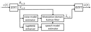
A block diagram of the modulation-domain Kalman filter based enhancement structure is shown in Fig. 1. The noisy speech, , is transformed into the STFT domain and enhancement is performed independently in each frequency bin, . The “noise model estimator” block uses the noisy speech amplitudes, , where is the index for time frame, to estimate the prior noise model. The “speech model estimator” block uses the output from a logMMSE enhancer [2, 30] to estimate the speech model. The use of a logMMSE enhancer to pre-clean the speech reduces the effect of the noise on the estimation of the speech model [21]. The modulation-domain Kalman filter combines the speech and noise models with the observed noisy speech, , to obtain an MMSE estimate of the speech spectral amplitudes, . The estimated speech is then combined with the noisy phase spectrum, , and the inverse STFT (ISTFT) is applied to obtain the enhanced speech signal, .
II-A Kalman Filter Prediction Step
The “modulation domain Kalman filter” block in Fig. 1 comprises a prediction step and an update step. For frequency bin of frame , we assume that
| (1) |
where , and are random variables representing the complex STFT coefficients of the noisy speech, clean speech and noise respectively with realizations , and . Since each frequency bin is processed independently within our algorithm, the frequency index, , will be omitted in the remainder of this paper. The random variables representing the corresponding spectral amplitudes are denoted: , , and with realizations , , and . Throughout this paper, tilde, , and breve, , diacritics will denote quantities relating to the estimated speech and noise signals respectively. The prediction model assumed for the clean speech spectral amplitude is given by
| (12) |
where denotes the state vector of speech amplitudes. denotes the transition matrix for the speech amplitudes. is a -dimensional vector. The speech transition matrix has the form
| (13) |
where is the LPC coefficient vector, is an identity matrix of size and denotes an all-zero column vector of length . represents the prediction residual signal and it has variance . The quantities , , and are defined similarly for the order- noise model. By concatenating the speech and noise state vectors, we can rewrite (12) more compactly as
| (14) |
where the quantities, , , and , have been defined in (12) and , , and . The Kalman filter prediction step estimates the state vector mean , and covariance, , at time from their estimates, and at time . The notation represents the prior estimate at acoustic frame given the observation of all the previous frames . The prediction model equations can be written as
| (15) | ||||
| (16) |
where is the covariance matrix of the prediction residual signal of speech and noise. The values of and are determined from linear predictive (LPC) analysis on modulation frames as described in Sec IV. The prior mean and covariance matrix are given by
| (18) | ||||
| (21) |
where the matrix has been defined in (14). and denote the prior estimate of the speech and noise spectral amplitude in the current frame . corresponds to the first element of the state vector and corresponds to the th elements of the state vector, . and denote the variance of the prior estimate of the speech and noise and denotes the covariance between them.
II-B Kalman Filter Update Step
For the update step, we first define a permutation matrix, , such that swaps elements and of the prior state vector so that the first two elements now correspond to the speech and noise amplitudes of frame . The covariance matrix can then be decomposed as
| (22) |
where is a matrix and is a matrix. We now define a transformed state vector, to be
where the transformation matrix is given by
where is the identity matrix.
The covariance matrix of is given by
It can be seen that the first two elements in the transformed state vector are uncorrelated with other elements. Suppose the posterior estimate of the speech and noise amplitude and the corresponding covariance matrix in the current frame are determined to be and , respectively. The state vector can be updated as
from which, applying the inverse transformation,
| (23) |
The covariance matrix, , can similarly be calculated as
| (26) | ||||
| (27) |
III Posterior distribution
III-A MMSE estimate
To perform the Kalman filter update step in Sec. II-B, we need to obtain the posterior estimate of the state vector, , and covariance matrix, . The MMSE estimate of the state vector is given by the expectation of the posterior distribution
| (28) |
where represents the observed noisy speech amplitudes up to time . The covariance matrix is given by
| (29) |
Using Bayes rule, the posterior distribution of speech amplitudes, , is calculated as
| (30) |
where is the realization of the random variable which represents the phase of the clean speech. is the observation likelihood and equals the conditional distribution of the noise, . The distribution is the prior model of the speech amplitudes and its mean and variances can be obtained from the Kalman filter prediction step given in (18) and (21). Analogous to (30), the posterior distribution of the noise, , can be calculated in a similar way.
III-B Generalized Gamma Speech Prior
In this section, which is based on [29], the distribution of the prior speech amplitude is modeled using a 2-parameter Gamma distribution
| (31) |
where is the Gamma function. The update equations induced by this prior were first derived in [29]; they are included here as (39) and (40). The two parameters, and are chosen to match the mean and variance of the predicted amplitude given by (18) and (21):
| (32) | ||||
| (33) |
Eliminating between these equations gives
| (34) |
where is the gamma function. Following [29], the solution to this equation can be approximated as where is a quartic polynomial. The observation noise is assumed to be complex Gaussian distributed with variance leading to the observation model likelihood
| (35) |
Given the assumed prior model and the observation model, the posterior distribution of the speech amplitude in (30) is given by substituting (31) and (35) into (30)
| (36) |
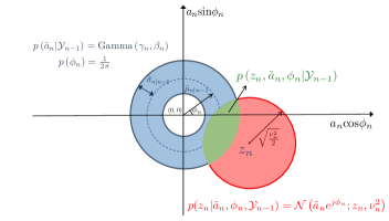
To illustrate (30), the update model is depicted in Fig. 2. The blue ring-shaped distribution centered on the origin represents the prior model, , where denotes the Gamma distribution from (31). The red circle centered on the observation, , represents the observation model . As in (30), the product of the two models gives
| (37) |
where the second term, represented by the red circle in Fig. 2, is the distribution of but offset by the observation . The green lens-shaped region of overlap represents the product of these distributions, . The posterior distribution is calculated by marginalising over the phase, , in and normalising by the integral of the green region. Substituting (36) into (28), a closed-form expression can be derived for the estimator (28) using [32, Eq. 6.643.2, 9.210.1, 9.220.2]
III-C Enhancement with Gaussring priors
In this section, we jointly model the temporal dynamics of spectral amplitudes of both the speech and noise. In this case, the observation model assumed in [34], , can be viewed as a constraint applied to the speech and noise when deriving the MMSE estimate for their amplitudes. As in Sec. II, we assume that the speech and noise are additive in the complex STFT domain. The STFT coefficients of speech and noise are assumed to have uniform prior phase distributions. To derive the Kalman filter update, the joint posterior distribution of the speech and noise amplitudes need to be estimated to apply in (23) and (27). However, in this case the normalisation term in (30) is now calculated as
| (41) |
where represents the noise amplitudes up to time and is the realization of the random variable which represents the phase of the noise. This marginalisation is mathematically intractable if the generalized Gamma distribution from (31) is assumed for both the speech and noise prior amplitude distributions.
In order to overcome this problem, in this section we assume the complex STFT coefficients to follow a “Gaussring” distribution that comprises a mixture of Gaussians whose centres lie in a circle on the complex plane.
III-C1 Gaussring distribution
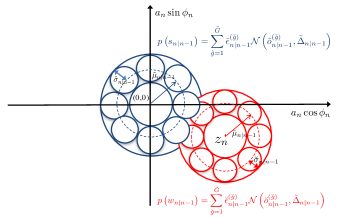
From the colored noise modulation-domain Kalman filter described in [21], the prior estimate of the amplitude of both speech and noise can be obtained. The idea of the Gaussring model is, to use a mixture of -dimensional circular Gaussians to approximate the prior distribution of the complex STFT coefficients of both the speech, , and the noise, .
For the speech coefficients, the Gaussring model is defined as
| (42) |
where is the number of Gaussian components and is the weight of the th Gaussian component. denotes the complex mean of the th Gaussian component and denotes real-valued variance (which is common to all components). The noise Gaussring model is similarly defined with parameters , and .
In this paper, we assume that the phase distribution is uniform and hence that all mixtures have equal weights of . We note however, that the Gaussring model can be extended to incorporate a prior phase distribution by using unequal weights for the mixtures. In order to fit the ring distribution to the moments of the amplitude prior from (18) and (21), and , the number of Gaussian components, , is chosen so that the mixture centres are separated by around a circle of radius in the complex plane. Accordingly, is set to be
| (43) |
where is the ceiling function.
(a)
(b)
(c)
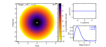
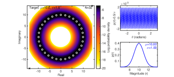
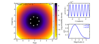
Examples of Gaussring models matching a prior estimate are shown in Fig. 3. The left plot of Fig. 3(a) shows the Gaussring distribution in the complex plane for the case for which . The white circles indicate the means of the individual Gaussian components. The two plots on the right of the figure show the marginal distributions of phase (upper plot) and magnitude (lower plot). The phase distribution is uniform to within and the magnitude distribution is almost symmetric with the correct target mean and standard deviation (printed above the plotted distribution). Fig. 3(b) shows the same plots for the case for which . In this case the phase distribution is again close to uniform while the amplitude distribution has almost the correct target mean and standard deviation but is now noticeably asymmetric. For a Rician distribution, the mean and standard deviation satisfy
| (44) |
and when , it becomes a Rayleigh distribution. Fig. 3(c) illustrates the case when the target violates this condition. In this case, the model defaults to a Rayleigh distribution whose mean square amplitude, matches that of the target.
A diagram, analogous to Fig. 3, illustrating a Gaussring model used for both the speech and noise priors in (30) is illustrated in Fig. 4. As in Fig. 4, the speech distribution is centered on the origin while the negated noise distribution is centered at the observation .
Supposing that there are components for the speech and Gaussian components for the noise, a total of Gaussian components will be obtained for the posterior distribution after combining the speech and noise prior models. The weighted product of component of speech and component of noise, is , is with parameters [35]
| (45) | ||||
| (46) | ||||
| (47) |
where denotes the value of the Gaussian distribution evaluated at . The optimal estimate of the amplitude of speech and noise is calculated as the mean of the amplitude of posterior Gaussian components as in (28).
III-C2 Moment Matching
In this subsection, we will describe how the parameters of the Gaussring model are estimated by matching the moments of the prior estimate. Because each mixture component in the Gaussring model is circular Gaussian, its amplitude is Rician distributed [33]; with a -parameter distribution given by
| (48) |
where is a modified Bessel function of the first kind and represents the realization of the speech amplitude, , or noise amplitude, . The parameters of the Rician distribution are determined by matching the mean and variance to and from (18), (21). The mean and variance of the Rician distribution in (48) are given by
| (49) | ||||
| (50) |
where and are the parameters of the Rician distribution in (48). It is difficult to invert (49) to determine and from and , so instead we use the Nakagami-m distribution to approximate the Rician distribution. There are two advantages to using this approximation. First, the parameters of the distribution can be estimated efficiently by matching the moments of the prior estimate and second, the covariance of the amplitudes of the speech and noise can be approximated efficiently. In [36], the Nakagami-m distribution is similarly used to approximate the Rician distribution in order to simplify the MMSE estimator in [1] and MAP estimator in [8].
The Nakagami-m distribution is a -parameter distribution given by [37]
The mean and variance of the Nakagami-m distribution are given by
| (51) | ||||
| (52) |
where and are the parameters of the distribution which satisfy [37]
| (53) | ||||
| (54) |
The Nakagami-m distribution is a good approximation to the Rician distribution when the parameter, , in the Nakagami-m distribution satisfies [38, 36, 39]. The parameters of the Rician distribution can be obtained from the parameters of the corresponding Nakagami-m distribution for by moment matching [39] to obtain
| (55) | ||||
| (56) |
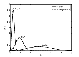
In Fig. 5, the Rician distribution and Nakamai-m distribution are compared for and , and the parameters of Rician distribution, and are calculated from and using (55) and (56). It can be seen that, the Nakagami-m distribution is a close approximation of the Rician distribution for this range of parameters.
It is still not straightforward to invert (51), (52) to determine from . However, by observing that is tightly bounded by [36]
| (57) |
we can replace this quantity by its lower bound to obtain
from which
| (58) | ||||
| (59) |
The and parameters of the corresponding Rician distribution can then be calculated from and using (55) and (56). From and the mean and covariance of each mixture of the Gaussring model can be obtained as
| (60) | ||||
| (61) | ||||
| (62) |
When the inequality in (44) is not satisfied, we use a single Gaussian component to model the distribution in (42). In this case, the prior distribution of the amplitude, , becomes a Rayleigh distribution which is a -parameter distribution. Rather than matching the mean or variance of this Rayleigh distribution to the corresponding prior, we estimate the parameter of the Rayleigh distribution by matching , which is calculated in (58) as . Thus, the mean and variance of this Gaussian distribution is given by and . The plot in Fig. 3(c) shows the Gaussring model with a target . We can see that the actual fitted mean and standard deviation deviate from the actual values and are . In this case, the model will be fitted with a mean and standard deviation which satisfy equality in (44) and give the correct value of .
III-C3 Posterior estimate
In order to determine the mean, , and covariance, , of the posterior amplitude distribution in (28), (29), we first calculate the corresponding quantities for each Gaussian component of the product, from (45), (46). We use the Nakagami-m distribution to model the amplitude distribution of this complex Gaussian, . The Nakagami-m parameters, and , are calculated in (53) and (54) from the mean and variance of the squared amplitude, denoted here by and respectively.
We define a 2-element complex Gaussian vector in which the two elements are fully correlated with each other and differ only in their means. The mean and the covariance matrix of this vector is given by
| (63) | ||||
| (64) |
in which ∘2 and denote element-wise squaring and absolute value of matrix elements. These quantities may be decomposed as
| (65) |
and
| (66) |
The parameters of the speech amplitude distribution of each component, , are obtained using (53) and (54) as
| (67) | ||||
| (68) |
The parameters of the noise amplitude distribution, , can be estimated from and in the same manner. As a result, the mean of the amplitudes of speech and noise, and , can be calculated using (51). Also, the variance of the speech and noise amplitudes, and , can be calculated using (52).
The remaining task is the calculation of the covariance for the speech and noise amplitude of each Gaussian component, . For two Nakagami-m variables with different parameters , there is no analytical solution for calculating the correlation coefficient, . However, can be well-approximated by the correlation coefficient between the squared Nakagami-m variables [41], which is given by in (66). Thus, we can obtain that and the covariance matrix, , is thereby given by .
Finally, given the mean and covariance of each Gaussian component, the posterior estimate of the speech and noise amplitudes required in (23) is given by
| (69) |
and the covariance matrix in required in (27) is given by
| (70) |
In this section, the entire process of calculating the posterior estimate of both speech and noise from their prior estimate. has been described. First, the parameters of the Nakagami-m distribution are calculated by fitting to the prior estimate of speech and noise using (58) and (59) and get the parameters of the corresponding Rician distribution from them using (55) and (56). Thus, the mean and covariance of each Gaussian component are obtained from (60) to (62) and the posterior distribution of the Gaussring components is obtained as the pairwise product of the components of speech and noise. Second, the parameters of the amplitude distribution for each component of the posterior distribution are calculated using (67) and (68). Given these parameters, the mean vector and the covariance matrix of the speech and noise amplitudes, namely and , can be calculated for each Gaussian component. Finally, the overall mean vector, , and the covariance matrix, , of the posterior estimate are obtained using (69) and (70), respectively.
IV Implementation and evaluation
In this section, the proposed modulation-domain Kalman filter based MMSE estimator using the update in Sec. III-B is denoted as MDKM and that using the Gaussring-based update in Sec. III-C is denoted as MDKR. The performance of the MDKM and MDKR enhancers are compared with that of a baseline logMMSE enhancer [2, 30], of a deep neural network (DNN) based enhancer [42] and of the colored-noise version of the modulation Kalman filter (MDKFC) enhancer from [21]. The evaluation metrics comprise segSNR [43], PESQ [44], the short-time objective intelligibility (STOI) measure [45] and the phone error rate (PER) from an automatic speech recognition (ASR) system. For the DNN based enhancer, a DNN was trained to estimate the ideal ratio mask (IRM) [42] and it had three 1024-dimensional hidden layers with rectified linear units (ReLU) [46]. Sigmoid activation functions were applied in the output layer since the targets are in the range . The average mean square error (MSE) between the predicted and true IRM was used as the cost function. We used an adaptive gradient descent algorithm [47] with a momentum of 0.5. For training the DNN, 2000 utterances were randomly selected from TIMIT training set as in [42] and they were corrupted by babble, factory, car and destroyer engine noise from the RSG-10 database [48] at , , , , and dB global SNR. The input features set was same as that in [42], which included amplitude modulation spectrogram, relative spectral transformed perceptual linear prediction coefficients (RASTA-PLP), mel-frequency cepstral coefficients (MFCC) and 64-channel Gammatone filterbank power spectra.
| Parameter | Settings |
|---|---|
| Sampling frequency |
Speech/Noise Acoustic frame length & ms Speech/Noise Acoustic frame increment ms Speech modulation frame length ms Speech modulation frame increment ms Noise modulation frame length ms Noise modulation frame increment ms Analysis-synthesis window Hamming window Speech LPC model order noise LPC model order
The evaluations used the core test set from the TIMIT database [49] as the test set, which contains 16 male and 8 female speakers each reading 8 sentences for a total of 192 sentences all with distinct texts. In order to optimize the parameters of the algorithms other than the LPC orders, a development set was used that comprised of 200 speech sentences randomly selected from the development set of the TIMIT database. A summary of the parameter settings is given in Table IV. The speech was corrupted by F16 noise from the RSG-10 database [48] and street noise from the ITU-T test signals database [50]. The sampling rate of the speech signals was 16 kHZ and noise signals were downsampled to 16 kHz. The speech LPC coefficients for the MDKM, MDKR and MDKFC algorithms were estimated from each modulation frame of the logMMSE-enhanced speech. In order to estimate the noise LPC models for the MDKR and MDKFC algorithms, we followed the procedure described in [21] in which the estimated modulation magnitude spectrum of the noise was recursively averaged during intervals that were classified as noise-only. The noise LPC coefficients were then found from the autocorrelation coefficients of the modulation magnitude spectrum of the noise. The prediction residual signal of speech and noise, which were denoted as and in in (16), were calculated as the power of the prediction errors for each modulation frame. To investigate the effect of the order on the speech modulation-domain LPC model, we calculated the prediction gain for a range of LPC orders. The prediction gain, , is defined as
| (71) |
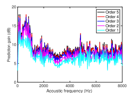
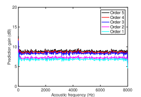
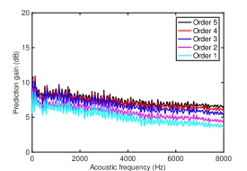
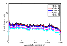
where represents the estimated speech amplitude. The expectation in (71) was taken over all acoustic frames for each frequency bin. In Fig. 6, we show the prediction gain of clean speech which was formed using speech sentences from the development set. From Fig. 6, it can be seen that, when the order, , of the modulation-domain LPC model is , the prediction gain exceeds 10 dB at most acoustic frequencies. For the acoustic frequencies accounting for most of the speech power ( Hz), the prediction gain exceeds dB. In the evaluation experiments, a modulation-domain LPC model of order 3 was used when a speech LPC model was required. Similarly, Fig. 7 shows the prediction gain of the noise LPC model for different orders, , for white noise, car noise and street noise. The plots show that the LPC models with of order 3 are able to model the noises in the modulation domain. The prediction gains of white noise are about dB over acoustic frequencies, which are fairly stable because of the stationary power distribution of white noise (the sudden drop of prediction gain at very low and very high frequencies results from the framing and windowing in the time domain). It worth noting that the predictability of the spectral amplitudes of the white noise results from the amplitude correlation that is introduced by the overlapped windows in the STFT. For car noise, because nearly all of acoustic spectral power is at low acoustic frequencies, the temporal acoustic sequences within these frequency bins are easier to predict from the previous acoustic frames, therefore the prediction gains are clearly higher at low frequencies than those at high frequencies, which are about dB. For the street noise, the gains are similar to those of the white noise and car noise. At low frequencies (10 to 200 Hz) the prediction gains are higher (about dB) than those of higher frequencies. In the experiments, a modulation-domain LPC model of order was used when a noise LPC model was required.
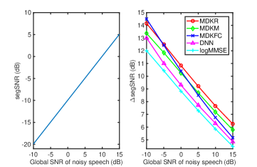
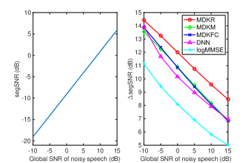
The speech signals were corrupted with additive F16 noise from the RSG-10 database [48] and street noise [50] at ,, , , and dB global SNR. All the measured values shown are averages over all the sentences in the TIMIT core test set. Figures 8 and 9 show the average segSNR of the noisy speech and the average segSNR improvement given by each algorithm over the noisy speech at each SNR for F16 noise and street noise, respectively. It can be seen that, for F16 noise, the MDKFC algorithm performs better than the MDKR, MDKM and DNN enhancers at -10 dB SNRs while at high SNRs, the MDKFR enhancer outperforms MDKFC by about 1 dB and MDKM algorithms by about 0.5 dB. At -10 dB, the DNN enhancer performs similarly to the MDKM enhancer and at other SNRs it performs worse than the MDKM enhancer by about 1 dB. For street noise, the MDKFR enhancer gives an improvement of by 2 to 3 dB over the MDKM and MDKFC enhancers over the entire range of SNRs. The DNN enhancer performs slight worse than the MDKM and MDKFC enhancers and it gives about 2.5 dB improvement over the logMMSE enhancer.
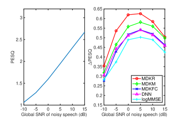
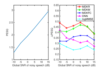
Figures 10 and 11 give the corresponding average PESQ of the noisy speech and the average PESQ performance improvement over noisy speech at each SNR. It shows that for F16 noise, at -10 dB and 15 dB SNRs, the MDKR, MDKM give similar performance and at other SNRs, the MDKR enhancer gives an improvement of about 0.1 over the MDKM and about 0.2 over the logMMSE enhancer. The MDKFC enhancer performs slightly worse that the MDKM enhancer and outperforms the logMMSE enhancer by about 0.05. The DNN enhancer gives a similar performance as the MDKFC enhancer. For street noise, the MDKR enhancer gives an improvement of around 0.1 over the MDKM enhancer at -10 dB SNR and at high SNRs (10 dB), they give similar performance. The DNN enhancer gives similar performance as the MDKM enhancer at -10 dB. At high SNRs, the performance of the DNN enhancer is worse than the MDKM and MDKFC enhancer by around 0.15 and 0.05, respectively.
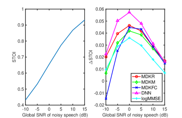
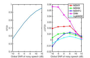
In order to assess the performance of the enhancers for speech intelligibility, the STOI measure [45] was used. Figures 12 and 13 give the average STOI of the noisy speech and the average STOI performance improvement over noisy speech at each SNR. It can be seen that for F16 noise, the DNN enhancer performs better than the other enhancers for SNRs in the range dB. At 0 dB SNR, the DNN enhancer gives an improvement of around 0.015 over the MDKR enhancer; this corresponds to an SNR gain of 0.5 dB. The MDKR enhancer gives a similar performance to the MDKM and MDKFC enhancers at high SNRs and it gives an improvement of about 0.01 over the logMMSE enhancer. For street noise, the DNN enhancer outperforms other enhancers at SNRs 10 dB and at -10 dB SNR, it gives an improvement of about 0.035 over the MDKR enhancer which corresponds to an SNR gain of 2 dB. For SNRs 5 dB, the MDKR enhancer outperforms the MDKM, MDKFC and logMMSE enhancers and at -10 dB SNR, it gives an improvement of about 0.018 over the MDKM and about 0.026 over the MDKFC and logMMSE enhancers.
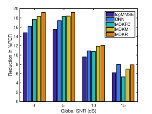
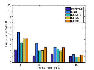
In addition to metrics for speech quality and intelligibility, we have compared the performance of the enhancers on a ASR system trained on the clean speech signals from the TIMIT dataset. The TMIT core test set was corrupted by F16 and street noise at 0, 5, 10, 15 dB SNRs. A speaker adapted DNN-hidden Markov model (HMM) hybrid system was trained using the Kaldi toolkit [51]. The input features were 40-dimensional feature-space maximum likelihood linear regression (fMLLR) transformed Mel-frequency cepstral coefficients (MFCCs). The input context window spanned from 5 frames into the past to 5 frames into the future. The DNN had 6 hidden layers and around 2000 triphone states were used as the training targets. Initialisation was performed using restricted Boltzmann machine (RBM) pre-training. The pre-trained model was then fine-tuned using the frame-level cross-entropy criterion. Sequence discriminative training using the state-level minimum Bayes risk (sMBR) criterion [52] was then applied. Figures 14 and 15 give the phone error rate (PER) improvement over noisy speech at each SNR. It shows that for F16 noise, the MDKR enhancer outperforms other enhancers at 0, 5 and 10 dB SNRs. At 0 dB SNR, the MDKR gives an improvement of 1% over the MDKM algorithm and 3% over the DNN enhancer. At 15 dB SNR, the MDKR enhancer performs similarly to the DNN enhancer and it outperforms the MDKM enhancer by 1% and the logMMSE enhancer by 1.7%. For street noise, the DNN enhancer performs slightly better than the MDKR enhancer at 0 and 5 dB SNRs and it gives an improvement of 2% over the MDKR and MDKM enhancer. However, at 10 and 15 dB, the MDKR enhancer gives similar as the DNN enhancer and they outperform other enhancers by 0.5% at 15 dB SNR.
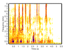
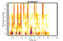
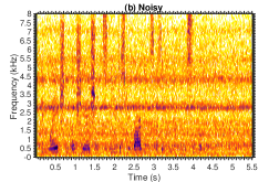
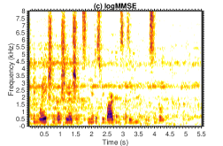
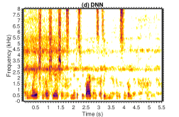
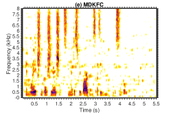
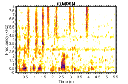
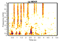
The spectrograms of speech that has been enhanced by different enhancers are shown in Fig. 16. It can be seen that the MDKR enhancer is better at suppressing noise than other enhancers, especially in the regions where speech is absent. On the other hand, the residual noise level of the DNN enhanced speech is higher than the modulation-domain Kalman filter based enhancers. Compared to the MDKM and MDKFC enhancers, the MDKR enhancer results in fewer musical noise artefacts.
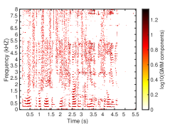
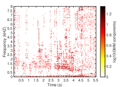
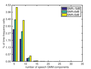
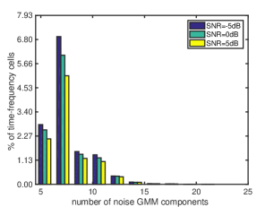
It is interesting to investigate the relationship, for each time-frequency cell, between the number of Gaussian components chosen by the proposed Gaussring model and the SNR. In Fig. 17, the number of Gaussian components for speech and noise are shown when the same utterance from Fig. 16(a) is corrupted by street noise at 10 dB SNR. For better visualisation, the numbers of the Gaussian components have been transformed into log10 domain. We can see that for time-frequency cells where the speech power is high, the predicted speech amplitudes have a high confidence and thereby the ratio of the prior mean and standard deviation is large. Thus, the speech Gaussring model has a large number of Gaussian components. Conversely, for time-frequency cells where the noise power is high, the noise Gaussring model has a large number of Gaussian components. In Fig. 18, the histograms show the distributions of the number of Gaussian components of speech and noise respectively for speech that is corrupted by street noise at , and dB SNRs. When plotting the histograms, for clarity the histogram plots omit the bars corresponding to (i.e. a single GMM component); these correspond to cells in which the ratio and the Gaussring model backs off to a Rayleigh distribution. It can be seen that, as the SNR increases, the number of speech components in each histogram cell increases while the number of noise components decreases.
V Conclusion
In this paper, a model-based estimator for the spectral amplitudes of clean speech based on a modulation-domain Kalman filter has been proposed. The novelty of this proposed enhancer over our previous work is that it can incorporate the temporal dynamics of both the speech and noise spectral amplitudes. To obtain the optimal estimate, a Gaussring model was proposed in which mixtures of Gaussians were employed to model the prior distribution of the speech and noise in the complex Fourier domain, leading to the proposed MDKR enhancer. Over a wide range of SNRs, the MDKR enhancer resulted in enhanced speech with higher scores for objective speech quality measures than competing algorithms. For speech intelligibility, the MDKR enhancer gave worse but yet comparable performance when compared to the DNN enhancer. The ASR experiments showed that the MDKR enhancer performed better than competing algorithms for F16 noise and for street noise, the MDKR enhancer performed similarly to the DNN enhancer for SNRs dB.
References
- [1] Y. Ephraim and D. Malah. Speech enhancement using a minimum-mean square error short-time spectral amplitude estimator. IEEE Trans. Acoust., Speech, Signal Process., 32(6):1109–1121, December 1984.
- [2] Y. Ephraim and D. Malah. Speech enhancement using a minimum mean-square error log-spectral amplitude estimator. IEEE Trans. Acoust., Speech, Signal Process., 33(2):443–445, April 1985.
- [3] R. Martin. Speech enhancement based on minimum mean-square error estimation and supergaussian priors. IEEE Trans. Speech Audio Process., 13(5):845–856, September 2005.
- [4] T. Lotter and P. Vary. Speech enhancement by MAP spectral amplitude estimation using a super-gaussian speech model. EURASIP Journal on Applied Signal Processing, 2005(7):1110–1126, January 2005.
- [5] P. C. Loizou. Speech enhancement based on perceptually motivated Bayesian estimators of the magnitude spectrum. IEEE Trans. Speech Audio Process., 13(5):857–869, August 2005.
- [6] J. S. Erkelens, R. C. Hendriks, R. Heusdens, and J. Jensen. Minimum mean-square error estimation of discrete fourier coefficients with generalized gamma priors. IEEE Trans. Speech Audio Process., 15(6):1741–1752, August 2007.
- [7] J. Porter S. and Boll. Optimal estimators for spectral restoration of noisy speech. In Proc. IEEE Intl. Conf. on Acoustics, Speech and Signal Processing (ICASSP), volume 9, pages 53–56, March 1984.
- [8] P. J. Wolfe and S. J. Godsill. Efficient alternatives to the Ephraim and Malah suppression rule for audio signal enhancement. EURASIP Journal on Applied Signal Processing, 2003(10):1043–1051, September 2003.
- [9] P. J. Wolfe and S. J. Godsill. Towards a perceptually optimal spectral amplitude estimator for audio signal enhancement. In Proc. IEEE Intl. Conf. on Acoustics, Speech and Signal Processing (ICASSP), volume 2, pages II:821–II:824 vol.2, June 2000.
- [10] P. J. Wolfe and S. J. Godsill. Simple alternatives to the Ephraim and Malah suppression rule for speech enhancement. In Proc. IEEE Signal Processing Workshop on Statistical Signal Processing, pages 496–499, August 2001.
- [11] C. H. You, S. N. Koh, and S. Rahardja. -order MMSE spectral amplitude estimation for speech enhancement. IEEE Trans. Speech Audio Process., 13(4):475–486, June 2005.
- [12] E. Plourde and B. Champagne. Auditory-based spectral amplitude estimators for speech enhancement. IEEE Trans. Speech Audio Process., 16(8):1614–1623, Nov 2008.
- [13] R. Drullman, J. M. Festen, and R. Plomp. Effect of reducing slow temporal modulations on speech reception. J. Acoust. Soc. Am., 95(5):2670–2680, May 1994.
- [14] R. Drullman, J. M. Festen, and R. Plomp. Effect of temporal envelope smearing on speech reception. J. Acoust. Soc. Am., 95(2):1053–1064, February 1994.
- [15] L. Atlas and S. A. Shamma. Joint acoustic and modulation frequency. EURASIP Journal on Applied Signal Processing, 2003(7):668–675, June 2003.
- [16] M. Elhilali, T. Chi, and S. A. Shamma. A spectro-temporal modulation index (STMI) for assessment of speech intelligibility. Speech Communication, 41(2-3):331–348, 2003.
- [17] F. Dubbelboer and T. Houtgast. The concept of signal-to-noise ratio in the modulation domain and speech intelligibility. J. Acoust. Soc. Am., 124(6):3937–3946, December 2008.
- [18] H. Hermansky, E. A. Wan, and C. Avendano. Speech enhancement based on temporal processing. In Proc. IEEE Intl. Conf. on Acoustics, Speech and Signal Processing (ICASSP), volume 1, pages 405 –408, May 1995.
- [19] T. H. Falk, S. Stadler, W. B. Kleijn, and W. Y. Chan. Noise suppression based on extending a speech-dominated modulation band. In Proc. Interspeech Conf., pages 970–973, August 2007.
- [20] K. Paliwal, K. Wojcicki, and B. Schwerin. Single-channel speech enhancement using spectral subtraction in the short-time modulation domain. Speech Communication, 52(5):450–475, 2010.
- [21] S. So and K. Paliwal. Modulation-domain Kalman filtering for single-channel speech enhancement. Speech Communication, 53(6):818–829, July 2011.
- [22] K. Paliwal, B. Schwerin, and K. Wójcicki. Speech enhancement using a minimum mean-square error short-time spectral modulation magnitude estimator. Speech Communication, 54(2):282–305, February 2012.
- [23] Y. Wang and M. Brookes. Speech enhancement using a robust Kalman filter post-processing in the modulation domain. In Proc. IEEE Intl. Conf. on Acoustics, Speech and Signal Processing (ICASSP), pages 7457–7461, May 2013.
- [24] Y. Wang and M. Brookes. A subspace method for speech enhancement in the modulation domain. In Proc. European Signal Processing Conf. (EUSIPCO), 2013.
- [25] Y. Wang. Speech enhancement in the modulation domain. PhD thesis, Imperial College London, 2015.
- [26] S. Boll. Suppression of acoustic noise in speech using spectral subtraction. IEEE Trans. Acoust., Speech, Signal Process., 27(2):113 – 120, April 1979.
- [27] A. Rix, J. Beerends, M. Hollier, and A. Hekstra. Perceptual evaluation of speech quality (PESQ) - a new method for speech quality assessment of telephone networks and codecs. In Proc. IEEE Intl. Conf. on Acoustics, Speech and Signal Processing (ICASSP), pages 749–752, May 2001.
- [28] K. Paliwal and A. Basu. A speech enhancement method based on Kalman filtering. In Proc. IEEE Intl. Conf. on Acoustics, Speech and Signal Processing (ICASSP), pages 177 – 180, April 1987.
- [29] Y. Wang and M. Brookes. Speech enhancement using an MMSE spectral amplitude estimator based on a modulation domain Kalman filter with a Gamma prior. In Proc. IEEE Intl. Conf. on Acoustics, Speech and Signal Processing (ICASSP), pages 5225–5229, March 2016.
- [30] M. Brookes. VOICEBOX: A speech processing toolbox for MATLAB. http://www.ee.imperial.ac.uk/hp/staff/dmb/voicebox/voicebox.html, 1998-2016.
- [31] J. D. Gibson, B. Koo, and S. D. Gray. Filtering of colored noise for speech enhancement and coding. IEEE Trans. Signal Process., 39(8):1732–1742, August 1991.
- [32] A. Jeffrey and D. Zwillinger. Table of Integrals, Series, and Products. Academic Press, 6th edition, 2000.
- [33] F. Olver, D. Lozier, R. F. Boiszert, and C. W. Clark, editors. NIST Handbook of Mathematical Functions: Companion to the Digital Library of Mathematical Functions. Cambridge University Press, 2010. URL: http://dlmf.nist.gov/13.
- [34] S. So, K.K. Wójcicki, and K.K. Paliwal. Single-channel speech enhancement using Kalman filtering in the modulation domain. In Eleventh Annual Conference of the International Speech Communication Association, 2010.
- [35] M. Brookes. The matrix reference manual. http://www.ee.imperial.ac.uk/hp/staff/dmb/matrix/intro.html, 1998-2015.
- [36] D. Xie and W. Zhang. Estimating speech spectral amplitude based on the Nakagami approximation. IEEE Signal Processing Letters, 21(11):1375–1379, Nov 2014.
- [37] J. Cheng and N. C. Beaulieu. Maximum-likelihood based estimation of the Nakagami-m parameter. IEEE Communications letters, 5(3):101–103, 2001.
- [38] L. C. Wang and C. T. Lea. Co-channel interference analysis of shadowed Rician channels. IEEE Communications Letters, 2(3):67–69, March 1998.
- [39] P. J. Crepeau. Uncoded and coded performance of MFSK and DPSK in Nakagami fading channels. IEEE Transactions on Communications, 40(3):487–493, March 1992.
- [40] K. S. Miller. Complex stochastic processes: an introduction to theory and application. Addison-Wesley Publishing Company, Advanced Book Program, 1974.
- [41] Z. Song, K. Zhang, L. Guan, and Y. Liang. Generating correlated Nakagami fading signals with arbitrary correlation and fading parameters. In Proc. Intl. Conf. Commun. (ICC), volume 3, pages 1363–1367 vol.3, April 2002.
- [42] Y. Wang, A. Narayanan, and D. Wang. On training targets for supervised speech separation. IEEE/ACM Trans. on Audio, Speech and Language Processing, 22(12):1849–1858, 2014.
- [43] Y. Hu and P. C. Loizou. Evaluation of objective measures for speech enhancement. In Proc. Interspeech Conf., pages 1447–1450, 2006.
- [44] A. W. Rix, J. G. Beerends, D.-S. Kim, P. Kroon, and O. Ghitza. Objective assessment of speech and audio quality - technology and applications. IEEE Trans. Audio, Speech, Lang. Process., 14(6):1890–1901, November 2006.
- [45] C. H. Taal, R. C. Hendriks, R. Heusdens, and J. Jensen. An algorithm for intelligibility prediction of time frequency weighted noisy speech. IEEE Trans. Audio, Speech, Lang. Process., 19(7):2125–2136, September 2011.
- [46] M. D. Zeiler, M. Ranzato, R. Monga, M. Mao, K. Yang, Q. V. Le, P. Nguyen, A. Senior, V. Vanhoucke, J. Dean, et al. On rectified linear units for speech processing. In Proc. IEEE Intl. Conf. on Acoustics, Speech and Signal Processing (ICASSP), pages 3517–3521. IEEE, 2013.
- [47] J. Duchi, E. Hazan, and Y. Singer. Adaptive subgradient methods for online learning and stochastic optimization. Journal of Machine Learning Research, 12(Jul):2121–2159, 2011.
- [48] H. J. M. Steeneken and F. W. M. Geurtsen. Description of the RSG.10 noise data-base. Technical Report IZF 1988–3, TNO Institute for perception, 1988.
- [49] J. S. Garofolo. Getting started with the DARPA TIMIT CD-ROM: An acoustic phonetic continuous speech database. Technical report, National Institute of Standards and Technology (NIST), Gaithersburg, Maryland, December 1988.
- [50] ITU-T P.501. Test signals for use in telephonometry, August 1996.
- [51] D. Povey, A. Ghoshal, G. Boulianne, L. Burget, O. Glembek, N. Goel, M. Hannemann, P. Motlicek, Y. Qian, P. Schwarz, et al. The kaldi speech recognition toolkit. In Proc. IEEE workshop on automatic speech recognition and understanding, 2011.
- [52] K. Veselỳ, A. Ghoshal, L. Burget, and D. Povey. Sequence-discriminative training of deep neural networks. In Proc. Interspeech Conf., pages 2345–2349, 2013.
![[Uncaptioned image]](/html/1707.02651/assets/photo_wang.jpg) |
Yu Wang (S’12-M’15) received the Bachelor’s degree from Huazhong University of Science and Technology, Wuhan, China, in 2009, the M.Sc. degree in communications and signal processing and the Ph.D. degree in signal processing, both from Imperial College, London, U.K. in 2010 and 2015, respectively. Since August 2015 he has been working as a Research Associate at the Machine Intelligence Laboratory in the Engineering Department, University of Cambridge. His current research interests include robust speech recognition, speech and audio signal processing and automatic spoken language assessment. |
![[Uncaptioned image]](/html/1707.02651/assets/photo_brookes.jpg) |
Mike Brookes Mike Brookes (M’88) is a Reader (Associate Professor) in Signal Processing in the Department of Electrical and Electronic Engineering at Imperial College London. After graduating in Mathematics from Cambridge University in 1972, he worked at the Massachusetts Institute of Technology and, briefly, the University of Hawaii before returning to the UK and joining Imperial College in 1977. Within the area of speech processing, he has concentrated on the modelling and analysis of speech signals, the extraction of features for speech and speaker recognition and on the enhancement of poor quality speech signals. He is the primary author of the VOICEBOX speech processing toolbox for MATLAB. Between 2007 and 2012 he was the Director of the Home Office sponsored Centre for Law Enforcement Audio Research (CLEAR) which investigated techniques for processing heavily corrupted speech signals. He is currently principal investigator of the E-LOBES project that seeks to develop environment-aware enhancement algorithms for binaural hearing aids. |