Rapidity dependence of proton cumulants and correlation functions

Abstract

The dependence of multi-proton correlation functions and cumulants on the acceptance in rapidity and transverse momentum is studied. We find that the preliminary data of various cumulant ratios are consistent, within errors, with rapidity and transverse momentum independent correlation functions. However, rapidity correlations which moderately increase with rapidity separation between protons are slightly favored. We propose to further explore the rapidity dependence of multi-particle correlation functions by measuring the dependence of the integrated reduced correlation functions as a function of the size of the rapidity window.

I Introduction

One of the central goals in strong interaction research is to explore the phase diagram of QCD. Of particular interest is the search for a possible first-order phase coexistence region and its associated critical point. A significant effort in this search, experimentally as well as theoretically, is concentrating on the measurements and calculations of correlations and cumulants of conserved charges. A particular emphasis has been put on the cumulants of the baryon number Stephanov et al. (1998); Stephanov (2009); Skokov et al. (2011); Friman et al. (2011); Adamczyk et al. (2014a, b), see also Borsanyi et al. (2012); Bazavov et al. (2012); Bellwied et al. (2015); Gavai and Gupta (2011); Kitazawa et al. (2014); Asakawa and Kitazawa (2016); Mukherjee et al. (2016); Herold et al. (2016); Chatterjee et al. (2016); Lacey et al. (2016); Hippert and Fraga (2017); Rougemont et al. (2017); Almasi et al. (2017); He and Luo (2017) (see, e.g., Koch (2010) for an overview). Interpreting these higher order cumulants and their measurements, however, is not a straightforward exercise as discussed, e.g., in Bzdak et al. (2013); Skokov et al. (2013); Bzdak and Koch (2012, 2015); Luo (2015a); Nonaka et al. (2016); Westfall (2015); Fecková et al. (2015); Bzdak et al. (2016); Braun-Munzinger et al. (2017); Bluhm et al. (2017); Xu (2017); Nonaka et al. (2017); Garg and Mishra (2017). Also, different, although related, ideas, based on an intermittency analysis in the transverse momentum phase space have been explored Anticic et al. (2010, 2015); Antoniou et al. (2016).

Recently, it has been pointed out Ling and Stephanov (2016); Bzdak et al. (2017a), (see also Kitazawa and Luo (2017); He and Luo (2017)), that it may be more instructive to study (integrated) multi-particle correlations instead of cumulants. In the limit when anti-particles can be ignored, which is the case for anti-protons at low beam energies, the integrated multi-particle correlations are linear combinations of the various cumulants and thus can be extracted easily from the measured cumulants. This has been done on the basis of preliminary data on proton cumulants from the STAR collaboration Luo (2015b). It was found that the systems created at low beam energies ($7.7-11.5{\rm\,GeV}$) exhibit sizable three- and strong four-proton correlations Bzdak et al. (2017a); Luo and Xu (2017). Indeed, as pointed out in Bzdak et al. (2017b), in order to reproduce the observed magnitude of these correlations one has, for example, to assume a strong presence of eight-nucleon (or four-proton) clusters in the system. In addition to the sheer magnitude of the correlations, the centrality and rapidity dependence of these correlations give additional insight into properties of the systems created in these collisions Bzdak et al. (2017a).

In this paper we will explore the rapidity and to some extent transverse momentum dependence of multi-particle correlations in more detail. One of our motivations is a recent preliminary observation by the STAR collaboration Jowzaee ; Lipiec regarding the rapidity dependence of the two-proton correlation function. Within the rapidity window $|y|<0.8$, STAR finds that across all RHIC energies the two proton reduced correlation function (see the definition in section II) in central Au+Au collisions is strongly increasing with the rapidity separation, $y_{1}-y_{2}$, between the two protons. The shape of the correlation function can be approximately described by

$$c_{2}(y_{1}-y_{2})=c_{2}^{0}+\gamma_{2}\left(y_{1}-y_{2}\right)^{2},\qquad\gamma_{2}>0,$$ (1)

where $c_{2}^{0}$ is the value at $y_{1}-y_{2}=0$, and $\gamma_{2}$ is a positive number, with $\gamma_{2}\sim 2\times 10^{-2}$ at $\sqrt{s}=7.7{\rm\,GeV}$ Jowzaee . Taking such a correlation at face value, one would conclude that protons prefer to be separated in rapidity, or, in other words, they seem to repel each other. The shape of the correlation function is roughly energy independent, which is rather surprising since protons at, say, $7.7$ GeV, originate almost exclusively from the target and projectile nuclei whereas at $200{\rm\,GeV}$, the protons at mid-rapidity mostly are produced.

The apparent anti-correlation between two protons was first observed in $e^{+}e^{-}$collisions at $\sqrt{s}=29$ GeV Aihara et al. (1986). Recently an analogous observation was made by the ALICE collaboration in the context of the two-baryon azimuthal correlations Adam et al. (2016). This measurement also found similar anti-correlations between protons and lambdas, suggesting that the observed effects are not due to the Pauli exclusion principle or electromagnetic interactions. To our knowledge, the origin of this effect remains an open question, which is important to resolve. Formation of clusters, as suggested in Bzdak et al. (2017b), and as expected close to a critical point and a phase transition, would naively lead to attractive correlations in rapidity (i.e., protons would prefer to have similar rapidity) and not anti-correlations. However, we should keep in mind that these correlations are in rapidity and not in configuration space. Also, one should note that this effect, which, so far, is only observed for two-particle correlations, may not be inconsistent with the negative value for the integrated two-particle correlations extracted from the cumulant measurements Bzdak et al. (2017a); Luo and Xu (2017). In general, the sign of an integrated multi-particle correlation also is driven by a pedestal. For example, in the case of two protons, $c_{2}^{0}$ in Eq. (1) may depend on the fluctuations of the volume, or rather the number of wounded nucleons Bialas et al. (1976); Skokov et al. (2013); Bzdak et al. (2017b); Braun-Munzinger et al. (2017), and is not necessarily related to a possible repulsion or attraction in rapidity between protons.

Clearly the rapidity dependence of the proton correlations need to be studied to gain further insight into the aforementioned sizable three-proton and strong four-proton correlations observed at low energies. It is the purpose of this paper to start exploring this issue. To this end we study the dependence of the multi-proton correlation functions on rapidity, and, to some extent, on the transverse momentum. We show that the preliminary STAR data Luo (2015b) are consistent with constant multi-proton correlation functions and slightly favor multi-proton anti-correlations in rapidity. We also demonstrate that these correlations can be constrained further by measuring integrated reduced or normalized correlation functions as a function of the rapidity window $\Delta y$.

This paper is organized as follows. In the next section we introduce the notation and discuss the behavior of cumulants and correlation functions in the limits of small and large acceptances. Next we analyze the preliminary STAR data and extract some trends about the rapidity dependence of three-proton and four-proton correlations. We also will propose a means to extract more detailed information about the multi-particle correlations. In the last section we conclude with a discussion of the essential results.

II Notation and comments

In this paper we focus on protons only and in the following we denote the proton number by $N$ and its deviation from the mean by $\delta N=N-\left\langle N\right\rangle$. Here $\left\langle N\right\rangle$ is the mean number of protons at a given centrality. The cumulants of the proton distribution function as measured by the STAR collaboration are then given by

$$K_{1}\equiv\langle N\rangle;\quad K_{2}\equiv\langle(\delta N)^{2}\rangle;\quad K_{3}\equiv\langle\left(\delta N\right)^{3}\rangle;\quad K_{4}\equiv\langle\left(\delta N\right)^{4}\rangle-3\langle(\delta N)^{2}\rangle^{2}.$$ (2)

As already eluded to in the Introduction, the cumulants can be expressed in terms of the multi-particle integrated correlation functions Bzdak et al. (2017a), which also are known as factorial cumulants Ling and Stephanov (2016)

$$K_{2} = \left\langle N\right\rangle+C_{2},$$ (3)

$$K_{3} = \left\langle N\right\rangle+3C_{2}+C_{3},$$ (4)

$$K_{4} = \left\langle N\right\rangle+7C_{2}+6C_{3}+C_{4},$$ (5)

where

$$C_{2} = \int dy_{1}dy_{2}C_{2}(y_{1},y_{2})$$ (6)

$$= \int dy_{1}dy_{2}\left[\rho_{2}(y_{1},y_{2})-\rho(y_{1})\rho(y_{2})\right],$$

and similar for higher order correlation functions. See, e.g., Ref. Bzdak and Bozek (2016) for explicit definitions of the correlation functions up to the sixth order. In Eq. (6) $C_{2}(y_{1},y_{2})$ is the two-particle rapidity correlation function, $\rho_{2}(y_{1},y_{2})$ is the two-particle rapidity density, and $\rho(y)$ is the single-particle rapidity distribution. The generalization of Eqs. (3-5) to two species of particles can be found in the Appendix of Ref. Bzdak et al. (2017a). Here and in the following $y_{i}$ denotes rapidity or in general, a set of variables under consideration $(y_{i},p_{t,i},\varphi_{i})$.

It is a convenient and common practice to define the reduced correlation function

$$c_{n}\left(y_{1},...,y_{n}\right)=\frac{C_{n}\left(y_{1},...,y_{n}\right)}{\rho\left(y_{1}\right)\cdots\rho\left(y_{n}\right)}.$$ (7)

The integral of the reduced correlation function over some given acceptance range, we subsequently will call, for the lack of a better term, “coupling”

$$c_{n}=\frac{C_{n}}{\left\langle N\right\rangle^{n}}=\frac{\int\rho\left(y_{1}\right)\cdots\rho\left(y_{n}\right)c_{n}\left(y_{1},...,y_{n}\right)dy_{1}\cdots dy_{n}}{\int\rho\left(y_{1}\right)\cdots\rho\left(y_{n}\right)dy_{1}\cdots dy_{n}}.$$ (8)

The cumulants $K_{n}$ then may be expressed in terms of the couplings $c_{n}$,

$$K_{2} = \left\langle N\right\rangle+\left\langle N\right\rangle^{2}c_{2},$$ (9)

$$K_{3} = \left\langle N\right\rangle+3\left\langle N\right\rangle^{2}c_{2}+\left\langle N\right\rangle^{3}c_{3},$$ (10)

$$K_{4} = \left\langle N\right\rangle+7\left\langle N\right\rangle^{2}c_{2}+6\left\langle N\right\rangle^{3}c_{3}+\left\langle N\right\rangle^{4}c_{4}.$$ (11)

Of course, mathematically, the cumulants $K_{1}=\langle N\rangle$, $K_{2}$, $K_{3}$, and $K_{4}$ carry exactly the same information as [$C_{2}$, $C_{3}$, $C_{4}$] or [$c_{2}$, $c_{3}$, $c_{4}$]. However, as already discussed in Bzdak et al. (2017a), studying cumulants may not be the best way to extract information about the dynamics of the system, since: (i) cumulants mix the correlation functions of different orders and (ii) they might be dominated by a trivial term $\langle N\rangle$ even in the presence of interesting dynamics.

One such example, where the trivial term $\langle N\rangle$ dominates and thus hides the interesting physics is the limit of small acceptance as we will discuss next.

II.1 Effective Poisson limit

Before we discuss the rapidity and transverse momentum dependence of the various cumulants and correlations, let us briefly remind ourselves what happens if one considers the limit of small or vanishing acceptance. Here, we will restrict ourselves to correlations in rapidity, however our arguments will be general and apply to any variables. Suppose that particles are measured in a rapidity interval $y_{0}\leq y\leq y_{0}+\Delta y$ and that $\Delta y\rightarrow 0$. Let us first consider two-particle correlations. For sufficiently small $\Delta y$ any reasonable correlation function $c_{2}(y_{1},y_{2})$ may be approximated by a constant. As a consequence, for sufficiently small $\Delta y$, the coupling, $c_{2}$, is independent of $\Delta y$, as can be seen from Eq. (8). In other words, suppose that $c_{2}(y_{1},y_{2})\simeq c_{2}^{0}$ for very small $\Delta y$, then

$$c_{2}=\frac{\int_{\Delta y}\rho(y_{1})\rho(y_{2})c_{2}(y_{1},y_{2})dy_{1}dy_{2}}{\int_{\Delta y}\rho(y_{1})\rho(y_{2})dy_{1}dy_{2}}\simeq c_{2}^{0}.$$ (12)

We emphasize that $c_{2}^{0}$ may assume any value. However, whatever the value of $c_{2}^{0}$, in the limit of $\Delta y\rightarrow 0$, we have $\left\langle N\right\rangle\rightarrow 0$ and $K_{2}\simeq\left\langle N\right\rangle$ (see Eq. (9)). Exactly the same argument holds for any $K_{n}$, and we obtain $K_{n}\simeq\left\langle N\right\rangle$ and consequently all cumulant ratios equal to unity, $K_{n}/K_{m}\simeq 1$.

Therefore, even in the presence of sizable correlations, their effects on the cumulants are suppressed for small acceptance. Actually, as can be seen from Eqs. (9)-(11), it is the number of particles which determines if the cumulants are dominated by $\langle N\rangle$ and, thus, their ratios are close to unity. For example, if $\langle N\rangle^{4}c_{4}<<\langle N\rangle$, the fourth order cumulant, $K_{4}$, is practically not sensitive to four-proton correlations even if $c_{4}$ is different from zero and may carry some interesting information. Therefore, even for large acceptance the cumulants are close to the Poisson limit if one is dealing with rare particles. This may very well be the reason that for low energies STAR observes a cumulant ratio of $K_{4}/K_{2}\simeq 1$ for anti-protons, and it would be interesting to measure the couplings, $c_{n}$, for anti-protons in order to see if anti-protons exhibit the same correlations as protons at low energies.

Clearly measuring cumulants and looking for the deviation from the Poisson limit is not the most optimal way to extract possible non-trivial correlations resulting from criticality etc. Instead, one either should directly measure the differential multi-particle correlation (Eq. (7)) or, at the very least, extract the couplings, $c_{n}$, Eq. (8). Their dependence on the acceptance does reflect a change in physics and is not simply a consequence of a change in the number of particles.

After having investigated the case of small acceptance let us next turn to the opposite limit of (nearly) full acceptance.

II.2 Full acceptance

Let us next study what happens in the situation when all baryons, including the spectators, are detected. In this case (again, we consider low energies and neglect anti-baryons) $N=\langle N\rangle=B$, where $B$ is the total baryon number of the entire system. Therefore, $\delta N=0$ and obviously $K_{n}=0$ for $n\geq 2$. Using Eqs. (3-5) and (9-11) we obtain

$$C_{2}=-B,\qquad C_{3}=2B,\qquad C_{4}=-6B,$$ (13)

and

$$c_{2}=-\frac{1}{B},\qquad c_{3}=\frac{2}{B^{2}},\qquad c_{4}=-\frac{6}{B^{3}}.$$ (14)

We note that this is a general result and it is insensitive to the presence of any dynamics other than global baryon number conservation.

Finally let us note that $K_{3}/K_{2}\rightarrow-1$ and $K_{4}/K_{2}\rightarrow 1$ when we approach the limit of full acceptance. To see this let us consider a region in phase space, denoted by $(a)$, and the remaining phase space, or complement, which we denote by $(b)$. Since the baryon number is conserved, having $N_{(a)}$ baryons in region $(a)$ implies $N_{(b)}=B-N_{(a)}$ baryons in the complement, $(b)$. Since $\delta B=0$ we have

$$\delta N_{(b)}=\delta(B-N_{(a)})=-\delta N_{(a)},$$ (15)

and consequently

$$K_{n,(a)} = K_{n,(b)}\quad n=2,4,6,...,$$

$$K_{n,(a)} = -K_{n,(b)}\quad n=3,5,7,....$$ (16)

Here $K_{n,(a)}$ is the cumulant measured in region $(a)$ and $K_{n,(b)}$ is the cumulant in a remaining part of the full phase space, $(b)$. This is a rather nontrivial and general consequence of baryon conservation. A more rigorous derivation is presented in the Appendix.

In the previous subsection we argued that for very small acceptance the cumulant ratio goes to $1$ and thus the cumulant ratio for the full acceptance goes to $-1$ for $K_{3}/K_{2}$ and to $1$ for $K_{4}/K_{2}$. The integrated correlation functions and the couplings, on the other hand, do not show such a symmetry between a given region of phase space and its compliment. This is shown in detail in the Appendix but can already be inferred from the fact that in the limit of full acceptance the couplings are determined entirely by the total baryon number $B$. In the limit of vanishing acceptance, however, other physics also affects the value of the couplings, as discussed in Section II.1.

Having discussed the limits of small and full acceptances we now turn to the rapidity dependence of the cumulants and correlation functions.

III Results

In this section we discuss in detail the rapidity and, to some extent, the transverse momentum dependence of multi-proton cumulants and correlation functions. First, we will explore the limit of rapidity and transverse momentum independent correlations. Next we will discuss to which extent the present preliminary STAR data allow us to set limits on the rapidity dependence of the underlying correlations.

III.1 Constant correlation

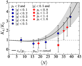
Figure 1: The cumulant ratio $K_{4}/K_{2}$ in central $0-5\%$ Au+Au collisions at $\sqrt{s}=7.7$ GeV as a function of the number of measured protons, $\left\langle N\right\rangle$, for different acceptance windows in rapidity and transverse momentum (in units of GeV). For all data points $p_{t}>0.4{\rm\,GeV}$. The black solid line represents a prediction based on a constant correlation function, see Eq. (17). The shaded band is driven mostly by the large experimental uncertainty of $K_{4}$. Based on preliminary STAR data Luo (2015b).

Let us start with the simplest assumption namely that the reduced correlation function does not depend on rapidity and transverse momentum, i.e.,

$$c_{n}(y_{1},p_{t1},...,y_{n},p_{tn})=const=c_{n}^{0}.$$ (17)

This rather extreme assumption, however, is, as we will show below, consistent with the preliminary STAR data at $7.7$ GeV (see also Bzdak et al. (2017a)). In addition, in this case the couplings $c_{n}$ do not depend on rapidity and transverse momentum either, as can be seen from Eq. (8)

$$c_{n}=c_{n}^{0}.$$ (18)

The multi-particle integrated correlation functions, $C_{n}=\langle N\rangle^{n}c_{n}$, and cumulants, $K_{n}$, in turn depend on the acceptance only through their dependence on the number of protons $\left\langle N\right\rangle$, see Eqs. (9-11). Therefore, in Fig. 1 we plot $K_{4}/K_{2}$ as measured by STAR as a function of $\left\langle N\right\rangle$ for different rapidity and transverse momentum intervals.

The black solid line in Fig. 1 represents a prediction based on a constant correlation function. In this calculation we have three unknown parameters, $c_{2}^{0},$ $c_{3}^{0}$ and $c_{4}^{0}$. Since these numbers do not depend on acceptance we determine them from the preliminary data for $|y|<0.5$ ($\Delta y=1$) and $0.4<p_{t}<2$ GeV, that is, from the maximal acceptance currently available. Here we use Eqs. (9-11) and the values for $\langle N\rangle$, $K_{2}$, $K_{3}$ and $K_{4}$ shown in Ref. Luo (2015b). To determine $\left\langle N\right\rangle$ at a given acceptance region we assume the single proton rapidity distribution to be flat as a function of rapidity, i.e., $\left\langle N\right\rangle=\left\langle N_{\Delta y=1}\right\rangle\Delta y$ and for the transverse momentum single proton distribution we take $\rho(p_{t})\sim p_{t}\exp(-m_{t}/T)$ with $T=0.27$ GeV and $m_{t}=(m^{2}+p_{t}^{2})^{1/2}$ with $m=0.94$ GeV. Both these assumptions are well supported by experimental data Adamczyk et al. (2017); Anticic et al. (2011). Having $c_{n}^{0}$, we can predict the cumulants or the correlation functions for any acceptance characterized by $\left\langle N\right\rangle$, whether in transverse momentum or in rapidity.

Interestingly we find that, except for one point at $|y|<0.5$ and $0.4<p_{t}<1.2$ GeV, all the points follow, within the admittedly large experimental error bars, one universal curve consistent with a constant correlation function. The fact that the rapidity dependence of the cumulant ratio $K_{4}/K_{2}$ is consistent with long-range rapidity correlations already has been found in Bzdak et al. (2017a). That the transverse momentum dependence is also consistent with long-range correlations is new. If correct, it would, for example, imply that the cumulant ratio $K_{4}/K_{2}$ has roughly the same value (close to unity) for a transverse momentum range of $0.8{\rm\,GeV}<p_{t}<2{\rm\,GeV}$ as the value for the range of $0.4{\rm\,GeV}<p_{t}<0.8{\rm\,GeV}$ since, in both $p_{t}$ windows, $\langle N\rangle$ is approximately the same. The result for the $p_{t}$-range of $0.4{\rm\,GeV}<p_{t}<0.8{\rm\,GeV}$ has been published by the STAR collaboration in Adamczyk et al. (2014a).

Of course, the error bars in the preliminary STAR data are rather sizable and, therefore, a mild dependence of the correlation function on rapidity (and transverse momentum) cannot be ruled out. In addition, as already mentioned in the Introduction, the preliminary, explicit measurement of the two-proton correlation function Jowzaee ; Lipiec does exhibit an increase with increasing rapidity difference of a proton pair, $y_{1}-y_{2}$. To explore this further we next will allow for some mild rapidity dependence of the correlation function.

III.2 Rapidity dependent correlation

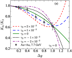
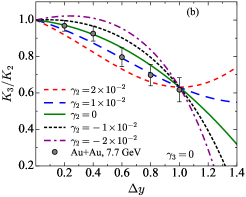
Figure 2: The cumulant ratio $K_{3}/K_{2}$ in central Au+Au collisions at $\sqrt{s}=7.7$ GeV as a function of the rapidity acceptance $\Delta y$, $|y|<\Delta y/2$, for (a) $\gamma_{2}=0$ and different values of $\gamma_{3}$ from Eq. (19) and (b) $\gamma_{3}=0$ and different values of $\gamma_{2}$. Based on preliminary STAR data Luo (2015b).

In the previous subsection we demonstrated that the STAR data for $K_{4}/K_{2}$ at $7.7$ GeV are consistent with a constant multi-proton correlation function. Here we study how sensitive the cumulant ratios and correlations are to a certain (weak) rapidity dependence. To this end we consider the leading correction to a constant correlation function, which should be even in $y_{i}-y_{k}$. Thus we explore the following ansätze for the reduced correlation functions

$$c_{2}(y_{1},y_{2}) = c_{2}^{0}+\gamma_{2}\left(y_{1}-y_{2}\right)^{2},$$

$$c_{3}(y_{1},y_{2},y_{3}) = c_{3}^{0}+\gamma_{3}\tfrac{1}{3}\left[\left(y_{1}-y_{2}\right)^{2}+\left(y_{1}-y_{3}\right)^{2}+\left(y_{2}-y_{3}\right)^{2}\right],$$

$$c_{4}(y_{1},y_{2},y_{3},y_{4}) = c_{4}^{0}+\gamma_{4}\tfrac{1}{6}\left[\left(y_{1}-y_{2}\right)^{2}+\left(y_{1}-y_{3}\right)^{2}+\left(y_{1}-y_{4}\right)^{2}\right.$$ (19)

$$\,\,\,\,\,\,\,\,\,\,\,\,\,\,\,\,\,\,\,\,\,\,\,\,\,\left.+\left(y_{2}-y_{3}\right)^{2}+\left(y_{2}-y_{4}\right)^{2}+\left(y_{3}-y_{4}\right)^{2}\right],$$

where $\gamma_{n}$ measures the deviation from $c_{n}(y_{1},...,y_{n})=const$. Note that we have constructed the correlation function such that positive values of $\gamma_{n}$ result in growing correlations with rapidity separation between particles. We further note that the above form for the two-proton reduced correlation function, $c_{2}(y_{1},y_{2})$, is supported by the preliminary STAR data Jowzaee ; Lipiec where $\gamma_{2}>0$, that is, two protons do not want to occupy the same rapidity. Our simple formulas for $c_{3}$ and $c_{4}$ are not supported by any known data, however, we believe they should serve as a reasonable representation for the correlation if the distance in rapidity between protons is not too large. Within the region of validity of our simple ansatz, the coefficients $\gamma_{n}$ have a clear physical interpretation, and here we will constrain their values or at least their signs. To this end we will use the preliminary STAR data for $K_{3}/K_{2}$ and $K_{4}/K_{2}$. Although, as already pointed out, the rapidity dependence of these cumulant ratios is consistent with constant correlations, we will see that the data allow for excluding certain values for $\gamma_{n}$ and possibly even determine their sign.

Taking the above relations and integrating in Eq. (8) over $|y_{i}|<\Delta y/2$ we obtain for the couplings

$$c_{n}(\Delta y)=\frac{C_{n}}{\left\langle N\right\rangle^{n}}=c_{n}^{0}+\gamma_{n}\frac{1}{6}(\Delta y)^{2}.$$ (20)

The couplings, $c_{n}(\Delta y)$, which depend on the region of acceptance, $\Delta y$ ($|y_{i}|<\Delta y/2$), should not be confused with the reduced correlation functions, $c_{n}(y_{1},...,y_{n})$, which depend on the rapidities of the individual particles. As before, for a given $\gamma_{n}$ the constant term, $c_{n}^{0}$ is extracted from the STAR data at $\Delta y=1$ ($|y|<0.5$) and $0.4<p_{t}<2$ GeV. Consequently, $c_{n}^{0}$ will depend on the choice of $\gamma_{n}$.

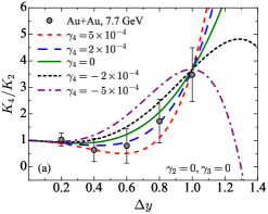
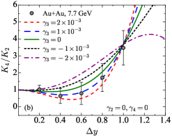
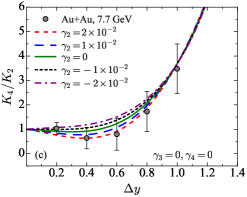
Figure 3: The cumulant ratio $K_{4}/K_{2}$ in central Au+Au collisions at $\sqrt{s}=7.7$ GeV as a function of the rapidity acceptance $\Delta y$, $|y|<\Delta y/2$, for (a) different values of $\gamma_{4}$, (b) $\gamma_{3}$ and (c) $\gamma_{2}$ from Eq. (19). Based on preliminary STAR data Luo (2015b).

In Fig. 2 we show $K_{3}/K_{2}$ for different values of $\gamma_{3}$ in panel (a) and $\gamma_{2}$ in panel (b). We observe that, as already discussed before, the preliminary STAR data are consistent with a constant correlation function in rapidity ($\gamma_{2}=\gamma_{3}=0$). However, a small positive value of $\gamma_{2}\sim 10^{-2}$ or $\gamma_{3}\sim 10^{-3}$ would actually improve the agreement slightly. The negative values for $\gamma_{2}$ and $\gamma_{3}$, on the other hand, appear to be disfavored so are large positive values. The same is true for the comparison with the $K_{4}/K_{2}$ cumulant ratio, which we show in Fig. 3. Again, the data are consistent with constant rapidity correlation functions or perhaps slightly positive values for $\gamma_{2}$, $\gamma_{3}$, or $\gamma_{4}$, whereas negative values for $\gamma_{n}$ seem to be disfavored.

Also, the overall picture of slightly “repulsive” corrections to the constant correlation functions, i.e., $\gamma_{n}\geq 0$ is consistent with the preliminary STAR data on the two-proton rapidity correlation function, which, as discussed in the Introduction, indicates a peculiar repulsion between protons in rapidity. As these new STAR measurements only address two proton correlations, the most direct test would be a comparison of the rapidity dependence of the second order cumulant or integrated correlation. This is shown in Fig. 4. Unfortunately, at present there are no data available for rapidity intervals other than $\Delta y=1$, and since this point is used for the determination of the overall constant, $c_{2}^{0}$, no constraint can be made at this time. However, we wish to emphasize the strong dependence compared to the size of the error bar. Indeed, the increase in the correlation exhibited in the preliminary STAR data for the differential correlation functions Jowzaee ; Lipiec is consistent with $\gamma_{2}\sim 2\times 10^{-2}$, which would correspond to the red dashed curve in Fig. 4. Given the size of the error bar at $\Delta y=1$, it should be possible to discriminate from a constant correlation function, shown by the green solid line. Needless to say, such a measurement of the rapidity dependence of $K_{2}/K_{1}$ would be very valuable to ensure the consistency of the cumulant measurement with that of the differential correlation function.

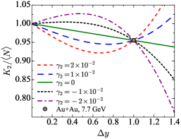
Figure 4: The cumulant ratio $K_{2}/K_{1}$ in central Au+Au collisions at $\sqrt{s}=7.7$ GeV as a function of the rapidity acceptance $\Delta y$, $|y|<\Delta y/2$, for different values of $\gamma_{2}$. Based on preliminary STAR data Luo (2015b).

Of course it would be even more valuable to have information about the differential three- and four-particle correlation functions. Therefore, we propose, as a first step, to measure the rapidity dependence of the couplings, $c_{n}(\Delta y)$. This will allow for a direct determination of the coefficients, $\gamma_{n}$, as we demonstrate in Fig. 5, where we plot $c_{n}(\Delta y)/c_{n}^{0}-1$ for $\gamma_{2}=10^{-2}$, $\gamma_{3}=10^{-3}$ and $\gamma_{4}=2\times 10^{-4}$. We note that $c_{n}(\Delta y)$ is rather sensitive to $\gamma_{n}$.

In principle it would also be interesting to measure $c_{n}(\Delta y)$ for higher $n$ such as $n=5$ and $6$. In this case

$$c_{5}(y_{1},...,y_{5}) = c_{5}^{0}+\gamma_{5}\tfrac{1}{10}\sum\nolimits_{i,k=1;\text{ }i<k}^{5}\left(y_{i}-y_{k}\right)^{2},$$

$$c_{6}(y_{1},...,y_{6}) = c_{6}^{0}+\gamma_{6}\tfrac{1}{15}\sum\nolimits_{i,k=1;\text{ }i<k}^{6}\left(y_{i}-y_{k}\right)^{2},$$ (21)

and $c_{n}(\Delta y)$ is given by Eq. (20).

IV Discussion and conclusions

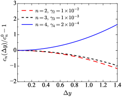
Figure 5: The ratio of the couplings $c_{n}(\Delta y)/c_{n}^{0}-1$, see Eqs. (8,20) for $\gamma_{2}=10^{-2}$, $\gamma_{3}=10^{-3}$ and $\gamma_{4}=2\times 10^{-4}$. $\Delta y$ denotes the size of the rapidity window, $|y|<\Delta y/2$, which the reduced correlation functions are integrated over.

Before we conclude let us discuss the main findings of this paper.

• The preliminary data for the proton cumulant ratio $K_{4}/K_{2}$ obtained by the STAR collaboration at $\sqrt{s}=7.7$ GeV are consistent with long-range correlations in both rapidity and transverse momentum. As a result the cumulants effectively depend only on the number of protons $\left\langle N\right\rangle$ in the acceptance. Therefore, we predict that new measurements with increased acceptance will lead to even larger values for the $K_{4}/K_{2}$. Naturally this increase will be limited eventually by global charge conservation as discussed in Bzdak et al. (2013), and the ansatz for the correlation function, Eq. (17) will have its limitation for large $\Delta y$. Consequently our present prediction for large $\Delta y>1$ needs to be taken with a grain of salt.

• Allowing for small deviation from a constant value we find that a slightly “repulsive” rapidity dependence is favored by the data. By “repulsive” we mean that the correlation function increases with increasing rapidity separation between protons. Or in other words, we find that $\gamma_{n}>0$ in Eq. (19) is favored. Perhaps this may be the first evidence for “repulsive” three-proton and four-proton correlations.

• Clearly, as demonstrated in Fig. 5, a measurement of the couplings as a function of the rapidity and transverse momentum windows would be very valuable to shed more light on the ranges and detailed shapes of the correlation functions.

• Finally we want to reiterate that the fact that cumulant ratios for small acceptance or, more precisely for a small number of particles, are close to unity does not necessarily imply the absence of correlations. This is demonstrated in Fig. 1 where we actually assume a constant correlation. In addition, this may also be the reason that anti-protons show a cumulant ratio of $K_{4}/K_{2}\simeq 1$ at low energies whereas the protons show a significant deviation from unity.
  We further demonstrated that global baryon conservation fully determines the cumulant ratios, integrated correlation functions, and couplings close to the full acceptance regardless of any additional dynamics. In addition we showed that, as a result of baryon number conservation, the cumulants in a given phase-space window and their complements are closely related, see Eq. (16) and the Appendix.

To summarize, we have studied the rapidity dependence of cumulants, integrated correlation functions and couplings based on the presently available preliminary STAR collaboration data Luo (2015b). Although we found that, within the present experimental errors the data are consistent with rapidity independent correlations, a slightly “repulsive” component seems to be favored. This would be consistent with the preliminary measurement of two-particle differential proton correlations by STAR Jowzaee ; Lipiec . To gain further insight, in particular, into the three-proton and four-proton correlations, we proposed to measure the dependence of the couplings as a function of the rapidity window.

Appendix A Full acceptance

Suppose we divide the full phase space into the two, not necessarily equal sized regions denoted by the subscripts $(a)$ and $(b)$. Let $P_{(a)}(N_{(a)})$ be the probability to observe $N_{(a)}$ baryons in the phase space region $(a)$. The probability to have $N_{(b)}$ baryons in the remaining part of the entire phase space, $P_{(b)}(N_{(b)})$, is given by $P_{(b)}(N_{(b)})=P_{(a)}(N_{(a)})=P_{(a)}(B-N_{(b)})$ since $N_{(a)}=B-N_{(b)}$, where $B$ is the conserved number of baryons. Here we assume that we can ignore anti-baryons. The cumulant generating function for the phase space region $(a)$, $h_{(a)}(t)$ is given by

$$h_{(a)}(t) = \log\left[\sum\nolimits_{N_{(a)}}P_{(a)}(N_{(a)})e^{N_{(a)}t}\right]$$ (22)

$$= \log\left[\sum\nolimits_{N_{(b)}}P_{(a)}(B-N_{(b)})e^{(B-N_{(b)})t}\right]$$

$$= \log\left[\sum\nolimits_{N_{(b)}}P_{(b)}(N_{(b)})e^{(B-N_{(b)})t}\right]$$

$$= h_{(b)}(-t)+Bt,$$

where $h_{(b)}(t)$ is the cumulant generating function for phase space region $(b)$. The cumulants in the two regions, $(a)$ and $(b)$, are given by the derivatives at $t=0$,

$$K_{n,(a)}=\frac{d^{n}}{dt^{n}}h_{(a)}(t)|_{t=0},\quad K_{n,(b)}=\frac{d^{n}}{dt^{n}}h_{(b)}(t)|_{t=0}.$$ (23)

Thus we get for $n=1$

$$\left\langle N_{(a)}\right\rangle=K_{1,(a)}=B-K_{1,(b)}=B-\left\langle N_{(b)}\right\rangle,$$ (24)

and for $n\geq 2$

$$K_{n,(a)}=(-1)^{n}K_{n,(b)}.$$ (25)

.

Given this relation between the cumulants of the two regions and using Eqs. (2)-(5) we also can find the relation between the integrated correlation functions $C_{{n,(a)}}$ and $C_{n,(b)}$ in regions $(a)$ and $(b)$, respectively.

$$C_{2,(a)} = -B+2\langle N_{(b)}\rangle+C_{2,(b)},$$

$$C_{3,(a)} = 2B-6\langle N_{(b)}\rangle-6C_{2,(b)}-C_{3,(b)},$$

$$C_{4,(a)} = -6B+24\langle N_{(b)}\rangle+36C_{2,(b)}+12C_{3,(b)}+C_{4,(b)}.$$ (26)

Clearly, the integrated correlation functions do not show any symmetry between the two complementary regions of the phase space. The same is also true for the couplings $c_{n}$. In the limit where $\left\langle N_{(a)}\right\rangle\rightarrow B$ and thus $\left\langle N_{(b)}\right\rangle\rightarrow 0$ we find, following the above equations, that $C_{2,(a)}\rightarrow-B$, $C_{3,(a)}\rightarrow 2B$, and $C_{4,(a)}\rightarrow-6B$. In this case, the couplings become $c_{2,(a)}\rightarrow-\frac{1}{B}$, $c_{3,(a)}\rightarrow\frac{2}{B^{2}}$, and $c_{4,(a)}\rightarrow-\frac{6}{B^{3}}$, and again are determined entirely by the total baryon number $B$. For the complementary region $(b)$, on the other hand, we have the limit of $\left\langle N_{b}\right\rangle\rightarrow 0$, in which case, as discussed in Section II.1, dynamics beyond baryon number conservation also affects the couplings.

References

- Stephanov et al. (1998) M. A. Stephanov, K. Rajagopal, and E. V. Shuryak, Phys. Rev. Lett. 81, 4816 (1998), hep-ph/9806219 .
- Stephanov (2009) M. Stephanov, Phys.Rev.Lett. 102, 032301 (2009), arXiv:0809.3450 [hep-ph] .
- Skokov et al. (2011) V. Skokov, B. Friman, and K. Redlich, Phys.Rev. C83, 054904 (2011), arXiv:1008.4570 [hep-ph] .
- Friman et al. (2011) B. Friman, F. Karsch, K. Redlich, and V. Skokov, Eur.Phys.J. C71, 1694 (2011), arXiv:1103.3511 [hep-ph] .
- Adamczyk et al. (2014a) L. Adamczyk et al. (STAR), Phys. Rev. Lett. 112, 032302 (2014a), arXiv:1309.5681 [nucl-ex] .
- Adamczyk et al. (2014b) L. Adamczyk et al. (STAR), Phys. Rev. Lett. 113, 092301 (2014b), arXiv:1402.1558 [nucl-ex] .
- Borsanyi et al. (2012) S. Borsanyi, Z. Fodor, S. D. Katz, S. Krieg, C. Ratti, et al., JHEP 1201, 138 (2012), arXiv:1112.4416 [hep-lat] .
- Bazavov et al. (2012) A. Bazavov et al. (HotQCD Collaboration), Phys.Rev. D86, 034509 (2012), arXiv:1203.0784 [hep-lat] .
- Bellwied et al. (2015) R. Bellwied, S. Borsanyi, Z. Fodor, S. D. Katz, A. Pasztor, C. Ratti, and K. K. Szabo, Phys. Rev. D92, 114505 (2015), arXiv:1507.04627 [hep-lat] .
- Gavai and Gupta (2011) R. V. Gavai and S. Gupta, Phys. Lett. B696, 459 (2011), arXiv:1001.3796 [hep-lat] .
- Kitazawa et al. (2014) M. Kitazawa, M. Asakawa, and H. Ono, Phys.Lett. B728, 386 (2014), arXiv:1307.2978 [nucl-th] .
- Asakawa and Kitazawa (2016) M. Asakawa and M. Kitazawa, Prog. Part. Nucl. Phys. 90, 299 (2016), arXiv:1512.05038 [nucl-th] .
- Mukherjee et al. (2016) A. Mukherjee, J. Steinheimer, and S. Schramm, (2016), arXiv:1611.10144 [nucl-th] .
- Herold et al. (2016) C. Herold, M. Nahrgang, Y. Yan, and C. Kobdaj, Phys. Rev. C93, 021902 (2016), arXiv:1601.04839 [hep-ph] .
- Chatterjee et al. (2016) A. Chatterjee, S. Chatterjee, T. K. Nayak, and N. R. Sahoo, J. Phys. G43, 125103 (2016), arXiv:1606.09573 [nucl-ex] .
- Lacey et al. (2016) R. A. Lacey, P. Liu, N. Magdy, B. Schweid, and N. N. Ajitanand, (2016), arXiv:1606.08071 [nucl-ex] .
- Hippert and Fraga (2017) M. Hippert and E. S. Fraga, (2017), arXiv:1702.02028 [hep-ph] .
- Rougemont et al. (2017) R. Rougemont, R. Critelli, J. Noronha-Hostler, J. Noronha, and C. Ratti, (2017), arXiv:1704.05558 [hep-ph] .
- Almasi et al. (2017) G. A. Almasi, B. Friman, and K. Redlich, (2017), arXiv:1703.05947 [hep-ph] .
- He and Luo (2017) S. He and X. Luo, (2017), arXiv:1704.00423 [nucl-ex] .
- Koch (2010) V. Koch, in Relativistic Heavy Ion Physics, Landolt-Boernstein New Series I, Vol. 23, edited by R. Stock (Springer, Heidelberg, 2010) pp. 626–652, arXiv:0810.2520 [nucl-th] .
- Bzdak et al. (2013) A. Bzdak, V. Koch, and V. Skokov, Phys. Rev. C87, 014901 (2013), arXiv:1203.4529 [hep-ph] .
- Skokov et al. (2013) V. Skokov, B. Friman, and K. Redlich, Phys. Rev. C88, 034911 (2013), arXiv:1205.4756 [hep-ph] .
- Bzdak and Koch (2012) A. Bzdak and V. Koch, Phys. Rev. C86, 044904 (2012), arXiv:1206.4286 [nucl-th] .
- Bzdak and Koch (2015) A. Bzdak and V. Koch, Phys. Rev. C91, 027901 (2015), arXiv:1312.4574 [nucl-th] .
- Luo (2015a) X. Luo, Phys. Rev. C91, 034907 (2015a), arXiv:1410.3914 [physics.data-an] .
- Nonaka et al. (2016) T. Nonaka, T. Sugiura, S. Esumi, H. Masui, and X. Luo, Phys. Rev. C94, 034909 (2016), arXiv:1604.06212 [nucl-th] .
- Westfall (2015) G. D. Westfall, Phys. Rev. C92, 024902 (2015), arXiv:1412.5988 [nucl-th] .
- Fecková et al. (2015) Z. Fecková, J. Steinheimer, B. Tomášik, and M. Bleicher, Phys. Rev. C92, 064908 (2015), arXiv:1510.05519 [nucl-th] .
- Bzdak et al. (2016) A. Bzdak, R. Holzmann, and V. Koch, Phys. Rev. C94, 064907 (2016), arXiv:1603.09057 [nucl-th] .
- Braun-Munzinger et al. (2017) P. Braun-Munzinger, A. Rustamov, and J. Stachel, Nucl. Phys. A960, 114 (2017), arXiv:1612.00702 [nucl-th] .
- Bluhm et al. (2017) M. Bluhm, M. Nahrgang, S. A. Bass, and T. Schaefer, Eur. Phys. J. C77, 210 (2017), arXiv:1612.03889 [nucl-th] .
- Xu (2017) H.-J. Xu, Phys. Lett. B765, 188 (2017), arXiv:1612.06485 [nucl-th] .
- Nonaka et al. (2017) T. Nonaka, M. Kitazawa, and S. Esumi, Phys. Rev. C95, 064912 (2017), arXiv:1702.07106 .
- Garg and Mishra (2017) P. Garg and D. K. Mishra, (2017), arXiv:1705.01256 [nucl-th] .
- Anticic et al. (2010) T. Anticic et al. (NA49), Phys. Rev. C81, 064907 (2010), arXiv:0912.4198 [nucl-ex] .
- Anticic et al. (2015) T. Anticic et al. (NA49), Eur. Phys. J. C75, 587 (2015), arXiv:1208.5292 [nucl-ex] .
- Antoniou et al. (2016) N. G. Antoniou, N. Davis, and F. K. Diakonos, Phys. Rev. C93, 014908 (2016), arXiv:1510.03120 [hep-ph] .
- Ling and Stephanov (2016) B. Ling and M. A. Stephanov, Phys. Rev. C93, 034915 (2016), arXiv:1512.09125 [nucl-th] .
- Bzdak et al. (2017a) A. Bzdak, V. Koch, and N. Strodthoff, Phys. Rev. C95, 054906 (2017a), arXiv:1607.07375 [nucl-th] .
- Kitazawa and Luo (2017) M. Kitazawa and X. Luo, (2017), arXiv:1704.04909 [nucl-th] .
- Luo (2015b) X. Luo (STAR), Proceedings, 9th International Workshop on Critical Point and Onset of Deconfinement (CPOD 2014): Bielefeld, Germany, November 17-21, 2014, PoS CPOD2014, 019 (2015b), arXiv:1503.02558 [nucl-ex] .
- Luo and Xu (2017) X. Luo and N. Xu, Nucl. Sci. Tech. 28, 112 (2017), arXiv:1701.02105 [nucl-ex] .
- Bzdak et al. (2017b) A. Bzdak, V. Koch, and V. Skokov, Eur. Phys. J. C77, 288 (2017b), arXiv:1612.05128 [nucl-th] .
- (45) S. Jowzaee (STAR), Talk presented at the the XXVI international conference on ultrarelativistic heavy-ion collisions (Quark Matter 2017), Chicago, February 2017 .
- (46) A. Lipiec (STAR), Talk presented at the XII Workshop on Particle Correlations and Femtoscopy, Amsterdam, June 2017 .
- (47) W. Llope (STAR), Talk presented at the Conference on Critical Point and Onset of Deconfinement (CPOD 2017), Stony Brook, August 2017 .
- Aihara et al. (1986) H. Aihara et al. (TPC/Two Gamma), Phys. Rev. Lett. 57, 3140 (1986).
- Adam et al. (2016) J. Adam et al. (ALICE), (2016), arXiv:1612.08975 [nucl-ex] .
- Bialas et al. (1976) A. Bialas, M. Bleszynski, and W. Czyz, Nucl. Phys. B111, 461 (1976).
- Bzdak and Bozek (2016) A. Bzdak and P. Bozek, Phys. Rev. C93, 024903 (2016), arXiv:1509.02967 [hep-ph] .
- Adamczyk et al. (2017) L. Adamczyk et al. (STAR), (2017), arXiv:1701.07065 [nucl-ex] .
- Anticic et al. (2011) T. Anticic et al. (NA49), Phys. Rev. C83, 014901 (2011), arXiv:1009.1747 [nucl-ex] .