Locating large flexible ligands on proteins

Abstract

Many biologically important ligands of proteins are large, flexible, and often charged molecules that bind to extended regions on the protein surface. It is infeasible or expensive to locate such ligands on proteins with standard methods such as docking or molecular dynamics (MD) simulation. The alternative approach proposed here is the scanning of a spatial and angular grid around the protein with smaller fragments of the large ligand. Energy values for complete grids can be computed efficiently with a well-known Fast Fourier Transform accelerated algorithm and a physically meaningful interaction model. We show that the approach can readily incorporate flexibility of protein and ligand. The energy grids (EGs) resulting from the ligand fragment scans can be transformed into probability distributions, and then directly compared to probability distributions estimated from MD simulations and experimental structural data. We test the approach on a diverse set of complexes between proteins and large, flexible ligands, including a complex of Sonic Hedgehog protein and heparin, three heparin sulfate substrates or non-substrates of an epimerase, a multi-branched supramolecular ligand that stabilizes a protein-peptide complex, and a flexible zwitterionic ligand that binds to a surface basin of a Kringle domain. In all cases the EG approach gives results that are in good agreement with experimental data or MD simulations.

Bioinformatics and Computational Biophysics, Essen]Bioinformatics and Computational Biophysics, Faculty of Biology, University of Duisburg-Essen, Universitätstraße 7, 45141 Essen, Germany Institute of Organic Chemistry, Essen]Institute of Organic Chemistry, University of Duisburg-Essen, Universitätstraße 7, 45141 Essen, Germany Bioinformatics and Computational Biophysics, Essen]Bioinformatics and Computational Biophysics, Faculty of Biology, University of Duisburg-Essen, Universitätstraße 7, 45141 Essen, Germany Biomedical Engineering, Eindhoven]Laboratory of Chemical Biology, Department of Biomedical Engineering and Institute for Complex Molecular Systems, Eindhoven University of Technology, Den Dolech 2, 5612 AZ Eindhoven, The Netherlands Institute of Organic Chemistry, Essen]Institute of Organic Chemistry, University of Duisburg-Essen, Universitätstraße 7, 45141 Essen, Germany Bioinformatics and Computational Biophysics, Essen]Bioinformatics and Computational Biophysics, Faculty of Biology, University of Duisburg-Essen, Universitätstraße 7, 45141 Essen, Germany +49 (0)201 183 4391 +49 (0)201 183 3437 FFT

1 Introduction

The prediction of binding poses of small molecules with a mixture of polar and hydrophobic groups that bind with high affinity in protein pockets has been one of the dominating problems in biomolecular modeling, and the successes in this endeavor had a major impact in the life sciences and drug design. However, many biologically important interactions are almost the exact opposite to this scenario: large, flexible ligands bind to protein surfaces, their binding is often transient, and charge-charge interactions are essential. Examples are interactions between secreted proteins and the extracellular matrix of glycosaminoglycans^{1, 2}, interactions of virus proteins with host receptors in viral cell entry ³, or interactions of T-cell receptors with MHC I-peptide complexes ⁴. Another interesting case is the design of novel supramolecular ligands that bind protein surfaces with many low affinity interactions but overall high avidity ⁵. How can we model and predict complexes of proteins with such large, flexible ligands that are often charged or zwitterionic? Sometimes it is possible to predict binding modes of large, flexible ligands by docking suitable fragments with methods developed for small molecule docking ⁶. This is less promising if binding occurs not in typical small molecule binding pockets, but at the protein surface, often involving charged residues with long, flexible side chains, as for instance in the case of protein-glycosaminoglycan binding. In these cases, interactions could be characterized by Molecular Dynamics simulation (MD) or related sampling methods ⁷, though the necessary computational effort can be excessive.

A promising alternative are approaches that evaluate energies for ligand positions on a 3D-grid around the target protein. Although they have mainly been used for docking ⁸, i.e. for locating optimal ligand positions and poses, they allow in principle for a characterization of the complete target protein surface and environment with respect to ligand binding energetics. A great advantage of grid-based approaches is that the protein-ligand interaction energies on the grid can be evaluated efficiently by exploiting discrete Fast Fourier Transforms (FFT) ^{9, 10, 11, 12}. Since we are mostly interested in interactions of proteins with charged ligands, another candidate method for characterizing the interaction energetics around the target protein is the solution of the Poisson-Boltzmann equation, typically also with efficient grid-based methods ^{13, 14}.

In the work presented here we assess the suitability of fast grid-based methods for predicting binding modes of large, flexible, and usually charged ligands on protein surfaces. These ligands not only defy docking methods, but they force us also to abandon the notion of the well-defined binding pose, because their size and flexibility, and the fact that they bind to extended protein surface regions will make binding more fuzzy.

One way to account for this uncertainty while still retaining a quantitative approach is to predict affinity distributions or probability densities for the ligand, or at least for those functional groups that likely mediate binding. The abovementioned grid-based methods ^{9, 10, 11, 12} are attractive because they could provide exactly this information in an efficient way. Generally, the approach proposed here assumes that we can infer the location of a large, flexible ligand from probability distributions of characteristic fragments, and that these fragment probability distributions can be computed efficiently and sufficiently accurate by grid based, FFT accelerated scanning. We also demonstrate that flexibility of the target protein and of ligand fragments can be incorporated easily.

To test the above assumptions we have applied the method to four different test cases that cover several scenarios of practical interest: the surface binding of heparin to Sonic Hedgehog protein for which we compare several methods and experimental data, the specific interactions of an epimerase with three different heparan sulfate substrates or non-substrates as an example for specificity of interaction, the stabilization of a protein-peptide complex by an artificial multi-branched supramolecular ligand as example of a large non-polymeric ligand, and the binding of a flexible zwitterionic ligand to a Kringle domain.

2 Methods and molecules

2.1 Workflow

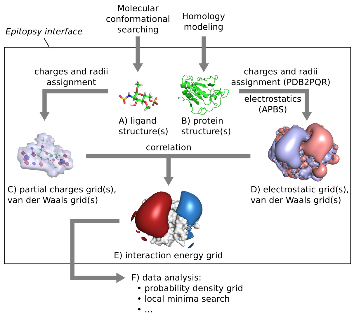
Figure 1: Workflow for the computation of (interaction) energy grids (EGs) with Epitopsy. Representative conformations of ligand fragments and target protein are required as input (A, B). Charges and radii of both interaction partners are assigned (C, D). The EG for a ligand-protein pair as “correlation” with FFTs as described in text (E). EGs can then be analyzed in various ways outside Epitopsy (F).

Figure 1 shows the overall workflow of our grid-based analysis. Each of the steps will be described in the following section. To make our results reproducible we provide our experimental Epitopsy software as free open source code at
https://github.com/BioinformaticsBiophysicsUDE/Epitopsy.

2.2 Molecular dynamics (MD) simulation

MD simulations were used, first, to determine representative ligand conformations as input of Epitopsy (Fig 1A), and second, as a reference method to estimate probability densities of ligand fragments around the target protein that can then be compared to corresponding probabilities computed from (interaction) energy grids (EGs) generated by Epitopsy.

Molecular Dynamics (MD) simulations were run with Gromacs 4.6.7¹⁵ using the Amber ff99SB force field¹⁶ for proteins and GLYCAM 06h-2¹⁷ for saccharides. Phosphorylated serine parameters were obtained from the literature¹⁸. Non-standard amino acids in ligand QQJ-096 (succinic acid, phenyl trihydrazine, N-acetyl-lysine and GCP) were parametrized for the ff99SB force field according to the procedure described in the original ff94 article¹⁹. Atomic charges were derived from electrostatic potential maps calculated at the HF/6-31** level of theory in Gaussian09 version A.02²⁰ and fitted to the residues using the Restrained Electrostatic Potential method ^{21, 22}. Force constant parameters were obtained by chemical analogy with readily available parameters in ff94²³. Topology files were created with the pdb2gmx module of Gromacs for the protein, and with the TLEaP module of Amber v12.21²⁴ with the AmberTools suite v13.22 for the ligands. Amber topologies were converted to Gromacs topologies by ACPype²⁵.

Proteins and ligands were solvated in a dodecahedron box of SPC/E water molecules²⁶ with a 10 Å minimum separation between the protein and the box boundaries. The system was neutralized by addition of Na⁺ and Cl^- ions to a final ionic strength of $0.15$ mol/l. The system was energy-minimized by steepest-descent to a total force of $1800$ $\mathrm{k}\mathrm{J}\,\mathrm{m}\mathrm{o}\mathrm{l}^{-1}\,\mathrm{n}\mathrm{m}^{-1}$, equilibrated for 5 ns in the NVT ensemble with constrained heavy atoms, and for 5 ns in the NPT ensemble without constraints. Production simulation was run in the NPT ensemble for 200 ns if not mentioned otherwise. Temperature was stabilized at 300 K in the NVT and NPT ensembles by the V-rescale thermostat²⁷, while the pressure was stabilized at 1 atm in the NPT ensemble by the Berendsen barostat (equilibration) or Parinello-Rahman barostat (data production)²⁸. Simulations were carried out on a GPU (GeForce 970 and GeForce 1070, CUDA 8) using a time step of 2 fs, the Verlet scheme²⁹ for neighbor search with a 10 Å cutoff, the Particle Mesh Ewald method³⁰ for electrostatic calculations, and the LINCS algorithm³¹ for bond restraints.

Representative structures were extracted from trajectories based on mutual RMSDs, using the g_rms tool in Gromacs to produce 2D RMSD plots, the pam (partition around medoids) tool from R package cluster, version 2.0.6, in R v3.3.1³² to find the clusters, and the cluster.stats function of R package fpc, version 2.1.10, to validate the clustering based on silhouette coefficients.

When high flexibility in the ligand prevented the extraction of representative structures, the ligand trajectory was projected on a grid to produce a probability distribution of the ligand around the protein. To this end, the simulation box was discretized and we counted for each grid point the number of MD frames where it was within the van der Waals radius of a ligand atom. The resulting count was divided either by the total number of frames in the trajectory to yield a grid point sampling frequency, or by the sum of the grid point frequencies to yield a (ligand) probability density. The latter was used to compute cumulative density plots and to draw Highest Density Regions³³ (HDR) in a molecular visualization software. When comparing electrostatic, energy and probability density grids, all the compared grids were laid out with the same resolution, dimensions and offset.

EGs, HDR and molecules were visualized with PyMOL v1.7.4.0³⁴ compiled from sources.

2.3 Protein structures

Crystal structures were refined in Modeller 9.17^{35, 36} to restore missing residues when necessary (Table Supporting information). Candidate structures were required to minimize the DOPE and molpdf score. In case of ties, the refined model with lowest RMSD to the template was selected.

2.4 Assignment of charges and radii

For the computation of EGs, charges and radii have to be assigned to the ligand (Fig 1C) and protein (Fig 1D). Charges and atomic radii were added on the proteins using PDB2PQR v2.0.0^{37, 38} at neutral pH and 298 K using the Amber force field option. Ligand charges were determined with one of the following methods, as specified in the text: with PDB2PQR (default), specialized MM forcefields, from an electrostatic potential fit using the Merz-Singh-Kollman scheme^{39, 40} in Gaussian 2009 A02²⁰ at the HF/6-31G** level of theory, or using the Gasteiger-Marsili method^{41, 42} in OpenBabel v2.3.2⁴³. Information on atomic radii was added to the ligand atoms by OpenBabel.

2.5 Electrostatics

For the target protein the electrostatic field was computed by solving the non-linear Poisson-Boltzmann equation with APBS version 1.4.1¹⁴ at 310K, with an ionic concentration of $0.15$ mol/l and relative dielectric permittivities $\varepsilon_{r}^{\text{vacuum}}=2$ and $\varepsilon_{r}^{\text{water}}=79$.

2.6 Energy grid computation

The central part of the workflow is the computation of the energy grid (EG) for a ligand (or ligand fragment) and target protein (Figure 1E). As we are mainly interested in charged ligands, the energy model currently only considers electrostatic interactions between ligand and protein for non-overlapping relative positions and poses. EGs were calculated using the EnergyGrid tool of Epitopsy 1.0⁴⁴. The following subsections we describe how the energy is evaluated.

2.6.1 Shape complementarity

The atomic description of a protein – obtained either from experimentally solved structures or from homology modeling – is mapped to a grid of dimensions $(N_{1},N_{2},N_{3})$ with resolution $(m_{1},m_{2},m_{3})$, usually in the range 0.5–1.0 Å. The default value in this work was 0.8 Å. Discretization proceeds by assigning a non-zero value to grid points within the van der Waals radii defined by PDB2PQR for protein and ligand atoms. These discretized geometries are labeled $\mathbf{f}_{\text{P}_{l,m,n}}^{\text{vdw}}$ for the protein and $\mathbf{f}_{\text{L}_{l,m,n}}^{\text{vdw}}$ for the ligand:

$$\mathbf{f}_{\text{P}_{l,m,n}}^{\text{vdw}} =\begin{cases}\delta&\text{protein}\\ +1&\text{surface layer}\\ 0&\text{water}\end{cases}$$ (1)

$$\mathbf{f}_{\text{L}_{l,m,n}}^{\text{vdw}} =\begin{cases}+1&\text{ligand}\\ 0&\text{water}\end{cases}$$

The surface layer is the ensemble of solvent grid points in direct contact with the protein. The correlation is positive whenever the ligand is in contact with the protein surface (i.e. occupying the surface layer), negative when the ligand overlaps the protein, and zero otherwise. Ligand poses with negative shape correlation are discarded. Flexibility is introduced by the use of coefficients with opposite sign: an overlapping pose with $n$ overlapping grid points is rejected unless a minimum of $|\delta\cdot n|$ grid points are in surface contact. We used mainly $\delta=-15$ as given by ¹⁰ but point out in the discussion and Figure Supporting information that it can be useful to vary $\delta$.

The shape correlation $\mathbf{f}_{\text{C}_{\alpha,\beta,\gamma}}^{\text{vdw}}$ can be defined as the direct product of the two matrices $\mathbf{f}_{\text{P}_{l,m,n}}^{\text{vdw}}$ and $\mathbf{f}_{\text{L}_{l,m,n}}^{\text{vdw}}$ for any shift vector $(\alpha,\beta,\gamma)$:

$$\mathbf{f}_{\text{C}_{\alpha,\beta,\gamma}}^{\text{vdw}}=\sum\limits_{l}^{N_{1}}\sum\limits_{m}^{N_{2}}\sum\limits_{n}^{N_{3}}\mathbf{f}_{\text{P}_{l,n,m}}^{\text{vdw}}\mathbf{f}_{\text{L}_{l+\alpha,n+\beta,m+\gamma}}^{\text{vdw}}$$ (2)

This calculation has an asymptotic time complexity of $O\left(n^{6}\right)$, making it impractical for solving numerically large systems. The Fast Fourier Transform (FFT) $\mathcal{F}$ (or $\mathcal{F}^{-1}$ for the reverse operation) was successfully introduced by Gabb et al. ¹⁰ in this context, resulting in a time complexity of $O\left(n^{3}\ln\left(n^{3}\right)\right)$:

$$\mathbf{F}_{\text{P}}^{\text{vdw}} =\mathcal{F}\left\{\mathbf{f}_{\text{P}_{l,m,n}}^{\text{vdw}}\right\}$$ (3)

$$\mathbf{F}_{\text{L}}^{\text{vdw}} =\mathcal{F}\left\{\mathbf{f}_{\text{L}_{l,m,n}}^{\text{vdw}}\right\}$$

$$\mathbf{F}_{\text{C}}^{\text{vdw}} =\overline{\mathbf{F}_{\text{P}}^{\text{vdw}}}\mathbf{F}_{\text{L}}^{\text{vdw}}$$

$$\mathbf{f}_{\text{C}_{\alpha,\beta,\gamma}}^{\text{vdw}} =\mathcal{F}^{-1}\left\{\mathbf{F}_{\text{C}}^{\text{vdw}}\right\}$$

where the uppercase letter $\mathbf{F}$ represents the decomposed signal $\mathbf{f}$ , and $\overline{\mathbf{F}}$ is the complex conjugate of $\mathbf{F}$ .

2.6.2 Electrostatic energy

The electrostatic potential (ESP) $\mathbf{\Phi}_{l,m,n}$ of the protein in ionic aqueous solution obtained by solving the non-linear Poisson-Boltzmann equation (see above) is stored in a matrix $\mathbf{\mathbf{\Phi}}_{\text{P}_{l,m,n}}$, with the protein interior and surface set to a potential of zero. The matrix $\mathbf{q}_{\text{L}_{l,m,n}}$ contains the ligand partial charges:

$$\mathbf{\mathbf{\Phi}}_{\text{P}_{l,m,n}} =\begin{cases}0&\text{protein}\\ \mathbf{\Phi}_{l,m,n}&\text{water}\end{cases}$$ (4)

$$\mathbf{q}_{\text{L}_{l,m,n}} =\begin{cases}\mathbf{q}_{l,m,n}&\text{ligand}\\ 0&\text{water}\end{cases}$$

The electrostatic interaction between the ligand partial charges and the protein electrostatic potential is used to compute the energy correlation matrix $\mathbf{f}_{\text{C}_{\alpha,\beta,\gamma}}^{\text{elec}}$:

$$\mathbf{f}_{\text{C}_{\alpha,\beta,\gamma}}^{\text{elec}}=\sum\limits_{l}^{N_{1}}\sum\limits_{m}^{N_{2}}\sum\limits_{n}^{N_{3}}\mathbf{\Phi}_{\text{P}_{l,n,m}}\mathbf{q}_{\text{L}_{l+\alpha,n+\beta,m+\gamma}}$$ (5)

The same FFT optimization described in Equation 3 is used to speed up the correlation here:

$$\mathbf{F}_{\text{P}}^{\text{elec}} =\mathcal{F}\left\{\mathbf{\Phi}_{\text{P}_{l,m,n}}\right\}$$ (6)

$$\mathbf{F}_{\text{L}}^{\text{elec}} =\mathcal{F}\left\{\mathbf{q}_{\text{L}_{l,m,n}}\right\}$$

$$\mathbf{F}_{\text{C}}^{\text{elec}} =\overline{\mathbf{F}_{\text{P}}^{\text{elec}}}\mathbf{F}_{\text{L}}^{\text{elec}}$$

$$\mathbf{f}_{\text{C}}^{\text{elec}} =\mathcal{F}^{-1}\left\{\mathbf{F}_{\text{C}}^{\text{elec}}\right\}$$

2.6.3 Correlation matrix

The energy correlation matrix $\mathbf{f}_{\text{C}_{\alpha,\beta,\gamma}}^{\text{elec}}$ (Equation 2) is the electrostatic contribution $\mathbf{\Delta E}_{\text{bind}}^{\text{elec}}(\alpha,\beta,\gamma)$ to the binding affinity for any shift vector $(\alpha,\beta,\gamma)$ where the molecular probe does not overlap with the protein, i.e. for $\mathbf{f}_{\text{C}_{\alpha,\beta,\gamma}}^{\text{vdw}}\geq 0$:

$$\mathbf{\Delta E}_{\text{bind}}^{\text{elec}}(\alpha,\beta,\gamma)=\mathbf{f}_{\text{C}_{\alpha,\beta,\gamma}}^{\text{elec}}H\left[\mathbf{f}_{\text{C}_{\alpha,\beta,\gamma}}^{\text{vdw}}\right]$$ (7)

with Heaviside step operator

$$H[x]=\begin{cases}1,&x\geq 0,\\ 0,&x<0\end{cases}$$ (8)

2.6.4 Angular sampling and energy grid values

The correlation matrices are evaluated for many orientations $\mathbf{\omega}\in\mathbf{\Omega}$ of the ligand, where $\mathbf{\Omega}$ is a set of $(\phi,\theta)$ tuples uniformly distributed on a sphere using a Fibonacci generative spiral ^{45, 46}. The binding free energy $\mathbf{\Delta G}_{\text{bind}}^{\text{elec}}(\alpha,\beta,\gamma)$ is computed from $|\mathbf{\Omega}|$ correlations:

$$\mathbf{\Delta G}_{\text{bind}}^{\text{elec}}(\alpha,\beta,\gamma,\mathbf{\Omega})=-k_{\mathrm{B}}T\ln\left(\dfrac{\sum\limits_{\mathbf{\omega}\in\mathbf{\Omega}}\exp\left(-\mathbf{f}_{\text{C}_{\alpha,\beta,\gamma}^{\mathbf{\omega}}}^{\text{elec}}H\left[\mathbf{f}_{\text{C}_{\alpha,\beta,\gamma}^{\mathbf{\omega}}}^{\text{vdw}}\right]\right)}{|\mathbf{\Omega}|}\right)$$ (9)

The division by $|\mathbf{\Omega}|$ accounts for the purely entropical free energy of the reference state, i.e. the ligand immersed in pure solvent where it takes $|\mathbf{\Omega}|$ orientations of zero enthalpy. We used mainly $|\mathbf{\Omega}|=150$ as it provides a reasonable trade-off between accuracy and calculation time; we show in Figure Supporting information the effect of increasing $|\mathbf{\Omega}|$.

The number of available ligand rotations at every grid point is

$$\mathbf{\Omega}^{\text{available}}(\alpha,\beta,\gamma,\mathbf{\Omega})=\sum\limits_{\mathbf{\omega}\in\mathbf{\Omega}}H\left[\mathbf{f}_{\text{C}_{\alpha,\beta,\gamma}^{\mathbf{\omega}}}^{\text{vdw}}\right]$$ (10)

The ligand excluded volume (LEV) corresponds to the set of grid points $\alpha,\beta,\gamma$ where no rotational state with finite energy is available to the ligand ($\mathbf{\Omega}^{\text{available}}=0$), or the set of all grid points where function $\mathbf{LEV}$ is 1:

$$\mathbf{LEV}(\alpha,\beta,\gamma,\mathbf{\Omega})=1-H\left[\mathbf{\Omega}^{\text{available}}-1\right]$$

2.6.5 Energy grids for multiple conformers

When several conformers $\mathbf{P}$ of the protein and $\mathbf{L}$ of the ligand are provided, with respective internal energies $U_{i}$ for $\mathbf{P}$ and $U_{j}$ for $\mathbf{L}$, the binding free energy is:

$$\mathbf{\Delta G}_{\text{bind}}^{\text{elec}}(\alpha,\beta,\gamma,\mathbf{P},\mathbf{L},\mathbf{\Omega})=-k_{\mathrm{B}}T\ln\left(\dfrac{\sum\limits_{i\in\mathbf{P}}e^{-U_{i}}\sum\limits_{j\in\mathbf{L}}e^{-U_{j}}\sum\limits_{\mathbf{\omega}\in\mathbf{\Omega}}\exp\left(-\mathbf{f}_{\text{C}_{\alpha,\beta,\gamma}^{ij\mathbf{\omega}}}^{\text{elec}}H\left[\mathbf{f}_{\text{C}_{\alpha,\beta,\gamma}^{ij\mathbf{\omega}}}^{\text{vdw}}\right]\right)}{|\mathbf{\Omega}|\cdot\sum\limits_{i\in\mathbf{P}}e^{-U_{i}}\sum\limits_{j\in\mathbf{L}}e^{-U_{j}}}\right)$$ (11)

The number of available orientations is:

$$\mathbf{\Omega}^{\text{available}}(\alpha,\beta,\gamma,\mathbf{P},\mathbf{L},\mathbf{\Omega})=\sum\limits_{i\in\mathbf{P}}\sum\limits_{j\in\mathbf{L}}\sum\limits_{\mathbf{\omega}\in\mathbf{\Omega}}H\left[\mathbf{f}_{\text{C}_{\alpha,\beta,\gamma}^{ij\mathbf{\omega}}}^{\text{vdw}}\right]$$ (12)

2.6.6 Conversion to probability densities

EGs may be transformed into probability density functions (PDFs) with Boltzmann factors $\mathbf{K}$ for positions outside the LEV:

$$\mathbf{K}(\alpha,\beta,\gamma)=\left(1-\mathbf{LEV}(\alpha,\beta,\gamma,\mathbf{\Omega})\right)\exp\left(\dfrac{-\mathbf{\Delta G}_{\text{bind}}^{\text{elec}}(\alpha,\beta,\gamma,\mathbf{\Omega})}{k_{\mathrm{B}}T}\right)$$

$$\mathbf{PDF}(\alpha,\beta,\gamma)=\dfrac{\mathbf{K}(\alpha,\beta,\gamma)}{\text{$\sum\mathbf{K}$}(\alpha,\beta,\gamma)}$$ (13)

3 Results

3.1 Sonic Hedgehog and heparin

The complex of Sonic Hedgehog protein (Shh) and a heparin ligand is prototypical for our systems of interest: a large, flexible, and highly charged ligand binds to the surface of a protein. The general assumption underlying our computational assessment of the heparin location is that we can infer the location of large, flexible ligands from the probability densities of characteristic fragments. Of course this assumption has to be tested, and it will break down under certain conditions as we outline in the discussion. To test the approach we have therefore compiled for this system a comprehensive data set, consisting of the electrostatic potential (ESP) of Shh, energy grid (EG) for a di-saccharide heparin fragment scan of Shh, seven 500 ns MD simulations of these di-saccharide fragments with Shh (sufficiently long to observe ligand binding and unbinding events, Figure Supporting information), and the crystal structure of the Shh-heparin tetra-saccharide complex from ⁴⁷.

Overall, the four sources of data give a consistent picture (Figure 2): the ESP has its largest high-potential region around Arg156, and this is where the EG has its largest low energy blob, and where the heparin tetra-saccharide is located in the crystal structure, and this is also the area of the highest heparin di-saccharide probability density, as estimated from MD trajectories.

Assuming a Boltzmann distribution, the EG and ESP values can be transformed into probability densities for ligand occupancy (Equation 13). This probability density can then be compared directly with the probability density estimated by MD sampling, either visually, e.g. with 3D-isosurfaces (Figure 2), or quantitatively (Figure 3). For the latter we evaluated the frequencies with which the heparin di-saccharide visited each EG/ESP grid cube in the concatenated MD trajectories as described in Methods. The highest probability density from EG and MD is located in the same area around Arg156 (Figure 2C,D) where the EG shows its by far largest low energy blob (Figure 2B). However, the EG probability density maximum there has a much larger spatial spread than the MD probability density. Interestingly, the region of 20% highest probability density as computed from heparin di-saccharide EGs forms an envelope around the crystal position of the heparin tetra-saccharide, following the crystal ligand in shape and size (Figure 2C). This supports our initial hypothesis that we can locate larger ligands from probability distributions of fragments.

In a more quantitative comparison between EG and MD probability densities (Figure 3B) we see that the MD probability density roughly follows an exponential of the EG values, as expected for a Boltzmann distribution (coefficient of determination $r^{2}=0.93$). The deviation between the actual distribution and an exponential could be a result of unequilibrated MD sampling or of EG model deficiencies.

The obvious similarity of ESP and EG (Figure 2A,B) suggests that ESP should have a similarly good association with MD. However, this is not the case (Figure 3A). If we transform ESPs into probability densities for a charged ligand, the probability density is almost completely concentrated at a single grid point close to the two-calcium center of Shh, 2 nm away from Arg156. While this point is certainly very attractive for the heparin di-saccharide if we only consider Coulomb interactions, it is sterically not accessible and therefore neither visible in the EG nor sampled by MD. Figure 3A suggests that the same is true for many points of high ESP that are barely explored in MD simulations or evaluated in the EG.

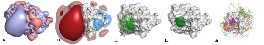
Figure 2: Sonic Hedgehog protein (Shh) with heparin ligand. (A) ESP isosurfaces of Shh at $+1$ $k_{\mathrm{B}}T/|e|$ (blue) and $-1$ $k_{\mathrm{B}}T/|e|$ (red). (B) EG isosurfaces at $\pm 1$ $k_{\mathrm{B}}T$ (translucent blue/red) and $\pm 2$ $k_{\mathrm{B}}T$ (solid blue/red), merging across two population-weighted conformations of a heparin di-saccharide (clustering details and glycosidic angles are provided in Table Supporting information) according to Equation 11. (C) EG based probability density of heparin di-saccharide drawn around 20% HDR (solid green) and 30% HDR (translucent green). The 20% HDR forms a hull around the crystallographic position of the heparin tetra-saccharide from ⁴⁷ (PDB entry 4c4n).(D) MD based probability density of heparin di-saccharide drawn at 20% and 30% HDR (solid and translucent green) from a 3.5 µs multi-trajectory MD simulation. (E) MD traces of the seven 500 ns simulations.

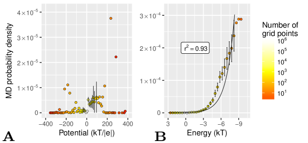
Figure 3: Probability density of heparin di-saccharide occupancy computed from MD simulations vs. electrostatic potential (A) and energy grid (B) at the same grid positions. Each point in the plot stands for all grid points with a certain value of potential (A) or energy (B), as given by its position along the horizontal axes. The number of grid points with the respective ESP or EG values are shown as colors. Both horizontal axes go from repulsive to attractive, and in both panels the vertical axes give the probability estimated by MD sampling, averaged over the grid points with a given ESP or EG value. The error bars mark the 99% confidence interval, assuming normally distributed probabilities. In panel A, thirteen outliers in the ESP grid with energies ranging from 400 to 800 $k_{\mathrm{B}}T/|e|$ lie outside the plotting range. Figure Supporting information shows the distribution in a 2D histogram.

3.2 C₅-epimerase and poly-anionic heparan sulfate substrates and non-substrates

D-glucuronyl C₅-epimerase modifies heparan sulfate (HS), i.e. long, negatively charged, and highly flexible carbohydrate chains. The epimerase has a varied surface topography with deep clefts. The HS chains have to be threaded through a narrow, partially buried active site, which makes the epimerase-HS complex a harder test case than the Shh-heparin complex of the previous section, where heparin bound preferentially to a well-accessible surface patch on Shh. The more specific, conformation dependent chemical function of the epimerase suggests a more accurate positioning of the HS substrate chains on epimerase than the superficial attachment of heparin to Shh. The hypothesis of a more accurate positioning is consistent with the observed substrate length dependency of the reaction: enzymatic activity decreased by 90% on a digested heparan sulfate fraction containing octasaccharides and smaller oligosaccharides ⁴⁸. Our question was therefore whether we would be able to trace an extended binding site in EGs that could accommodate such longer oligosaccharides. For validation we compared the predicted binding sites with crystallographically determined binding sites with a heparin inhibitor (PDB entry 4pxq ⁴⁹).

We used three different HS dimer fragments (Figure 4A) to compute the EGs: CH₃O-GlcNS-GlcA-OCH₃ as model of the substrate, CH₃O-GlcNS-IdoA-OCH₃ as model of the product, and CH₃O-GlcNAc-GlcA-OCH₃ as a non-substrate ^{48, 50}. Note that in vitro the enzyme works both ways, i.e. the product is a substrate for the reversed reaction ⁵⁰. A parsimonious, natural explanation of this finding is that substrate and product use the same molecular binding site.

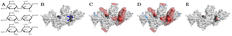
Figure 4: D-glucuronyl C₅-epimerase interaction with heparan sulfate. (A) di-saccharides used to compute EGs around epimerase. Top: substrate CH₃O-GlcNS-GlcA-OCH₃; middle: product and in vitro substrate CH₃O-GlcNS-IdoA-OCH₃; bottom: non-substrate CH₃O-GlcNAc-GlcA-OCH₃. (B) Crystal structure of epimerase in complex with heparin hexamer (PDB entry 4pxq ⁴⁹). The two heparin fragments (black) bind at the two active sites of the C₂ symmetric enzyme dimer. Amino acids critical for reaction (Ala-mutations lead to enzyme activity loss of >60% compared to wild-type ⁴⁹) are marked in blue. C–E: EGs of substrate (C), product (D), and non-substrate (E) scanned using the apo protein (PDB entry 4pw2 ⁴⁹) with isosurfaces drawn at $-1$ $k_{\mathrm{B}}T$ (translucent red) and $-2$ $k_{\mathrm{B}}T$ (solid red) and crystallographic heparin (black space filling). Isosurfaces in C–E were robust against changes of dihedral angles of the HS dimer used for scanning. Glycosidic angles are provided in Table Supporting information.

In fact, in the EGs with epimerase substrate and product we detected the same low energy channel, centered around the active sites (Figure 4B–D). The region that binds most strongly in the EG matches the crystallographic positions of the heparin hexasaccharide, and covers the amino acid residues most important for enzymatic activity ⁴⁹. However, the low energy region extends noticeably beyond the crystallographic location of the heparin hexasaccharide and could easily accommodate HS oligomers longer than octasaccharides (translucent red in Figure 4C,D). The shape of this low energy region suggests a core binding site for HS chains reaching from the right flank of the narrow cleft with the active center down the crystallographic heparin binding site.

While the substrate and product are both doubly negatively charged, the non-substrate molecule (bottom of Figure 4A) carries only one negative charge. In the corresponding EG the $-1$ $k_{\mathrm{B}}T$ region has shrunk drastically and now only covers the location of the crystallographic heparin hexasaccharide. Thus, although the non-substrate could be chemically epimerized in principle – it has the same GlcA amenable to epimerization – this particular epimerase enzyme offers no suitable binding site for a longer chain of this non-substrate type.

3.3 14-3-3 protein and poly-cationic supramolecular ligand

Recently we could demonstrate experimentally (Gigante et al., unpublished) that the binding of a supramolecular ligand, QQJ-096⁵¹ (Figure 5B), stabilizes the interaction between the 14-3-3 protein and peptide fragments of c-Raf protein (we call this complex 14-3-3/c-Raf). The large QQJ-096 ligand has three flexible arms (“R” in Figure 5B), each of them ending in two positively charged groups, a Lysine and Guanidinocarbonylpyrrole (GCP). The size and flexibility of the ligand makes it unsuitable for small molecule docking, and it is unlikely that this ligand takes a single, well-defined binding pose. Nevertheless its effect on the interaction of c-Raf and 14-3-3 could be explained most easily by a specific binding of QQJ-096 to 14-3-3/c-Raf.

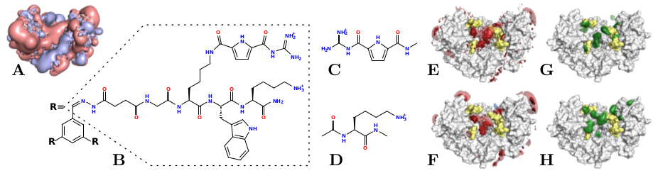
Figure 5: Interaction of 14-3-3/c-Raf complex with supramolecular ligand QQJ-096. (A) isosurfaces of electrostatic potential at $+1$ $k_{\mathrm{B}}T/|e|$ (blue) and $-1$ $k_{\mathrm{B}}T/|e|$ (red) of 14-3-3/c-Raf (PDB entry 4ihl ⁵²). (B) QQJ-096 ligand with only one of three arms (“R”) shown. (C) GCP with capped ends. (D) Lys with capped ends. (E and F) EG computed with Epitopsy for GCP and Lys, respectively, around 14-3-3/c-Raf. (G and H) 20% HDR (solid green) and 30% HDR (translucent green) for GCP and Lys, respectively, from a 1.5 µs multi-trajectory MD simulation of the 14-3-3/c-Raf with QQJ-096 in aqueous solution.

The electrostatics of 14-3-3/c-Raf shows many of regions of low electrostatic potential (red in Figure 5A) that could interact with the positive end groups of QQJ-096, Lys and GCP. For a more ligand-specific assessment of binding, we computed two EGs with molecules corresponding to the end groups of QQJ-096, GCP (Figure 5C) and Lys (Figure 5D). The EGs show roughly the same features for GCP (Figure 5E) and Lys (Figure 5F), with particularly high affinities in the center of the 14-3-3 cleft between the c-Raf peptides. For Lys there are additional high affinity patches so that the c-Raf fragments are sandwiched between regions of high affinity of Lys. Both end groups have a few small high affinity islands outside the central cleft of 14-3-3/c-Raf, with Lys having more of those islands than GCP. Overall, this result suggests that QQJ-096 could seal off the 14-3-3/c-Raf cleft and in this way inhibit dissociation of c-Raf fragments, in agreement with experimental results (Gigante et al., unpublished).

For comparison we simulated the 14-3-3/c-Raf/QQJ-096 system with MD. Considering the size of the molecular system and the low charge density on the ligand, a computational experiment analogous to the Shh-heparin experiment above seemed to be unfeasible, i.e. we do not expect to reach the MD steady state in the microsecond time scale with a ligand initially positioned at random in the solvent box. Based on the experimental evidence for a QQJ-096-mediated stabilization of the 14-3-3/c-Raf complex, and assuming a direct mode of interaction, the MD starting conditions can be narrowed down to the 14-3-3 cleft (Figure Supporting information). Based on this reasoning, we carried out a pilot set of six 50 ns MD simulations of the 14-3-3/c-Raf dimer in aqueous solution with QQJ-096 initially positioned 10 Å above the c-Raf peptides. In three simulations the ligand failed to interact with the protein. We then ran six 250 ns simulations with the ligand initially positioned 4–6 Å above the c-Raf peptides and observed a quick convergence to binding sites of QQJ-096 end groups in the 14-3-3 cleft matching those predicted by EGs computed with the end groups (Figure 5G,H). Regions outside the cleft were barely explored. Thus, MD simulations and EGs both support the same mechanism for the experimentally observed stabilization of the 14-3-3/c-Raf binding by QQJ-096, namely that the supramolecular ligand QQJ-096 blocks the 14-3-3 cleft and in this way impedes escape of c-Raf.

3.4 Kringle domain and flexible zwitterionic ligand

The Kringle domains of plasminogen attach to Lys residues on fibrin, a precondition for the decomposition of fibrin by plasminogen. A known alternative ligand of the Kringle domains is $\epsilonup$-aminocaproic acid (EACA), and a crystal structure of its complex with plasminogen Kringle domain 4 (KR4) has been determined (PDB entry 2pk4 ⁵³). EACA is a highly flexible, zwitterionic molecule (Figure 6A–C) that binds to a shallow basin in the KR4 surface. We have used the EACA-KR4 complex as a test case for the application of EGs based on multiple ligand conformers for the identification of binding sites (Equation 11). In an application scenario we would probably not know the actual conformer but rely on plausible ligand conformers obtained from other experiments or modeling. Accordingly, our EACA input conformers were the stretched conformer(Figure 6A) observed in the solid phase of pure EACA ⁵⁴, and a MM energy minimized turn geometry (Figure 6B) that is entropically and enthalpically more favorable for a free ligand. The conformer actually observed in the crystal complex (Figure 6C) is closer to the stretched geometry in the solid phase (Figure 6A), though with a bent amino-end.

The zwitterionic nature of EACA suggests a binding site that bridges two regions of opposite electrostatic potential. However, this pattern is too unspecific since there are many regions that fall into this category (Figure 6D). The full correlation with shape and electrostatics information leads to the identification of the correct binding basin, that, in fact, bridges regions of opposite electrostatic potential (Figure 6E–G). For the stretched EACA conformer there are two binding sites, the one in the crystal structure, and an alternative binding site with slightly lower affinity between Asp381 and Lys433 (Figure 6E). For the EACA turn conformer the correct basin is clearly the region with highest affinity (Figure 6F). The EG averaged over both ligand conformers (Equation 11, both ligand conformations weighted equally) also has the basin of the crystal structure as clearly dominating binding site (Figure 6G).

A question related to the multiconformer ligand treatment is the multiconformer receptor treatment, and Equation 11 treats ligand and receptor symmetrical in this respect. In fact, Figure 6G is based not only on two ligand conformations but also on three, equally weighted KR4 receptor conformations, including the EACA-KR4 complex structure 2pk4, a KR4 complex with sulfate (PDB entry 1krn), and a KR4 complex with arginine (PDB entry 4duu). However, since the differences between receptor structures are small (RMSDs to 2pk4: $0.29$ Å for 1krn and $0.69$ Å for 4duu on $\text{C}_{\alpha}$ atoms) the results are very similar for the combined EG and for the three EGs based on single receptor structures: For all three apo KR4 structures the respective EG identified the same correct EACA binding basin as best binding site.

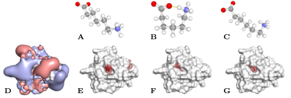
Figure 6: $\epsilonup$-aminocaproic acid (EACA) and its complex with plasminogen Kringle domain 4 (KR4). (A) Experimental structure (“stretched”) of EACA in the solid phase (CCDC entry 1102509⁵⁴). B: Energy-minimized structure of EACA (“turn”, MMFF94 forcefield, steepest descent in vacuum). (C) Structure of EACA in complex with KR4 (PDB entry 2pk4). (D) Electrostatic potential isosurfaces around apo KR4 (PDB entry 2pk4) drawn at $+1$ $k_{\mathrm{B}}T/|e|$ (blue) and $-1$ $k_{\mathrm{B}}T/|e|$ (red). E-G: EG isosurfaces a drawn at $\pm 1$ $k_{\mathrm{B}}T$ (translucent blue/red) and $\pm 2$ $k_{\mathrm{B}}T$ (solid blue/red) of apo KR4 with EACA stretched (E), as turn (F), and merging across multiple conformations of the ligand and protein according to Equation 11 (G).

4 Discussion

The very nature of large, flexible ligands, such as glycosaminoglycan chains, large receptor loops, or novel supramolecular binders, makes it challenging to model their interactions with proteins. First, these ligands are too large and flexible for small-molecule docking. Even the notion of a well-defined binding pose, commonly used in small-molecule docking, probably has to be abandoned. Instead, we should restate the aim from finding the binding pose to computing a probability density for the ligand around the protein. Second, the vastness of their conformational space makes large, flexible ligands also difficult objects for the standard method MD simulation, as it will be prone to severe undersampling ^{55, 56}. A third established candidate method is continuum electrostatics. It takes advantage of the charged nature of the ligands, but the electrostatic potential alone is difficult to interpret. The fact that electrostatics alone is not sufficient to locate large charged ligands like DNA or RNA has been noted before ^{57, 58}. Our results corroborate this because we found only a weak correlation between the electrostatic potential, the probability density obtained from extensive MD simulations of the Shh-heparin system, and corresponding experimental data. In this case we achieved good consistency with MD simulation and experimental structures with EGs that complement electrostatics with information about shape and volume of the ligand or ligand fragments.

The good correlation of the EG approach with probability densities from extensive MD simulations at a small fraction of the computational cost (typically CPU minutes vs. weeks) makes EGs an interesting way to approximate such densities. However, there are also limitations that should be considered. There are two basic categories of deficiencies: first, those due to features of the real system that are missing in the model, and second, those due to inadequate configuration of the model.

Intra-ligand interactions fall into the first category of deficiencies. In the fragment-based screening used for the EGs, we neglect interactions between fragments. This can be problematic since we are looking at large, flexible ligands that carry charges, and that can have plenty of opportunities for such interactions, e.g. repulsion between same sign charges, salt-bridges, or $\pi$-cation interactions. It is clear that such interaction exist, and that they can have an impact on the ligand structure⁵⁹. A factor that could limit the severity of the effect of intra-molecular interactions is that they have to compete with ligand-protein and ligand-water interactions, and with the conformational entropy of the ligand.

Another example of a principal deficiency of the underlying model is the use of continuum electrostatics. This leads e.g. to the neglect of structural water molecules, although such waters can be crucial for specific interactions at the surface of charged proteins ^{60, 61}. A similar argument can be made for ions. Inclusion of fixed water molecules or ions in the protein structure is technically feasible in EG computations. For a first tests we used the Trp repressor interaction with a nucleotide ligand where structural water molecules are known to mediate interactions ⁶². In this case the presence of the known structural water molecules had a negligible effect on the ligand distribution (Figure Supporting information).

Yet another deficiency is the treatment of molecular flexibility. In the case of the Kringle domain we have demonstrated that flexibility can be included both on the side of the protein and the side of the ligand fragments. However, the relevant conformations have to be known beforehand. If the protein-ligand interaction induces a new set of conformations, the distributions obtained from the EGs may be misleading. While this has not been an issue in the cases discussed above, it could be relevant for highly flexible or disordered proteins.

Finally, the FFT based correlation computation used in Epitopsy treats protein and ligand inconsistently: while the protein is modeled as uniform medium with a low dielectric constant, the ligand is treated as point charges in continuum water. For flexible charged ligands this approximation can be acceptable because they will be well-solvated and polarizable, but it could become inaccurate for ligands with a more rigid structures or non-polar regions.

The second category of deficiencies can be controlled by proper configuration of the model. For instance, if the protein or the ligand fragment used for the computation of the EG can assume several drastically different conformations and the user chooses only one of those conformations, this will in general lead to systematic deviations between the computed and true densities. This problem can be solved by inclusion of several conformations (Equation 11).

Another source of errors that can be controlled is the grid configuration. If spatial or angular grids are too coarse, regions around the protein that contribute to the EG will be missed. In the present study we have used fragments with the maximum size of a di-saccharide and a grid spacing of 0.8 Å, and the comparison with MD and experimental data showed that the results are reasonable for the given ligands and proteins. However, we expect that problems will arise with increasing ligand fragment size and ruggedness of protein topography (Figure Supporting information). For instance, the larger the ligand fragment and the deeper protein pockets, the more difficult it will be to map the protein-ligand interaction on the angular and spatial grid, because many fragment poses will lead to collisions and therefore be discarded. Another useful parameter in this context is the clash penalty $\delta$ (Equation 1). A weaker penalty will increase noise but has also the potential of making visible finer structures in EG or probability density (Figure Supporting information).

The correct charge of the ligand fragment is crucial, as shown in the epimerase example. However, the approach is robust against small variations in the charge distribution (see e.g. Figure Supporting information), so that resource-intensive QM-based methods for charge assignment may be substituted with MM forcefield charges.

An important point that has not been addressed in this work is heterogeneous ligand composition. In the presented examples we could infer the location of larger ligands from fragment probability densities because the large ligand had a rather homogeneous composition, e.g. it was a heparin poly-saccharide with negative charges on all di-saccharides, or a multi-branched ligand with positively charged GCP and Lys groups. However, such large ligands may comprise subunits of different physico-chemical characters. In this case information of EGs for different ligand fragments have to be combined to infer likely locations of complete ligands. We are currently developing methods to post-process sets of EGs for heterogeneous ligands in this sense.

We have argued in the beginning that current computational methods are not suitable for the treatment of large, flexible ligands or that their application is very expensive. Unfortunately, the same applies also to high-resolution experimental characterization by X-ray crystallography or NMR. This makes it all the more important to develop reliable and efficient computational methods that can e.g. be used to predict protein residues that are crucial for the interaction with the ligand. Such predictions can then be tested e.g. by measuring affinity changes after site-directed mutagenesis.

5 Author contribution

Conceived and designed the experiments: JNG DH. Performed the calculations: JNG. Analyzed the data: JNG LO DH. Contributed computational tools: JNG CW JND LO. Contributed experimental data: AG CS CO. Wrote the paper: JNG DH.

6 Competing interests

The authors of this manuscript have read the journal policy and declare that they have no competing interests.

This work was supported by Deutsche Forschungsgemeinschaft through grant CRC 1093 to CS and AG (subproject A1), JNG, LO, DH (subproject A7), and CO (subproject B4).

Supporting information

Table S1: Geometries of the glycosaminoglycans used as input for EGs. Figure S1: Initial placement of QQJ-096 in the MD simulations with 14-3-3/c-Raf. Table S2: Refined PDB structures. Figure S2: Effect of the number of rotations $\left|\mathbf{\Omega}\right|$. Figure S3: Effect of the grid resolution and penalty $\delta$. Figure S4: Effect of explicit water molecules. Figure S5: Effect of the ligand size. Figure S6: Effect of the ligand charge distribution. Figure S7: Binding/unbinding events in the heparin/Sonic Hedgehog MD simulations. Figure S8: 2D histograms of the ESP and EG vs. MD probability density.

References

- Capila and Linhardt 2002 Capila, I.; Linhardt, R. J. Heparin-protein interactions. Angewandte Chemie (International ed. in English) 2002, 41, 391–412
- Coombe and Kett 2005 Coombe, D. R.; Kett, W. C. Heparan sulfate-protein interactions: therapeutic potential through structure-function insights. Cellular and molecular life sciences : CMLS 2005, 62, 410–424
- Myszka et al. 2000 Myszka, D. G.; Sweet, R. W.; Hensley, P.; Brigham-Burke, M.; Kwong, P. D.; Hendrickson, W. A.; Wyatt, R.; Sodroski, J.; Doyle, M. L. Energetics of the HIV gp120-CD4 binding reaction. Proceedings of the National Academy of Sciences of the United States of America 2000, 97, 9026–9031
- Willcox et al. 1999 Willcox, B. E.; Gao, G. F.; Wyer, J. R.; Ladbury, J. E.; Bell, J. I.; Jakobsen, B. K.; van der Merwe, P. A. TCR binding to peptide-MHC stabilizes a flexible recognition interface. Immunity 1999, 10, 357–365
- Gilles et al. 2017 Gilles, P.; Wenck, K.; Stratmann, I.; Kirsch, M.; Smolin, D. A.; Schaller, T.; de Groot, H.; Kraft, A.; Schrader, T. High-Affinity Copolymers Inhibit Digestive Enzymes by Surface Recognition. Biomacromolecules 2017,
- Jiang et al. 2013 Jiang, Q. Q.; Bartsch, L.; Sicking, W.; Wich, P. R.; Heider, D.; Hoffmann, D.; Schmuck, C. A new approach to inhibit human -tryptase by protein surface binding of four-armed peptide ligands with two different sets of arms. Org Biomol Chem 2013, 11, 1631 – 1639
- Yu et al. 2014 Yu, W.; Lakkaraju, S. K.; Raman, E. P.; MacKerell, A. D. Site-Identification by Ligand Competitive Saturation (SILCS) assisted pharmacophore modeling. Journal of computer-aided molecular design 2014, 28, 491–507
- Goodford 1985 Goodford, P. J. A computational procedure for determining energetically favorable binding sites on biologically important macromolecules. Journal of medicinal chemistry 1985, 28, 849–857
- Katchalski-Katzir et al. 1992 Katchalski-Katzir, E.; Shariv, I.; Eisenstein, M.; Friesem, A. A.; Aflalo, C.; Vakser, I. A. Molecular surface recognition: determination of geometric fit between proteins and their ligands by correlation techniques. Proceedings of the National Academy of Sciences of the United States of America 1992, 89, 2195–2199
- Gabb et al. 1997 Gabb, H. A.; Jackson, R. M.; Sternberg, M. J. Modelling protein docking using shape complementarity, electrostatics and biochemical information. Journal of molecular biology 1997, 272, 106–120
- Kozakov et al. 2006 Kozakov, D.; Brenke, R.; Comeau, S. R.; Vajda, S. PIPER: an FFT-based protein docking program with pairwise potentials. Proteins 2006, 65, 392–406
- Brenke et al. 2009 Brenke, R.; Kozakov, D.; Chuang, G.-Y.; Beglov, D.; Hall, D.; Landon, M. R.; Mattos, C.; Vajda, S. Fragment-based identification of druggable ’hot spots’ of proteins using Fourier domain correlation techniques. Bioinformatics (Oxford, England) 2009, 25, 621–627
- Honig and Nicholls 1995 Honig, B.; Nicholls, A. Classical electrostatics in biology and chemistry. Science (New York, N.Y.) 1995, 268, 1144–1149
- Baker et al. 2001 Baker, N. A.; Sept, D.; Joseph, S.; Holst, M. J.; McCammon, J. A. Electrostatics of nanosystems: application to microtubules and the ribosome. Proceedings of the National Academy of Sciences of the United States of America 2001, 98, 10037–10041
- Pronk et al. 2013 Pronk, S.; Páll, S.; Schulz, R.; Larsson, P.; Bjelkmar, P.; Apostolov, R.; Shirts, M. R.; Smith, J. C.; Kasson, P. M.; van der Spoel, D.; Hess, B.; Lindahl, E. GROMACS 4.5: a high-throughput and highly parallel open source molecular simulation toolkit. Bioinformatics (Oxford, England) 2013, 29, 845–854
- Hornak et al. 2006 Hornak, V.; Abel, R.; Okur, A.; Strockbine, B.; Roitberg, A.; Simmerling, C. Comparison of multiple Amber force fields and development of improved protein backbone parameters. Proteins 2006, 65, 712–725
- Kirschner et al. 2008 Kirschner, K. N.; Yongye, A. B.; Tschampel, S. M.; González-Outeiriño, J.; Daniels, C. R.; Foley, B. L.; Woods, R. J. GLYCAM06: a generalizable biomolecular force field. Carbohydrates. Journal of computational chemistry 2008, 29, 622–655
- Homeyer et al. 2006 Homeyer, N.; Horn, A. H. C.; Lanig, H.; Sticht, H. AMBER force-field parameters for phosphorylated amino acids in different protonation states: phosphoserine, phosphothreonine, phosphotyrosine, and phosphohistidine. Journal of molecular modeling 2006, 12, 281–289
- Cieplak et al. 1995 Cieplak, P.; Cornell, W. D.; Bayly, C.; Kollman, P. A. Application of the multimolecule and multiconformational RESP methodology to biopolymers: Charge derivation for DNA, RNA, and proteins. Journal of Computational Chemistry 1995, 16, 1357–1377
- Frisch et al. 2009 Frisch, M. J. et al. Gaussian 09 Revision A.02. 2009; \urlhttp://www.gaussian.com
- Bayly et al. 1993 Bayly, C. I.; Cieplak, P.; Cornell, W.; Kollman, P. A. A well-behaved electrostatic potential based method using charge restraints for deriving atomic charges: the RESP model. The Journal of Physical Chemistry 1993, 97, 10269–10280
- Cornell et al. 1993 Cornell, W. D.; Cieplak, P.; Bayly, C. I.; Kollmann, P. A. Application of RESP charges to calculate conformational energies, hydrogen bond energies, and free energies of solvation. Journal of the American Chemical Society 1993, 115, 9620–9631
- Cornell et al. 1995 Cornell, W. D.; Cieplak, P.; Bayly, C. I.; Gould, I. R.; Merz, K. M.; Ferguson, D. M.; Spellmeyer, D. C.; Fox, T.; Caldwell, J. W.; Kollman, P. A. A Second Generation Force Field for the Simulation of Proteins, Nucleic Acids, and Organic Molecules. Journal of the American Chemical Society 1995, 117, 5179–5197
- Case et al. 2012 Case, D. A. et al. AMBER 12. 2012; \urlhttp://ambermd.org
- Sousa da Silva and Vranken 2012 Sousa da Silva, A. W.; Vranken, W. F. ACPYPE - AnteChamber PYthon Parser interfacE. BMC research notes 2012, 5, 367
- Berendsen et al. 1987 Berendsen, H. J. C.; Grigera, J. R.; Straatsma, T. P. The missing term in effective pair potentials. The Journal of Physical Chemistry 1987, 91, 6269–6271
- Bussi et al. 2007 Bussi, G.; Donadio, D.; Parrinello, M. Canonical sampling through velocity rescaling. The Journal of chemical physics 2007, 126, 014101
- Parrinello and Rahman 1981 Parrinello, M.; Rahman, A. Polymorphic transitions in single crystals: A new molecular dynamics method. Journal of Applied Physics 1981, 52, 7182–7190
- Páll and Hess 2013 Páll, S.; Hess, B. A flexible algorithm for calculating pair interactions on SIMD architectures. Computer Physics Communications 2013, 184, 2641–2650
- Darden et al. 1993 Darden, T.; York, D.; Pedersen, L. Particle mesh Ewald: An N.log(N) method for Ewald sums in large systems. The Journal of Chemical Physics 1993, 98, 10089–10092
- Hess et al. 1997 Hess, B.; Bekker, H.; Berendsen, H. J. C.; Fraaije, J. G. E. M. LINCS: A linear constraint solver for molecular simulations. Journal of Computational Chemistry 1997, 18, 1463–1472
- Team and R Foundation for Statistical Computing 2016 Team, R. C.; R Foundation for Statistical Computing, R: A Language and Environment for Statistical Computing. 2016
- Hyndman 1996 Hyndman, R. J. Computing and Graphing Highest Density Regions. The American Statistician 1996, 50, 120–126
- Schrödinger 2015 Schrödinger, L. L. C.
- Webb and Sali 2014 Webb, B.; Sali, A. Protein Structure Modeling with MODELLER; Springer New York: New York, NY, 2014; Chapter 1, pp 1–15, removed editor=Kihara, Daisuke
- Eswar et al. 2001 Eswar, N.; Webb, B.; Marti-Renom, M. A.; Madhusudhan, M. S.; Eramian, D.; Shen, M.-y.; Pieper, U.; Sali, A. Comparative Protein Structure Modeling Using MODELLER; John Wiley & Sons, Inc., 2001
- Dolinsky et al. 2007 Dolinsky, T. J.; Czodrowski, P.; Li, H.; Nielsen, J. E.; Jensen, J. H.; Klebe, G.; Baker, N. A. PDB2PQR: expanding and upgrading automated preparation of biomolecular structures for molecular simulations. Nucleic acids research 2007, 35, W522–W525
- Dolinsky et al. 2004 Dolinsky, T. J.; Nielsen, J. E.; McCammon, J. A.; Baker, N. A. PDB2PQR: an automated pipeline for the setup of Poisson-Boltzmann electrostatics calculations. Nucleic acids research 2004, 32, W665–W667
- Singh and Kollman 1984 Singh, U. C.; Kollman, P. A. An approach to computing electrostatic charges for molecules. Journal of Computational Chemistry 1984, 5, 129–145
- Besler et al. 1990 Besler, B. H.; Merz, K. M.; Kollman, P. A. Atomic charges derived from semiempirical methods. Journal of Computational Chemistry 1990, 11, 431–439
- Gasteiger and Marsili 1978 Gasteiger, J.; Marsili, M. A new model for calculating atomic charges in molecules. Tetrahedron Letters 1978, 19, 3181 – 3184
- Gasteiger and Marsili 1980 Gasteiger, J.; Marsili, M. Iterative partial equalization of orbital electronegativity – a rapid access to atomic charges. Tetrahedron 1980, 36, 3219–3228
- O’Boyle et al. 2011 O’Boyle, N. M.; Banck, M.; James, C. A.; Morley, C.; Vandermeersch, T.; Hutchison, G. R. Open Babel: An open chemical toolbox. Journal of cheminformatics 2011, 3, 33
- Wilms 2013 Wilms, C. Methods for the Prediction of Complex Biomolecular Structures. 2013; \urlhttp://duepublico.uni-duisburg-essen.de/servlets/DerivateServlet/Derivate-34803/BIB_Thesis_Christoph_Wilms.pdf
- Swinbank and James Purser 2006 Swinbank, R.; James Purser, R. Fibonacci grids: A novel approach to global modelling. Quarterly Journal of the Royal Meteorological Society 2006, 132, 1769–1793
- González 2009 González, Á. Measurement of Areas on a Sphere Using Fibonacci and Latitude–Longitude Lattices. Mathematical Geosciences 2009, 42, 49
- Whalen et al. 2013 Whalen, D. M.; Malinauskas, T.; Gilbert, R. J. C.; Siebold, C. Structural insights into proteoglycan-shaped Hedgehog signaling. Proceedings of the National Academy of Sciences of the United States of America 2013, 110, 16420–16425
- Jacobsson et al. 1984 Jacobsson, I.; Lindahl, U.; Jensen, J. W.; Rodén, L.; Prihar, H.; Feingold, D. S. Biosynthesis of heparin. Substrate specificity of heparosan N-sulfate D-glucuronosyl 5-epimerase. The Journal of biological chemistry 1984, 259, 1056–1063
- Qin et al. 2015 Qin, Y.; Ke, J.; Gu, X.; Fang, J.; Wang, W.; Cong, Q.; Li, J.; Tan, J.; Brunzelle, J. S.; Zhang, C.; Jiang, Y.; Melcher, K.; Li, J.-p.; Xu, H. E.; Ding, K. Structural and functional study of D-glucuronyl C5-epimerase. The Journal of biological chemistry 2015, 290, 4620–4630
- Lindahl et al. 1989 Lindahl, U.; Kusche, M.; Lidholt, K.; Oscarsson, L. G. Biosynthesis of heparin and heparan sulfate. Annals of the New York Academy of Sciences 1989, 556, 36–50
- Jiang et al. 2015 Jiang, Q.-Q.; Sicking, W.; Ehlers, M.; Schmuck, C. Discovery of potent inhibitors of human beta-tryptase from pre-equilibrated dynamic combinatorial libraries. Chem. Sci. 2015, 6, 1792–1800
- Molzan et al. 2013 Molzan, M.; Kasper, S.; Röglin, L.; Skwarczynska, M.; Sassa, T.; Inoue, T.; Breitenbuecher, F.; Ohkanda, J.; Kato, N.; Schuler, M.; Ottmann, C. Stabilization of physical RAF/14-3-3 interaction by cotylenin A as treatment strategy for RAS mutant cancers. ACS chemical biology 2013, 8, 1869–1875
- Wu et al. 1991 Wu, T. P.; Padmanabhan, K.; Tulinsky, A.; Mulichak, A. M. The refined structure of the epsilon-aminocaproic acid complex of human plasminogen kringle 4. Biochemistry 1991, 30, 10589–10594
- Bodor et al. 1967 Bodor, G.; Bednowitz, A. L.; Post, B. The crystal structure of -aminocaproic acid. Acta Crystallographica 1967, 23, 482–490
- Neale et al. 2014 Neale, C.; Hsu, J. C. Y.; Yip, C. M.; Pomès, R. Indolicidin binding induces thinning of a lipid bilayer. Biophysical journal 2014, 106, L29–L31
- Nemec and Hoffmann 2017 Nemec, M.; Hoffmann, D. Quantitative Assessment of Molecular Dynamics Sampling for Flexible Systems. Journal of chemical theory and computation 2017, 13, 400–414
- Jones et al. 2003 Jones, S.; Shanahan, H. P.; Berman, H. M.; Thornton, J. M. Using electrostatic potentials to predict DNA-binding sites on DNA-binding proteins. Nucleic acids research 2003, 31, 7189–7198
- Chen and Lim 2008 Chen, Y. C.; Lim, C. Predicting RNA-binding sites from the protein structure based on electrostatics, evolution and geometry. Nucleic acids research 2008, 36, e29
- Lavery et al. 2014 Lavery, R.; Maddocks, J. H.; Pasi, M.; Zakrzewska, K. Analyzing ion distributions around DNA. Nucleic acids research 2014, 42, 8138–8149
- Materese et al. 2009 Materese, C. K.; Savelyev, A.; Papoian, G. A. Counterion atmosphere and hydration patterns near a nucleosome core particle. Journal of the American Chemical Society 2009, 131, 15005–15013
- Davey et al. 2002 Davey, C. A.; Sargent, D. F.; Luger, K.; Maeder, A. W.; Richmond, T. J. Solvent mediated interactions in the structure of the nucleosome core particle at 1.9 a resolution. Journal of molecular biology 2002, 319, 1097–1113
- Otwinowski et al. 1988 Otwinowski, Z.; Schevitz, R. W.; Zhang, R. G.; Lawson, C. L.; Joachimiak, A.; Marmorstein, R. Q.; Luisi, B. F.; Sigler, P. B. Crystal structure of trp repressor/operator complex at atomic resolution. Nature 1988, 335, 321–329