Theory for frequent measurements of spontaneous emissions in non-Markovian environment: beyond Lorentzian spectrum

Abstract

The measurement-result-conditioned evolution of a system (e.g. an atom) with spontaneous emissions of photons is well described by the quantum trajectory (QT) theory. In this work we generalize the associated QT theory from infinitely wide bandwidth Markovian environment to the case of finite bandwidth non-Markovian environment. In particular, we generalize the treatment for arbitrary spectrum, which is not restricted by the specific Lorentzian case. We rigorously prove a general existence of a perfect scaling behavior jointly defined by the bandwidth of environment and the time interval between successive photon detections. For a couple of examples, we obtain analytic results to facilitate QT simulations based on the Monte-Carlo algorithm. For the case where analytical result is not available, numerical scheme is proposed for practical simulations.

I introduction

In quantum mechanics, the theory of quantum measurement is based on the Copenhagen’s postulate of wave-function collapse conditioned on a specific outcome of measurement of an observable. Later generalization of the measurement theory, largely related to some indirect coupling and/or taking into account the realistic microscopic degrees of freedom of the apparatus,

has been more generally formulated as some POVM forms NC00 . In quantum optics, for continuous measurement, the theory has also been formulated as quantum trajectory (QT) and has found potential applications WM09 ; Jac14 ; Dali92 ; WM93 . In recent years, the QT theory has been applied as well to experiments in superconducting solid-state circuits Pala10 ; DiCa13 ; Hof11 ; Mar11 ; Dev13 ; Sid13 ; Sid12 ; DiCa12 ; Dev13a .

Actually, the existing QT theory is based on quantum measurements in Markovian (wide bandwidth) environments. A generalization of the QT theory for continuous measurements performed in non-Markovian (finite bandwidth) environment was recently proposed Xu16 , where the non-Markovian environment was modeled by using a Lorentzian spectral density function (SDF) with bandwidth ($\Lambda$), and perfect “scaling” property was found between the spectral bandwidth and and the measurement time interval ($\tau$), in terms of the scaling variable $x=\Lambda\tau$ SG14 . This generalization bridges the gap between the existing QT theory WM09 ; Jac14 and the Zeno effect, by rendering them as two extremes corresponding to $x\to\infty$ and $x\to 0$, respectively.

Therefore, a question on how we extend the continuous measurement theory to more general non-Markovian environment beyond the Lorentzian SDF, along with the question regarding the possibility of generally finding and proving the $x=\Lambda\tau$ scaling behavior. In the present work, we provide an investigation for this problem. The work is organized as follows. In Sec. II we present a numerical scheme to calculate the null-results conditioned state evolution, where the numerical accuracy is examined by comparing with the analytic results of the Lorentzian SDF, before carrying out the numerical results in Sec. III for three non-Lorentzian examples. Here perfect scaling behavior is first observed and then rigorously proved for general case. In Sec. IV we outline the Monte-Carlo algorithm and display the simulation results of quantum trajectories. Finally, we summarize the work with discussions in Sec. V.

II Formulation and Method

Let us consider a two-level atom coupled to electromagnetic vacuum (environment), which is described by the Hamiltonian

$$H=\frac{\Delta}{2}\sigma_{z}+\sum_{r}\left(b^{\dagger}_{r}b_{r}+\frac{1}{2}\right)\omega_{r}+\sum_{r}\left(V_{r}b^{\dagger}_{r}\sigma^{-}+{\rm H.c.}\right)\,.$$ (1)

Throughout this work we set $\hbar=1$. Here we introduce: the two-level energy difference $\Delta=E_{e}-E_{g}$, the atomic operators $\sigma_{z}=|e\rangle\langle e|-|g\rangle\langle g|$, $\sigma^{-}=|g\rangle\langle e|$, and $\sigma^{+}=|e\rangle\langle g|$. $V_{r}$ is the radiative coupling of the atom to the environment. Let us consider the evolution of the entire system, starting with an initial state $|\Psi(0)\rangle=(\alpha_{0}|e\rangle+\beta_{0}|g\rangle)\otimes|{\rm vac}\rangle$, where $|{\rm vac}\rangle$ stands for the environmental vacuum with no photon. Under the influence of coupling, the entire state at time $t$ can be expressed as

$$|\Psi(t)\rangle = \alpha(t)|e\rangle\otimes|{\rm vac}\rangle+\sum_{r}c_{r}(t)|g\rangle\otimes|1_{r};0;{\cdots}\rangle$$ (2)

$$+\,\beta_{0}|g\rangle\otimes|{\rm vac}\rangle\,,$$

where $|1_{r};0;{\cdots}\rangle$ describes the environment with a photon excitation in the state “$r$” and no excitations of other states. The coefficients have initial conditions of $\alpha(0)=\alpha_{0}$ and $c_{r}(0)=0$.

Substituting Eq. (2) into the Schrödinger equation, $i\partial_{t}|\Psi(t)\rangle=H|\Psi(t)\rangle$ and performing the Laplace transformation, $\tilde{f}(\omega)=\int_{0}^{\infty}f(t)\exp(i\omega t)dt$, we obtain the following system of algebraic equations:

$$(\omega-E_{e})\tilde{\alpha}(\omega)-\sum_{r}V_{r}\tilde{c}_{r}(\omega)=i\alpha_{0}\,,$$ (3a)

$$[\omega-(E_{g}+\omega_{r})]\tilde{c}_{r}(\omega)-V^{*}_{r}\tilde{\alpha}(\omega)=0\,.$$ (3b)

The r.h.s. of the first equation reflects the initial condition. Substituting $\tilde{c}_{r}(\omega)$ from Eq. (3b) into Eq. (3a), we obtain

$$(\omega-E_{e})\tilde{\alpha}(\omega)-{\cal F}(\omega)\tilde{\alpha}(\omega)=i\alpha_{0}\,.$$ (4)

In this result, we have introduced

$$\mathcal{F}(\omega)=\int\frac{D(\omega_{r})}{\omega-(E_{g}+\omega_{r})}\,d\omega_{r}\,,$$ (5)

where the spectral density function (SDF) was defined as usual as

$$D(\omega_{r})=\sum_{r^{\prime}}|V_{r^{\prime}}|^{2}\delta(\omega_{r}-\omega_{r^{\prime}})\,.$$ (6)

Rather than the wide-band limit required for the “Markovian” reservoir, in this work we consider a finite-band spectrum. For Lorentzian SDF, as shown in Ref.Xu16 , we can first solve Eq. (4) in frequency domain, then obtain the analytic solution of $\alpha(t)$ by means of inverse-Laplace transformation. However, for arbitrary SDF $D(\omega_{r})$, this strategy does not work. Instead, we can solve Eq. (4) for $\alpha(t)$ numerically in time domain. For this purpose, an inverse-Laplace transformation to Eq. (4) yields

$$\dot{\alpha}(t)=-iE_{e}\,\alpha(t)-i\int_{0}^{t}du\,F(u)\,\alpha(t-u)\,,$$ (7)

where the kernel function in the integral in time domain is the inverse Laplace transformation of ${\cal F}(\omega)$, which reads

$$F(u)=-i\,\int d\omega_{r}D(\omega_{r})\,e^{-i(\omega_{r}+E_{g})u}\,.$$ (8)

In obtaining this result, we have used the following identity

$$\int^{\infty}_{-\infty}\frac{d\omega}{2\pi}\,\frac{e^{-i\omega u}}{\omega-(\omega_{r}+E_{g})}=-i\,e^{-i(\omega_{r}+E_{g})u}\,.$$ (9)

It would be desirable to eliminate the energy ($E_{e}$) caused phase factor and the initial condition $\alpha(t=0)=\alpha_{0}$. Let us introduce the decay factor of the excited state $a(t)$, via $\alpha(t)=\alpha_{0}e^{-iE_{e}t}a(t)$, and introduce as well $\tilde{F}(u)=F(u)e^{iE_{e}u}$. We have

$$\dot{a}(t)=-i\int_{0}^{t}du\,\tilde{F}(u)\,a(t-u)\,.$$ (10)

In practice, for a given SDF $D(\omega_{r})$, one can first carry out $\tilde{F}(u)$ in advance, then numerically integrate Eq. (10) to obtain $a(t)$ using a discretized algorithm as follows

$$a(Ndt)=a[(N-1)dt]-i\,dt\left(\sum_{j=1}^{N}\tilde{F}(jdt)a[(N-j)dt]\,dt\right)$$ (11)

Here $N\,dt=t$, with $dt$ a discretized increment of time interval.

II.1 Lorentzian Spectrum: Analytic Solution

Let us consider first the Lorentzian SDF which allows analytic solution. The Lorentzian SDF is assumed as

$$D(\omega_{r})=D_{0}\Lambda^{2}/[(\omega_{r}-\omega_{0})^{2}+\Lambda^{2}]\,,$$ (12)

where $\omega_{0}$ is the spectral center, $D_{0}$ the spectral height and $\Lambda$ the spectral width. Substituting this SDF into Eq. (5), we obtain

$$\mathcal{F}(\omega)={\Lambda\Gamma/2\over(\omega-\omega_{0}-E_{g})+i\Lambda},~{}~{}{\rm where}~{}~{}\Gamma=2\pi D_{0}\,.$$ (13)

Based on this result, one can solve Eq. (4) first for $\tilde{\alpha}(\omega)$ in the frequnecy domain, then perform an inverse Laplace transform, $\alpha(t)=\int_{-\infty}^{\infty}\tilde{\alpha}(\omega)e^{-i\omega t}d\omega/(2\pi)$. Taking into account the convention $\alpha(t)=a(t)\alpha_{0}e^{-iE_{e}t}$, one obtains the decay factor SG14

$$a(t)={1\over A_{+}-A_{-}}(A_{+}e^{-A_{-}t}-A_{-}e^{-A_{+}t})\,,$$ (14)

where $A_{\pm}=[\Lambda-iE\pm\sqrt{(\Lambda-iE)^{2}-2\Gamma\Lambda}]/2$, and the energy offset $E=(E_{e}-E_{g})-\omega_{0}$.

Let us now consider to introduce frequent projective measurements of photon in the reservoir, with time intervals $\tau$. We may have two possible results: a photon registered by the detector; or no photon detected, i.e., a null result of measurement. For the first case, the atom jumps to its ground state. For the case of null result, the atom state would also have a change by excluding the second term with one photon in the reservoir from Eq. (2). At this moment, we are interested in the case of $n$ successive null results of measurements. Conditioned on this, the atom state at $t=n\tau$ should be

$$|\Psi_{A}(t)\rangle=\left([a(\tau)]^{n}\alpha_{0}|e\rangle+\beta_{0}|g\rangle\right)/{\cal N}\,,$$ (15)

where ${\cal N}$ denotes a normalization factor.

We may further consider the limit of “continuous” measurements, $n\to\infty$ by taking the measurement time interval $\tau\to 0$ and keeping $t=n\tau$ fixed. Supposing to increase the bandwidth $\Lambda$ so that the variable $x=\Lambda\tau$ remains constant, we can prove a “scaling” property that the final state becomes a function of $x$ only. To be a little bit more general, we also assume the energy offset $E=c\Lambda$ (in usual treatment $c=0$). After simple manipulations, we arrive to SG14

$$\bar{a}(t)=[a(\tau)]^{n}=\exp\left\{-\left[\frac{1}{\kappa}-(1-e^{-\kappa x})\frac{1}{\kappa^{2}x}\right]\frac{\Gamma t}{2}\right\}\,,$$ (16)

where $\kappa=1-ic$. Elegantly, this effective decay factor reveals an explicit scaling property in the $x=\Lambda\tau$-variable.

II.2 Accuracy Examination

For non-Lorentzian SDF, it may not be possible to obtain analytic solution as above for the Lorentzian spectrum. However, instead, one can carry out numerical results. Before applying the numerical method to several examples, we would like first to examine it by comparison with the analytic solution under Lorentzian spectrum. The key quantity for numerical computation is the kernel function $\tilde{F}(u)$, which should be obtained in advance. For the Lorentzian SDF, this kernel function can be easily obtained as

$$\tilde{F}(u) = -i\,\int d\omega_{r}D(\omega_{r})\,e^{-i(\omega_{r}+E_{g}-E_{e})u}$$ (17)

$$= -i\,(\Gamma\Lambda/2)e^{i(E_{e}-E_{g}-\omega_{0})u}e^{-\Lambda u}\,.$$

With this, one can solve for $a(t)$ from Eq. (10), i.e., numerically from the iterative expression Eq. (11). In Fig. 1(a), for atom initially in $\alpha_{0}|e\rangle+\beta_{0}|g\rangle$ and later subject to the influence of spontaneous emission (coupling to environment), we show the decay probability of the component $|e\rangle$, $|a(t)|^{2}$. We compare the results based on the numerical Eq. (11) and from the analytic solution Eq. (14), respectively, for spectral bandwidths $\Lambda=100\Gamma$, $10\Gamma$, $5\Gamma$ and $\Gamma$. In Fig. 1(b), we further compare the results of the decay probability of $|e\rangle$, conditioned on null-results of frequent measurements with time interval $\tau$. In the numerical calculation, we adopt $\Lambda=5\Gamma$ and a couple of $\tau$ resulting in thus $x=\Lambda\tau=2$, 0.2 and 0.02. We compare the results against the analytic solution of Eq. (16) which are obtained under the limits $\Lambda\to\infty$ and $\tau\to 0$. The full agreement of the results shown in Fig. 1(a) and (b) demonstrate that the numerical method proposed above is efficient and precise enough, which can be safely applied to the non-Lorentzian spectrum where analytic solution may not be available.

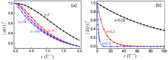
Figure 1: Accuracy examination of the numerical method via comparison with the analytic solution under Lorentzian spectrum. (a) Decay probability of the excited state $|e\rangle$, under the influence of spontaneous emission (coupling to environment) but without intermediate interruptions of frequent null-result measurements. The dots are from the numerical Eq. (11) while the lines from the analytic solution Eq. (14). (b) Decay probability of $|e\rangle$ conditioned on the frequent null-result measurements. The dots are from numerical calculation based on Eq. (11) and $\bar{a}(t)|_{t=n\tau}=[a(\tau)]^{n}$, by adopting $\Lambda=5\Gamma$ and a couple of $\tau$ so that $x=\Lambda\tau=2$, 0.2 and 0.02. The lines display the analytic solution of Eq. (16) under the limits $\Lambda\to\infty$ and $\tau\to 0$. We also assumed $E_{e}-E_{g}=\omega_{0}$.

III Numerical Results and General Scaling Behavior

In this section we apply Eq. (10) or (11) to several non-Lorentzian examples. We will consider in particular the null-results conditioned evolution under continuous measurement, which is a key ingredient for the construction of quantum trajectories. That is, assuming $\alpha_{0}=1$ (initially the atom on the excited state $|e\rangle$), we will compute the survival probability $P_{e}(t)=|\bar{a}(t)|^{2}$, where $t=n\tau$ and $\bar{a}(t)=[a(\tau)]^{n}$. Numerically, we obtain $a(\tau)$ from Eq. (10).

Also, based on the numerical results, we will first explore the existence of scaling behavior, then rigorously prove it for arbitrary SDF.

III.1 Three Models

Let us consider the following three models of non-Lorentzian SDF.

These models may approximately describe possible real systems but here they are largely used for mathematical purposes. As we will see soon, these specific models allow us to obtain analytic expressions of $\tilde{F}(u)$ which can guide us to find a property necessarily needed to prove the interesting scaling behavior. However, we will prove subsequently that the scaling behavior holds for arbitrary SDF, not depending on any specific forms such as the models we assume here.

The first example is a Gaussian SDF given by

$$D(\omega_{r})=D_{0}e^{-\frac{(\omega_{r}-\omega_{0})^{2}}{2\Lambda^{2}}}\,.$$ (18)

Accordingly, we obtain the kernel function in Eq. (10) as

$$\tilde{F}(u)=-i\,\frac{\Gamma\Lambda}{\sqrt{2\pi}}e^{i(E_{e}-E_{g}-\omega_{0})u}e^{-\Lambda^{2}u^{2}}\,,$$ (19)

where $\Gamma=2\pi D_{0}$.

The second example we will consider is a constant SDF with finite bandwidth, given by

$$D(\omega_{r})=\left\{\begin{aligned} &D_{0},\,\,&|\omega_{r}-\omega_{0}|\leq\Lambda/2\\ &0,\,\,&|\omega_{r}-\omega_{0}|>\Lambda/2\end{aligned}\right.\,.$$ (20)

For this model, the corresponding kernel function reads

$$\tilde{F}(u)=-i\,\frac{\Gamma}{\pi u}e^{i(E_{e}-E_{g}-\omega_{0})u}\sin(\Lambda u/2)\,.$$ (21)

Here we also defined $\Gamma=2\pi D_{0}$.

The third example is a double-Lorentzian SDF

$$D(\omega_{r})=\sum_{j=1,2}\frac{D_{0}\Lambda^{2}}{\Lambda^{2}+[\omega_{r}-\omega_{0}+(-1)^{j}\omega_{1}]^{2}}\,.$$ (22)

Similarly, we obtain the kernel function as

$$\tilde{F}(u)=-i\,\Gamma\Lambda e^{i(E_{e}-E_{g}-\omega_{0})u}e^{-\Lambda u}\cos(\omega_{1}u)\,.$$ (23)

We defined as well $\Gamma=2\pi D_{0}$.

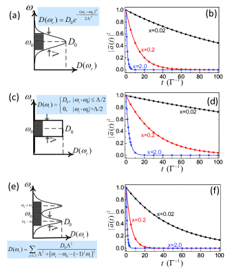
Figure 2: Frequent null-results conditioned decay of $|e\rangle$ under coupling to environment with non-Lorentzian spectrum. Three examples of SDF are schematically shown in (a), (c) and (e), while the corresponding results are displayed, respectively, in (b), (d) and (f). For each given $x$, different $\Lambda$ (and accordingly $\tau$) are chosen, e.g., $\Lambda=100\Gamma$ (lines) and $5\Gamma$ (dots) as shown here.

III.2 Numerical Results

In Fig. 2 we plot the results for the three non-Lorentzian examples. That is, for each SDF, we show the null-results conditioned decay probability of $|e\rangle$, i.e., $|\bar{a}(t=n\tau)|^{2}=|a^{n}(\tau)|^{2}$ . We plot results for three parameters $x=2.0$, 0.2 and 0.02. We observe that the decay is slowed down as we reduce $x$, as a consequence of the Zeno effect. This is because by noting that $x=\Lambda\tau$, for a fixed $\Lambda$, smaller $x$ simply means smaller $\tau$ (i.e. more frequent measurements). More interesting observation is that, for a given $x$ but quite different $\Lambda$ (e.g., $\Lambda=100\Gamma$ and $5\Gamma$ as we compare in Fig. 2), the null-results conditioned evolution is identical under varying $\Lambda$ and accordingly $\tau$, as shown in Fig. 2 by the perfect coincidence of the dots and the lines. This clearly reveals a remarkable ‘scaling’ behavior, with $x=\Lambda\tau$ the scaling variable.

Qualitatively, we may understand the scaling behavior as follows, by means of the time-energy uncertainty principle. According to the uncertainty principle, the measurements with time interval $\tau$ will disturb the atomic level of $|e\rangle$ by an energy fluctuation of $\tau^{-1}$. Then, for more frequent measurements (smaller $\tau$), if we expand as well the spectral width $\Lambda$ of the reservoir to keep $x=\Lambda\tau$ unchanged (see the examples schematically plotted in Fig. 2), the atomic decay (spontaneous emission) is seemingly not to be affected by the stronger energy fluctuations ($\sim\tau^{-1}$) with respect to the reservoir spectrum. However, it is still somehow surprising that the scaling behavior governed by $x=\Lambda\tau$ is so precise, as shown in Fig. 2 by the perfect coincidence between the dots and curves. It would be of great interest to investigate further, more quantitatively, the underlying reason.

III.3 Proof of Scaling Behavior

In our previous work Xu16 ; SG14 , restricted in the Lorentzian SDF, we have proven an exact scaling property via obtaining the analytic expression Eq. (16), under the ‘continuous’ limit $\tau\to 0$ (meanwhile making $\Lambda\to\infty$). For non-Lorentzian case, however, the analytic solution of $a(t)$ such as Eq. (14) is not available. Below we present a different proving method, which is applicable to broader cases.

To fulfill such a proof, a key observation is that, for all the examples illustrated above, the rescaled $\tilde{F}(u)/\Lambda$ is a function of the joint parameter $x=\Lambda u$. We may formally denote it as

$$\tilde{F}(u)/\Lambda=g(x)\,.$$ (24)

Note that here we have involved the consideration $E=c\Lambda$, while $E\equiv E_{e}-E_{g}-\omega_{0}$ is the offset of the transition energy from the spectral center. Also, in Eq. (23) for the double-Lorentzian SDF, the locations of the peak centers are proportional to the peak width, i.e., $\omega_{1}\propto\Lambda$.

Starting with Eq. (10), let us consider the evolution over $(0,\tau)$. For the limit $\tau\to 0$, we can replace $a(\tau-u)$ in the integrand by $a(\tau)$, yielding

$$\dot{a}(\tau)=-i\int_{0}^{\tau}du\,\tilde{F}(u)\,a(\tau)\,.$$ (25)

The physical meaning of this procedure is that, in short time limit, the non-Markovian memory effect is not relevant. For this time-local differential equation, the solution simply reads $a(\tau)=e^{Q(\tau)}$. We further evaluate $Q(\tau)$ as follows:

$$Q(\tau) = -i\int_{0}^{\tau}du^{\prime}\int_{0}^{u^{\prime}}du^{\prime\prime}\tilde{F}(u^{\prime\prime})$$ (26)

$$= -\,\frac{i\tau}{x}\int_{0}^{x}dx^{\prime}\int_{0}^{x^{\prime}}dx^{\prime\prime}g(x^{\prime\prime})\,.$$

Here we have introduced $x=\Lambda\tau$, $x^{\prime}=\Lambda u^{\prime}$ and $x^{\prime\prime}=\Lambda u^{\prime\prime}$. Based on this result, we can easily obtain the successive null-results conditioned evolution as

$$\bar{a}(t)=a^{n}(\tau)=e^{nQ(\tau)}=e^{-\gamma(x)\,t/2}\,.$$ (27)

Here we have used $t=n\tau$, and the effective decay rate is given by

$$\gamma(x)=i\,\frac{2}{x}\int_{0}^{x}dx^{\prime}\int_{0}^{x^{\prime}}dx^{\prime\prime}g(x^{\prime\prime})\,.$$ (28)

This result fully proves the scaling property of the null-results conditioned evolution. The mathematical rigorousness is based on the key structure of Eq. (24), i.e., $\tilde{F}(u)/\Lambda=g(\Lambda u)$.

Then, the most interesting question is that this structure can be valid in general for arbitrary SDF? We now extend our consideration to general case. Actually, for an arbitrary form of SDF $D(\omega_{r})$, we can rewrite it as $D(\omega_{r})=\tilde{D}(\omega_{r}-\omega_{0})$, with $\omega_{0}$ close to or simply equal to the atomic transition energy. Then, as schematically shown in Fig. 3, let us consider a series of deformation of this SDF i.e., $\tilde{D}(\omega_{r}-\omega_{0})$, by varying its “width” $\Lambda$ in accordance with the change of the detection time interval $\tau$, in order to keep $x=\Lambda\tau$ fixed. Notice that, for an arbitrary form of SDF, it may not necessarily have a natural width parameter $\Lambda$ in its functional form. In order to describe the whole class of deformed curves of the SDF as shown in Fig. 3 (and explained above), we can simply introduce a width parameter $\Lambda$ to the SDF, as $\tilde{D}(\frac{\omega_{r}-\omega_{0}}{\Lambda})$. That is, via varying $\Lambda$ in this function, we can obtain all the deformed SDFs as schematically shown in Fig. 3. Now let us re-denote this class of SDF by $D(\omega_{r},\Lambda)$, i.e., $D(\omega_{r},\Lambda)\equiv\tilde{D}(\frac{\omega_{r}-\omega_{0}}{\Lambda})$. Obviously, this general consideration renders the SDF with a “natural” width parameter (as numerically demonstrated in the previous subsections) as special examples of this general form. Then, we manipulate the proving as follows:

$$\tilde{F}(u)=-i\,\int d\omega_{r}\,D(\omega_{r},\Lambda)\,e^{-i(\omega_{r}+E_{g}-E_{e})u}$$

$$=-i\,\int d\omega_{r}\,\tilde{D}(\frac{\omega_{r}-\omega_{0}}{\Lambda})\,\,e^{-i[(\omega_{r}-\omega_{0})-(E_{e}-E_{g}-\omega_{0})]u}$$

$$=-i\Lambda\int d\omega\tilde{D}(\omega)e^{-i(\omega-c)(\Lambda u)}$$

$$\equiv\Lambda\,g(\Lambda u)\,.$$ (29)

Here, as done previously, we have assumed $E_{e}-E_{g}-\omega_{0}\equiv E=c\Lambda$. In this way we proved the general structure of $\tilde{F}(u)/\Lambda=g(\Lambda u)$, which can guarantee the scaling behavior of the null-result conditioned evolution as proved through Eqs. (25)-(28).

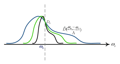
Figure 3: Deformation of the spectral-density-function (SDF) via introducing a changeable width parameter $\Lambda$, in order to keep $x=\Lambda\tau$ fixed when changing the detection time interval $\tau$.

We would like to mention that, instead of the short-time-limit treatment as Eq. (25), an alternative treatment following Ref. Kur00 can result in the $x=\Lambda\tau$ scaling behavior as well, provided that the property proved by Eq. (III.3) is valid as it is. Moreover, as proved in Appendix A, both limiting treatments give essentially the same result of Eq. (28). In Ref. Kur00 , rather than the scaling behavior concerned here, the main interest was concentrated on the Zeno and anti-Zeno effects, by considering only the change/decrease of $\tau$ but with $\Lambda$ unchanged. The anti-Zeno effect occurs for some special SDF when speeding the successive measurements (reducing the interval $\tau$), manifested as acceleration of decay in certain intermediate range of $\tau$. As an interesting addition, in the above, we generally proved that even for the anti-Zeno SDF analyzed in Ref. Kur00 , the decay rate will be exactly the same –not influenced by speeding the measurements– if we alter $\Lambda$ as well to keep $x=\Lambda\tau$ unchanged.

We may further carry out the explicit expressions of $\gamma(x)$ for the examples we illustrated. Before that, we first examine the Lorentzan SDF Eq. (12). Straightforwardly, from Eq. (28), we obtain

$$\gamma(x)=\Gamma\left[\frac{1}{\kappa}-(1-e^{-\kappa x})\frac{1}{\kappa^{2}x}\,\right]$$ (30)

where $\kappa=1-ic$ and $c$ is introduced from $E=c\Lambda$. Desirably, based on this different method (i.e. not solving $a(t)$ to get Eq. (14) previously), we obtain the same result of Eq. (16).

Now, for the Gaussian SDF shown in Fig. 2(a), we obtain

$$\gamma(x)=\Gamma\left[{\rm erf}\left(\frac{x}{\sqrt{2}}\right)+\frac{2}{\sqrt{2\pi}x}\left(e^{-\frac{x^{2}}{2}}-1\right)\right]\,,$$ (31)

where ${\rm erf(x)}=\int_{0}^{x}e^{-x^{2}}dx$ is the Error function. For simplicity, here and for the other two non-Lorentzian examples, we assume $E_{e}-E_{g}=\omega_{0}$ (thus $c=0$). For nonzero $c$, analytic expressions are also available but more complicated in form. The results of the other two examples are, respectively, for the rectangular SDF (Fig. 2 (c))

$$\gamma(x)=\frac{2\Gamma}{\pi}\left[{\rm Si}(\frac{x}{2})+\frac{2}{x}\cos\frac{x}{2}-\frac{2}{x}\right]\,,$$ (32)

where ${\rm Si}(x)=\int_{0}^{x}\frac{\sin x}{x}dx$; and for the Double-Lorentzian SDF (Fig. 2(e))

$$\gamma(x)=\Gamma\left(1-\frac{e^{-x}\sin x}{x}\right)\,.$$ (33)

In addition to $c=0$, in this last example we also assumed $b=1$ with $b$ defined from $\omega_{1}=b\Lambda$.

IV Quantum trajectories

We now turn to constructing a practical scheme for quantum trajectory (QT) simulation, associated with continuous measurement (photon detection) in a non-Markovian environment and beyond Lorentzian SDF for the atom-environment coupling. It is well known that the existing QT theory is associated with continuous measurements in wide-band-limit Markovian environment WM09 ; Jac14 ; Dali92 ; WM93 . From the fundamental theoretical viewpoint, the existing QT theory has an imperfection that its prediction differs from the quantum Zeno effect, as explained in detail in Ref. Xu16 . It would thus be very desirable to develop a unified description to quantitatively bridge the gap between the QT theory and the Zeno physics. This problem has been addressed in our recent studies Xu16 ; SG14 , where the consideration was restricted within the finite-bandwidth Lorentzian SDF. Using Lorentzian SDF, the available analytic solution allows not only proving the scaling behavior, but also constructing the QT approach based on the effective emission rate associated with frequent detection of photons.

Below we extend the quantum trajectory study beyond the Lorentzian SDF, by applying Eq. (10) or (11), or more efficiently, Eq. (27) to calculate the null-results conditioned evolution under continuous measurement, which is a key ingredient for the construction of quantum trajectories. In order to simulate the quantum trajectories, let us consider also to introduce optical drive to the atom. Conditioned on the results of measurement, one can then construct a Monte-Carlo wave function approach, closely following the line of the standard quantum trajectory theory for measurements in Markovian environment Dali92 ; WM93 ; WM09 ; Jac14 .

Specifically, let us consider the evolution over the time interval $(t,t+\Delta t)$. To construct an efficient theory for the successive photon detections with shorter time intervals $\tau$, one can utilize the accumulated result over $\Delta t=n\tau$ to perform a one-step update for the atom state. This longer time duration, $\Delta t$, is roughly determined from the criterion that during $\Delta t$ there is at most one photon registered in the detector Dali92 ; WM93 ; WM09 ; Jac14 . Therefore, during $\Delta t$, there will be two possible outcomes: a photon registered in the detectors ($\Delta N_{c}=1$), or no photon registered ($\Delta N_{c}=0$). In the former case, we simply update the atom state by a jump action; while for the latter result the atom takes an effective smooth (but non-unitary) evolution.

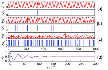
Figure 4: Quantum trajectories, taking the rectangular SDF shown in Fig. 2(c) as an example, are displayed for $x=0.02$, 0.2 and 2 in (a), (b) and (c), respectively. The events of photon emissions are also shown by plotting $\Delta N_{c}=1$ resulted from the Monte-Carlo simulation. In (d), for $x=0.2$, the ensemble-average over 5000 trajectories is compared against the result from the Lindblad master equation with photon emission rate $\gamma_{\rm eff}$. For all the results here, the Rabi parameter $\Omega$ in the driving Hamiltonian $\Omega\sigma_{x}$ is adopted as $\Omega=\Gamma$.

To perform Monte-Carlo simulations, during $\Delta t$, the probability with a photon registered in the detectors is $p^{(n)}_{1}(\Delta t)=|\alpha(t)|^{2}\gamma_{\rm eff}\Delta t$. Here we denote the effective emission rate under frequent detections by $\gamma_{\rm eff}$, which is given by

$$\gamma_{\rm eff}=[1-|\bar{a}(\Delta t)|^{2}]/\Delta t\,.$$ (34)

For small $\Delta t$ and for the form of Eq. (27), we simply have $\gamma_{\rm eff}={\rm Re}\gamma(x)$, as given by Eqs. (31), (32) and (33), respectively, for the examples we illustrated.

In practical simulations, generate a random number $\epsilon$ between 0 and 1. If $\epsilon<p^{(n)}_{1}(\Delta t)$, which corresponds to the probability of having a photon registered in detectors ($\Delta N_{c}=1$), we update the state by a “jump” action. Otherwise, the atom experiences a smooth evolution. Including together the evolution caused by the optical drive, we can update the atom state in a compact way formally expressed as

$$|\Psi_{A}(t+\Delta t)\rangle={\cal U}(\Delta t){\cal M}_{1,0}(\Delta t)|\Psi_{A}(t)\rangle\,/\parallel\bullet\parallel\,,$$ (35)

where $\parallel\bullet\parallel$ denotes the normalization factor. ${\cal U}(\Delta t)$ describes the unitary evolution owing to the optical drive, while ${\cal M}_{1,0}(\Delta t)$ are the Krause operators in the POVM formalism which read, respectively, ${\cal M}_{1}(\Delta t)=\sigma^{-}$ for $\Delta N_{c}=1$, and ${\cal M}_{0}(\Delta t)=diag\{\bar{a}(\Delta t),1\}$ for $\Delta N_{c}=0$. Note also that the above form of ${\cal M}_{0}(\Delta t)$ is associated with expressing the atom state $|\Psi_{A}(t)\rangle=\alpha(t)|e\rangle+\beta(t)|g\rangle$ in terms of a column vector $[\alpha(t),\beta(t)]^{T}$, which makes well defined the action of ${\cal M}_{0}(\Delta t)$ on the atom state.

Taking the rectangular SDF shown in Fig. 2(c) as an example, we display in Fig. 4 the results of quantum trajectory simulations, based on the Monte-Carlo algorithm proposed above. In Fig. 4(a), (b) and (c) we show, respectively, a single representative trajectory for $x=0.02$, 0.2 and 2; and for each case we indicate also the events of photon emissions. We observe that, for smaller $x$ (smaller $\tau$), the photo emissions are scarcer. This is nothing but the consequence of the Zeno effect. This phenomenon can be observed only for photon-detection in finite-bandwidth non-Markovian environment. For wide-band-limit Markovian environment, the results are independent of $\tau$ SG13 ; WM09 ; Jac14 ; Dali92 ; WM93 .

In Fig. 4(d), for $x=0.2$ as an example, we show the result of ensemble-average over 5000 trajectories and compare it with the result from an ensemble-averaged master equation, say, the Lindblad master equation with photon emission rate of $\gamma_{\rm eff}$. We find perfect agreement between them. We may remark that, the average result shown in Fig. 4(d) is not the usual reduced dynamics after tracing out the degrees of freedom of the environment, despite that tracing means also averaging all the measurement results. But the average associated with the reduced state is done only at the concerned time instant $t$; before $t$, there are no measurement interruptions – as involved in contrast by the quantum trajectory simulation – to the entangled evolution of the coupled system-and-environment.

More detailed discussion about this issue is referred to Ref. Xu16 and references therein (the series of works by Wiseman et al).

V Discussion and Summary

In the existing QT theory and simulations, the time step $\Delta t$ is assumed such that during $\Delta t$ there is at most one photon emitted/detected, while the (smaller) measurement time interval $\tau$ is implied to account for the continuous (or, frequent) measurements. To our knowledge, it has not been well clarified that the existing QT result is free from the choice of $\tau$ SG13 . This implies that, in the existing QT theory, the choice of the measurement interval $\tau$ can be relaxed to $\Delta t$ SG13 . However, our result, which is associated with finite bandwidth $\Lambda$ and small measurement time interval $\tau$, shows that the result depends on the choice of $\tau$. For instance, different choice of $\tau$ can result in big differences such as dynamical phase transition in the counting statistics of spontaneous emissions XL16 .

On the other aspect, if we let the interval $\tau=\Delta t$, this defines the scaling parameter $x=\Lambda\,\Delta t$. Owing to the scaling property, for not very narrow $\Lambda$ and not long $\Delta t$, we cannot distinguish the result from the one given by different $\Lambda$ and $\tau$ but with the same $x$ ($x=\Lambda\tau$). Only for very narrow bandwidth $\Lambda$ and relatively long $\Delta t$, the result differs from that given by the same $x$ under choice of large $\Lambda$ and small $\tau$. However, for any cases, Eq. (10) is a good starting point for the QT simulations. For the former case, the non-Markovian memory effect is killed by the frequent interruptions of measurement, which reduce the solution of Eq. (10) to the simpler result of Eq. (25), or Eqs. (27) and (28). For the latter case, the memory-involved iteration based on Eq. (11) can be implemented.

Generally speaking, the finite bandwidth environment will result in memory effect in the reduced dynamics of the system of interest. This is typically manifested by a time-convolutional form of master equation for the reduced state, just as observed also in Eq. (10). In this sense, we call the environment with finite bandwidth a non-Markovian one. However, in the presence of frequent measurement interruptions, the non-Markovian memory effect is largely destroyed. The main consequence of the non-Markovian (finite bandwidth) environment is the dependence of the measurement interval $\tau$, or more interestingly, of the scaling variable $x=\Lambda\tau$.

To summarize, we have generalized the measurement theory and the associated QT approach to environment with finite bandwidth and beyond the Lorentzian spectrum. For finite $\Lambda$ and small $\tau$, which results in a finite or small parameter $x=\Lambda\tau$, the null-result conditioned state evolution and quantum jump probability will be drastically affected by the choice of $\tau$, or more interestingly, by the scaling parameter $x$.

For arbitrary SDF, we generally proved the existence of scaling property. For Lorentzian and some non-Lorentzian SDFs, by keeping $x=\Lambda\tau$ fixed but making the limits $\Lambda\to\infty$ and $\tau\to 0$, we obtained analytic result to facilitate the QT simulation for finite $\Lambda$ and $\tau$ (but with the same $x$), owing to the underlying scaling property.

However, even if the analytical result is not available, one can still use Eq. (11) or Eqs. (27) and (28) to simulate the quantum trajectories.

Acknowledgements.

— This work was supported by the National Key Research and Development Program of China (No 2017YFA0303304), and the National Natural Science Foundation of China(No 11675016).

Appendix A Connection with the KK Solution

In this Appendix we make a connection of our treatment leading to Eqs. (27) and (28) with the Kofman-Kurizki (KK) solution of Eq. (12) in Ref. Kur00 , which was employed there to analyze the Zeno and anti-zeno effects. Starting with Eq. (10), i.e., $\dot{a}(\tau)=-i\int^{\tau}_{0}du\tilde{F}(u)a(\tau-u)$, following Ref. Kur00 , in the limit of short $\tau$ we alternatively have

$$\dot{a}(\tau)\simeq-i\int^{\tau}_{0}du\tilde{F}(u)\,.$$ (36)

Here the limit consideration $\alpha(\tau-u)\rightarrow\alpha(0)=1$ in the integrand was inserted. This consideration has a formal difference from the one leading to Eq. (25) in the main part of this work. Nevertheless, we will find both treatments equivalent.

Integrating the both sides of Eq. (36) we obtain

$$a(\tau)-a(0) = -i\int^{\tau}_{0}du\left[\int^{u}_{0}du^{\prime}\tilde{F}(u^{\prime})\right]$$ (37)

$$= -i\int^{\tau}_{0}\mathrm{d}u\,(\tau-u)\tilde{F}(u)\,.$$

In deriving the second equality we have used the technique of integration by parts. Actually this is the KK solution Eq. (10) given in Ref. Kur00 .

Now let us consider $\bar{a}(t)=[a(\tau)]^{n}$ in the short-$\tau$-limit under the condition $t=n\tau$. Noting that $a(0)=1$, we have

$$[a(\tau)]^{n} = \left[1-i\int^{\tau}_{0}du\,(\tau-u)\tilde{F}(u)\right]^{n}$$ (38)

$$\simeq 1-i\,n\int^{\tau}_{0}du\,(\tau-u)\tilde{F}(u)$$

$$= 1-i\,t\int^{\tau}_{0}du\,(1-u/\tau)\tilde{F}(u)$$

$$\simeq e^{-rt/2}\,.$$

In the result of the last line, the following rate parameter was introduced

$$r=2i\int_{0}^{\tau}du\,(1-u/\tau)\tilde{F}(u)\,.$$ (39)

The real part of this quantity, say, $R=\mathrm{Re}(r)$, gives rise to the result of Eq. (12) in Ref. Kur00 . Notice that, in Ref. Kur00 , $P_{e}(t=n\tau)=|a(\tau)|^{2n}\simeq e^{-Rt}$ was interpreted as the survival probability under frequent observations in the context of Zeno effect, while in our present work $[a(\tau)]^{n}$ is inserted into Eq. (15) as a null-results conditioned change of the superposition amplitude which is in general a complex number.

Below we employ Eq. (39) to prove the scaling property, with the help of the key structure observed by Eq. (24) and proved in general by Eq. (III.3). As in the main part, let us introduce the scaling parameters $x=\Lambda\tau$ and $x^{\prime}=\Lambda u$. We then reexpress Eq. (39) as follows:

$$r = 2i\,\int_{0}^{x^{\prime}/\Lambda}d(x^{\prime}/\Lambda)\,(1-x^{\prime}/x)\tilde{F}(x^{\prime}/\Lambda)$$ (40)

$$= \frac{2i}{x}\int_{0}^{x}dx^{\prime}\,(x-x^{\prime})g(x^{\prime})\,\equiv\,r(x)\,,$$

which shows that $r$ is a function of the joint variable $x=\Lambda\tau$, i.e., holding the desired scaling property. We should emphasize that, in order to achieve the proving, using here the property $\tilde{F}(x^{\prime}/\Lambda)=\Lambda g(x^{\prime})$ proved in Eq. (III.3) is a key point.

We now prove that this result is nothing but the one given by Eq. (28), which is obtained in the main part by a different limiting treatment. Starting with Eq. (28), the proving simply reads:

$$\gamma(x) = \frac{2i}{x}\int_{0}^{x}dx^{\prime}\int_{0}^{x^{\prime}}dx^{\prime\prime}\,g(x^{\prime\prime})$$ (41)

$$= \frac{2i}{x}\left[x\int^{x}_{0}\mathrm{d}x^{\prime\prime}g(x^{\prime\prime})-\int^{x}_{0}x^{\prime}g(x^{\prime})\mathrm{d}x^{\prime}\right]$$

$$= \frac{2i}{x}\left[x\int^{x}_{0}\mathrm{d}x^{\prime}g(x^{\prime})-\int^{x}_{0}x^{\prime}g(x^{\prime})\mathrm{d}x^{\prime}\right]$$

$$= \frac{2i}{x}\int^{x}_{0}\mathrm{d}x^{\prime}\,(x-x^{\prime})g(x^{\prime})\,.$$

This is the result of $r(x)$ given by Eq. (40).

References

- (1) M. A. Nielsen and I. L. Chuang, Quantum computation and quantum information (Cambridge Univ. Press, Cambridge, 2000).
- (2) H. M. Wiseman and G. J. Milburn, Quantum Measurement and Control (Cambridge Univ. Press, Cambridge, 2009).
- (3) K. Jacobs, Quantum Measurement Theory and Its Applications (Cambridge Univ. Press, Cambridge, 2014).
- (4) J. Dalibard, Y. Castin, and K. Molmer, Phys. Rev. Lett. 68, 580 (1992).
- (5) H. M. Wiseman and G. J. Milburn, Phys. Rev. A 47, 642 (1993).
- (6) A. Palacios-Laloy, F. Mallet, F. Nguyen, P. Bertet, D. Vion, D. Esteve and A. N. Korotkov, Nat. Phys. 6, 442 (2010).
- (7) J. P. Groen, D. Risté, L. Tornberg, J. Cramer, P. C. de Groot, T. Picot, G. Johansson, and L. DiCarlo, Phys. Rev. Lett. 111, 090506 (2013)
- (8) A. J. Hoffman, S. J. Srinivasan, S. Schmidt, L. Spietz, J. Aumentado, H. E. Tureci, and A. A. Houck, Phys. Rev. Lett. 107, 053602 (2011).
- (9) M. Mariantoni et al., Nat. Phys. 7, 287 (2011).
- (10) M. Hatridge, S. Shankar, M. Mirrahimi, F. Schackert, K. Geerlings, T. Brecht, K. M. Sliwa, B. Abdo, L. Frunzio, S. M. Girvin, R. J. Schoelkopf, and M. H. Devoret, Science 339, 178 (2013).
- (11) K. W. Murch, S. J. Weber, C. Macklin and I. Siddiqi, Nature 502, 211 (2013).
- (12) R. Vijay, C. Macklin, D. H. Slichter, S. J. Weber, K. W. Murch, R. Naik, A. N. Korotkov and I. Siddiqi, Nature 490, 77 (2012).
- (13) D. Risté, J. G. van Leeuwen, H. S. Ku, K. W. Lehnert, and L. DiCarlo, Phys. Rev. Lett. 109, 050507 (2012).
- (14) P. Campagne-Ibarcq, E. Flurin, N. Roch, D. Darson, P. Morfin, M. Mirrahimi, M. H. Devoret, F. Mallet, and B. Huard, Phys. Rev. X 3, 021008 (2013)
- (15) L. Xu and X. Q. Li, Phys. Rev. A 94, 032130 (2016).
- (16) L. Xu, Y. Cao, X. Q. Li, Y. J. Yan, and S. Gurvitz, Phys. Rev. A 90, 022108 (2014).
- (17) J. Ping, Y. Ye, X. Q. Li, Y. J. Yan, and S. Gurvitz, Phys. Lett. A 377, 676 (2013).
- (18) L. Xu and X. Q. Li, Sci. Rep 8, 531 (2018).
- (19) A. G. Kofman and G. Kurizki, Nature (London) 405, 546 (2000).