Quantitative Classification of Type I Supernovae Using Spectroscopic Features at Maximum Brightness

Abstract

We present a set of new quantitative classification criteria for major subclasses of Type I Supernovae (SNe). We analyze peak spectra of 146 SNe Ia from the Berkeley Supernova Ia Program (BSNIP), 12 SNe Ib, 19 SNe Ic (including 5 SNe Ic-BL) and 4 SNe Ib/c. All the spectra are within 5 days of maximum light. We study their absorption line depths relative to the pseudo-continuum at around observed wavelength $\lambda$6150Å, attributed to Si II $\lambda$6355Å for SNe Ia and Ic and to hydrogen for SNe Ib, and O I $\lambda 7774$Å observed around $\lambda 7500$Å. We found that Type I SNe could be quantitatively classified using the line depths at these two absorption regions. Type Ia SNe, including normal SNe Ia, Ia-1991bg and Ia-1999aa, show strong signatures of Si II near peak with relative line depth values of $a{\rm(\lambda 6150\AA)>0.35}$. Only SNe Ia-2002cx (Iax) do not satisfy this criterion, while the $a{\rm(O\ I\ \lambda 7774\AA)}$ index can separate SNe Ia-1991bg and Ia-1999aa cleanly. Type Ib SNe satisfy that $a{\rm(\lambda 6150\AA)<0.35}$ and $a{\rm(\lambda 6150\AA)}/a{\rm(O\ I\ \lambda 7774\AA)>1}$, while regular Type Ic SNe show $a{\rm(\lambda 6150\AA)<0.35}$ but $a{\rm(\lambda 6150\AA)}/a{\rm(O\ I\ \lambda 7774\AA)<1}$. These quantitive classification criteria work well for the majority of normal Type I SN subclasses. Peculiar SNe Ia-2002cx and SNe Ic-BL are the exception. We apply these criteria to provide clear identifications to intermediate or unclear SNe Ib/c. The results show good consistency with classification using specific spectral line features. Though there are still some puzzles about the physical mechanisms driving the diverse line ratios, our method is an accurate empirical method to identify the majority of Type I SNe.

1 INTRODUCTION

The classification of SNe has been a systematic and long-lasting problem for astronomers since the middle of the 20th century. The first classification of SNe, based on spectroscopic data, was introduced by Minkowski (1941). Minkowski’s well-known classification criterion is that those SNe whose spectra show prominent signatures of Hydrogen were classified as Type II SNe, while Type I SNe did not show evidence for Hydrogen in their spectra.

After this first influential step, the following decades witnessed the introduction of several new SN subclasses. Among the Hydrogen-deficient Type I SNe, a new subclass of SNe Ib was noticed and differentiated from the dominant group (SNe Ia) by Wheeler & Levreault (1985) and Elias et al. (1985). Later Harkness et al. (1987) identified signatures of He I in peak spectra of SNe Ib and Wheeler & Harkness (1990) introduced the term SN Ic for a subclass of SNe Ib that did not show strong Helium absorption but were otherwise similar to SNe Ib (and different from SNe Ia).

During the last 20 years, with the rapid development of observation and data reduction techniques as well as the launch of several ambitious SN survey projects, a number of Type I SNe with peculiar photometric properties or spectroscopic features have been discovered, leading to the establishment of several subclasses, for instance, SN Ia 1991bg-like events whose prototype was first described by Filippenko et al. (1992), SN Ia 2002cx-like events, initially presented by Li et al. (2003) and discussed in detail in Foley et al. (2013) and White et al. (2015), as well as broad-line Type Ic SN events (Ic-BL), showing extreme values of velocity dispersion at and before peak which cause individual spectral lines to blend together (e.g. Mazzali et al., 2000; Xu et al., 2013; Modjaz et al., 2016). Some SNe Ic-BL events attract a lot of attention due to their association with high-energy GRB events (for a review see Woosley & Bloom, 2006). All of these discoveries enhance the diversity of Type I SNe, while a connection with the physical mechanism of SN explosion remains elusive. An updated review of SN classification is presented in Gal-Yam (2016).

The studies of Nugent et al. (2011) and Bloom et al. (2012) of the SN Ia 2011fe constrain the size of its progenitor, making a compact white dwarf (WD) the most likely progenitor star. However, the detailed physical scenario of these explosive events still remains an open question. Meanwhile, we have strong evidence that normal Type Ib and Ic SNe originate from massive progenitor stars (e.g. van Dyk, 1992; Smartt, 2009). The study of the SN Ib iPTF13bvn pre-explosion imaging, presented by Cao et al. (2013) as well as Fremling et al. (2014), shows an apparent massive progenitor and directly demonstrates the physical origin of SNe Ib. Direct evidence of the progenitors of SNe Ic is still missing. From similar spectral features shared with SNe Ib as well as host galaxy population and locations, it is widely believed that SNe Ic are also the result of the core collapse of massive stars.

Historically, SNe are classified by spectroscopic features (Filippenko, 1997; Gal-Yam, 2016). For example, SN Ia spectra around maximum light are characterized by conspicuous absorption around $\lambda$6150Å, which is produced by blueshifted Si II $\lambda$6355Å, while this feature is weak in SN Ib and Ic spectra (Wheeler et al., 1995). SNe Ib are defined by displaying strong He I $\lambda\lambda\lambda$5876Å 6678Å 7065Å absorption lines in near-peak spectra. These events also show an absorption line near $\lambda$6150Å whose nature is still debated (Parrent et al., 2016; Liu et al., 2016). Normal SNe Ic are overall similar to SNe Ib but by definition they do not show the three strong characteristic He I features near peak.

However, there still exist some problems with these traditional and well-developed classification criteria. The first issue is that this classification is not quantitative, due to many historical reasons. The definition of Type I SNe is based on unquantified spectroscopic distinctions (i.e, whether silicon and helium absorption lines exist or not) around their peak luminosity. Though such an empirical criterion works well for most conditions, it is often subjective or controversial (see Section 2.2.2 and 4.3). Meanwhile, the present definition of SNe Ic is based on lack of prominent hydrogen and helium features. Such a negative definition leaves a question whether all objects that are not SNe Ia, Ib or II belongs to the Type Ic class. In order to distinguish SNe Ic from other SNe accurately, we have to give a positive definition of this class.

Furthermore, the nature of some Type I SN spectroscopic features is still not confirmed. In particular, the absorption near $\lambda$6150Å in SN Ib spectra seems to be associated with H$\alpha$ (Parrent et al., 2016; Liu et al., 2016), while it may be due to Si II in SN Ic peak spectra.

Therefore, our goal in this project is to find a quantitative classification criterion for Type I SNe, just like William Wilson Morgan, Philip C. Keenan and Edith Kellman have done in 1943 to introduce the Yerkes stellar spectral classification (Morgan et al., 1943). One option is to use the line depth technique introduced by Silverman et al. (2012a). By measuring line depths of indicative lines, we aim to classify these SNe with a quantitative criterion on their absolute or relative line intensity, with different types located at different positions on a diagram. While there are many absorption lines that could probably play the role of indicators in SN spectra, we find that the conspicuous absorption lines near $\lambda$6150Å as well as O I $\lambda 7774$ Å can be found in almost every peak spectrum of Type I SNe. A preliminary result is presented in Gal-Yam (2016) and shows these two absorption lines may be good indicators, however, the sample size in that work is fairly small.

Here we plan to present a robust result that Type I SNe can be reclassified using the line depths of OI $\lambda 7774$ Å and the absorption at $\lambda 6150$ Å in rest wavelength around their maximum light. The SN spectra sample we adopted consists of 146 SNe Ia (including 3 SNe 2002cx-like, 1 SN 1991T-like, 21 SNe 1991bg-like, 8 SNe 1999aa-like and a single other unclassified peculiar object, namely SN2000cx), 12 SNe Ib, 19 SNe Ic (including 5 SNe Ic-BL objects) and 4 SNe Ib/c spectra around their maximum light respectively. Compared to the preliminary result mentioned above, we have increased the sample size by an order of magnitude. All the SNe Ia we utilized in this paper are from the Berkeley Supernova Ia Program (BSNIP), while some of their corresponding maximum-light time or peak spectra are from other publications. All public SNe Ib and Ic peak spectra can be found on the Weizmann Interactive Supernova data REPository (WISeREP, Yaron & Gal-Yam, 2012). We include data for several PTF objects kindly provided in advance of publication (Fremling et al., in preparation).

In Section 2 of this paper, we introduce the SN sample in detail and describe our selection criteria. The analysis methods we employed are presented in Section 3. Results are then presented and discussed in Section 4.

2 Supernovae Data

2.1 SNe Ia

Though the total number of SN Ia discoveries is quite large, we only use BSNIP objects in this paper. The reasons we chose BSNIP are as follows.

First, BSNIP events are all located in low-redshift galaxies, which means at relatively low distances and thus probably have higher quality spectra. In addition, these SNe Ia are well-studied objects. Among the 582 SN Ia objects presented in Silverman et al. (2012b), 199 have well-calibrated light curves, which can provide accurate phase information to 584 spectra. Since we want to study the spectroscopic features of Type I SNe at maximum light, it is crucial to know their dates of maximum. In addition, BSNIP spectra also have robust and uniform flux calibration and telluric correction.

In this paper, the major source of object subclasses and maximum dates is Silverman et al. (2012b). Each Type Ia SN subtype is directly adopted from the BSNIP I data release. 132 of the total 146 SN Ia spectra we utilized are also from BSNIP I. Phase information for 584 spectra has been provided in that paper. We combined this set with other papers studying SN Ia light curves, for example, Blondin et al. (2012), Stritzinger et al. (2011), as well as Krisciunas et al. (2011) which studies one specific SN Ia (SN2001ay), and enlarge the sample size of BSNIP SN Ia peak dates. All the maximum dates are with respect to B-band maximum brightness in rest-frame days.

After assembling a large sample of BSNIP SNe Ia with maximum dates, we match them to the observation dates of spectra in BSNIP I. The quality cut criteria are as follows:

1. The rest wavelength range of each spectrum should cover the range from 5800Å to 7800Å, which contains both of the absorption regions we will measure.
2. The observation date of each spectrum should fall within 5 days prior to or later than B-band maximum. This is our definition of peak spectra in this paper.
3. If there are more than a single peak spectrum for a specific object, we will only use the one taken closest to its B-band maximum brightness. If the closest one is of fairly low Signal to Noise Ratio (SNR), we will turn to the second closest one and inspect its quality to decide whether we adopt it or not, and so on.
4. If there are no corresponding peak spectra in the BSNIP I spectra package, we will turn to WISeREP to find whether there are other peak spectra in this database. The quality cut criteria are the same as 1 to 3 listed above.

After this step we find that 146 SNe Ia have corresponding peak spectra which can satisfy all the criteria listed above. Table 1 shows subtype, observation date and phase information of each SN Ia object we utilize in this paper.

Totally there are 6 subtypes for SNe Ia in Table 1, including 114 normal Ia (referred to as “SN Ia” in the table; containing SN2005ao and SN2008s5, whose subtypes remain undetermined), 1 Ia-1991T, 19 Ia-1991bg, 8 Ia-1999aa, 3 Ia-2002cx and 1 Ia-pec, following the classifications by Silverman et al. (2012b). SNe Ia-1999aa were classified as Ia-1991T objects in some previous publications (e.g. Li et al., 2001a) and these two subtypes show a great similarity in spectra except for Ca II H&K absorption and Si II $\lambda$6355Å line depth before maximum (Garavini et al., 2004). Due to this reclassification, the sample size of Ia-1991T objects has been sharply cut down. The Ia-pec subtype only contain SN2000cx, which is pointed out to be peculiar in its light curve features and spectral evolution properties (Li et al., 2001b; Silverman et al., 2013).

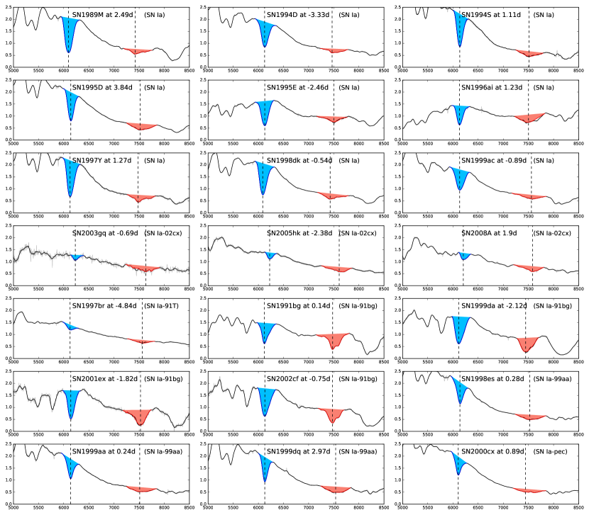
Figure 1: This figure shows 21 SN Ia spectra around their maximum light. In each subplot, the silver solid line (mostly covered by the black solid line) is the original spectrum (without smoothing, telluric line correcting and fitting), while the black solid line is the peak spectrum smoothed by a Savitzky-Golay filter. The blue and red solid lines represent the $\lambda$6150 Å and O I absorption line regions, respectively. Both these regions have been de-blended from telluric lines and other absorption lines in the SN spectrum and fitted by a polynomial with a degree of 9 (if the curve is not smooth enough). The light blue and red shading show the difference between the pseudo-continuum and the absorption lines at the $\lambda$6150 Å and O I regions, respectively, while black vertical dashed lines represent the locations of maximum line depth (see its definition at Section 3.1). In all of these spectra, wavelengths are calibrated to the rest frame according to their host galaxy heliocentric redshifts. The flux density is normalized to an arbitrary scale. As is shown in the figure, all of these peak spectra show a strong absorption at 6150 Å , which is widely believed to be due to Si II absorption lines in SN Ia ejecta. Name, subtype and phase information of each spectrum could be found on each subplot.

Maximum date references and spectra references for these 146 Type Ia SNe are also presented in Table 1. The heliocentric redshifts of these events are directly acquired from WISeREP and Silverman et al. (2012b), which are originally from the NASA/IPAC Extragalactic Database (NED). In order to show the average quality of all 146 SN Ia spectra we analyze, we present 21 of them, including 9 SNe Ia (normal), 3 SNe Ia-2002cx, 1 SN Ia-1991T, 4 SNe Ia-1991bg, 3 SNe Ia-1999aa and 1 SN Ia-pec in Figure 1. Other than the original spectra (silver line in the plot), we also plot the smooth spectra (black line) using a Savitzky-Golay filter and mark the two absorption regions we will measure and discuss in later sections of this paper.

Table 1: Summary of 146 SNe Ia Spectra

SN Name	Type	Redshift	Obseration Date (MJD)	Phase(day)	Maximum Reference	Spectra Reference	Instrument and Telescope
SN1989M	SN Ia	0.005	47716.0	2.49	(1)	(1)	(1)
SN1994D	SN Ia	0.001	49429.0	-3.33	(1)	(1)	(2)
SN1994S	SN Ia	0.015	49519.34	1.11	(1)	(1)	(2)
SN1995D	SN Ia	0.007	49772.43	3.84	(1)	(1)	(2)
SN1995E	SN Ia	0.012	49772.31	-2.46	(1)	(1)	(2)
SN1996ai	SN Ia	0.003	50256.33	1.23	(2)	(1)	(2)
SN1997Y	SN Ia	0.016	50488.35	1.27	(1)	(1)	(2)
SN1998dk	SN Ia	0.013	51056.31	-0.54	(1)	(1)	(2)
SN1999ac	SN Ia	0.009	51249.47	-0.89	(1)	(1)	(2)
SN1999cp	SN Ia	0.009	51368.2	4.91	(1)	(1)	(2)
SN1999gd	SN Ia	0.018	51517.58	-1.12	(1)	(1)	(3)
SN1999gh	SN Ia	0.008	51517.61	4.12	(1)	(1)	(3)
SN2000cp	SN Ia	0.034	51722.32	2.92	(1)	(1)	(2)
SN2000cw	SN Ia	0.03	51753.36	4.81	(1)	(1)	(2)
SN2000dg	SN Ia	0.038	51793.44	4.66	(1)	(1)	(2)
SN2000dk	SN Ia	0.018	51813.48	1.0	(1)	(1)	(2)
SN2000dm	SN Ia	0.015	51813.24	-1.63	(1)	(1)	(2)
SN2000dn	SN Ia	0.032	51823.33	-0.94	(1)	(1)	(2)
SN2001ay	SN Ia	0.03	52025.91	3.91	(4)	(5)	(9)
SN2001az	SN Ia	0.041	52029.0	-3.24	(1)	(1)	(2)
SN2001ba	SN Ia	0.029	52029.0	-4.64	(1)	(1)	(2)
SN2001bf	SN Ia	0.016	52045.44	1.22	(1)	(1)	(2)
SN2001bg	SN Ia	0.007	52039.72	-0.28	(2)	(6)	(8)
SN2001bp	SN Ia	0.095	52045.46	0.51	(1)	(1)	(2)
SN2001br	SN Ia	0.021	52054.26	3.48	(1)	(1)	(2)
SN2001cp	SN Ia	0.022	52089.42	1.39	(1)	(1)	(2)
SN2001da	SN Ia	0.017	52106.46	-1.12	(1)	(1)	(2)
SN2001ep	SN Ia	0.013	52202.47	2.83	(1)	(1)	(2)
SN2001fe	SN Ia	0.013	52228.44	-0.99	(1)	(1)	(2)
SN2002aw	SN Ia	0.026	52326.56	2.1	(1)	(1)	(2)
SN2002bf	SN Ia	0.024	52340.4	2.97	(1)	(1)	(3)
SN2002bo	SN Ia	0.004	52355.17	-1.08	(1)	(1)	(2)
SN2002bz	SN Ia	0.037	52372.48	4.92	(1)	(1)	(2)
SN2002cd	SN Ia	0.01	52384.51	1.1	(1)	(1)	(2)
SN2002ck	SN Ia	0.03	52401.45	3.64	(1)	(1)	(2)
SN2002de	SN Ia	0.028	52433.37	-0.32	(1)	(1)	(2)
SN2002eb	SN Ia	0.028	52495.32	1.68	(1)	(1)	(2)
SN2002ef	SN Ia	0.024	52495.51	4.7	(1)	(1)	(2)
SN2002er	SN Ia	0.009	52520.22	-4.58	(1)	(1)	(2)
SN2002eu	SN Ia	0.038	52520.44	-0.06	(1)	(1)	(2)
SN2002ha	SN Ia	0.014	52580.14	-0.85	(1)	(1)	(2)
SN2002he	SN Ia	0.025	52586.0	0.29	(1)	(1)	(3)
SN2003U	SN Ia	0.028	52674.55	-2.55	(1)	(1)	(2)
SN2003cq	SN Ia	0.033	52737.45	-0.15	(1)	(1)	(2)
SN2003gn	SN Ia	0.035	52856.27	3.26	(1)	(1)	(2)
SN2003he	SN Ia	0.025	52879.37	2.71	(1)	(1)	(2)
SN2003hv	SN Ia	0.006	52892.0	2.9	(2)	(2)	(6)
SN2003iv	SN Ia	0.034	52935.47	1.76	(1)	(1)	(2)
SN2004as	SN Ia	0.031	53080.61	-4.36	(1)	(1)	(3)
SN2004bl	SN Ia	0.017	53137.19	4.61	(1)	(1)	(2)
SN2004dt	SN Ia	0.02	53241.4	1.38	(1)	(1)	(2)
SN2004fu	SN Ia	0.009	53328.12	2.43	(1)	(1)	(2)
SN2004gs	SN Ia	0.027	53356.45	0.44	(1)	(1)	(2)
SN2004gu	SN Ia	0.046	53358.0	-4.65	(1)	(1)	(2)
SN2005M	SN Ia	0.022	53409.0	-1.41	(1)	(1)	(2)
SN2005W	SN Ia	0.009	53412.2	0.59	(1)	(1)	(4)
SN2005ag	SN Ia	0.079	53413.6	0.52	(1)	(1)	(3)
SN2005am	SN Ia	0.008	53440.3	4.47	(1)	(1)	(3)
SN2005ao	SN Ia	0.038	53442.54	0.52	(1)	(1)	(2)
SN2005bc	SN Ia	0.012	53471.47	1.55	(1)	(1)	(2)
SN2005bo	SN Ia	0.014	53478.23	-0.07	(2)	(3)	(5)
SN2005cf	SN Ia	0.006	53532.21	-1.19	(1)	(1)	(2)
SN2005de	SN Ia	0.015	53597.34	-0.75	(1)	(1)	(2)
SN2005di	SN Ia	0.025	53608.41	0.49	(1)	(1)	(2)
SN2005dv	SN Ia	0.01	53624.17	-0.57	(1)	(1)	(2)
SN2005el	SN Ia	0.015	53647.53	1.22	(1)	(1)	(2)
SN2005ki	SN Ia	0.02	53706.65	1.62	(1)	(1)	(4)
SN2005lz	SN Ia	0.04	53736.38	0.58	(1)	(1)	(4)
SN2005ms	SN Ia	0.025	53741.4	-1.88	(1)	(1)	(2)
SN2005na	SN Ia	0.026	53740.33	0.03	(1)	(1)	(2)
SN2006D	SN Ia	0.009	53759.43	3.7	(1)	(1)	(2)
SN2006N	SN Ia	0.014	53759.29	-0.9	(1)	(1)	(2)
SN2006X	SN Ia	0.005	53788.41	3.15	(1)	(1)	(2)
SN2006ax	SN Ia	0.017	53827.14	0.34	(2)	(3)	(5)
SN2006br	SN Ia	0.025	53851.21	1.69	(1)	(3)	(5)
SN2006bt	SN Ia	0.032	53860.44	2.27	(1)	(1)	(2)
SN2006bu	SN Ia	0.081	53860.32	4.22	(1)	(1)	(2)
SN2006cj	SN Ia	0.068	53883.35	3.43	(1)	(1)	(2)
SN2006cm	SN Ia	0.016	53883.42	-1.15	(1)	(1)	(2)
SN2006cq	SN Ia	0.048	53891.31	2.0	(1)	(1)	(2)
SN2006ef	SN Ia	0.018	53971.45	3.2	(1)	(1)	(2)
SN2006ej	SN Ia	0.02	53971.43	-3.7	(1)	(1)	(2)
SN2006et	SN Ia	0.022	53997.35	3.29	(1)	(1)	(2)
SN2006gj	SN Ia	0.028	54003.48	4.7	(1)	(1)	(2)
SN2006kf	SN Ia	0.021	54038.39	-3.05	(1)	(1)	(2)
SN2006or	SN Ia	0.021	54062.65	-2.79	(1)	(1)	(3)
SN2006ot	SN Ia	0.053	54062.36	-1.34	(3)	(1)	(3)
SN2006sr	SN Ia	0.024	54094.24	2.69	(1)	(1)	(3)
SN2007A	SN Ia	0.017	54113.21	2.37	(1)	(1)	(3)
SN2007F	SN Ia	0.024	54126.53	3.23	(1)	(1)	(2)
SN2007O	SN Ia	0.036	54122.66	-0.33	(1)	(1)	(4)
SN2007S	SN Ia	0.014	54144.24	0.14	(2)	(3)	(5)
SN2007af	SN Ia	0.005	54172.54	-1.25	(1)	(1)	(2)
SN2007bc	SN Ia	0.021	54200.32	0.61	(1)	(1)	(2)
SN2007bd	SN Ia	0.031	54207.09	0.59	(2)	(3)	(5)
SN2007bm	SN Ia	0.006	54228.2	3.7	(2)	(3)	(6)
SN2007bz	SN Ia	0.022	54216.42	1.65	(1)	(1)	(2)
SN2007ca	SN Ia	0.014	54228.25	1.55	(2)	(3)	(6)
SN2007ci	SN Ia	0.018	54244.26	-1.71	(1)	(1)	(2)
SN2007co	SN Ia	0.027	54265.47	0.85	(1)	(1)	(2)
SN2007fb	SN Ia	0.018	54288.49	1.95	(1)	(1)	(2)
SN2007fr	SN Ia	0.051	54301.29	-1.25	(1)	(1)	(2)
SN2007gi	SN Ia	0.005	54326.17	-0.35	(1)	(1)	(2)
SN2007gk	SN Ia	0.027	54326.24	-1.72	(1)	(1)	(2)
SN2007hj	SN Ia	0.014	54348.25	-1.23	(1)	(1)	(2)
SN2007on	SN Ia	0.006	54416.47	-3.0	(1)	(1)	(3)
SN2007s1	SN Ia	0.069	54406.13	-1.23	(1)	(1)	(2)
SN2008ar	SN Ia	0.026	54537.0	2.83	(1)	(1)	(2)
SN2008bf	SN Ia	0.025	54556.17	1.57	(2)	(3)	(5)
SN2008cl	SN Ia	0.063	54603.31	4.24	(1)	(1)	(2)
SN2008ec	SN Ia	0.016	54673.36	-0.24	(1)	(1)	(2)
SN2008ei	SN Ia	0.038	54673.31	3.29	(1)	(1)	(2)
SN2008s1	SN Ia	0.028	54612.0	0.49	(1)	(1)	(2)
SN2008s5	SN Ia	0.069	54731.3	1.26	(1)	(1)	(2)
SN2003gq	SN Ia-02cx	0.021	52847.29	-0.69	(1)	(1)	(2)
SN2005hk	SN Ia-02cx	0.013	53682.19	-2.38	(1)	(1)	(4)
SN2008A	SN Ia-02cx	0.016	54480.3	2.2	(2)	(4)	(2)
SN1997br	SN Ia-91T	0.007	50554.43	-4.84	(1)	(1)	(2)
SN1991bg	SN Ia-91bg	0.003	48603.0	0.14	(1)	(1)	(1)
SN1999da	SN Ia-91bg	0.012	51368.36	-2.12	(1)	(1)	(2)
SN2001ex	SN Ia-91bg	0.026	52202.43	-1.82	(1)	(1)	(2)
SN2002cf	SN Ia-91bg	0.015	52384.33	-0.75	(1)	(1)	(2)
SN2002dk	SN Ia-91bg	0.018	52442.35	-1.23	(1)	(1)	(2)
SN2002fb	SN Ia-91bg	0.016	52530.29	0.98	(1)	(1)	(2)
SN2003Y	SN Ia-91bg	0.017	52674.23	-1.74	(1)	(1)	(2)
SN2005er	SN Ia-91bg	0.026	53648.23	-0.26	(1)	(1)	(4)
SN2006bz	SN Ia-91bg	0.027	53860.22	-2.44	(1)	(1)	(2)
SN2006cs	SN Ia-91bg	0.023	53891.33	2.28	(1)	(1)	(2)
SN2006em	SN Ia-91bg	0.019	53980.44	4.16	(1)	(1)	(2)
SN2006gt	SN Ia-91bg	0.045	54003.35	3.08	(1)	(1)	(2)
SN2006ke	SN Ia-91bg	0.017	54032.4	2.36	(1)	(1)	(2)
SN2007N	SN Ia-91bg	0.013	54122.58	0.44	(1)	(1)	(4)
SN2007al	SN Ia-91bg	0.012	54172.29	3.39	(1)	(1)	(2)
SN2007ax	SN Ia-91bg	0.007	54185.06	-2.04	(3)	(3)	(7)
SN2007ba	SN Ia-91bg	0.038	54200.47	2.14	(1)	(1)	(2)
SN2008bt	SN Ia-91bg	0.015	54572.0	-1.08	(1)	(1)	(2)
SN2008dx	SN Ia-91bg	0.023	54646.22	2.46	(1)	(1)	(2)
SN1998es	SN Ia-99aa	0.011	51142.25	0.28	(1)	(1)	(2)
SN1999aa	SN Ia-99aa	0.015	51232.24	0.24	(1)	(1)	(2)
SN1999dq	SN Ia-99aa	0.014	51438.52	2.97	(1)	(1)	(2)
SN2001eh	SN Ia-99aa	0.037	52172.48	3.26	(1)	(1)	(2)
SN2005eq	SN Ia-99aa	0.029	53654.38	0.66	(1)	(1)	(2)
SN2006S	SN Ia-99aa	0.032	53772.52	2.99	(1)	(1)	(2)
SN2006cz	SN Ia-99aa	0.042	53906.27	1.12	(1)	(1)	(2)
SN2008Z	SN Ia-99aa	0.021	54512.46	-2.29	(1)	(1)	(2)
SN2000cx	SN Ia-pec	0.008	51753.4	0.89	(1)	(1)	(2)

2.2 SNe Ib and Ic

For SNe Ib and Ic, including regular SNe Ib, regular SNe Ic, peculiar SNe Ic-BL and transitional or unclear type Ib/c SNe, we use a similar method to select appropriate spectra from WISeREP to study. Since the total number of SN Ib and Ic discoveries is far less than SNe Ia (e.g. Gal-Yam et al., 2013), we decide to use all the data fulfilling our quality cut criteria we could find in WISeREP.

We extracted a list of SN maximum dates from WISeREP, which also contain their classification information. Then we validate the list and enlarge the sample size using additional publications and data (see following subsections for details). After this step we match the peak dates with the observation dates of the corresponding spectra in WISeREP. We find that totally 12 regular SNe Ib, 14 regular SNe Ic, 5 SNe Ic-BL and 4 transitional or unclear type Ib/c SNe have qualified peak spectra for analyzing.

2.2.1 Dates of Maximum

Initially the maximum date data are directly obtained from WISeREP. These peak dates should be validated before being utilized.

The band of maximum date and its reference are vacant in this database, making peak date information in WISeREP currently unreliable. In addition, the sample size is a bit low for a statistical study. Quite a large fraction of SNe Ib and Ic spectra in WISeREP are from the CfA Supernova Data Archive. Though many of these objects are calibrated with multi-color light curves (for example, in Modjaz et al. (2014), 44 of 73 SNe have well-determined dates of maximum light to determine the phase of each spectrum), many of these spectra were taken with the FAST Instrument on the FLWO 1.5m, SAO, whose wavelength range poorly covers the O I $\lambda$7774Å absorption we would like to measure. Therefore, before we continue, we need to improve this list of maximum dates.

In order to do this necessary improvement, we use maximum light data from a number of publications, which could be found in Table 2 for each SN. We also add 5 unpublished PTF Stripped-envelope Core-Collapse Supernovae (CCSNe) into this table. 3 of these maximum dates are generated from the PTF photometry, including 2 SNe Ib (PTF10fbv and PTF10feq) and 1 unclear SN Ib/c (PTF12hvv).

For most of these SNe, we adopt a maximum date based on V-band or g-band light curves (mainly for PTF and SDSS SNe). The reason why we adopted V-band maximum instead of B-band is that B-band maximum dates are more likely to be vacant than V-band in our major references (for example, Bianco et al. (2014) present SN2005az V-band maximum dates but without B-band ones; Drout et al. (2011) only present V-band and R-band maximum dates). Since the time interval between B-band and V-band maximum is typically about -2 days (from data presented in Bianco et al., 2014), which is much smaller than the 10 days time range of “peak spectra” we defined, it makes little difference. For the sample whose maximum dates are cited from Lyman et al. (2016), we adopt their bolometric peak dates. The detailed band information for each SN peak date can be found in Table 2.

2.2.2 Subclassification

The initial subclassification information for our SN Ib and Ic sample are also from WISeREP. Here we are going to discuss this matter in detail.

In this paper we mainly care about quantitative classification criteria of SNe Ia, Ib and Ic. Because the total discovery rate of SNe Ib and Ic is quite small (compared to SNe Ia), we could not split the sample to many subclasses of SNe Ib or Ic. Therefore, we focus on regular SNe Ib, SNe Ic and broad-line SNe Ic-BL.

Historically, when astronomers determined the type of a newly discovered SN Ib or Ic, sometimes there was ambiguity and uncertainty in the classification. For example, SN2005az, which we claim is a SN Ic event (Quimby et al., 2005), used to be classified as a SN Ib near peak brightness according to its spectrum (Aldering et al., 2005). This kind of confusion has not been rare at all since Type Ic SNe were distinguished from Type Ib. Therefore, we have to inspect the classification of each object we study in this paper. The detailed reference for each SN classification could be found in Table 2.

In addition to the regular Type Ib, Ic and Ic-BL objects in the table, we also add 4 so-called SNe Ib/c to the list. Three SNe Ib/c (SN1999ex, SN2009jf, SN2013ge) are either of a transitional type between Ib and Ic or those whose classification remains controversial. SN1999ex was characterized by the lack of hydrogen lines, weak optical He I lines, and strong He I $\lambda\lambda$10830Å and 20581Å, thus providing an example of an intermediate case between pure Ib and Ic supernovae (Hamuy et al., 2002). SN2009jf was classified as a young SN Ib by Kasliwal et al. (2009) and Sahu et al. (2009), based on early spectra obtained on September 29, 2009, while its spectroscopic similarity with the He-poor Type Ic SN 2007gr (Valenti et al., 2011) motivates us to consider it as a SN Ib/c event (Gal-Yam, 2016). SN2013ge is classified as a SN Ib/c due to the lack of a strong Si II $\lambda$6355Å feature, while the detection of weak helium features indicates that it could generally be classified as Type Ic (Drout et al., 2016).

In Section 4.3, we will try to use our quantitative classification criteria to clearly classify these events.

Table 2: Summary of SNe Ib and Ic’s classification and maximum dates

SN Name	Type	Redshift	Peak Date (MJD)	Band	Classification Reference	Maximum Reference
PTF10fbv	SN Ib	0.056	55291	r	…	…
PTF10feq	SN Ib	0.0279	55291	r	…	…
PTF10qif	SN Ib	0.064	55406.37	g	(1)	(1)
SN1990I	SN Ib	0.0097	48010	–	(18)	(10)
SN1999dn	SN Ib	0.0094	51419.3	V	(10)	(11)
SN2004dk	SN Ib	0.0052	53238	V	(23)	(12)
SN2005bf	SN Ib	0.0189	53497.73	V	(25)	(13)
SN2007Y	SN Ib	0.0047	54165.6	V	(2)	(2)
SN2007nc	SN Ib	0.0868	54393.21	g	(26)	(3)
SN2007uy	SN Ib	0.007	54481.34	V	(27)	(13)
SN2008D	SN Ib	0.0065	54494.24	V	(28)	(14)
iPTF13bvn	SN Ib	0.0045	56475.24	B	(31)	(15)
PTF12hvv	SN Ib/c	0.029	56165	r	…	…
SN1999ex	SN Ib/c	0.0114	51501.2	V	(11)	(16)
SN2009jf	SN Ib/c	0.008	55122.32	V	(12) for Ib; (13) for Ic	(17)
SN2013ge	SN Ib/c	0.0044	56618.6	V	(7)	(7)
PTF11rka	SN Ic	0.0744	55922.47	g	(1)	(1)
SN1990B	SN Ic	0.0075	47909	–	(6)	(6)
SN1991N	SN Ic	0.0033	48348	–	(19)	(18)
SN1994I	SN Ic	0.0015	49451.4	V	(20)	(19),(20)
SN2004aw	SN Ic	0.0163	53090.95	V	(21)	(22)
SN2004dn	SN Ic	0.0126	53230.5	V	(22)	(12)
SN2005az	SN Ic	0.0085	53473.36	V	(24)	(13)
SN2006aj	SN Ic	0.033	53794.23	V	(15)	(13)
SN2007gr	SN Ic	0.0017	54338.5	V	(16)	(23)
SN2007qx	SN Ic	0.0804	54419.57	g	(3)	(3)
SN2010bh	SN Ic	0.0593	55279.3	Bolometric	(29)	(24)
SN2011bm	SN Ic	0.022	55677.2	Bolometric	(30)	(24)
PTF12gzk	SN Ic	0.0138	56148.24	V	(8)	(8)
iPTF15dtg	SN Ic	0.054	57353.5	g	(5)	(5)
PTF10bzf	SN Ic-BL	0.0498	55257	R	(17)	(25)
PTF11img	SN Ic-BL	0.158	55777	r	…	…
SN1998bw	SN Ic-BL	0.0085	50945.2	V	(4)	(4)
SN2002ap	SN Ic-BL	0.0021	52313.42	V	(14),(32),(33)	(21)
SN2012ap	SN Ic-BL	0.0122	55976.4	V	(9)	(9)

2.2.3 Quality Cuts and Spectra

After constructing a list of SNe Ib and Ic maximum dates, we match them with observation dates of spectra in WISeREP.

The quality cut criteria are similar to those we used to select SN Ia spectra (see Section 2.1). We require a rest-frame wavelength range that extends from 5800Å to 7800Å (except for a single spectrum of SN2009jf that nevertheless covers the O I $\lambda$7774Å region), and spectroscopic observation obtained within 5 days around maximum dates. This is followed by quality inspection. If the closest spectrum to maximum light is of fairly low quality, for example, low SNR or bad host-galaxy subtraction, we will turn to the second closest one within 5 days to maximum date, and so on.

Table 3 shows the summary of all the SN Ib and Ic spectra we adopt, including observation dates, phases, instruments and telescopes, and corresponding references. In order to demonstrate the quality of SN Ib and Ic spectra we analyze, we present 30 spectra in Figure 2 (SNe Ib) and 3 (SNe Ic). Other than the original spectra (silver line in the plot), we also plot the smooth spectra (black line) using a Savitzky-Golay filter and mark the two absorption regions we will measure and discuss in the Section 3 of this paper.

Table 3: Summary of SNe Ib and Ic’s spectra

SN Name	Type	Obseration Date (MJD)	Phase (day)	Instrument and Telescope	Spectra Reference
PTF10fbv	SN Ib	55291	0	(1)	PTF
PTF10feq	SN Ib	55291	0	(1)	PTF
PTF10qif	SN Ib	55409	2.63	(3)	PTF
SN1990I	SN Ib	48010	0	(5)	(1)
SN1999dn	SN Ib	51418.3	-1.0	(6)	(2)
SN2004dk	SN Ib	53238	0	(2)	(21)
SN2005bf	SN Ib	53501	2.54	(1)	(3)
SN2007Y	SN Ib	54163	-2.6	(8)	(4)
SN2007nc	SN Ib	54390.16	-3.05	(8)	(5)
SN2007uy	SN Ib	54476.4	-4.94	(9)	(6)
SN2008D	SN Ib	54490	-4.24	(3)	(7)
iPTF13bvn	SN Ib	56476.34	1.1	(10)	(20)
PTF12hvv	SN Ib/c	56160	-5	(3)	PTF
SN1999ex	SN Ib/c	51501	-0.2	(8)	(8)
SN2009jf	SN Ib/c	55120.0	-2.32	(12)	(9)
SN2013ge	SN Ib/c	56617.0	-1.6	(13)	(10)
PTF11rka	SN Ic	55921.65	-0.82	(1)	PTF
SN1990B	SN Ic	47914	5	(14)	(11)
SN1991N	SN Ic	48353	5	(14)	(11)
SN1994I	SN Ic	49453.5	2.1	(9)	(6)
SN2004aw	SN Ic	53088	-2.95	(15)	(12)
SN2004dn	SN Ic	53233	2.5	(14)	(21)
SN2005az	SN Ic	53473	-0.36	(7)	(21)
SN2006aj	SN Ic	53795.01	0.78	(16)	(13)
SN2007gr	SN Ic	54335	-3.5	–	(14)
SN2007qx	SN Ic	54417.19	-2.38	(8)	(5)
SN2010bh	SN Ic	55280.0	0.7	(17)	(15)
SN2011bm	SN Ic	55675.11	-2.09	(18)	(16)
PTF12gzk	SN Ic	56148.5	0.26	(14)	(19)
iPTF15dtg	SN Ic	57349.96	-3.54	(15)	(21)
PTF10bzf	SN Ic-BL	55262	5	(1)	(22)
PTF11img	SN Ic-BL	55775.39	-1.61	(1)	(23)
SN1998bw	SN Ic-BL	50944.0	-1.2	(6)	Asiago SN Group
SN2002ap	SN Ic-BL	52312.7	-0.72	(4)	(17)
SN2012ap	SN Ic-BL	55973.78	-2.62	(11)	(18)

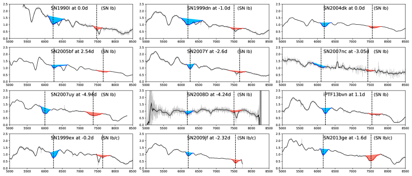
Figure 2: This figure shows all of the 9 published SN Ib and 3 SN Ib/c spectra around their maximum light. In each subplot, the silver, black, red, and blue solid line, as well as the colored filled region and black vertical dashed lines are the same as described in Figure 1. It is clear that compared with the SN Ia spectra in Figure 1, SN Ib peak spectra show relatively shallow $\lambda$6150 Å and O I absorption. The $\lambda$6150 Å  line is often blended with the He I line at $\lambda$6678 Å , which sometimes complicates our measurement of the $\lambda$6150 Å line depth. Name, type and phase information of each spectrum could be found on each subplot.

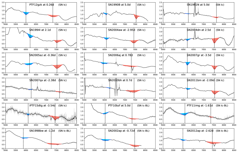
Figure 3: This figure shows all of the 13 published SN Ic and 5 SN Ic-BL spectra around their maximum light. In each subplot, the silver, black, red, and blue solid line, as well as the shading and black vertical dashed lines are the same as described in Figure 1. Note that settings the SN1998bw and PTF10bzf blue endpoints of the $\lambda$6150 Å line is tricky, making the analysis of these two object less reliable. Therefore we only report them for completeness. Compared with SN Ib spectra in Figure 2, we can find that SNe Ic have a relatively strong O I absorption, while their $\lambda$6150 Å  line depths are still much shallower than those of SN Ia presented in Figure 1. Name, type and phase information of each spectrum could be found on each subplot.

3 Analysis

3.1 Line Depth Measurement Method

In this section we describe our spectroscopic analysis method. Since we want to measure the line depth of the absorption regions around $\lambda$6150Å and $\lambda$7500Å relative to the pseudo-continuum, we adopt the line-depth technique presented in Silverman et al. (2012a) which was initially developed to measure the absorption region features of the BSNIP SN Ia sample. We will describe the technical details, including our improvement of their method in the following paragraphs. We then show a comparison between the Silverman et al. (2012a) and our measurement on BSNIP SNe Ia Si II and O I absorption line depths.

3.1.1 Initial Processing

For each of the spectra we listed in Table 1 and Table 3, we correct the wavelength to rest-frame using the host-galaxy redshifts presented in Table 1 and Table 2. Since interstellar reddening does not affect absorption line depth, we did not correct this effect.

Due to the high expansion velocity of the ejecta, the typical spectrum of a SN should not contain narrow absorption features. Therefore, it is reasonable to smooth the spectra and only retain broad spectral features for analysis. Each spectrum is smoothed using a Savitzky-Golay smoothing filter (Savitzky & Golay, 1964). The window size (frame length) and polynomial order for each spectrum is decided by its average wavelength interval, which is:

$$w=2\times\textrm{int}(\frac{50}{{\rm\Delta}\lambda})+1$$ (1)

$$o=\textrm{max}(3,\frac{w-1}{2})$$ (2)

where $w$ is the window size, $o$ is the polynomial order and ${\rm\Delta}\lambda$ is the average wavelength interval (in Å). By smoothing the spectra, we can effectively remove small scale abnormal flux values which could be due to cosmic rays, galactic or other possible contamination. The filtering process could help us deal with low SNR spectra rather than drop them.

3.1.2 Pseudo-Continuum and Line Depth

One of the most difficult steps in analyzing SN spectra is determining pseudo-continua for the absorption lines. Though the local minimum for the absorption is easy to determine both by eye and by machine, it is difficult to define the endpoints of an absorption line due to several reasons. As a result of the ejecta high expansion velocity, the absorption lines in SN spectra are quite broad, and absorptions due to different transitions can blend together (for example, Si II $\lambda$6355Å may blend with He I $\lambda$6678Å, which is common in SN Ib spectra). Furthermore, especially for SNe Ic-BL, the flux blueward of the Si II $\lambda$6355Å absorption often does not reach a peak before blending with the absorption around $\lambda$5000Å (for example, see SN1998ew’s spectrum in Figure 3). A similiar problem sometimes affectes O I $\lambda$7774Å because the continuum could have a sharp slope. All these effects make absorption line endpoints hard to determine.

In order to determine the range of the absorption regions around $\lambda$6150Å and O I $\lambda$7774Å, we decided to determine the endpoints manually. Though this method could introduce human error and some subjective bias in the endpoint definition, if the measurements are conducted by only one person during a short period, the human error will mainly result in a systematic shift and the fluctuation between measurements of different spectra will be relatively small. Besides, we can also examine our measurements by comparing our line depth results with Silverman et al. (2012a). We will present the result of this comparison at the end of this section.

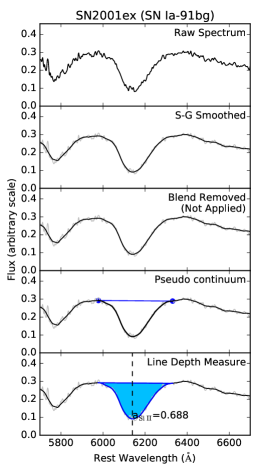
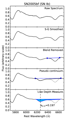
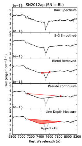
Figure 4: This figure shows the regular procedure of measuring an absorption line depth, including raw spectra, Savitzky-Golay smoothing, blend removal, pseudo-continuum determination and line depth measure (from top to bottom). Three example presented here are the SN2001ex Si II $\lambda$6355Å absorption, the SN2005bf absorption around $\lambda$6200Å (blended with He I $\lambda$6678Å; this absorption may not be due to Si II) and the SN2012ap O I $\lambda$7774Å absorption (heavily affected by the Fraunhofer A band around $\lambda$7594Å). Here “raw spectrum” means the original spectrum we adopted to analyze, which has been well-reduced. In order to show every change we made to the raw spectra, we plot every previous step result as silver line on the background.

In this work, the determination of the two absorption line endpoints of 181 Type I SNe are done by Fengwu Sun individually. For most cases, these endpoints present the closest peak (both blueward and redward) to the local minimum for the corresponding spectral feature, while for the situation that a nearby peak is quite far from the local minimum, we will choose the point where the spectral slope gets flat. If the absorption line is heavily blended with other lines, including other transitions in the SN photosphere, galactic emission lines, or even telluric lines, we will firstly remove this contaminating line with a linear sub-pseudo-continuum (simply replace the spectral feature with a line segment whose endpoints are the start and end points of this feature; Figure 4) and then determine the endpoints by the method we mentioned above. Under this de-blending condition, the endpoints for the absorption line may not be the intrinsic ones any longer (e.g. SN2005bf in Figure 4). Since we only care about the depth rather than the width, this de-blending trick will not bring negative effects to our measurements. In this way, line depth measurements are superior to (less sensitive than) pseudo-equivalent widths (pEWs).

Once the absorption line endpoints are determined, the pseudo-continua are calculated as a linear function with the two endpoints. If the spectrum is still not smooth within the corresponding wavelength range, we will fit this part of the spectrum using a polynomial model with a degree of 9. This step can enhance the precision of line depth measurements when the bottom of an absorption line is slightly fluctuating.

After finishing all the steps we mentioned above, We calculate the line depth of each absorption. The line depth ($a$) is defined as:

$$a={\rm max}\big{(}1-\frac{F_{\lambda}}{F_{\lambda,c}}\big{)}$$ (3)

Where $F_{\lambda,c}$ is the flux value of the pseudo-continuum, and $F_{\lambda}$ is the flux value of the spectrum after modification. Both $F_{\lambda,c}$ and $F_{\lambda}$ are functions of wavelength, and the line depth, i.e. the maximum for $1-{F_{\lambda}}/{F_{\lambda,c}}$ could always be found in a given wavelength range. We present three detailed examples of the line depth measurement procedure in Figure 4.

Table 4: Summary of abnormal discrepancies in BSNIP SN Ia Line Depth Measurements

SN Name	Absorption	Line Depth in	Line Depth	SN Name	Absorption	Line Depth in	Line Depth
	Line	Silverman et al. (2012a)	in this paper		Line	Silverman et al. (2012a)	in this paper
SN2000cp	O I	0.749	0.287	SN2001br	Si II	0.784	0.457
SN2001ex	O I	0.963	0.711	SN2001ex	Si II	0.813	0.688
SN2008s1	O I	0.598	0.406	SN2002aw	Si II	0.655	0.452
SN2000dn	Si II	0.762	0.659	SN2002de	Si II	0.779	0.530

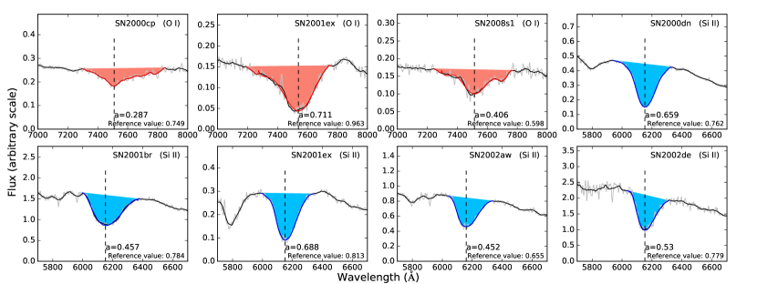
Figure 5: This figure shows all the 8 absorption lines whose depths are abnormally discrepant from the reference values. The silver, black, red, and blue solid line, as well as the colored filled region and black vertical dashed line are the same as described in Figure 1. Spectra are shifted such that the location of the Si II $\lambda$6355Å maximum line depth is at 6150 Å. Object name, line depth measurement result and reference value for each spectra are annotated on each subplot. By presenting this plot, we intend to demonstrate that our manual measurements are reasonable and convincing, in the cases that they differ from Silverman et al. (2012a) results.

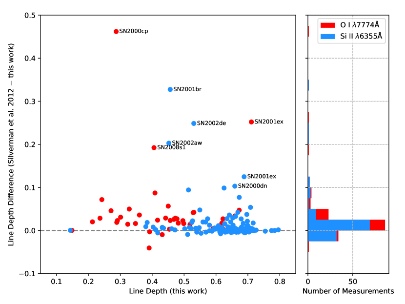
Figure 6: Left: Scatter plot of line depth measurement differences between this paper and Silverman et al. (2012a), where blue and red dots represent Si II $\lambda$6355Å and O I $\lambda$7774Å absorption line measurements respectively. For those objects whose differences are greater than 0.1, we also annotate their name on the plot.  Right: A histogram of line depth measurement differences between the two works. The size of the bins along the vertical axis is 0.025. Data in each bin are stacked together.

3.2 Examination

In order to assess the accuracy of our line depth result, we compare our measurements of BSNIP SNe Ia with Silverman et al. (2012a). 119 Si II $\lambda$6355Å and 40 O I $\lambda$7774Å line depth measurements among all our 146 SN Ia spectra have counterparts in Silverman et al. (2012a). Therefore, we plot a scatter diagram to observe the consistency between the two measurements (Figure 6, left panel). We also calculate the difference between the two independent measurements of each absorption line. A histogram of line depth measurement differences for Si II $\lambda$6355Å and O I $\lambda$7774Å is shown in the right panel of Figure 6.

Our interactive line depth measurement results are overall lower than Silverman et al. (2012a), however the mean value of the differences ($-0.024$) is small ($\sim$4% of the average line depth). Among all these 159 measurements, 144 (90.6%) are within 0.05 and 120 (75.5%) are within 0.025 of the Silverman et al. (2012a) results. Only 8 (5.0%) of these discrepancies are larger than 0.1 and these values are large enough to attract our attention. In Table 4 we list all these 8 abnormal measurement discrepancies. We also plot their spectra to demonstrate the validity of our measurements (see Figure 5). Inspection does not show any reason to suspect our result.

Alternatively, performing blind repeat measurements on both copies of the same spectra and other peak spectra of the same object taken a few days apart result in consistent measurements ($<10\%$ difference in values), which would not influence any of the results shown in the following section.

4 Result and Discussion

In this section we intend to present the line depth measurement results and analyze their statistical properties. Since a preliminary result of Type I SN quantitative classification criteria has been formulated in Gal-Yam (2016), here we will show an upgraded result with a larger sample size and more detailed subclass information.

4.1 Line Depth Measurement Results and Statistical Analysis

In Table 5 we present part of the line depth measurement results of 32 among all 181 Type I SN spectra, including 6 normal SNe Ia, 3 Ia-2002cx, 1 Ia-1991T, 4 Ia-1991bg, 4 Ia-1999aa, 1 Ia-pec, 3 regular SNe Ib, 4 SNe Ib/c, 4 regular SNe Ic and 2 Ic-BL (the full set of measurement results is available online). In addition to the results of the $\lambda 6150$Å and O I $\lambda$7774Å  line depths, we also calculate their ratio which would be used for analysis in the following paragraphs.

Table 5: Summary of Line Depth Measurement Result

SN Name	Type	$\lambda 6150$Å	O I $\lambda$7774Å	Line Depth	SN Name	Type	$\lambda 6150$Å	O I $\lambda$7774Å	Line Depth
		Depth	Depth	Ratio			Depth	Depth	Ratio
SN1989M	SN Ia	0.703	0.264	2.67	SN1994D	SN Ia	0.553	0.218	2.539
SN1994S	SN Ia	0.615	0.305	2.015	SN1995D	SN Ia	0.597	0.36	1.657
SN1999gd	SN Ia	0.687	0.271	2.535	SN1999gh	SN Ia	0.711	0.417	1.706
…	…	…	…	…	…	…	…	…	…
SN2003gq	SN Ia-02cx	0.165	0.275	0.6	SN2005hk	SN Ia-02cx	0.187	0.246	0.759
SN2008A	SN Ia-02cx	0.199	0.27	0.738	SN1997br	SN Ia-91T	0.144	0.153	0.94
SN1991bg	SN Ia-91bg	0.58	0.622	0.932	SN1999da	SN Ia-91bg	0.648	0.673	0.963
SN2001ex	SN Ia-91bg	0.688	0.711	0.968	SN2002cf	SN Ia-91bg	0.647	0.622	1.04
…	…	…	…	…	…	…	…	…	…
SN1998es	SN Ia-99aa	0.432	0.279	1.546	SN1999aa	SN Ia-99aa	0.432	0.259	1.668
SN1999dq	SN Ia-99aa	0.522	0.321	1.63	SN2001eh	SN Ia-99aa	0.527	0.263	2.005
…	…	…	…	…	…	…	…	…	…
SN2000cx	SN Ia-pec	0.384	0.199	1.932	SN1990I	SN Ib	0.346	0.238	1.456
SN1999dn	SN Ib	0.311	0.15	2.074	SN2004dk	SN Ib	0.268	0.148	1.814
…	…	…	…	…	…	…	…	…	…
PTF12hvv	SN Ib/c	0.202	0.479	0.421	SN1999ex	SN Ib/c	0.366	0.193	1.899
SN2009jf	SN Ib/c	0.224	0.4	0.559	SN2013ge	SN Ib/c	0.316	0.438	0.721
SN1991N	SN Ic	0.038	0.167	0.23	SN1994I	SN Ic	0.241	0.311	0.775
SN2002ap	SN Ic	0.134	0.454	0.295	SN2004aw	SN Ic	0.173	0.359	0.481
…	…	…	…	…	…	…	…	…	…
PTF11img	SN Ic-BL	0.193	0.103	1.872	SN2012ap	SN Ic-BL	0.119	0.25	0.477
…	…	…	…	…	…	…	…	…	…

• The table is abridged. The full table is available online.

• “Line Depth Ratio” here means the ratio of $\lambda 6150$Å depth to the O I $\lambda$7774Å depth, i.e. $a{\rm(\lambda 6150\AA)}/a{\rm(O\ I\ \lambda 7774\AA)}$

4.1.1 Statistics of SNe Ia Line Depth Properties

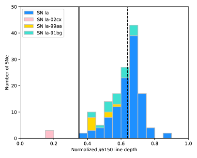
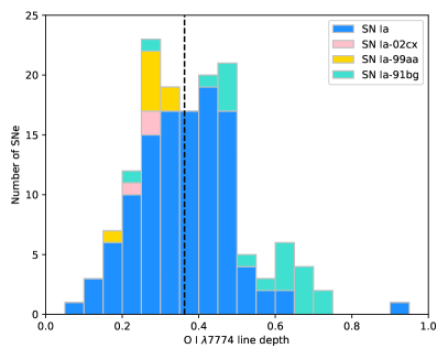
Figure 7: Left: Histogram of SNe Ia Si II $\lambda$6355Å line depth distribution. The black vertical solid line represents $a{\rm(\lambda 6150\AA)}=0.35$, while the dashed line represent the average for normal SNe Ia (blue bars) Si II $\lambda$6355Å line depth (0.638). Right: Histogram of the SN Ia O I $\lambda$7774Å line depth distribution. The dashed line represents the average for normal SN Ia (blue bars) O I $\lambda$7774Å line depth (0.363). Data in each bin are stacked together.

In order to study the line depth distribution properties of SNe Ia in our sample, we plot two histograms of SN Ia Si II $\lambda$6355Å and O I $\lambda$7774Å line depth distributions respectively in the left and right panel of Figure 7. Since we have only a single example of the 1991T-like subclass (SN1997br) and one Ia-pec (SN2000cx), these are excluded from this analysis.

From the left plot in Figure 7, we can see that 141 of 144 (97.9%) Type Ia SNe show a prominent Si II $\lambda$6355Å absorption with $a{\rm(\lambda 6150\AA)}>0.35$, except for the 3 SNe Ia-2002cx objects. The mean value for normal SNe Ia Si II $\lambda$6355Å depth is 0.638, represented by the dashed vertical line on the plot, with a standard deviation of 0.089. Generally, peculiar SNe Ia have shallower Si II $\lambda$6355Å lines than normal ones. SNe Ia-1991bg and Ia-1999aa are mostly located on the left of the dashed vertical line, while Ia-2002cx objects Si II $\lambda$6355Å depths are even less than 0.2. The single 1991T-like object also lies below $a{\rm(\lambda 6150\AA)}<0.35$, while SN2000cx is not an outlier ($a{\rm(\lambda 6150\AA)}=0.384$).

In the right panel of Figure 7, we can find SNe Ia in almost every bin of the O I $\lambda$7774Å line depth from 0.05 to 0.75. This phenomenon may indicate a diversity of O I optical depths in SN Ia photospheres. The dashed vertical line represents the mean value for normal SNe Ia O I $\lambda$7774Å line depth (0.363). However, it is obvious that the Ia-1991bg and Ia-1999aa object distributions are separated in this figure. The majority of SNe Ia-1991bg are located on the right of the dashed line, except for two outliers (SN2006ke and SN2008bt), indicating a larger O I $\lambda$7774Å line depth (mean: 0.551), while all the SNe Ia-1991aa are on the left (mean: 0.270). This could be related to the temperature sequence proposed by Nugent et al. (1995) extending from hot 1991T-like events to cool SNe Ia-1991bg. Three SNe Ia-2002cx also show shallow O I $\lambda$7774Å line depth ($a{\rm(O\ I\ \lambda 7774\AA)}<0.3$).

4.1.2 Statistics of SN Ib and Ic Line Depth Properties

Due to the low fraction of SNe Ib and Ic events among all Type I SNe, it is hard to obtain a large sample of SNe Ib&c peak spectra to analyze. Therefore, the statistical work we carry out will be relatively limited. However, it is still feasible to find some distinction between SNe Ib and Ic based on their line depth features.

In the left panel of Figure 8 we present the histogram of SN Ib and Ic $\lambda$6150Å line depth distribution. Except for a SN Ib outlier (PTF10feq) and a SN Ib/c outlier (SN1999ex), all of the objects in this plot are located on the left of the vertical solid black line at $a{\rm(\lambda 6150\AA)}=0.35$, which is also the left boundary of normal SNe Ia we discussed above. SNe Ib $\lambda$6150Å line depths are overall slightly larger than regular SNe Ic with significant overlap. The distribution range of SNe Ic-BL $\lambda$6150Å line depth is consistent with that of regular SNe Ic.

The histogram in the middle panel of Figure 8 shows the SN Ib and Ic O I $\lambda$7774Å line depth distributions. It is obvious in this subplot that SNe Ib show a generally shallower O I $\lambda$7774Å absorption than regular SNe Ic. The phenomenon we revealed here is in accord with several previous studies (for example, Matheson et al., 2001; Liu et al., 2016, and Fremling et al., in preparation). SNe Ic-BL O I $\lambda$7774Å line depths are somewhat lower than regular SNe Ic, i.e. closer to SNe Ib.

Since a small number of SNe Ib and regular SNe Ic are mixed in the central subplot, to distinguish them from each other, we adopt the line depth ratio of $\lambda$6150Å to $\lambda$7774Å, i.e. $a{\rm(\lambda 6150\AA)}/a{\rm(O\ I\ \lambda 7774\AA)}$, as another index. The right panel of Figure 8 shows the histogram of SN Ib and Ic line depth ratio distribution. From this subplot we can find that SNe Ib and regular SNe Ic are separated almost perfectly on the two sides of the vertical solid line at $a{\rm(\lambda 6150\AA)}/a{\rm(O\ I\ \lambda 7774\AA)}=1$, except for a SN Ic outlier, namely PTF12gzk. The line depth ratio of this object is only slightly above 1 (1.025), which is less than all the SNe Ib we analyze in this work. This result demonstrates that the line depth ratio could be used as a powerful index to distinguish the two types of SNe, though this index may not work well for SNe Ic-BL. Since Ic-BL can be easily distinguished from regular SNe Ib&c by their extreme expansion velocities, leading to prominent line widths in their spectra, this is not a major shortcoming of the method.

4.2 Quantitive Classification Criteria of Type I SNe

Based on the line depth measurements and the statistical analysis reported above, here we intend to present quantitive classification criteria for Type I SNe.

We have shown that all the regular SNe Ia, Ia-1991bg and Ia-1999aa events show prominent absorptions around $\lambda$6150Å whose depths are larger than 0.35, while SNe Ib and Ic $\lambda$6150Å depths are below this threshold. Therefore, it encourages us to adopt $a{\rm(\lambda 6150\AA)}$ as the first index to distinguish SNe Ia from regular SNe Ib and Ic. To show the distinction in OI $\lambda$7774Å line depth between SNe Ib and SNe Ic clearly, we decide to use the line depth ratio of $\lambda$6150Å to OI $\lambda$7774Å as the second index (Figure 8). We introduce the following set of quantitative classification criteria for the majority of Type I SNe as formulae:

1. SNe Ia (including normal Ia, Ia-1991bg and Ia-1999aa):

$$a{\rm(\lambda 6150\AA)}>0.35$$ (4)

2. SNe Ib:

$$a{\rm(\lambda 6150\AA)} <0.35;$$ (5)

$$a{\rm(\lambda 6150\AA)} /a{\rm(O\ I\ \lambda 7774\AA)}>1$$

3. SNe Ic (except for Ic-BL):

$$a{\rm(\lambda 6150\AA)} <0.35;$$ (6)

$$a{\rm(\lambda 6150\AA)} /a{\rm(O\ I\ \lambda 7774\AA)}<1$$

To show these criteria schematically, we plot a scatter diagram (Figure 9) to show all the 181 Type I SNe distribution of $\lambda$6150Å line depth and line depth ratio of $\lambda$6150Å to OI $\lambda$7774Å. From the figure we can see that all the normal SNe Ia, SNe Ia-1991bg and SNe Ia-1999aa are located on the right of vertical black dashed line at $a{\rm(\lambda 6150\AA)}=0.35$. SNe Ib mainly lie in the upper-left part of the diagram, except for a narrow outlier PTF10feq ($a{\rm(\lambda 6150\AA)}=0.353$). Regular SNe Ic are situated in the bottom left corner with $a{\rm(\lambda 6150\AA)}<0.35$ but $a{\rm(\lambda 6150\AA)}/a{\rm(O\ I\ \lambda 7774\AA)}<1$ except for PTF12gzk. Since PTF12gzk is reported to show high ejecta expansion velocities in peak spectra (e.g. Ben-Ami et al., 2012; Modjaz et al., 2016) resembling SN Ic-BL, its spectral line depth properties may have slight differences from regular SNe Ic. SNe Ia-2002cx objects locate in the same region as regular SNe Ic, while SNe Ic-BL seem to show up irregularly on the left of the vertical black dashed line. A single Ia-91T event is also an outlier.

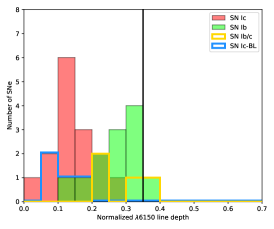
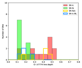
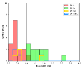
Figure 8: Left: Histogram of SNe Ib&c’s $\lambda$6150Å line depth distribution. The vertical solid black line represents $a{\rm(\lambda 6150\AA)}=0.35$, which is the left boundary of normal SNe Ia’s $\lambda$6150Å line depth.  Middle: Histogram of SNe Ib&c’s O I $\lambda$7774Å line depth.  Right: Histogram of SNe Ib&c’s line depth ratio of $\lambda$6150Å to $\lambda$7774Å . The vertical solid black line represents $a{\rm(\lambda 6150\AA)}/a{\rm(O\ I\ \lambda 7774\AA)}=1$, which is the boundary shared by regular SNe Ib and regular SNe Ic.

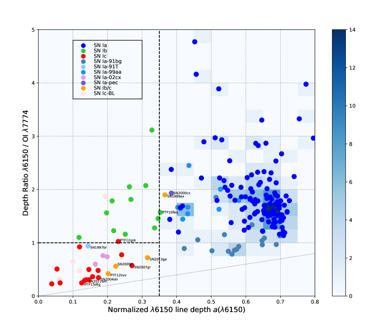
Figure 9: $\lambda$6150Å line depth versus line depth ratio of $\lambda$6150Å to OI $\lambda$7774Å of 181 Type I SNe. From this plot we can see the majority of SNe Ia (various kinds of blue dots; representing normal SNe Ia, Ia-1991bg, Ia-1999aa respectively) are located on the right of the vertical dashed line at $a{\rm(\lambda 6150\AA)}=0.35$, while regular SNe Ib (green dots) are on the upper-left part of the plot. Regular SNe Ic (red dots) as well as Ia-2002cx objects (violet dots) show a relatively shallower $\lambda$6150Å than normal SNe Ia but deeper OI $\lambda$7774Å absorption, so they are co-located with SNe Ic in the lower-left corner. All the names of SNe Ib/c (golden dots), the Ib outlier (PTF10feq), Ia-1991T (SN1997br as the light skyblue dot), Ia-pec (SN2000cx as the purple dot) as well as several SNe Ic are annotated on the plot. The background of the plot is a density map for normal SNe Ia, Ia-1991bg and Ia-1999aa, with the relevant color bar on the right.

4.3 Application and Discussion

The era of rapid development of observational techniques and instruments and international cooperation results in many SN discoveries, as well as many novel and strange SN subclasses. Among Type I SNe, the intermediate subtype between SN Ib and Ic, namely SN Ib/c, attracts our attention.

It is commonly reckoned that both SNe Ib and Ic originate from core collapse of massive stars that were stripped of their outermost hydrogen envelopes. For most conditions, SNe Ib are distinctive from SNe Ic due to helium features in their spectra around maximum light. However, the discovery of Type I SNe with transitional spectroscopic features between Type Ib and Ic SNe (e.g. SN1999ex, Hamuy et al., 2002; Stritzinger et al., 2002) indicates the difficulties of distinguishing these two types clearly and accurately.

Since the basic purpose of SN classification is to differentiate these events to several groups by their shared characters and distinctive features, we prefer to give a clear identifications to intermediate or unclear SNe Ib/c rather than leave them under an umbrella group. As we have already introduced a set of quantitative classification criteria for Type I SNe, it would be a feasible application and examination of our criteria to give clear identifications to these so-called SNe Ib/c.

Among our 4 SNe Ib/c objects, 3 (PTF12hvv, SN2009jf, SN2013ge) are located in the region of regular SNe Ic. PTF12hvv does not show conspicuous helium absorption in its optical spectrum, therefore it could be reclassified as a Type Ic SN. Similarly, SN2013ge (Drout et al., 2016) and SN 2009jf (Valenti et al., 2011) also show weak helium features, especially at both $\lambda$6678Å and $\lambda$7065Å , resembling SNe Ic.

Another SN Ib/c in our sample, SN1999ex, is located beyond but quite close to the right boundary of the SNe Ib region, with $a{\rm(\lambda 6150\AA)}=0.366$, which is quite similar to PTF10feq. With the notable He I $\lambda\lambda\lambda$5876Å 6678Å 7065Å features in its peak spectra, we have reason to believe this object can be reclassified as a Type Ib SN.

From all above we can carefully draw a conclusion that the majority of Type I SNe could be quantitatively classified according to their peak spectra. By measuring the line depth of $\lambda$6150Å and OI $\lambda$7774Å absorption around maximum light, we can simply give their location on the diagram and get their classification, with the only exception being the peculiar Ia-2002cx, Ic-BL and possibly Ia-91T subtypes. Meanwhile, there is no more need to identify Helium feature in their spectra to give an exact classification of Type I CCSNe, which may help to enhance the accuracy of determining a Type Ib or Ic classification.

Though a more detailed classification of a Type I SN may benefit from comparison and matching between the candidate spectrum and some well-calibrated template, or even better, a spectroscopic model (e.g. Hachinger et al., 2012), this simple and interactive line-depth classification method may give a quantitative way to classify these SNe, and thus could play an important role in the rapidly developing era of time-domain astronomy. Meanwhile, the physical implication of $a{\rm(\lambda 6150\AA)}/a{\rm(O\ I\ \lambda 7774\AA)}$ we introduced is not clear. This would be a good and natural question to target with physical models.

5 Summary

We have carried out a set of interactive $\lambda$6150Å and O I $\lambda$7774Å absorption line depth measurements on 181 Type I SN peak spectra. The Type I SN sample in this paper includes 146 SNe Ia (consisting of 133 normal Ia, 1 Ia-1991T, 21 Ia-1991bg, 8 Ia-1999aa and 3 Ia-2002cx), 12 SNe Ib, 19 SNe Ic (including 5 SNe Ic-BL) and 4 intermediate SN Ib/c. All the SN Ia objects we analyze here are from the low-redshift ($z<0.1$) BSNIP sample, while the SNe Ib and Ic we study here are acquired from WISeREP, originally from various publications, including 6 unpublished PTF and iPTF CCSNe. All the spectra are taken within 5 days of the SN maximum dates. For SNe Ia the dates of maximum are defined in B-band while V-band or g-band is typically used for SNe Ib and Ic, due to previous studies biases. We found that the majority of Type Ia SNe (excluding Ia-2002cx) show prominent $\lambda$6150Å absorption with depths greater than 0.35, while SNe Ib and Ic do not exceed this threshold. SNe Ib generally show a shallower O I $\lambda$7774Å absorption than regular SNe Ic, resulting in a line depth ratio of $\lambda$6150Å to O I $\lambda$7774Å greater than 1. This value is below 1 for the regular SNe Ic in our dataset. Therefore we generalize a set of quantitative classification criteria for Type I SNe. These criteria are based on line depth measurements of $\lambda$6150Å and O I $\lambda$7774Å absorption regions in SN peak spectra and can distinguish all major classes of Type I SNe, except for peculiar SNe Ia-2002cx and Ic-BL events. We apply this differentiating method to 4 transitional or unclear SNe Ib/c spectra. We find the classification results we derive are in high consistency with some previous classifications by identifying helium features in SN spectra. The physical meaning of the line depth ratio of $\lambda$6150Å to O I $\lambda$7774Å remains in need of an explanation.

References

- Aldering et al. (2005) Aldering, G., Lee, B. C., Loken, S., et al. 2005, The Astronomer’s Telegram, 451
- Astropy Collaboration et al. (2013) Astropy Collaboration, Robitaille, T. P., Tollerud, E. J., et al. 2013, A&A, 558, A33
- Barbon et al. (1999) Barbon, R., Buondí, V., Cappellaro, E., & Turatto, M. 1999, A&AS, 139, 531
- Bassett et al. (2007) Bassett, B., Becker, A., Bizyaev, D., et al. 2007, Central Bureau Electronic Telegrams, 1104
- Ben-Ami et al. (2012) Ben-Ami, S., Gal-Yam, A., Filippenko, A. V., et al. 2012, ApJ, 760, L33
- Benetti et al. (2011) Benetti, S., Turatto, M., Valenti, S., et al. 2011, MNRAS, 411, 2726
- Bianco et al. (2014) Bianco, F. B., Modjaz, M., Hicken, M., et al. 2014, ApJS, 213, 19
- Blondin & Calkins (2008) Blondin, S., & Calkins, M. 2008, Central Bureau Electronic Telegrams, 1191
- Blondin et al. (2012) Blondin, S., Matheson, T., Kirshner, R. P., et al. 2012, AJ, 143, 126
- Bloom et al. (2012) Bloom, J. S., Kasen, D., Shen, K. J., et al. 2012, ApJ, 744, L17
- Bufano et al. (2012) Bufano, F., Pian, E., Sollerman, J., et al. 2012, ApJ, 753, 67
- Cao et al. (2013) Cao, Y., Kasliwal, M. M., Arcavi, I., et al. 2013, ApJ, 775, L7
- Chornock et al. (2010) Chornock, R., Soderberg, A. M., Foley, R. J., et al. 2010, Central Bureau Electronic Telegrams, 2228
- Corsi et al. (2011) Corsi, A., Ofek, E. O., Frail, D. A., et al. 2011, ApJ, 741, 76
- Corsi et al. (2016) Corsi, A., Gal-Yam, A., Kulkarni, S. R., et al. 2016, ApJ, 830, 42
- Crockett et al. (2008) Crockett, R. M., Maund, J. R., Smartt, S. J., et al. 2008, ApJ, 672, L99
- Deng et al. (2000) Deng, J. S., Qiu, Y. L., Hu, J. Y., Hatano, K., & Branch, D. 2000, ApJ, 540, 452
- Drout et al. (2011) Drout, M. R., Soderberg, A. M., Gal-Yam, A., et al. 2011, ApJ, 741, 97
- Drout et al. (2016) Drout, M. R., Milisavljevic, D., Parrent, J., et al. 2016, ApJ, 821, 57
- Elias et al. (1985) Elias, J. H., Matthews, K., Neugebauer, G., & Persson, S. E. 1985, ApJ, 296, 379
- Elmhamdi et al. (2004) Elmhamdi, A., Danziger, I. J., Cappellaro, E., et al. 2004, A&A, 426, 963
- Filippenko (1997) Filippenko, A. V. 1997, ARA&A, 35, 309
- Filippenko et al. (2004a) Filippenko, A. V., Desroches, L., Ganeshalingam, M., Chornock, R., & Serduke, F. J. D. 2004a, IAU Circ., 8331
- Filippenko et al. (2004b) Filippenko, A. V., Ganeshalingam, M., Serduke, F. J. D., & Hoffman, J. L. 2004b, IAU Circ., 8404
- Filippenko & Korth (1991) Filippenko, A. V., & Korth, S. 1991, IAU Circ., 5234
- Filippenko et al. (1992) Filippenko, A. V., Richmond, M. W., Branch, D., et al. 1992, AJ, 104, 1543
- Folatelli et al. (2006) Folatelli, G., Contreras, C., Phillips, M. M., et al. 2006, ApJ, 641, 1039
- Folatelli et al. (2013) Folatelli, G., Morrell, N., Phillips, M. M., et al. 2013, ApJ, 773, 53
- Foley et al. (2003) Foley, R. J., Papenkova, M. S., Swift, B. J., et al. 2003, PASP, 115, 1220
- Foley et al. (2013) Foley, R. J., Challis, P. J., Chornock, R., et al. 2013, ApJ, 767, 57
- Fremling et al. (2014) Fremling, C., Sollerman, J., Taddia, F., et al. 2014, A&A, 565, A114
- Fremling et al. (2016) —. 2016, A&A, 593, A68
- Gal-Yam (2016) Gal-Yam, A. 2016, ArXiv e-prints, arXiv:1611.09353
- Gal-Yam et al. (2013) Gal-Yam, A., Mazzali, P. A., Manulis, I., & Bishop, D. 2013, PASP, 125, 749
- Gal-Yam et al. (2002) Gal-Yam, A., Ofek, E. O., & Shemmer, O. 2002, MNRAS, 332, L73
- Gal-Yam et al. (2001) Gal-Yam, A., Shemmer, O., & Dann, J. 2001, IAU Circ., 7622
- Galama et al. (1998) Galama, T. J., Vreeswijk, P. M., van Paradijs, J., et al. 1998, Nature, 395, 670
- Garavini et al. (2004) Garavini, G., Folatelli, G., Goobar, A., et al. 2004, AJ, 128, 387
- Graham & Li (2004) Graham, J., & Li, W. 2004, IAU Circ., 8381
- Hachinger et al. (2012) Hachinger, S., Mazzali, P. A., Taubenberger, S., et al. 2012, MNRAS, 422, 70
- Hamuy et al. (2002) Hamuy, M., Maza, J., Pinto, P. A., et al. 2002, AJ, 124, 417
- Harkness et al. (1987) Harkness, R. P., Wheeler, J. C., Margon, B., et al. 1987, ApJ, 317, 355
- Hunter et al. (2009) Hunter, D. J., Valenti, S., Kotak, R., et al. 2009, A&A, 508, 371
- Hunter (2007) Hunter, J. D. 2007, Computing In Science & Engineering, 9, 90
- Kasliwal et al. (2009) Kasliwal, M. M., Howell, J. L., Fox, D. B., Quimby, R., & Gal-Yam, A. 2009, Central Bureau Electronic Telegrams, 1955
- Kirshner (1994) Kirshner, R. 1994, IAU Circ., 5981
- Krisciunas et al. (2011) Krisciunas, K., Li, W., Matheson, T., et al. 2011, AJ, 142, 74
- Leloudas et al. (2009) Leloudas, G., Stritzinger, M. D., Sollerman, J., et al. 2009, A&A, 505, 265
- Li et al. (2001a) Li, W., Filippenko, A. V., Treffers, R. R., et al. 2001a, ApJ, 546, 734
- Li et al. (2001b) Li, W., Filippenko, A. V., Gates, E., et al. 2001b, PASP, 113, 1178
- Li et al. (2003) Li, W., Filippenko, A. V., Chornock, R., et al. 2003, PASP, 115, 453
- Liu et al. (2016) Liu, Y.-Q., Modjaz, M., Bianco, F. B., & Graur, O. 2016, ApJ, 827, 90
- Lyman et al. (2016) Lyman, J. D., Bersier, D., James, P. A., et al. 2016, MNRAS, 457, 328
- Malesani et al. (2009) Malesani, D., Fynbo, J. P. U., Hjorth, J., et al. 2009, ApJ, 692, L84
- Matheson et al. (2001) Matheson, T., Filippenko, A. V., Li, W., Leonard, D. C., & Shields, J. C. 2001, AJ, 121, 1648
- Mazzali et al. (2000) Mazzali, P. A., Iwamoto, K., & Nomoto, K. 2000, ApJ, 545, 407
- Mazzali et al. (2002) Mazzali, P. A., Deng, J., Maeda, K., et al. 2002, ApJ, 572, L61
- McCully et al. (2014) McCully, C., Jha, S. W., Foley, R. J., et al. 2014, ApJ, 786, 134
- Milisavljevic et al. (2013) Milisavljevic, D., Fesen, R., Pickering, T., et al. 2013, The Astronomer’s Telegram, 5142
- Milisavljevic et al. (2015) Milisavljevic, D., Margutti, R., Parrent, J. T., et al. 2015, ApJ, 799, 51
- Minkowski (1941) Minkowski, R. 1941, PASP, 53, 224
- Modjaz et al. (2008) Modjaz, M., Chornock, R., Foley, R. J., et al. 2008, Central Bureau Electronic Telegrams, 1222
- Modjaz et al. (2005) Modjaz, M., Kirshner, R., Challis, P., & Berlind, P. 2005, IAU Circ., 8522
- Modjaz et al. (2016) Modjaz, M., Liu, Y. Q., Bianco, F. B., & Graur, O. 2016, ApJ, 832, 108
- Modjaz et al. (2006) Modjaz, M., Stanek, K. Z., Garnavich, P. M., et al. 2006, ApJ, 645, L21
- Modjaz et al. (2009) Modjaz, M., Li, W., Butler, N., et al. 2009, ApJ, 702, 226
- Modjaz et al. (2014) Modjaz, M., Blondin, S., Kirshner, R. P., et al. 2014, AJ, 147, 99
- Morgan et al. (1943) Morgan, W. W., Keenan, P. C., & Kellman, E. 1943, An atlas of stellar spectra, with an outline of spectral classification
- Nugent et al. (1995) Nugent, P., Phillips, M., Baron, E., Branch, D., & Hauschildt, P. 1995, ApJ, 455, L147
- Nugent et al. (2011) Nugent, P. E., Sullivan, M., Cenko, S. B., et al. 2011, Nature, 480, 344
- Östman et al. (2011) Östman, L., Nordin, J., Goobar, A., et al. 2011, A&A, 526, A28
- Parrent et al. (2016) Parrent, J. T., Milisavljevic, D., Soderberg, A. M., & Parthasarathy, M. 2016, ApJ, 820, 75
- Phillips (1990) Phillips, M. M. 1990, IAU Circ., 5032
- Pian et al. (2006) Pian, E., Mazzali, P. A., Masetti, N., et al. 2006, Nature, 442, 1011
- Prentice et al. (2016) Prentice, S. J., Mazzali, P. A., Pian, E., et al. 2016, MNRAS, 458, 2973
- Quimby et al. (2005) Quimby, R., Hoeflich, P., Wheeler, J. C., et al. 2005, IAU Circ., 8504
- Rich et al. (2011) Rich, D., Brimacombe, J., Gall, E., et al. 2011, Central Bureau Electronic Telegrams, 2695
- Richmond et al. (1996) Richmond, M. W., van Dyk, S. D., Ho, W., et al. 1996, AJ, 111, 327
- Sahu et al. (2009) Sahu, D. K., Anupama, G. C., & Gurugubelli, U. K. 2009, Central Bureau Electronic Telegrams, 1955
- Sahu et al. (2011) Sahu, D. K., Gurugubelli, U. K., Anupama, G. C., & Nomoto, K. 2011, MNRAS, 413, 2583
- Savitzky & Golay (1964) Savitzky, A., & Golay, M. J. E. 1964, Analytical Chemistry, 36, 1627
- Silverman et al. (2012a) Silverman, J. M., Kong, J. J., & Filippenko, A. V. 2012a, MNRAS, 425, 1819
- Silverman et al. (2012b) Silverman, J. M., Foley, R. J., Filippenko, A. V., et al. 2012b, MNRAS, 425, 1789
- Silverman et al. (2013) Silverman, J. M., Vinko, J., Kasliwal, M. M., et al. 2013, MNRAS, 436, 1225
- Smartt (2009) Smartt, S. J. 2009, ARA&A, 47, 63
- Srivastav et al. (2014) Srivastav, S., Anupama, G. C., & Sahu, D. K. 2014, MNRAS, 445, 1932
- Stritzinger et al. (2002) Stritzinger, M., Hamuy, M., Suntzeff, N. B., et al. 2002, AJ, 124, 2100
- Stritzinger et al. (2009) Stritzinger, M., Mazzali, P., Phillips, M. M., et al. 2009, ApJ, 696, 713
- Stritzinger et al. (2011) Stritzinger, M. D., Phillips, M. M., Boldt, L. N., et al. 2011, AJ, 142, 156
- Taddia et al. (2015) Taddia, F., Sollerman, J., Leloudas, G., et al. 2015, A&A, 574, A60
- Taddia et al. (2016) Taddia, F., Fremling, C., Sollerman, J., et al. 2016, A&A, 592, A89
- Taubenberger et al. (2006) Taubenberger, S., Pastorello, A., Mazzali, P. A., et al. 2006, MNRAS, 371, 1459
- Valenti et al. (2008) Valenti, S., Elias-Rosa, N., Taubenberger, S., et al. 2008, ApJ, 673, L155
- Valenti et al. (2011) Valenti, S., Fraser, M., Benetti, S., et al. 2011, MNRAS, 416, 3138
- Valenti et al. (2012) Valenti, S., Taubenberger, S., Pastorello, A., et al. 2012, ApJ, 749, L28
- Van Der Walt et al. (2011) Van Der Walt, S., Colbert, S. C., & Varoquaux, G. 2011, Computing in Science & Engineering, 13, 22
- van Dyk (1992) van Dyk, S. D. 1992, AJ, 103, 1788
- van Dyk et al. (1993) van Dyk, S. D., Sramek, R. A., Weiler, K. W., & Panagia, N. 1993, ApJ, 409, 162
- Wheeler & Harkness (1990) Wheeler, J. C., & Harkness, R. P. 1990, Reports on Progress in Physics, 53, 1467
- Wheeler et al. (1995) Wheeler, J. C., Harkness, R. P., Khokhlov, A. M., & Hoeflich, P. 1995, Phys. Rep., 256, 211
- Wheeler & Levreault (1985) Wheeler, J. C., & Levreault, R. 1985, ApJ, 294, L17
- White et al. (2015) White, C. J., Kasliwal, M. M., Nugent, P. E., et al. 2015, ApJ, 799, 52
- Woosley & Bloom (2006) Woosley, S. E., & Bloom, J. S. 2006, ARA&A, 44, 507
- Xu et al. (2013) Xu, D., de Ugarte Postigo, A., Leloudas, G., et al. 2013, ApJ, 776, 98
- Yaron & Gal-Yam (2012) Yaron, O., & Gal-Yam, A. 2012, PASP, 124, 668