An Adaptive, Multivariate Partitioning Algorithm for Global Optimization of Nonconvex Programs

Abstract

In this work, we develop an adaptive, multivariate partitioning algorithm for solving nonconvex, Mixed-Integer Nonlinear Programs (MINLPs) with polynomial functions to global optimality. In particular, we present an iterative algorithm that exploits piecewise, convex relaxation approaches via disjunctive formulations to solve MINLPs that is different than conventional spatial branch-and-bound approaches. The algorithm partitions the domains of variables in an adaptive and non-uniform manner at every iteration to focus on productive areas of the search space. Furthermore, domain reduction techniques based on sequential, optimization-based bound-tightening and piecewise relaxation techniques, as a part of a presolve step, are integrated into the main algorithm. Finally, we demonstrate the effectiveness of the algorithm on well-known benchmark problems (including Pooling and Blending instances) from MINLPLib and compare our algorithm with state-of-the-art global optimization solvers. With our novel approach, we solve several large-scale instances, some of which are not solvable by state-of-the-art solvers. We also succeed in reducing the best known optimality gap for a hard, generalized pooling problem instance.

1 Introduction

Mixed-Integer Nonlinear Programs (MINLPs) are convex/non-convex, mathematical programs that include discrete variables and nonlinear terms in the objective function and/or constraints. In practice, non-convex MINLPs arise in many applications such as chemical engineering (synthesis of process and water networks) meyer2006global ; ryoo1995global , energy infrastructure networks hijazi2016 ; lu_optimal_tps2017 ; nagarajan2016optimal , and in molecular distance geometry problems liberti2008branch , to name a few. Given the importance of these problems, considerable research has been devoted to developing approaches for solving MINLPs, such as approaches implemented in such solvers as BARON sahinidis1996baron , Couenne belotti2009branching and SCIP achterberg2009scip . Within these approaches, two of the key features of successful methods include MINLP relaxations and search. For example, in a typical solver, non-convex terms are replaced with convex over- and under-estimators boukouvala2016global . The resulting convex optimization problem is a relaxation of the original MINLP and its solution is a bound to the optimal objective value of the MINLP. These relaxations are then used in conjunction with a search procedure, like spatial branch-and-bound (sBB), to explore the solution space of the MINLP and identify the global optimal solution.

Despite major developments related to these features and others, MINLPs still remain difficult to solve and global optimization solvers often struggle to find optimal solutions and at times, even a feasible solution. In many cases, the source of these struggles are weak relaxations of the MINLP and the impact weak relaxations on the size of the search space that is explored. To address these difficulties, in this paper we develop an approach for deriving better bounds through piecewise convex relaxations that are modeled as mixed-integer convex optimization problems. The piecewise convex relaxations are combined with additional algorithmic enhancements, a novel, adaptive domain partitioning scheme, and successive solves of mixed-integer problems (MIP), to produce a novel search procedure. This global optimization algorithm is tested extensively on MINLPs with polynomial constraints, including the well-known and hard Pooling and Blending instances kolodziej2013discretization and is compared with state-of-the-art global optimization approaches. In this paper, we focus on MINLPs with polynomial constraints, but the approach is fairly generic and can be generalized to other nonconvex functions. Finally, for ease of exposition, we assume the MINLPs are minimization problems throughout the rest of the paper.

We next discuss the key contributions we make in this paper. Our first contribution improves convex relaxations of polynomial functions. Here, we develop an approach based on piecewise convex relaxations. While such relaxations have been used to bound medium-sized MINLPs with bilinear functions castro2015tightening ; hasan2010piecewise ; karuppiah2006global ; kolodziej2013discretization ; bergamini2008improved , we generalize these approaches to arbitrary polynomial functions.

Our second contribution turns the derivation of these relaxations into a search procedure based on solving MIPs, i.e., a ‘MIP-based approach’ that is akin to the approach of ruiz2017global ; faria2012new . Most existing approaches rely on sBB. In a conventional sBB algorithm, branching occurs on the domain of one variable at a time. The branching generates two new problems (child nodes), each with a smaller domain than the parent problem (node) and potentially tighter relaxations. Whenever the best possible solution at a node is worse than the best known feasible solution, the node is pruned. sBB is typically combined with with enhancements such as cutting planes and domain reduction techniques to further improve the efficiency of the search sahinidis1996baron ; tawarmalani2005polyhedral . In contrast, our MIP-based approach solves a sequence of MIPs based on successively tighter piecewise convex relaxations that converges to the optimal solution.

Our third contribution is a sparse domain partitioning approach for piecewise convex relaxations. Most existing partitioning approaches rely on uniform partitioning, i.e., hasan2010piecewise . Unfortunately, uniform partitioning, when used in conjunction with a MIP-based approach can lead to MIPs with a large number of binary variables. Thus, uniform partitioning limits MIP based approaches to small- and medium-sized problems. This important issue has motivated the development of piecewise relaxation techniques where the number of binary variables increases logarithmically misener2011apogee ; Vielma2009 with the number of partitions and multiparametric disaggregation approaches castro2015normalized . In other work wicaksono2008piecewise , the authors present a non-uniform, bivariate partitioning approach that improves the relaxations but provide results for a single, simple benchmark problem. Reference teles2013univariate discusses a univariate parametrization method applied to medium-sized benchmarks. However, none of these approaches address the key limitation of uniform partitioning, partition density, i.e. these methods introduce partitions in unproductive areas of the variable domains. We address this limitation by introducing a novel approach that adaptively partitions the relaxations in regions of the search space that favor optimality. To the best of our knowledge, this is the first work in the literature that develops a complete MIP-based method for solving MINLPs to global optimality based on sparse domain partitioning schemes.

Our fourth (minor) contribution combines the adaptively partitioned piecewise relaxation approach with sequential, optimization-based bound-tightening (OBBT). OBBT is used as a presolve step in the overall global optimization algorithm. OBBT solves a sequence of convex minimization and maximization problems on the variables that appear in nonconvex terms. The solutions to these problems tighten domains of the variables and the associated relaxation to the nonconvex terms puranik2017domain ; belotti2012feasibility ; faria2011novel ; mouret2009tightening . Recent work has observed the effectiveness of applying OBBT in various applications coffrin2015strengthening ; fei2017acc ; nagarajan2017r2r . We adapt and extend this approach by solving convex MIPs in the OBBT procedure (existing approaches solve ordinary convex problems). Though this approach seems counter-intuitive, computational experiments indicate that the value of the strengthened bounds obtained by solving MIPs often outweigh the computational time required to solve them.

Finally, these four contributions are combined into a MIP-based global optimization algorithm which is referred to as the Adaptive, Multivariate Partitioning (AMP) algorithm. Given an MINLP, AMP first calculates a local solution to the MINLP, an initial lower bound, and tightened variable bounds (sequential OBBT) as a presolve step. The main loop of the AMP algorithm refines the partitions of the variable domain, computes improved lower bounds, and derives better local (upper bound) solutions. The variable domains are refined in a non-uniform and adaptive fashion. In particular, partitions are dynamically added around the optimal solution to the relaxed problem at each iteration of AMP. This loop iterates until the relative gap between the lower bound and the upper bound solution meets a user specified global optimality tolerance. The computation may also be interrupted early to provide a local optimal solution.

A preliminary version of this work nagarajan2016tightening was applied to hard, infrastructure network optimization problems fei2017acc ; LuPSCC2017 , which demonstrated the effectiveness of adaptive partitioning strategies. Given the efficacy of the proposed ideas, including various enhancements (not discussed in this paper), the algorithm’s implementation is also available as an open-source solver in Julia programming language bent2017polyhedral . The remainder of this paper is organized as follows: Section 2 discusses the required notation, problem set-up, and reviews standard convex relaxations. Section 3 discusses our Adaptive, Multivariate Partitioning Algorithm to solve MINLPs to global optimality with a few proofs of convergence guarantees. Section 4 illustrates the strength of the algorithms on benchmark MINLPs and Section 5 concludes the paper.

2 Definitions

Notation

Here, we use lower and upper case for vector and matrix entries, respectively. Bold font refers to the entire vector or matrix. With this notation, $||\bm{v}||_{\infty}$ defines the $\ell^{\infty}$ norm of vector $\bm{v}\in\mathbb{R}^{n}$. Given vectors $\bm{v}_{1}\in\mathbb{R}^{n}$ and $\bm{v}_{2}\in\mathbb{R}^{n}$, $\bm{v}_{1}\cdot\bm{v}_{2}=\sum_{i=1}^{n}{v_{1}}_{i}{v_{2}}_{i}$; $\bm{v}_{1}+\bm{v}_{2}$ implies element-wise sums; and $\frac{\bm{v}_{1}}{\alpha}$ denotes the element-wise ratio between entries of $\bm{v}_{1}$ and the scalar $\alpha$. Next, $z\in\mathbb{Z}$ represents an integer (variable/constant) and specifically $z\in\mathbb{B}$ represents a binary variable. Finally, we let $\bm{e}_{i}$ denote a unit vector whose $i$^th coordinate is one.

Problem

The problems considered in this paper are MINLPs with polynomials which have at least one feasible solution. The general form of the problem, denoted as $\bm{\mathcal{P}}$, is as follows:

$$\bm{\mathcal{P}}: \underset{\bm{x},\bm{y}}{\text{minimize}} f(\bm{x},\bm{y})$$

subject to $$\bm{g}(\bm{x},\bm{y})\leqslant 0,$$

$$\bm{h}(\bm{x},\bm{y})=0,$$

$$\bm{x}^{L}\leqslant\bm{x}\leqslant\bm{x}^{U},$$

$$\bm{y}\in\{0,1\}^{m}$$

where, $f:\mathbb{R}^{n}\times\mathbb{B}^{m}\rightarrow\mathbb{R}$, $g_{i}:\mathbb{R}^{n}\times\mathbb{B}^{m}\rightarrow\mathbb{R}\ \mathrm{for}\ i=1,\ldots,G$ and $h_{i}:\mathbb{R}^{n}\times\mathbb{B}^{m}\rightarrow\mathbb{R}\ \mathrm{for}\ i=1,\ldots,H$ are polynomials. For the sake of clarity, neglecting the binary variables in the functions, $f,\bm{g}$ or $\bm{h}$ can assume the following form:

$$\sum_{t\in T}a_{t}\prod_{k\in K_{t}}x^{\alpha_{k}}_{k}$$ (1)

where, $T$ is a set of terms in a polynomial, $K_{t}$ is a set of variables in term $t$, $a_{t}\in\mathbb{R}$ is a real coefficient and $\alpha_{k}$ is an exponent (integer) value. $\bm{x}$ and $\bm{y}$ are vectors of continuous variables with box constraints [$\bm{x}^{L},\bm{x}^{U}$] and binary variables, respectively. $\bm{x}$ and $\bm{y}$ have dimension $n$ and $m$, respectively. We use notation $\sigma$ to denote a solution to $\bm{\mathcal{P}}$, where $\sigma(\cdot)$ is the value of variable(s), $\cdot$, in $\sigma$ and $f(\sigma)$ is the objective value of $\sigma$. We note that $\bm{\mathcal{P}}$ is an NP-hard combinatorial problem. The construction of convex relaxations for each individual term in Eq. (1) plays a critical role in developing algorithms for solving $\bm{\mathcal{P}}$ to global optimality. In the following paragraphs, we discuss the relaxations used in this paper.

In this paper, we use relaxations for bilinear, multilinear and quadratic monomials. Note that, without loss of generality, any polynomial can be equivalently expressed using a combination of these monomials.

McCormick relaxation of a bilinear term

For $t\in T$, when $|K_{t}|\leqslant 2$ and $\alpha_{k}=1$, the McCormick relaxation mccormick1976computability is used. Given variables $x_{i}$ and $x_{j}$ that appear in $t$, McCormick relaxed the set

$$S_{B}=\left\{(x_{i},x_{j},\widehat{x_{ij}})\in[x_{i}^{L},x_{i}^{U}]\times[x_{j}^{L},x_{j}^{U}]\times\mathbb{R}\mid\widehat{x_{ij}}=x_{i}x_{j}\right\}$$

with the following four inequalities:

$$\widehat{x_{ij}} \geqslant x_{i}^{L}x_{j}+x_{j}^{L}x_{i}-x_{i}^{L}x_{j}^{L}$$ (2a)

$$\widehat{x_{ij}} \geqslant x_{i}^{U}x_{j}+x_{j}^{U}x_{i}-x_{i}^{U}x_{j}^{U}$$ (2b)

$$\widehat{x_{ij}} \leqslant x_{i}^{L}x_{j}+x_{j}^{U}x_{i}-x_{i}^{L}x_{j}^{U}$$ (2c)

$$\widehat{x_{ij}} \leqslant x_{i}^{U}x_{j}+x_{j}^{L}x_{i}-x_{i}^{U}x_{j}^{L}$$ (2d)

Let $\langle x_{i},x_{j}\rangle^{MC}\supset S_{B}$ represent the feasible region defined by (2). For a single bilinear term $x_{i}x_{j}$, the relaxations in (2) describe the convex hull of set $S_{B}$ al1983jointly .

Recursive McCormick relaxation of a multilinear term

For a general multilinear term ($|K_{t}|\geqslant 3$, $\alpha_{k}=1$), McCormick proposed a recursive approach to successively derive envelopes on bilinear combinations of the terms. The resulting relaxation has formed the basis for the relaxations used in the global optimization literature, including the implementations in BARON, Couenne and SCIP sahinidis1996baron ; belotti2009branching ; achterberg2009scip . More formally, the non-convex function given by $\prod_{k=1}^{|K_{t}|}x_{k}$ can be relaxed by introducing lifted variables $\widehat{x}_{1},\ldots,\widehat{x}_{|K_{t}|-1}$ such that $\widehat{x}_{1}=x_{1}x_{2}$ and $\widehat{x}_{i}=\widehat{x}_{i-1}x_{i+1}$ for every $i=2,\ldots,|K_{t}|-1$. Thus, the recursive McCormick envelopes of $\prod_{k=1}^{|K_{t}|}x_{k}$ are described by

$$\left\{(x_{1},x_{2},\widehat{x}_{1})\in[x_{1}^{L},x_{1}^{U}]\times[x_{2}^{L},x_{2}^{U}]\times[\widehat{x}_{1}^{L},\widehat{x}_{1}^{U}]\mid\widehat{x}_{1}=\langle x_{1},x_{2}\rangle^{MC}\right\},$$ (3a)

$$\left\{(\widehat{x}_{i-1},x_{i+1},\widehat{x}_{i})\in[\widehat{x}_{i-1}^{L},\widehat{x}_{i-1}^{U}]\times[x_{i+1}^{L},x_{i+1}^{U}]\times[\widehat{x}_{i}^{L},\widehat{x}_{i}^{U}]\mid\right.$$

$$\hskip 96.73918pt\left.\widehat{x}_{i}=\langle\widehat{x}_{i-1},x_{i+1}\rangle^{MC}\right\},\quad\forall i=2,\ldots,|K_{t}|-1.$$ (3b)

where, the bounds of $\widehat{x}_{i}$ variables are derived appropriately. By abuse of notation, (3) can be succinctly represented as

$$\left\langle\prod_{k=1}^{|K_{t}|}x_{k}\right\rangle^{MC}=\left\langle\left\langle\left\langle x_{1},x_{2}\right\rangle^{MC},\ldots,x_{|K_{t}|-1}\right\rangle^{MC},x_{|K_{t}|}\right\rangle^{MC}.$$

In general, the recursive McCormick envelopes described in (3) for a single multilinear term are not the tightest possible relaxation. The choice of the recursion order affects the tightness of the relaxation Speakman2017 ; cafieri2010convex . However, authors in ryoo2001analysis prove that (3) describes the convex hull when the bounds on the variables are in the set $[0,1]$. This result was generalized by luedtke2012some for variables with bounds that are either $[0,x^{U}_{i}]$ or [$-x^{U}_{i},x^{U}_{i}$] (symmetric about the origin). More generally, the convex hull of a multilinear term can be obtained by using an extreme point characterization by using exponential number of variables Rikun1997 . The computational tractability of using an extreme point characterization for piecewise relaxation of multilinear terms remains a subject of future work.

Piecewise McCormick relaxation of a bilinear term

In the presence of partitions on the variables involved in a multilinear term, the McCormick relaxations (applied on bilinear terms) can be tightened (see Figure 1[a]) by using a piecewise convex relaxation which uses one binary variable per variable partition. Given a bilinear term $x_{i}x_{j}$ and partition sets $\bm{\mathcal{I}}_{i}$ and $\bm{\mathcal{I}}_{j}$, binary variables $\widehat{\bm{y}}_{i}\in\{0,1\}^{|\bm{\mathcal{I}}_{i}|}$ and $\widehat{\bm{y}}_{j}\in\{0,1\}^{|\bm{\mathcal{I}}_{j}|}$ are used to denote these partitions. Each entry in $\bm{\mathcal{I}}_{i}$ is a pair of values, $\langle i,j\rangle$ that model the upper and lower bound of a variable in a partition. We refer to the collection of all partition sets with $\bm{\mathcal{I}}$. These binary variables are used to control the partitions that are active and the associated relaxation of the active partition. Formally, the piecewise McCormick constraints, denoted by $\widehat{x_{ij}}\in\langle x_{i},x_{j}\rangle^{MC(\bm{\mathcal{I}})}$, take the following form:

$$\widehat{x_{ij}}\geqslant(\bm{x}_{i}^{l}\cdot\widehat{\bm{y}}_{i})x_{j}+(\bm{x}_{j}^{l}\cdot\widehat{\bm{y}}_{j})x_{i}-(\bm{x}_{i}^{l}\cdot\widehat{\bm{y}}_{i})(\bm{x}_{j}^{l}\cdot\widehat{\bm{y}}_{j})$$ (4a)

$$\widehat{x_{ij}}\geqslant(\bm{x}_{i}^{u}\cdot\widehat{\bm{y}}_{i})x_{j}+(\bm{x}_{j}^{u}\cdot\widehat{\bm{y}}_{j})x_{i}-(\bm{x}_{i}^{u}\cdot\widehat{\bm{y}}_{i})(\bm{x}_{j}^{u}\cdot\widehat{\bm{y}}_{j})$$ (4b)

$$\widehat{x_{ij}}\leqslant(\bm{x}_{i}^{l}\cdot\widehat{\bm{y}}_{i})x_{j}+(\bm{x}_{j}^{u}\cdot\widehat{\bm{y}}_{j})x_{i}-(\bm{x}_{i}^{l}\cdot\widehat{\bm{y}}_{i})(\bm{x}_{j}^{u}\cdot\widehat{\bm{y}}_{j})$$ (4c)

$$\widehat{x_{ij}}\leqslant(\bm{x}_{i}^{u}\cdot\widehat{\bm{y}}_{i})x_{j}+(\bm{x}_{j}^{l}\cdot\widehat{\bm{y}}_{j})x_{i}-(\bm{x}_{i}^{u}\cdot\widehat{\bm{y}}_{i})(\bm{x}_{j}^{l}\cdot\widehat{\bm{y}}_{j})$$ (4d)

$$\widehat{\bm{y}}_{i}\cdot\bm{1}=1,\ \ \widehat{\bm{y}}_{j}\cdot\bm{1}=1$$ (4e)

$$\widehat{\bm{y}}_{i}\in\{0,1\}^{|\bm{\mathcal{I}}_{i}|},\quad\widehat{\bm{y}}_{j}\in\{0,1\}^{|\bm{\mathcal{I}}_{j}|}$$ (4f)

where, $(\bm{x}_{i}^{l},\bm{x}_{i}^{u})\in\bm{\mathcal{I}}_{i}$ are the vector form of the partition sets of $x_{i}$ ($\bm{\mathcal{I}}_{i}$) and $\bm{1}$ is a vector of ones of appropriate dimension. Also, $(\bm{x}_{i}^{l}\cdot\widehat{\bm{y}}_{i})(\bm{x}_{j}^{l}\cdot\widehat{\bm{y}}_{j})$ is rewritten as $\bm{x}_{i}^{l}(\widehat{\bm{y}}_{i}\widehat{\bm{y}}_{j}^{T})\bm{x}_{j}^{l}$, where $(\widehat{\bm{y}}_{i}\widehat{\bm{y}}_{j}^{T})$ is a matrix with binary product entries. Note that these binary products and the bilinear terms in $\widehat{\bm{y}}_{j}x_{i}$ and $\widehat{\bm{y}}_{i}x_{j}$ can be linearized exactly using standard McCormick relaxations nagarajan2018lego .

It is then straightforward to generalize piecewise McCormick relaxations to multilinear terms, and we use the following notation to denote these relaxations

$$\left\langle\prod_{k=1}^{|K_{t}|}x_{k}\right\rangle^{MC(\bm{\mathcal{I}})}=\left\langle\left\langle\left\langle x_{1},x_{2}\right\rangle^{MC(\bm{\mathcal{I}})},\ldots,x_{|K_{t}|-1}\right\rangle^{MC(\bm{\mathcal{I}})},x_{|K_{t}|}\right\rangle^{MC(\bm{\mathcal{I}})}.$$

We also note that the McCormick relaxation is a special case of the piecewise McCormick relaxation when $\bm{\mathcal{I}}_{i}=\{\langle x^{L}_{i},x^{U}_{i}\rangle\}$.

These relaxations can also be encoded using $\log(|\bm{\mathcal{I}}_{i}|)$ binary variables DAmbrosio2010 ; Li2013b ; Vielma2009 or variations of special order sets (SOS1, SOS2). For an ease of exposition, we do not present the details of the log-based formulation in this paper. However, later in the results section, we do compare the effectiveness of SOS1 formulations with respect to the linear representation of binary variables.

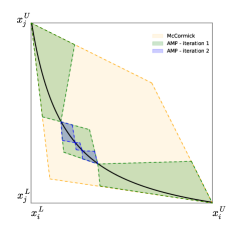
(a) Bilinear term $(x_{i}x_{j})$

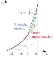
(b) Quadratic term $(x_{i}^{2})$

Figure 1: Piecewise relaxations (shaded) of bilinear and quadratic terms for a given set of partitions.

Piecewise relaxation of a quadratic term

Without loss of generality, assume a univariate monomial takes the form $x_{i}^{2}$. Though, we restrict our discussion to a univariate monomial, similar extensions hold true for a multivariate monomial by applying a sequence of relaxations on the respective univariate monomials. Given partitions in $\bm{\mathcal{I}}_{i}$, the piecewise, convex relaxation (see Figure 1[b]), denoted by $\widehat{x}_{i}\in\langle x_{i}\rangle^{MC_{q}(\bm{\mathcal{I}})}$, takes the form:

$$\widehat{x}_{i}\geqslant x_{i}^{2},$$ (5a)

$$\widehat{x}_{i}\leqslant\left((\bm{x}_{i}^{l}\cdot\widehat{\bm{y}}_{i})+(\bm{x}_{i}^{u}\cdot\widehat{\bm{y}}_{i})\right)x_{i}-(\bm{x}_{i}^{l}\cdot\widehat{\bm{y}}_{i})(\bm{x}_{i}^{u}\cdot\widehat{\bm{y}}_{i})$$ (5b)

$$\widehat{\bm{y}}_{i}\cdot\bm{1}=1$$ (5c)

$$\widehat{\bm{y}}_{i}\in\{0,1\}^{|\bm{\mathcal{I}}_{i}|}$$ (5d)

Once again, $(\bm{x}_{i}^{l}\cdot\widehat{\bm{y}}_{i})(\bm{x}_{i}^{u}\cdot\widehat{\bm{y}}_{i})$ is rewritten as $\bm{x}_{i}^{l}(\widehat{\bm{y}}_{i}\widehat{\bm{y}}_{i}^{T})\bm{x}_{i}^{u}$, where $\widehat{\bm{y}}_{i}\widehat{\bm{y}}_{i}^{T}$ is a symmetric matrix with binary product entries (squared binaries on diagonal). Hence, it is sufficient to linearize the entries of the upper triangular matrix with exact representations. We also note again that the unpartitioned relaxation is a special case where $\bm{\mathcal{I}}_{i}=\{\langle x^{L}_{i},x^{U}_{i}\rangle\}$.

Lemma 1.

$\langle x_{i}\rangle^{MC_{q}(\bm{\mathcal{I}})}\subset\langle x_{i},x_{i}\rangle^{MC(\bm{\mathcal{I}})}$.

Proof.

Given $\bm{\mathcal{I}}_{i}$ for variable $x_{i}$, $\langle x_{i},x_{i}\rangle^{MC(\bm{\mathcal{I}})}$ is given by the following constraints:

$$\widehat{x}_{i}\geqslant 2(\bm{x}_{i}^{l}\cdot\widehat{\bm{y}}_{i})x_{i}-(\bm{x}_{i}^{l}\cdot\widehat{\bm{y}}_{i})^{2}$$ (6a)

$$\widehat{x}_{i}\geqslant 2(\bm{x}_{i}^{u}\cdot\widehat{\bm{y}}_{i})x_{i}-(\bm{x}_{i}^{u}\cdot\widehat{\bm{y}}_{i})^{2}$$ (6b)

$$\widehat{x_{i}}\leqslant\left((\bm{x}_{i}^{l}\cdot\widehat{\bm{y}}_{i})+(\bm{x}_{i}^{u}\cdot\widehat{\bm{y}}_{i})\right)x_{i}-(\bm{x}_{i}^{l}\cdot\widehat{\bm{y}}_{i})(\bm{x}_{i}^{u}\cdot\widehat{\bm{y}}_{i})$$ (6c)

$$\widehat{\bm{y}}_{i}\cdot\bm{1}=1,\,\widehat{\bm{y}}_{i}\in\{0,1\}^{|\bm{\mathcal{I}}_{i}|}$$ (6d)

First, we claim that any point in $\langle x_{i}\rangle^{MC_{q}(\bm{\mathcal{I}})}$ also lies in $\langle x_{i},x_{i}\rangle^{MC(\bm{\mathcal{I}})}$. This is trivial to observe since Eqs. (6a) and (6b) are outer approximations of Eq. (5a) at the partition points. To prove $\langle x_{i}\rangle^{MC_{q}(\bm{\mathcal{I}})}$ is a strict subset of $\langle x_{i},x_{i}\rangle^{MC(\bm{\mathcal{I}})}$, we need to produce a point in $\langle x_{i},x_{i}\rangle^{MC(\bm{\mathcal{I}})}$ that is not satisfied by $\langle x_{i}\rangle^{MC_{q}(\bm{\mathcal{I}})}$.

Consider the family of points

$$x_{i}=\frac{1}{2}\left(\bm{x}_{i}^{l}\cdot\bm{e}_{j}+\bm{x}_{i}^{u}\cdot\bm{e}_{j}\right),~{}~{}\widehat{x}_{i}=\left(\bm{x}_{i}^{l}\cdot\bm{e}_{j}\right)\left(\bm{x}_{i}^{u}\cdot\bm{e}_{j}\right)\quad\forall j\in 1,\dots,|\bm{\mathcal{I}}|$$

where, $\bm{e}_{j}$ is a unit vector whose $j$^th component takes a value $1$. This family of points is satisfied by $\langle x_{i},x_{i}\rangle^{MC(\bm{\mathcal{I}})}$ and are not contained in $\langle x_{i}\rangle^{MC_{q}(\bm{\mathcal{I}})}$, completing the proof. ∎

Given these definitions, we use $\bm{\mathcal{P}}^{\bm{\mathcal{I}}}$ to denote the piecewise relaxation of $\bm{\mathcal{P}}$ for a given $\bm{\mathcal{I}}$, where all the nonlinear monomial terms are replaced with their respective piecewise convex relaxations. More formally,

$$\bm{\mathcal{P}}^{\bm{\mathcal{I}}}: \underset{\bm{x},\bm{y}}{\text{minimize}} f^{\bm{\mathcal{I}}}(\bm{x},\bm{y})$$ (7)

subject to $$\bm{g}^{\bm{\mathcal{I}}}(\bm{x},\bm{y})\leqslant 0,$$

$$\bm{h}^{\bm{\mathcal{I}}}(\bm{x},\bm{y})\leqslant 0,$$

$$\bm{x}^{l}_{i}\cdot\bm{\widehat{y}}_{i}\leqslant x_{i}\leqslant\bm{x}^{u}_{i}\cdot\bm{\widehat{y}}_{i},\;\;\;\forall\;i=1\ldots n$$

$$\bm{y,\widehat{y}}\in\{0,1\}$$

where, $f^{\bm{\mathcal{I}}},\bm{g}^{\bm{\mathcal{I}}}$ and $\bm{h}^{\bm{\mathcal{I}}}$ inherit the above defined piecewise relaxations should the functions be nonlinear. Also, we let $f^{\bm{\mathcal{I}}}(\sigma)$ denote the objective value of a feasible solution, $\sigma$, to $\bm{\mathcal{P}}^{\bm{\mathcal{I}}}$.

3 Adaptive Multivariate Partitioning Algorithm

This section details the Adaptive Multivariate Partitioning (AMP) algorithm to compute global optimal solutions to MINLPs.

The effectiveness of AMP stems from the observation that the local optimal solutions found by the local solvers are often global optimum or are very close to the global optimum solution on standard benchmark instances. This observation was also made in the literature for the optimal power flow problem in power grids hijazi2016 ; kocuk2016strong ; LuPSCC2017 . AMP exploits this structure and adds sparse, spatial partitions to the variable domains around the local optimal solution. It is important to note that though the partitions are dynamically added around the local optimal point (in the initial iterations), the AMP algorithm does not discount the fact that the global optimal solution can potentially lie in sparser regions and will eventually partition the domains which contain the global optimum.

A flow-chart informally describing the steps of AMP and a formal pseudo-code for AMP are given in Figure 2 and Algorithm 1, respectively.

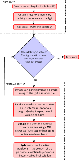
Figure 2: Flow-chart describing the overall structure of AMP. The flow chart assumes that the MINLP is a feasible minimization problem.

AMP consists of two main components. The first component is a presolve (see lines 2 – 5). The presolve component of the algorithm is sub-divided into four parts: (i) computing an initial feasible solution, $\overline{\sigma}$, (line 2), (ii) creating an initial set of partitions, $\bm{\mathcal{I}}$, (iii) sequential OBBT (line 4), and (iv) computing an initial lower bound, $\underline{\sigma}$, using the relaxations detailed in Sec. 2 (line 5).

The second component of AMP is the main loop (lines 6–11) that updates the upper bound, $\overline{\sigma}$, and the lower bound, $\underline{\sigma}$, of $\bm{\mathcal{P}}$, until either of the following conditions are satisfied: the bounds are within $\epsilon$ or the computation time exceeds the limit. At each iteration of the main loop, the partitions are refined and the corresponding piecewise convex relaxation is solved to obtain a lower bound (lines 7 and 8). Similarly the upper bound is obtained using a local solver and updated if it improves the best upper bound computed thus far (lines 9 and 10). In the following sections, we discuss each step of the algorithm in detail.

Algorithm 1 Global optimization using AMP algorithm

1:$\bm{\mathcal{P}}$

2:$\overline{\sigma}\leftarrow$ Solve($\bm{\mathcal{P}}$) $\triangleright$ Compute local optimal solution

3:$\bm{\mathcal{I}}\leftarrow$ InitializePartitions($\bm{\mathcal{P}},\overline{\sigma}$) $\triangleright$ Initialize variable partitions

4:$\bm{x}^{l},\bm{x}^{u}\leftarrow$ TightenBounds($\bm{\mathcal{P}}^{\bm{\mathcal{I}}},\overline{\sigma}$) $\triangleright$ Sequential OBBT

5:$\underline{\sigma}\leftarrow$ Solve($\bm{\mathcal{P}}^{\bm{\mathcal{I}}}$) $\triangleright$ Initial lower bound computation

6:while $\left(\frac{f(\overline{\sigma})-f^{\bm{\mathcal{I}}}(\underline{\sigma})}{f^{\bm{\mathcal{I}}}(\underline{\sigma})}>\epsilon\right)\ \mathrm{and}\ \left(\text{Time}<\text{TimeOut}\right)$ do

7:     $\bm{\mathcal{I}}\leftarrow$ RefinePartitions($\bm{\mathcal{P}}^{\bm{\mathcal{I}}},\underline{\sigma}$) $\triangleright$ Adaptive partition refinement

8:     $\underline{\sigma}\leftarrow$ Solve($\bm{\mathcal{P}}^{\bm{\mathcal{I}}}$) $\triangleright$ Compute new lower bound

9:     $\widehat{\sigma}\leftarrow$ Solve($\bm{\mathcal{P}},\underline{\sigma}$) $\triangleright$ Compute new local optimum

10:     $\overline{\sigma}\leftarrow\arg\min_{\sigma\in\overline{\sigma}\cup\widehat{\sigma}}f(\sigma)$ $\triangleright$ Update upper bound

11:end while

12:$\underline{\sigma},\overline{\sigma}$

3.1 Presolve

The first step of the presolver of AMP is to compute a local optimal solution, $\overline{\sigma}$, to the MINLP (line 2 of Algorithm 1) . This is done using off-the-shelf, open-source solvers that use primal-dual interior point methods in conjunction with a branch-and-bound search tree to handle integer variables. This local solution, $\overline{\sigma}$, is further used to initialize the partitions, $\bm{\mathcal{I}}$ (line 3). When the local solver reports infeasibility, we set the initial value of $f(\overline{\sigma})=\infty$ (line 6) and use the solution obtained by solving the unpartitioned convex relaxation of $\bm{\mathcal{P}}$ to initialize $\bm{\mathcal{I}}$. In the subsequent sections we detail the partition initialization schemes and the sequential OBBT algorithm in lines 3 and 4 of Algorithm 1.

3.1.1 Partition Initialization Scheme and Sequential OBBT

This section details the algorithm used in lines 3 and 4 of AMP’s presolve i.e. InitializePartitions($\bm{\mathcal{P}},\overline{\sigma}$) and TightenBounds($\bm{\mathcal{P}}^{\bm{\mathcal{I}}},\overline{\sigma}$), respectively. The sequential OBBT procedure implemented in these functions is one of the key features of AMP. In many engineering applications there is little or no information about the lower and upper bounds ($\bm{x}^{L},\bm{x}^{U}$) of the decision variables in the problem. Even when known, the gap between the bounds is often large and weaken relaxations. In practice, replacing the original bounds with tighter bounds can (sometimes) dramatically improve the quality of these relaxations. The basic idea of OBBT is the derivation of (new) valid bounds to improve the relaxations. Though, OBBT is a well-known procedure used in global optimization, the key difference is that we apply OBBT sequentially by using mixed-integer models to tighten the bounds.

Algorithm 2 Partition Initialization Scheme

1:function InitializePartitions($\bm{\mathcal{P}},\overline{\sigma}$)

2:     for $i\in 1\ldots n$ do

3:         $\bm{\mathcal{I}}_{i}\leftarrow\{\langle x_{i}^{L},x_{i}^{U}\rangle\}$

4:     end for

5:     if Bound-tightening without partitions then

6:         return $\bm{\mathcal{I}}$

7:     else$\triangleright$ Bound-tightening with partitions

8:         return RefinePartitions($\bm{\mathcal{P}}^{\bm{\mathcal{I}}},\overline{\sigma}$)

9:     end if

10:end function

For the sequential OBBT algorithm we present two procedures. First, OBBT without partitions (BT), which is equivalent to partitioning with a single partition. Second, partition-based OBBT (PBT) which uses the standard partitioning approach described in Section 3.2.1. For simplicity, we drop the term ‘optimization-based (OB)’ in the acronym. The BT uses convex optimization problems to tighten the bounds, while the PBT uses convex MIPs to tighten the bounds. The two procedures differ in the initial set of partitions, $\bm{\mathcal{I}}$, used in the bound-tightening process. Hence, we first present two partition initialization schemes, one for the BT and another for the PBT, respectively. For bound-tightening without partitions, as the name suggests, the partition initialization scheme does not partition the variable domains i.e., $\bm{\mathcal{I}}_{i}\leftarrow\{\langle x_{i}^{L},x_{i}^{U}\rangle\}$ for every $i=1,\dots,n$ (line 6 of Algorithm 2). In the case of PBT, the partition initialization scheme initializes three partitions around the local optimal solution, $\overline{\sigma}$ with a user parameter $\Delta>1$ (line 8 of Algorithm 2 and Section 3.2.1). An illustration of the partitions added to a variable $x\in[x^{L},x^{U}]$, whose value at the local optimal solution is $\overline{\sigma}(x)$, is shown in the Figure 3. If no local solution is obtained in line 2 of Algorithm 1, the solution obtained by solving the unpartitioned convex relaxation of $\bm{\mathcal{P}}$ is used in place of $\overline{\sigma}(x)$.

Figure 3: Partition initialization scheme for PBT.

Once the initial set of partitions is computed, the sequential OBBT procedure iteratively computes new bounds by solving a modified version of $\bm{\mathcal{P}}^{\bm{\mathcal{I}}}$ (Algorithm 3). Each iteration of the sequential OBBT algorithm proceeds as follows: for each continuous variable $x_{i}$ in $\bm{\mathcal{P}}$ appearing in the nonconvex terms, two problems $\bm{\mathcal{P}}^{\bm{\mathcal{I}}}_{l}$ and $\bm{\mathcal{P}}^{\bm{\mathcal{I}}}_{u}$ are solved, where $x_{i}$ is minimized and maximized, respectively, i.e.,

$$\bm{\mathcal{P}}^{\bm{\mathcal{I}}}_{l},\bm{\mathcal{P}}^{\bm{\mathcal{I}}}_{u}:\ \ \ \underset{\bm{x},\bm{y},\widehat{\bm{y}}}{\text{minimize}} \mathbin{\leavevmode\hbox to6.46pt{\vbox to5.98pt{\text{[drawing]}}}}\,x_{i}$$ (8a)

subject to $$f^{\bm{\mathcal{I}}}(\bm{x},\bm{y})\leq f(\overline{\sigma})$$ (8f)

$$\bm{g}^{\bm{\mathcal{I}}}(\bm{x},\bm{y})\leq 0,$$

$$\bm{h}^{\bm{\mathcal{I}}}(\bm{x},\bm{y})=0,$$

$$\bm{x}^{l}_{i}\cdot\widehat{\bm{y}}_{i}\leq x_{i}\leq\bm{x}^{u}_{i}\cdot\widehat{\bm{y}}_{i},\;\;\;\forall\;i=1\ldots n$$

$$\bm{y},\widehat{\bm{y}}\in\{0,1\}$$

where $\mathbin{\leavevmode\hbox to6.46pt{\vbox to5.98pt{\text{[drawing]}}}}\,x_{i}$ in formulation (8) denotes two optimization problems, where $x_{i}$ and $-x_{i}$ are individually minimized (lines 6-7 of Algorithm 3). In both cases, a constraint that bounds the original objective function of $\bm{\mathcal{P}}^{\bm{\mathcal{I}}}$ with a best known feasible solution $\overline{\sigma}$ (equation (8f)) is added when an initial feasible solution is available. Inclusion of this constraint on the objective is referred to as optimality/optimization-based bound-tightening in the literature. The OBBT algorithm stops when cumulative bound improvement between successive iterations, measured in terms of the $\ell^{\infty}$ norm, falls below specified tolerance values (line 3 of Algorithm 3). We note that the sequential OBBT algorithm is naturally parallelizable as all the optimization problems are independently solvable.

Algorithm 3 Sequential bound-tightening of $\bm{x}$

1:function TightenBounds($\bm{\mathcal{P}}^{\bm{\mathcal{I}}},\overline{\sigma}$)

2:     $\widehat{\bm{x}}^{l}=\widehat{\bm{x}}^{u}\leftarrow\bm{0}$

3:     while $||\bm{x}^{l}-\widehat{\bm{x}}^{l}||_{\infty}>\epsilon^{l}$ and $||\bm{\bm{x}}^{u}-\widehat{\bm{x}}^{u}||_{\infty}>\epsilon^{u}$ do

4:         $\widehat{\bm{x}}^{l}\leftarrow\bm{x}^{l},\ \widehat{\bm{x}}^{u}\leftarrow\bm{x}^{u}$

5:         for $i=1,\ldots,n$ do

6:              $\sigma_{i}^{l}\leftarrow$ Solve($\bm{\mathcal{P}}^{\bm{\mathcal{I}}}_{l}$)

7:              $\sigma_{i}^{u}\leftarrow$ Solve($\bm{\mathcal{P}}^{\bm{\mathcal{I}}}_{u}$)

8:              $\bm{x_{i}}^{l}\leftarrow\max(\sigma_{i}^{l}(x_{i}),\bm{x_{i}}^{l})$, $\bm{x_{i}}^{u}\leftarrow\min(\sigma_{i}^{u}(x_{i}),\bm{x_{i}}^{u})$

9:         end for

10:     end while

11:     return $\bm{\bm{x}}^{l},\bm{\bm{x}}^{u}$.

12:end function

Remark 1.

OBBT procedures, usually referred to as domain reduction techniques, are well known in the global optimization literature puranik2017domain ; horst2013handbook . Our algorithm generalizes these techniques by performing optimality-based bound-tightening iteratively based on MIP-formulations (with piecewise convex relaxations) until convergence to a fixed point is achieved.

3.2 Main Algorithm

The main loop of AMP, shown in lines 6 – 11 in Algorithm 1 and main algorithm block of the flow chart in Figure 2, performs three main operations:

1. First, the variable domains are refined adaptively, in a non-uniform manner (line 7 of Algorithm 1).

2. A piecewise convex relaxation is constructed using the partitioned domain, which is solved via outer-approximation to obtain an updated lower bound (line 8 of Algorithm 1)

3. A local solve of the original, MINLP $\bm{\mathcal{P}}$, with the variables bounds restricted to the partitions obtained by the lower bounding solution, is performed to obtain a new local optimal solution. If this solution is better than the current incumbent, then the incumbent is updated (lines 9 and 10 of Algorithm 1).

In the following subsections, we detail each of the three operations involved in the main loop of AMP.

3.2.1 Variable Domain Partitioning

One of the core contributions of the AMP algorithm is the adaptive and non-uniform variable partitioning scheme. This part of the algorithm determines how variables in nonconvex terms of the original MINLP are partitioned. Existing approaches partition each variable domain uniformly into a finite number of partitions and the number of partitions increases with the number of iterations grossmann2013systematic ; bergamini2008improved ; castro2015tightening ; hasan2010piecewise . While this is a straight-forward approach for partitioning the variable domains, it potentially creates huge number of partitions far away from the global optimal value of each variable, i.e., many of the partitions are not useful. Though there have been methods, including sophisticated bound propagation techniques and logarithmic encoding to alleviate this issue, they do not scale to large-scale MINLPs. Instead, our approach successively tightens the relaxations with sparse, non-uniform partitions. This approach focuses partitioning on regions of the variable domain that appear to influence optimality the most. These regions are defined by a solution, $\sigma$, that is typically the lower bound solution at the current iteration.

The adaptive domain partitioning algorithm of AMP refines the variable partitions at a given iteration with a user parameter $\Delta>1$. $\Delta$ is used to control the size and number of the partitions and influences the rate of convergence of the overall algorithm. The algorithm is similar to the algorithm used for initializing the partitions in Section 3.1.1 (see Figure 3). It differs by using the lower bound solution obtained by solving the piecewise relaxations to refine the partition. Again, for the sake of clarity, Figure 4 illustrates the bivariate partition refinement for a bilinear term produced by the adaptive domain partitioning algorithm at successive iterations of the main algorithm. Figure 1(a) geometrically illustrates the tightening of piecewise convex envelopes induced by the adaptive partitioning scheme. The pseudo-code of the domain partitioning algorithm is given in Algorithm 4. The algorithm takes the current variable partitions and a lower bound solution as input and outputs a refined set of partitions for each variable. It first identifies, in line 3 of Algorithm 4, the partition where the lower bound solution is located (active partition) and splits that partition into three new partitions, whose sizes are defined by $\Delta$ and the size of the active partition (lines 7-11 in Algorithm 4).

Exhaustiveness of variable domain partitioning scheme

Exhaustiveness of a partitioning scheme is one of the important requirements for any global optimization algorithm horst2013global . The exhaustiveness of the adaptive domain partitioning scheme is built into AMP through the lines 13 – 14 in Algorithm 4. These conditions ensure that the AMP algorithm does not get stuck at a particular region of the variable. Instead, it guarantees that the largest partition outside the active partition is further refined when the active partition’s width is less than a partition-width tolerance value, $\epsilon^{p}$. Here, the largest inactive partition of a given variable is analogous to the largest unexplored domain for that variable. Thus, the partitioning scheme in the AMP algorithm satisfies the desirable exhaustiveness property.

Algorithm 4 Variable Domain Partitioning

1:function RefinePartitions($\bm{\mathcal{P}}^{\bm{\mathcal{I}}},\sigma$)

2:     for $i\in 1\ldots n$ do

3:         $k\leftarrow\arg\max\sigma(\widehat{y}^{k}_{i})$ $\triangleright$ Identifying the active partition for variable $i$

4:         $\langle l_{i},u_{i}\rangle\leftarrow\bm{\mathcal{I}}_{i}^{k}$

5:         $\xi_{i}\leftarrow\frac{u_{i}-l_{i}}{\Delta}$

6:         if $\xi_{i}>\epsilon^{p}$ then $\triangleright$ Active partition is split into three partitions

7:              $\gamma_{1}\leftarrow\min(l_{i},\max(\sigma(x_{i})-\xi_{i},x_{i}^{L}))$

8:              $\gamma_{2}\leftarrow\max(l_{i},\sigma(x_{i})-\xi_{i})$

9:              $\gamma_{3}\leftarrow\min(u_{i},\sigma(x_{i})+\xi_{i})$

10:              $\gamma_{4}\leftarrow\max(u_{i},\min(\sigma(x_{i})+\xi_{i},x_{i}^{U}))$

11:              $\bm{\mathcal{I}}_{i}\leftarrow(\bm{\mathcal{I}}_{i}\setminus\langle l_{i},u_{i}\rangle)\cup\langle\gamma_{1},\gamma_{2}\rangle\cup\langle\gamma_{2},\gamma_{3}\rangle\cup\langle\gamma_{3},\gamma_{4}\rangle$

12:         else$\triangleright$ Partitioning of largest inactive partition

13:              $\langle l_{i},u_{i}\rangle\leftarrow\arg\max_{\bm{\mathcal{I}}_{i}}u_{i}-l_{i}$

14:              $\bm{\mathcal{I}}_{i}\leftarrow(\bm{\mathcal{I}}_{i}\setminus\langle l_{i},u_{i}\rangle)\cup\langle l_{i},l_{i}+\frac{u_{i}-l_{i}}{2}\rangle\cup\langle l_{i}+\frac{u_{i}-l_{i}}{2},u_{i}\rangle$

15:         end if

16:     end for

17:     return $\bm{\mathcal{I}}$

18:end function

(a) Iteration $k$

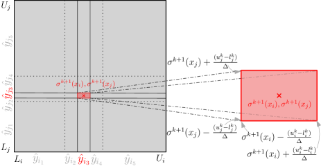
(b) Iteration $k+1$

Figure 4: Adaptive partitioning strategy for a bilinear function $x_{i}x_{j}$ as described in Algorithm 4. Red and gray colored boxes represent active and inactive partitions, respectively. $k$ and $k+1$ refer to successive solutions used to partition the active partition.

3.2.2 Computing Lower and Upper Bounds

Once the variable partitions are refined, the main loop of the AMP algorithm constructs and solves a piecewise convex relaxation, $\bm{\mathcal{P}}^{\bm{\mathcal{I}}}$ (line 8 of Algorithm 1). Each $\bm{\mathcal{P}}^{\bm{\mathcal{I}}}$ is a convex MIP where all the constraints are either linear or second-order cones (SOCs). Theoretically, $\bm{\mathcal{P}}^{\bm{\mathcal{I}}}$ can be solved by off-the-shelf mixed-integer, conic solvers. However, initial computational experiments suggested that several moderately sized problems with SOC constraints were difficult to solve, even with state-of-the-art solvers. It was the case that either the solver convergence was very slow or the solve terminated with a numerical error. To circumvent this issue and solve these convex MIPs in a computationally efficient manner, the SOC constraints in the convex MIP were outer-approximated via first-order approximations, using the lazy-callback feature in the MIP solvers.

To obtain a new local optimal solution in the main loop of AMP (line 9 of Algorithm 1), the feasible solution is obtained by solving the NLP, $\bm{\mathcal{P}}^{u}$, shown in Eq. (9). $\bm{\mathcal{P}}^{u}$ is constructed at each iteration of the main loop using the original MINLP, $\bm{\mathcal{P}}$, and the lower bound solution computed at that iteration, $\underline{\sigma}$.

$$\bm{\mathcal{P}}^{u}:\ \ \ \underset{\bm{x},\bm{y}}{\text{minimize}} f(\bm{x},\bm{y})$$ (9a)

subject to $$\bm{g}(\bm{x},\bm{y})\leq 0,$$ (9e)

$$\bm{h}(\bm{x},\bm{y})=0,$$

$$\bm{x}^{l}_{i}\cdot\underline{\sigma}(\widehat{\bm{y}}_{i})\leq{x}_{i}\leq\bm{x}^{u}_{i}\cdot\underline{\sigma}(\widehat{\bm{y}}_{i}),\;\;\;\forall\;i=1\ldots n$$

$$\bm{y}=\underline{\sigma}(\bm{y})$$

where constraint (9e) forces the variable assignments into the partition defined by the current lower bound. Constraint (9e) fixes all the original binary variables to the lower bound solution. $\bm{\mathcal{P}}^{u}$ is then solved to local optimality using a local solver. The motivation for this approach is based on empirical observations that the relaxed solution is often very near to the global optimum solution and that the NLP is solved fast once all binary variables are fixed to constant values. $\bm{\mathcal{P}}^{u}$ is essentially a projection of the relaxed solution (lower bound solution, $\underline{\sigma}$) back onto a near point in the feasible region of $\bm{\mathcal{P}}$; this approach is often used for recovering feasible solutions bergamini2008improved . In the forthcoming Lemma 2, we claim that the value of the objective function of the piecewise convex relaxation at each iteration monotonically increases to the global optimum solution with successive partition refinements.

Lemma 2.

Let $\underline{\sigma}^{\bm{\mathcal{I}}}$ denote the optimal solution to the formulation $\bm{\mathcal{P}}^{\bm{\mathcal{I}}}$ and let $\sigma^{*}$ denote the global optimal solution to $\bm{\mathcal{P}}$. Then, $f^{\bm{\mathcal{I}}}(\underline{\sigma}^{\bm{\mathcal{I}}})$ monotonically increases to $f(\sigma^{*})$ as $|\bm{\mathcal{I}}_{i}|\rightarrow\infty$ for every $i=1,\dots,n$.

Proof.

Without loss of generality, we assume $\bm{\mathcal{P}}$ is feasible and restrict our discussion to bilinear terms. Let $x_{i}x_{j}$ be a bilinear term. Given a finite set of partitions, that is, $1\leqslant|\bm{\mathcal{I}}_{i}|,|\bm{\mathcal{I}}_{j}|<\infty$, there always exists a partition in $\bm{\mathcal{I}}_{i}$ and $\bm{\mathcal{I}}_{j}$ that is active in the solution to $\bm{\mathcal{P}}^{\bm{\mathcal{I}}}$. Let the active partitions have lengths $\epsilon^{l}_{i}+\epsilon^{u}_{i}$ and $\epsilon^{l}_{j}+\epsilon^{u}_{j}$, respectively. Given the exhaustiveness property of the adaptive partitioning scheme discussed in section 3.2.1, assume the active partition contains the global optimum solution $\sigma^{*}({\bf x}^{*},{\bf y}^{*})$. Then, we have

$$x^{*}_{i}-\epsilon^{l}_{i}\leqslant x_{i}\leqslant x^{*}_{i}+\epsilon^{u}_{i},\quad x^{*}_{j}-\epsilon^{l}_{j}\leqslant x_{j}\leqslant x^{*}_{j}+\epsilon^{u}_{j}.$$

For these active partitions, the McCormick constraints in (4a) and (4c) linearize $x_{i}x_{j}$ as follows:

$$\widehat{x_{ij}} \geqslant(x^{*}_{i}-\epsilon^{l}_{i})x_{j}+(x^{*}_{j}-\epsilon^{l}_{j})x_{i}-(x^{*}_{i}-\epsilon^{l}_{i})(x^{*}_{j}-\epsilon^{l}_{j})$$ (10)

$$=(x_{i}^{*}x_{j}+x_{j}^{*}x_{i}-x_{i}^{*}x_{j}^{*})+\underbrace{\epsilon^{l}_{i}(x_{j}^{*}-x_{j})+\epsilon^{l}_{j}(x_{i}^{*}-x_{i})-\epsilon^{l}_{i}\epsilon^{l}_{j}}_{\mathcal{E}(\epsilon_{i}^{l},\epsilon_{j}^{l})}$$

and

$$\widehat{x_{ij}} \leqslant(x^{*}_{i}-\epsilon^{l}_{i})x_{j}+(x^{*}_{j}+\epsilon^{u}_{j})x_{i}-(x^{*}_{i}-\epsilon^{l}_{i})(x^{*}_{j}+\epsilon^{u}_{j})$$ (11)

$$=(x_{i}^{*}x_{j}+x_{j}^{*}x_{i}-x_{i}^{*}x_{j}^{*})+\underbrace{\epsilon^{l}_{i}(x_{j}^{*}-x_{j})+\epsilon^{u}_{j}(x_{i}-x_{i}^{*})+\epsilon^{l}_{i}\epsilon^{u}_{j}}_{\mathcal{E}(\epsilon_{i}^{l},\epsilon_{j}^{u})}$$

where, $\mathcal{E}(\epsilon_{i}^{l},\epsilon_{j}^{l})<0$ and $\mathcal{E}(\epsilon_{i}^{l},\epsilon_{j}^{u})>0$ are the error terms of the under- and over-estimator, respectively. It is trivial to observe that the error terms themselves constitute the McCormick envelopes of $(x_{i}^{*}-x_{i})(x_{j}^{*}-x_{j})$ if one were to linearize this product. Further, observing that the error terms, as described above, are parametrized by the size of the active partition containing the global optimum point, given by $\epsilon_{i}^{l}+\epsilon_{i}^{u}$ and $\epsilon_{j}^{l}+\epsilon_{j}^{u}$, for variables $x_{i}$ and $x_{j}$, respectively, we now derive the analytic forms of these terms as a function of the total number of partitions for the adaptive partitioning case.

Line 7 in Algorithm 1 ensures that the partitions created during the $(k+1)^{th}$ iteration of the main loop for either of the variables, $x_{i}$ or $x_{j}$, is a subset of the partitions created for the corresponding variables in the $k^{th}$ iteration. Also, for a $k^{th}$ iteration of an adaptive refinement step for variables $x_{i}$ and $x_{j}$, we assume that at most $3+2(k-1)$ partitions exist within the given variable bounds ($L_{i},U_{i}$) and ($L_{j},U_{j}$), respectively. Thus, the length of the above mentioned active partition which contains the global solution is given by

$$\epsilon_{i}^{l}+\epsilon_{i}^{u}=\frac{U_{i}-L_{i}}{\Delta^{\frac{|\bm{\mathcal{I}}_{i}|-1}{2}}},\quad\epsilon_{j}^{l}+\epsilon_{j}^{u}=\frac{U_{j}-L_{j}}{\Delta^{\frac{|\bm{\mathcal{I}}_{j}|-1}{2}}}.$$

Clearly as $|\bm{\mathcal{I}}_{i}|$ and $|\bm{\mathcal{I}}_{j}|$ approach $\infty$, the error terms of the McCormick envelopes, $\mathcal{E}(\epsilon_{i}^{l},\epsilon_{j}^{l})$ and $\mathcal{E}(\epsilon_{i}^{l},\epsilon_{j}^{u})$, approach zero, and thus enforcing $x_{i}=x_{i}^{*}$, $x_{j}=x_{j}^{*}$ and $\widehat{x_{ij}}=x_{i}^{*}x_{j}^{*}$. Therefore, as $|\bm{\mathcal{I}}_{i}|$ approaches $\infty$ for every variable $i$ that is partitioned, $f^{\bm{\mathcal{I}}}(\underline{\sigma}^{\bm{\mathcal{I}}})$ approaches the global optimal solution $f(\sigma^{*})$.

Also observe that since $\mathfrak{F}(\bm{\mathcal{P}}^{\bm{\mathcal{I}}})\subset\mathfrak{F}(\bm{\mathcal{P}})$ for any finite $\bm{\mathcal{I}}$, $f^{\bm{\mathcal{I}}}(\underline{\sigma}^{\bm{\mathcal{I}}})\leqslant f(\sigma^{*})$. Here, $\mathfrak{F}(\cdot)$ denotes the feasible space of the formulation of “$\cdot$”. Furthermore, the partition set in iteration $k$ is a proper subset of the previous iteration’s partitions. This proves the monotonicity of the sequence of values $f^{\bm{\mathcal{I}}}(\underline{\sigma}^{\bm{\mathcal{I}}})$ with increasing iterations of the main loop of AMP. ∎

4 Computational results

In the remainder of this paper, we refer to AMP as Algorithm 1 without the implementation of line 3, i.e., without any form of sequential OBBT. BT-AMP and PBT-AMP refer to Algorithm 1 implemented with bound-tightening without and with partitions added, respectively. The performance of these algorithms is evaluated on a set of standard benchmarks from the literature with mutlilinear terms. These problems include a small NLP that is used to highlight the differences between the sparse, adaptive approaches and uniform partitioning approaches. The details and sources for each problem instance are shown later in this section in Table 7. In this table, we also mention the continuous variables in mutlilinear terms chosen for partitioning. Ipopt 3.12.8 and Bonmin 1.8.2 are used as local NLP and MINLP solvers for the feasible solution computation in AMP, respectively. MILPs and MIQCQCPs are solved using CPLEX 12.7 (cpx) and/or Gurobi 7.0.2 (grb) with default options and presolver switched on. The outer-approximation algorithm was implemented using the lazy callback feature of CPLEX and Gurobi. Given that the bound-tightening procedure consists of independently solvable problems, 10 parallel threads were used during bound-tightening. In the Appendix we provide a detailed sensitivity analysis of the parameters of AMP.

Every bound-tightening (BT and PBT) problem was solved to optimality (except meyer15). For meyer15, 0.1% optimality gap was used as a termination criteria because it is a large-scale MINLP.The value of $\epsilon$ and the “TimeOut” parameter in Algorithm 1 were set to $0.0001$ and $3600$ seconds, respectively. However, for BT and PBT, we did not impose any time limit. Thus, for a fair comparison, we set the time limit for the global solver to be the sum of bound tightening time and 3600 seconds (denoted by $T^{+}$ in the tables). In the results, “TO” indicates that the AMP solve timed-out. All results are benchmarked with BARON 17.1, a state-of-the-art global optimization solver sahinidis1996baron ; tawarmalani2005polyhedral . CPLEX 12.7 and Ipopt 3.12.8 are used as the underlying MILP and non-convex local solvers for BARON. JuMP, an algebraic modeling language in Julia dunning2017jump , was used for implementing all the algorithms and invoking the optimization solvers. All the computational experiments were performed using the high-performance computing resources at the Los Alamos National Laboratory with Intel CPU E5-2660-v3, Haswell micro-architecture, 20 cores (2 threads per core) and 125GB of memory.

4.1 Performance on a Small-scale NLP

$$\mathit{NLP1:} \underset{x_{1},\ldots,x_{8}}{\text{minimize}} x_{1}+x_{2}+x_{3}$$

subject to $$0.0025(x_{4}+x_{6})-1\leq 0,$$

$$0.0025(-x_{4}+x_{5}+x_{7})-1\leq 0,$$

$$0.01(-x_{5}+x_{8})-1\leq 0,$$

$$100x_{1}-x_{1}x_{6}+833.33252x_{4}-83333.333\leq 0,$$

$$x_{2}x_{4}-x_{2}x_{7}-1250x_{4}+1250x_{5}\leq 0,$$

$$x_{3}x_{5}-x_{3}x_{8}-2500x_{5}+1250000\leq 0,$$

$$100\leq x_{1}\leq 10000,$$

$$1000\leq x_{2},x_{3}\leq 10000,$$

$$10\leq x_{4},x_{5},x_{6},x_{7},x_{8}\leq 1000$$

In this section, we perform a detailed study of AMP with and without OBBT on NLP1, a small-scale, continuous nonlinear program adapted from Problem 106 in hock1980test . This small problem helps illustrate many of the salient features of AMP. NLP1 has gained considerable interest from the global optimization literature due its large variable bounds and weak McCormick relaxations. Since this is a challenging problem for uniform, piecewise McCormick relaxations, this problem has been studied in detail in castro2015tightening ; castro2015normalized ; teles2013univariate . The value of the global optimum for NLP1 is 7049.2479 and the solution is $x^{*}_{i},\ i=1,\ldots,8=[579.307,1359.97,5109.97,182.018,295.601,217.982,286.417,395.601]$.

4.1.1 AMP versus Uniform Partitioning on NLP1

Figure 5 compares AMP (without BT/PBT) with a uniform partitioning strategy that is often used in state-of-the-art solvers to obtain global solutions. For a fair comparison, we used the same number of partitions for both methods at every iteration. From Figure 5(a), it is evident that AMP exhibits larger optimality gaps in the first few iterations (134%, 44%, 20%, vs. 97%, 44%, 16%, etc.). However, the convergence rate to global optimum is much faster with AMP (within 190.9 seconds). This behaviour is primarily attributed to the adaptive addition of partitions around the best-known local solution (also global in this case) instead of spreading them uniformly.

(a) Optimality gap

(b) Cumulative time

Figure 5: Performance of AMP ($\Delta=4$) and uniform partitioning on NLP1. Note that the y-axis is on log scale.

4.1.2 Performance of AMP on NLP1

Figure 6 shows the active partitions chosen by every iteration of AMP for $\Delta=4$. This figure illustrates the active partitions at each iteration of the main loop of AMP and the convergence of each variable partition to its corresponding global optimal value. One of the primary motivations of the adaptive partitioning strategy comes from the observation that every new partition added adaptively refines the regions (hopefully) closer to the global optimum values. In Figure 6(a), this behaviour is clearly evident on all the variables except $x_{3}$. Although the initial active partition on $x_{3}$ did not contain the global optimum, AMP converged to the global optimum value. The convergence time of AMP to the global optimum using Gurobi was 190.9 seconds. The total number of binary partitioning variables is 152 (19 per continuous variable).

(a) Variables $x_{1},x_{3}$

(b) Variables $x_{2},x_{4}$

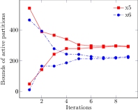
(c) Variables $x_{5},x_{6}$

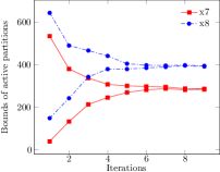
(d) Variables $x_{7},x_{8}$

Figure 6: Upper and lower bounds of active partitions chosen by AMP algorithm (without OBBT) for the variables $x_{i},i=1,\ldots,8$ of NLP1.

4.1.3 Benefits of MIP-based OBBT on NLP1

(a) Tightened bounds after each iteration

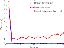
(b) Time per iteration

Figure 7: Performance of sequential BT and sequential PBT techniques on NLP1.

Table 1: Contracted bounds after applying sequential bound tightening to nlp1.

	Original bounds		PBT bounds		#BVars added
Variable	$L$	$U$	$l$	$u$	BT, AMP	PBT, AMP
					($\Delta=4$)	($\Delta=4$)
$x_{1}$	100	10000	573.1	585.1	0, 14	3, 3
$x_{2}$	1000	10000	1351.2	1368.5	0, 14	3, 3
$x_{3}$	1000	10000	5102.1	5117.5	0, 15	3, 3
$x_{4}$	10	1000	181.5	182.5	0, 15	3, 3
$x_{5}$	10	1000	295.3	296.0	0, 15	3, 3
$x_{6}$	10	1000	217.5	218.5	0, 15	3, 3
$x_{7}$	10	1000	286.0	286.9	0, 15	3, 3
$x_{8}$	10	1000	395.3	396.0	0, 15	3, 3
Total					118	48

Figure 7 and Table 1 show the effectiveness of sequential BT and sequential PBT techniques on NLP1. As expected, in Figure 7(a), the disjunctive polyhedral representation of the relaxed regions in PBT (around the initial local solution) drastically reduce the global bounds on the variables (to almost zero gaps). Figure 7(b) shows that PBT, even when solving a MILP in every iteration, does not incur too much computational overhead on a small-scale problem like NLP1.

A qualitative description of the improved performance is presented in Table 1. The column titled “#BVars added” shows the total number of partitions that were added for each variable for BT-AMP and PBT-AMP. While BT adds no partitions and AMP adds a total of 118 partitions, PBT adds a total of 24 partitions in addition to 24 more partitions during AMP. As is seen in the results in the “PBT bounds” column, the bounds of the variables are tightened to near global optimum values and AMP needs very few additional partitions to prove global optimality within 40 seconds. In contrast, AMP adds a lot more partitions as the bounds of the variables after BT are not tight enough. Overall, for NLP1, it is noteworthy that PBT-AMP outperforms most of the state-of-the-art piecewise relaxation methods developed in the literature.

4.2 Performance of AMP on Large-scale MINLPs

Table 2: Summary of the performance of AMP without OBBT on all instances. Here, we compare the run times of BARON, AMP with $\Delta=8$ (cpx), AMP with the best $\Delta$ (cpx) and AMP with the best $\Delta$ (grb). Values under “Gap” and “$T$” are in % and seconds, respectively. “Inf” implies that the solver failed to provide a bound within the prescribed time limit. For each instance, the bold face font represents best run time or the best optimality gap (if the solve times out)

	COUENNE		BARON		AMP-cpx		AMP-cpx			AMP-grb
					$\Delta=8$		$\Delta^{*}$			$\Delta^{*}$
Instances	Gap	$T$	Gap	$T$	Gap	$T$	$\Delta$	Gap	$T$	$\Delta$	Gap	$T$
p1	GOpt	0.01	GOpt	0.02	GOpt	0.26	32	GOpt	0.19	32	GOpt	0.06
p2	GOpt	0.01	GOpt	0.01	GOpt	0.05	16	GOpt	0.03	32	GOpt	0.10
fuel	Inf	N/A	GOpt	0.03	GOpt	0.07	4	GOpt	0.03	4	GOpt	0.05
ex1223a	GOpt	0.01	GOpt	0.02	GOpt	0.01	32	GOpt	0.01	16	GOpt	0.02
ex1264	GOpt	2.04	GOpt	1.44	GOpt	1.42	16	GOpt	0.90	8	GOpt	0.79
ex1265	GOpt	5.22	GOpt	13.30	GOpt	0.94	16	GOpt	0.17	8	GOpt	0.28
ex1266	GOpt	5.37	GOpt	10.81	GOpt	0.27	32	GOpt	0.14	32	GOpt	0.16
eniplac	GOpt	128.82	GOpt	207.37	GOpt	1.17	32	GOpt	0.68	32	GOpt	0.75
util	GOpt	14.56	GOpt	0.10	GOpt	1.21	16	GOpt	0.54	16	GOpt	0.55
meanvarx	GOpt	1.06	GOpt	0.05	GOpt	290.61	16	GOpt	95.51	16	GOpt	70.09
blend029	GOpt	35.18	GOpt	2.46	GOpt	1.74	32	GOpt	0.74	32	GOpt	1.00
blend531	3.06	TO	GOpt	111.79	GOpt	185.33	8	GOpt	185.33	16	GOpt	49.76
blend146	4.19	TO	2.20	TO	2.01	TO	8	2.01	TO	8	1.60	TO
blend718	156.45	TO	175.10	TO	GOpt	379.58	8	GOpt	379.58	8	GOpt	581.68
blend480	102.41	TO	GOpt	326.95	0.32	TO	32	0.04	TO	16	0.02	TO
blend721	0.60	TO	GOpt	548.90	GOpt	504.74	32	GOpt	256.77	16	GOpt	176.11
blend852	1.74	TO	0.08	TO	GOpt	750.88	4	GOpt	169.24	16	GOpt	322.80
wtsM2_05	GOpt	3426.28	GOpt	153.30	20.08	TO	8	20.08	TO	32	GOpt	386.95
wtsM2_06	31.95	TO	GOpt	228.18	8.76	TO	4	GOpt	2395.71	32	GOpt	972.20
wtsM2_07	GOpt	68.37	GOpt	759.96	0.10	TO	8	0.10	TO	16	0.54	TO
wtsM2_08	39.43	TO	388.62	TO	9.82	TO	4	5.45	TO	4	7.92	TO
wtsM2_09	60.37	TO	Inf	TO	68.58	TO	10	36.47	TO	4	7.47	TO
wtsM2_10	0.64	TO	76.48	TO	35.88	TO	32	24.95	TO	16	0.10	TO
wtsM2_11	64.71	TO	107.56	TO	7.88	TO	16	3.50	TO	4	6.10	TO
wtsM2_12	68.56	TO	85.35	TO	8.07	TO	4	7.46	TO	32	4.00	TO
wtsM2_13	47.74	TO	54.04	TO	10.06	TO	4	4.24	TO	8	5.72	TO
wtsM2_14	47.15	TO	46.24	TO	9.02	TO	32	6.34	TO	16	1.43	TO
wtsM2_15	61.32	TO	Inf	TO	86.64	TO	4	8.81	TO	8	0.22	TO
wtsM2_16	26.72	TO	47.77	TO	34.46	TO	8	34.46	TO	32	5.25	TO
lee1	GOpt	46.97	GOpt	145.55	GOpt	13.01	8	GOpt	13.01	8	GOpt	13.61
lee2	GOpt	60.43	GOpt	590.08	0.58	TO	16	0.47	TO	16	0.08	TO
meyer4	Inf	N/A	80.40	TO	GOpt	18.85	4	GOpt	12.50	8	GOpt	5.68
meyer10	80.88	TO	239.70	TO	GOpt	TO	4	GOpt	452.53	8	GOpt	133.47
meyer15	Inf	N/A	2850.30	TO	0.59	TO	16	0.31	TO	4	0.10	TO

In this section we assess the empirical value of adaptive partitioning by presenting results without OBBT. In Table 2, AMP (without OBBT) with CPLEX or Gurobi is compared with BARON. Columns two and three show the run times of Couenne and BARON, respectively, based on the 3600 second time limit. Column four shows the performance of AMP for $\Delta=8$. Though $\Delta=8$ is not the ideal setting for every instance, it is analogous to running BARON/Couenne with default parameters. Under the default AMP settings, AMP is faster than BARON and Couenne (with default settings) at finding the best lower bound in 23 out of 34 instances. These results of AMP are the most fair to compare with untuned BARON and Couenne

In column five (tuned $\Delta$ and CPLEX), the run times of AMP are much faster than BARON and Couenne in 24 out of 34 instances. Column six (tuned $\Delta$ and Gurobi) again indicates that the right choice of $\Delta$ speeds up the convergence of AMP drastically. More interestingly, on 21 out of 34 instances, the run times of AMP using Gurobi are substantially better than the run times using CPLEX (column 5).

Table 2 is summarized with a cumulative distribution plot in Figure 8. Clearly, Figure 8(a) indicates that AMP is better able to find solutions within a 0.4% optimality gap (even without tuning). Figure 8(b) provides evidence of the overall strength of AMP. Even when AMP is not the fastest approach, its run times are very similar to BARON. Overall, the performance of AMP is clearly better using Gurobi as the underlying MILP/MIQCQP solver. We did not perform comparative studies of BARON with Gurobi because it cannot currently integrate with Gurobi.

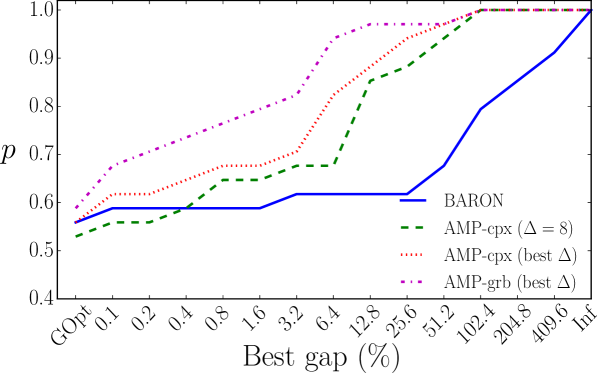
(a) Comparison of best gap

(b) Comparison of best run times

Figure 8: Performance profiles of AMP (without OBBT) and BARON. In (a), the x axis plots the optimality gap of the algorithms and the y axis plots fraction of instances. Plot (a) tracks the number of instances where an algorithm is able achieve the specified optimality gap. In (b), the x axis denotes the run time ratio of an algorithm with the best run time of any algorithm. The y axis denotes the fraction of instances. Plot (b) tracks the number of times an algorithm’s run time is within a specified factor of the best run time of any algorithm. In both figures, higher is better. Overall, AMP performs better than BARON on a $p$ proportion of instances for most gaps and all run times.

4.3 Performance of AMP with OBBT

We next discuss the performance of AMP when OBBT is added.

4.3.1 Default Parameters of $\Delta$

We first consider AMP with OBBT when AMP uses the default parameter of $\Delta=8$. Table 3, compares AMP with BARON. Column two shows the run times of BARON based on a prescribed time limit. For comparison purposes with AMP, the time limit of BARON is calculated as the sum of 3600 seconds and the maximum of the run time of BT and PBT. For the purposes of this study, we did not specify a time limit on BT and PBT, though this could be added.

Column three shows the performance of BT-AMP when $\Delta=8$. While a constant $\Delta$ is not the ideal parameter for every instance, BT-AMP with CPLEX is still faster than BARON on 21 out of 32 instances. Similarly, BT-AMP with Gurobi is faster in 25 out of 32 instances. Once again, AMP with Gurobi has significant computational advantages over CPLEX. Instances blend480, blend721, blend852, and meyer10 demonstrated an order of magnitude improvement. Column four of Table 3 shows the results of PBT-AMP when $\Delta=10$. Though PBT solves a more complicated, discrete optimization problem at every step of bound-tightening, surprisingly, the total time spent in bound-tightening was typically significantly smaller. This is seen in all instances prefixed with “ex”, the util instance, the eniplac instance, the meanvarx instance and a few blend instances. In general, using partition-based OBBT yields significant improvements in the overall run times and optimality gaps of AMP.

The bound-tightening procedure also compares favorably with BARON. For example, consider problem blend852. Though BARON implements a sophisticated bound-tightening approach that is based on primal and dual formulations, BARON times out with a 0.08% gap. In contrast, BT-AMP with Gurobi converges to the global optimum in 434.7 seconds and PBT-AMP converges to the global optimum in 78.1 seconds (an order-of-magnitude improvement). Similar behaviour is observed on the remaining blend, wts and meyer instances. Overall, AMP with Gurobi outperforms BARON on 24 out of 32 instances when a default choice of $\Delta$ is used.

Table 3 is summarized with a cumulative distribution plot in Figure 9. Clearly, Figure 9(a) indicates that BT-AMP and PBT-AMP with Gurobi performs better than BARON even without tuning $\Delta$. In 9(a), AMP has a better profile when the optimality gap is $>0.4\%$. In Figure 9(a), the performance improvement starts at $0.2\%$. However, there is an increase in run times due to bound-tightening (Figure 9(b)), that allows to AMP to achieve this improvement.

Remark 2.

meyer15, a generalized pooling problem-based instance, is classified as a large-scale MINLP and is very hard for global optimization. The current best known gap for this instance is 0.1% misener2011apogee ; bussieck2003minlplib . PBT-AMP with Gurobi has closed this problem by proving the global optimum for the first time (943734.0215–Table 3).

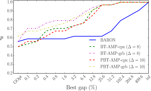
(a) Comparison of best gap

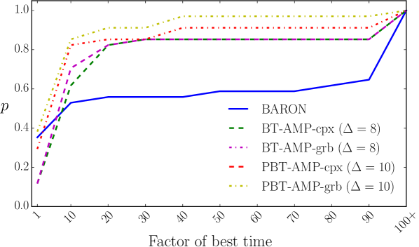
(b) Comparison of best run times

Figure 9: Performance profiles of AMP (with OBBT) and BARON. In (a), the x axis plots the optimality gap of the algorithms and the y axis plots fraction of instances. Plot (a) tracks the number of instances where an algorithm is able achieve the specified optimality gap. In (b), the x axis denotes the run time ratio of an algorithm with the best run time of any algorithm. The y axis denotes the fraction of instances. Plot (b) tracks the number of times an algorithm’s run time is within a specified factor of the best run time of any algorithm. In both figures, higher is better. Overall, AMP performs better than BARON on $p$ proportion of instances within a factor of the best gap and with the best run times.

Table 3: Performance summary of AMP with OBBT on all instances. Here, we compare the run times of BARON, BT-AMP with $\Delta=8$ and PBT-AMP with $\Delta=10$. CPLEX and Gurobi are the underlying solvers for AMP. Values under “Gap” and “$T,T^{+}$” are in % and seconds, respectively.“Inf” implies that the solver failed to provide a bound within the prescribed time limit.

	BARON		BT	AMP-cpx		AMP-grb		PBT	AMP-cpx		AMP-grb
Instances	Gap	$T$	$T^{+}$	Gap	$T$	Gap	$T$	$T^{+}$	Gap	$T$	Gap	$T$
fuel	GOpt	0.03	0.01	GOpt	0.03	GOpt	0.03	0.01	GOpt	0.04	GOpt	0.03
ex1223a	GOpt	0.02	19.71	GOpt	0.01	GOpt	0.01	0.30	GOpt	0.01	GOpt	0.02
ex1264	GOpt	1.44	12.47	GOpt	1.77	GOpt	1.32	0.72	GOpt	1.48	GOpt	1.24
ex1265	GOpt	13.3	6.02	GOpt	0.25	GOpt	0.88	1.02	GOpt	0.26	GOpt	0.74
ex1266	GOpt	10.81	13.75	GOpt	0.12	GOpt	0.06	1.30	GOpt	0.04	GOpt	0.06
eniplac	GOpt	207.37	16.04	GOpt	1.13	GOpt	1.36	3.34	GOpt	1.17	GOpt	1.59
util	GOpt	0.10	9.92	GOpt	0.17	GOpt	0.19	0.61	GOpt	0.14	GOpt	0.16
meanvarx	GOpt	0.05	20.69	GOpt	95.23	GOpt	59.33	3.53	GOpt	13.62	GOpt	13.31
blend029	GOpt	2.46	15.05	GOpt	1.04	GOpt	1.56	0.80	GOpt	0.88	GOpt	0.95
blend531	GOpt	111.79	44.67	GOpt	38.60	GOpt	22.56	477.94	GOpt	39.89	GOpt	20.12
blend146	2.20	TO	30.95	24.92	TO	0.10	TO	26.66	24.98	TO	23.69	TO
blend718	175.10	TO	28.76	GOpt	1332.66	GOpt	1335.93	20.8	14.65	TO	GOpt	868.14
blend480	GOpt	326.95	137.62	0.21	TO	GOpt	108.93	1699.18	8.78	TO	GOpt	2466.17
blend721	GOpt	548.9	29.44	GOpt	646.92	GOpt	181.88	23.92	GOpt	93.28	GOpt	112.91
blend852	0.08	TO	41.73	GOpt	749.03	GOpt	392.99	29.40	GOpt	217.62	GOpt	48.79
wtsM2_05	GOpt	153.30	14.82	0.24	TO	0.02	TO	0.34	0.22	TO	GOpt	2875.17
wtsM2_06	GOpt	228.18	15.52	0.01	TO	0.01	TO	0.33	0.02	TO	GOpt	1957.59
wtsM2_07	GOpt	759.96	16.15	0.26	TO	0.30	TO	0.22	0.04	TO	1.59	TO
wtsM2_08	388.62	TO	21.54	14.37	TO	14.72	TO	0.90	20.08	TO	19.94	TO
wtsM2_09	Inf	TO	42.28	61.99	TO	64.53	TO	13.96	56.72	TO	55.85	TO
wtsM2_10	76.48	TO	15.73	0.10	TO	0.07	TO	0.32	0.22	TO	0.22	TO
wtsM2_11	107.56	TO	22.64	9.76	TO	3.74	TO	1.09	13.81	TO	9.18	TO
wtsM2_12	85.35	TO	39.10	11.90	TO	11.92	TO	3.44	6.03	TO	11.02	TO
wtsM2_13	54.04	TO	111.39	2.01	TO	3.95	TO	17.00	2.17	TO	2.10	TO
wtsM2_14	46.24	TO	19.09	6.64	TO	4.71	TO	1.10	1.93	TO	1.93	TO
wtsM2_15	Inf	TO	14.93	0.29	TO	0.50	TO	0.34	0.51	TO	0.48	TO
wtsM2_16	47.77	TO	22.54	8.76	TO	6.91	TO	1.18	9.40	TO	5.11	TO
lee1	GOpt	145.55	13.28	GOpt	12.50	GOpt	13.55	0.22	10.00	TO	0.01	TO
lee2	GOpt	590.08	14.92	0.58	TO	0.37	TO	5.35	0.43	TO	0.07	TO
meyer4	80.40	TO	15.78	GOpt	4.22	GOpt	4.47	238.47	GOpt	14.76	GOpt	13.68
meyer10	239.70	TO	44.68	9.74	TO	GOpt	2925.36	63.79	GOpt	TO	GOpt	1189.71
meyer15	2556.37	TO	3877.09	3.44	TO	0.08	TO	17868.96	GOpt	TO	GOpt	TO

4.3.2 Tuned $\Delta$ Parameter

In Table 4, we show the results of AMP (with OBBT) when $\Delta$ is tuned for each problem instance and these results are compared with BARON. For the purposes of this article, $\Delta$ is tuned by running AMP with $\Delta=\{4,8,10,16,32\}$ on each instance. We then choose the value of $\Delta$ that provides the best lower bound (global optimal in many cases) in the minimum amount of computation time. This tuned value of $\Delta$ is denoted by $\Delta^{*}$ in Table 4. Developing adaptive and automatic tuning heuristic-algorithms for computing the value of $\Delta$ remains an open question and is a subject of future work. As the performance of AMP is consistently the strongest with Gurobi, we present those results. Overall, this table shows the best results for AMP. Column two of this table shows the run times of BARON. Similar to table 3, the time limit for BARON is the sum of 3600 seconds and the maximum of the run times of the BT and PBT algorithms (no time limit on BT and PBT). Column three tabulates the performance of BT-AMP with Gurobi by choosing the best $\Delta$ parameter for each instance. Overall, BT-AMP and PBT-AMP performed better than BARON on 26 out of 32 instances. As discussed in detail in section 4.3.1, similar observations about the performance of our algorithms also hold for this table. Again, the performance of PBT, despite the use of discrete optimization, indicates that PBT is the strongest bound-tightening procedure. On the large MINLP instance meyer15, PBT has large computational overhead, but this overhead pays off when AMP converges to the global optimum in 538.56 seconds. As noted in the earlier remark, this was an open instance prior to this work.

Table 3 is summarized with the cumulative distribution plot shown in Figure 10. Figure 10(a) indicates that AMP, BT-AMP and PBT-AMP with Gurobi are better than BARON in finding the best lower bounds. Though the proportion of instances for which global optima are attained is not significantly different than BARON, the proportion of instances for which better lower bounds are found using AMP-based algorithms is larger. Also, the advantages of BT and PBT-based bound-tightening in AMP is evident from the fact that the proportion of instances that find global optimum is higher. As expected, Figure 10(b) suggests that AMP with Gurobi is overall faster than BARON on the easiest instances, but on harder instances this speed is tempered by a degradation in solution quality.

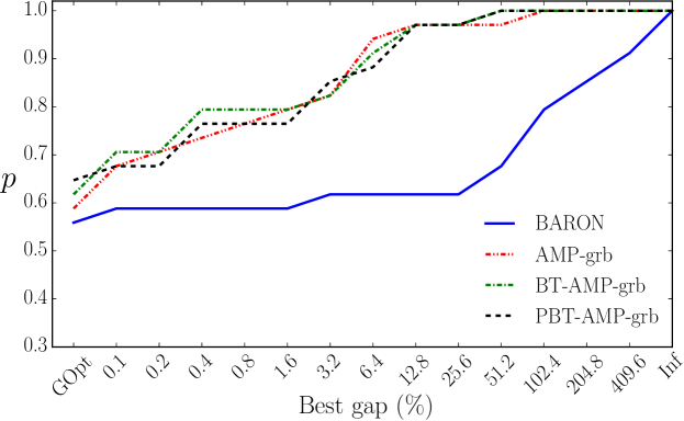
(a) Comparison on Best Gap %

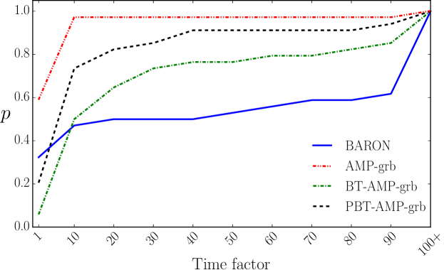
(b) Comparison on Best CPU Times

Figure 10: Performance profiles of AMP (with OBBT and tuned $\Delta$) and BARON. In (a), the x axis plots the optimality gap of the algorithms and the y axis plots fraction of instances. Plot (a) tracks the number of instances where an algorithm is able achieve the specified optimality gap. In (b), the x axis denotes the run time ratio of an algorithm with the best run time of any algorithm. The y axis denotes the fraction of instances. Plot (b) tracks the number of times an algorithm’s run time is within a specified factor of the best run time of any algorithm. In both figures, higher is better. Overall, AMP-based algorithms perform better than BARON on $p$ proportion of instances within a factor of the best gap and with the best run times.

Table 4: Summary of the performance of AMP with and without OBBT on all instances. Here, we compare the run times of BARON, BT-AMP and PBT-AMP with tuned values of $\Delta$ for each instance. Values under “Gap” and “$T,T^{+}$” are in % and seconds, respectively.“Inf” implies that the solver failed to provide a bound within the prescribed time limit. Gap values shown within parenthesis are evaluated using global optimum values instead of the best-found upper bound by AMP. For each instance, the bold face font represents best run time or the best optimality gap (if the solve times out)

	BARON		BT-AMP-grb				PBT-AMP-grb
Instances	Gap	$T$	$\Delta^{*}$	Gap	$T^{+}$	$T$	$\Delta^{*}$	Gap	$T^{+}$	$T$
fuel	GOpt	0.03	8	GOpt	0.01	0.04	8	GOpt	0.01	0.04
ex1223a	GOpt	0.02	8	GOpt	19.71	0.01	32	GOpt	0.31	0.01
ex1264	GOpt	1.44	4	GOpt	12.47	0.59	4	GOpt	0.84	0.49
ex1265	GOpt	13.30	16	GOpt	6.02	0.45	16	GOpt	0.92	0.46
ex1266	GOpt	10.81	8	GOpt	13.75	0.06	4	GOpt	1.18	0.09
eniplac	GOpt	207.37	32	GOpt	16.04	0.45	32	GOpt	3.34	0.64
util	GOpt	0.10	4	GOpt	9.92	0.08	4	GOpt	0.56	0.09
meanvarx	GOpt	0.05	16	GOpt	20.69	21.17	16	GOpt	3.45	15.57
blend029	GOpt	2.46	32	GOpt	15.05	0.92	16	GOpt	1.09	1.33
blend531	GOpt	111.79	8	GOpt	44.67	22.56	32	GOpt	239.17	84.97
blend146	2.20	TO	8	0.10	30.95	TO	8	2.10	23.06	TO
blend718	175.10	TO	32	GOpt	28.76	889.28	8	GOpt	21.80	1101.56
blend480	GOpt	326.95	8	GOpt	137.62	108.93	16	GOpt	948.27	2185.03
blend721	GOpt	548.90	16	GOpt	29.44	92.27	32	GOpt	9.87	90.91
blend852	0.08	TO	16	GOpt	41.73	323.86	16	GOpt	14.16	323.31
wtsM2_05	GOpt	153.30	16	GOpt	14.82	2482.73	16	GOpt	0.33	2483.36
wtsM2_06	GOpt	228.18	16	GOpt	15.52	2058.92	16	GOpt	0.39	2057.20
wtsM2_07	GOpt	759.96	8	0.30	16.15	TO	8	0.30	0.24	TO
wtsM2_08	388.62	TO	4	8.25	21.54	TO	4	8.25	24.43	TO
wtsM2_09	Inf	TO	16	44.57	42.80	TO	16	43.66	288.88	TO
wtsM2_10	76.48	TO	8	0.07	15.73	TO	8	0.06	0.39	TO
wtsM2_11	107.56	TO	8	3.74	22.64	TO	8	2.39	1.11	TO
wtsM2_12	85.35	TO	4	(6.89) 7.29	39.10	TO	8	(6.95) 7.34	3.70	TO
wtsM2_13	54.04	TO	8	3.95	111.39	TO	4	6.92	130.31	TO
wtsM2_14	46.24	TO	32	2.71	19.09	TO	8	2.25	0.67	TO
wtsM2_15	Inf	TO	32	0.20	14.93	TO	16	0.28	0.35	TO
wtsM2_16	47.77	TO	4	(2.61) 5.81	22.54	TO	4	(3.04) 6.24	24.41	TO
lee1	GOpt	145.55	8	GOpt	13.28	13.55	8	GOpt	0.27	13.68
lee2	GOpt	590.08	16	0.36	14.92	TO	4	0.38	2.96	TO
meyer4	80.40	TO	8	GOpt	15.78	4.47	4	GOpt	77.61	8.45
meyer10	239.70	TO	4	GOpt	44.68	760.36	4	GOpt	34.67	775.74
meyer15	2556.37	TO	4	0.02	3877.09	TO	4	GOpt	19218.84	538.56

4.4 Sensitivity of MINLP structure

In Figure 11, we classify the MINLP instances to understand how problem structure influences the success of AMP. There are various possible classification measures and we use the total number of variables that are part of multilinear terms. This is because our algorithm heavily depends on multi-variate partitioning on the nonlinear terms. Thus, it is likely that a measure like this influences the performance of AMP. Consider the following simple example that describes the measure clearly: Let $x_{i},\ \forall i=1,\ldots,n$ be the variables in a problem with a linear objective and one nonlinear constraint, $\left(\prod_{i=1}^{k}x_{i}+\prod_{i=2}^{k+1}x_{i}\right)\geqslant M$, such that $2\leqslant k\leqslant n-1$. Then, the number of variables in mutlilinear terms is $k+1$.

It is clear from the figure that both AMP and BT-AMP performs very well on instances that have large numbers of variables ($\geqslant$25) in the multilinear terms. We also observe that while executing OBBT incurs a computational overhead (ratio up to $\approx$16), there are many instances below the unit ratio value (blue dashed line). Overall, these plots support the observation that increasing the number of variables in multilinear terms are indicator of success when executing AMP.

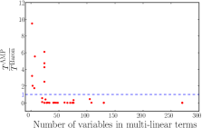
(a) AMP

(b) BT-AMP

Figure 11: Illustration of the ratio of run times of AMP and BT-AMP algorithms (with tuned parameters) to BARON. The y axis denotes the ratio and the x axis denotes the total number of variables in mutlilinear terms in a given MINLP instance. The blue dashed line indicates a ratio of 1. All red points correspond to a single instance. A point below the blue line indicates a ratio in favor of AMP.

4.5 OBBT Results for meyer15

One of the primary observations made in this paper is the importance of MIP-based sequential OBBT on medium-scale MINLPs. However, for a given large-scale MINLP, one of the drawbacks of BT and PBT is that it solves MILPs to tighten the variable bounds. Solving MILPs can be time consuming, in particular on instances like meyer15. Here, we focus on the run time issues associated with solving MILPs, suggest approaches for managing that run time and still get much of their benefits in bound-tightening.

Table 5 summarizes the run times of BT and PBT on meyer15 for various values of $\Delta$. As shown in the first row of this table, the run time varies drastically when the MILP is solved to optimality in every iteration of BT and PBT. To reduce this run time, we imposed a time limit on every $\min$- and $\max$-MILP of ten seconds. Since early termination of MILP does not guarantee optimal primal-feasible solutions, incumbent solutions are not valid for bound-tightening. Instead, we use the best lower bound maintained by the solver. This ensures the validity of the tightened bounds. As shown in the second row of Table 5, the run times of PBT are drastically reduced.

Table 6 summarizes the results of AMP based on the tightened variable bounds presented in Table 5. Interestingly, on meyer15, we observed that AMP converges to near optimal solutions (sometimes, even better than solving full MILPs) when the time limit on MILP solvers is imposed. This is an important feature for tuning the time spent tightening bounds vs bound solution quality. Further, this intriguing result suggests further study of MIP-based relaxations for OBBT of MINLPs, which we delegate for future work.

Table 5: BT and PBT run times on meyer15 with and without a limit on the run time of every MILP solved during the bound-tightening phase. Here, a 10-second time limit was used. The imposition of this limit reduces the total run time of PBT to close to BT.

	BT	PBT
		$\Delta=4$	$\Delta=8$	$\Delta=10$	$\Delta=16$	$\Delta=32$
Without time limit	3877	19218	32130	29586	11705	17868
With time limit	3830	3914	4059	4014	3635	3621

Table 6: AMP run times on meyer15 instance preceded by bound-tightening with (BT-lim, PBT-lim) and without limit (BT, PBT) on run time per iteration. Values under “Gap” and “$T$” are in % and seconds, respectively. Bold font represents the best result in each row.

	$\Delta=4$		$\Delta=8$		$\Delta=10$		$\Delta=16$		$\Delta=32$
	Gap	$T$	Gap	$T$	Gap	$T$	Gap	$T$	Gap	$T$
After BT	0.02	TO	0.08	TO	0.12	TO	0.31	TO	0.15	TO
After BT-lim	0.37	TO	0.14	TO	0.17	TO	0.69	TO	0.90	TO
After PBT	GOpt	536.56	GOpt	1600	GOpt	TO	0.20	TO	0.15	TO
After PBT-lim	0.37	TO	0.90	TO	0.19	TO	0.70	TO	0.90	TO

Table 7: Overall structure of the MINLP problems. The first column describes the name of the problem instance. The second column cites the source of the problem. The third column shows the optimal solution. The fourth, fifth and sixth columns show the number of constraints, binary variables, and continuous variables, respectively. The seventh column indicates the partitioned continuous variables. “ALL” refers to all variables in mutlilinear terms and “VC” refers to variables in the minimum vertex cover as described in boukouvala2016global . The final column shows the number of mutlilinear terms.

Instance	Ref.	GOpt	#Cons	#BVars	#CVars	#CVars-P	#ML
NLP1	nagarajan2016tightening	7049.248	14	0	8	ALL	5
fuel	bussieck2003minlplib	8566.119	15	3	12	VC	3
ex1223a	bussieck2003minlplib	4.580	9	4	3	VC	3
ex1264	bussieck2003minlplib	8.6	55	68	20	VC	16
ex1265	bussieck2003minlplib	10.3	74	100	30	VC	25
ex1266	bussieck2003minlplib	16.3	95	138	42	VC	36
eniplac	bussieck2003minlplib	-132117.083	189	24	117	VC	66
util	bussieck2003minlplib	999.578	167	28	117	ALL	5
meanvarx	bussieck2003minlplib	14.369	44	14	21	VC	28
blend029	bussieck2003minlplib	13.359	213	36	66	VC	28
blend531	bussieck2003minlplib	20.039	736	104	168	VC	146
blend146	bussieck2003minlplib	45.297	624	87	135	VC	104
blend718	bussieck2003minlplib	7.394	606	87	135	VC	100
blend480	bussieck2003minlplib	9.227	884	124	188	VC	152
blend721	bussieck2003minlplib	13.5268	627	87	135	VC	104
blend852	bussieck2003minlplib	53.9626	2412	120	184	VC	152
wtsM2_05	misener2013glomiqo	229.7008	152	0	134	VC	48
wtsM2_06	misener2013glomiqo	173.4784	152	0	134	VC	48
wtsM2_07	misener2013glomiqo	80.77892	152	0	134	VC	48
wtsM2_08	misener2013glomiqo	109.4014	335	0	279	VC	84
wtsM2_09	misener2013glomiqo	124.4421	573	0	517	ALL	210
wtsM2_10	misener2013glomiqo	586.68	138	0	156	VC	60
wtsM2_11	misener2013glomiqo	2127.115	252	0	304	VC	112
wtsM2_12	misener2013glomiqo	1201.038	408	0	517	VC	220
wtsM2_13	misener2013glomiqo	1564.958	783	0	1040	VC	480
wtsM2_14	misener2013glomiqo	513.009	205	0	209	VC	90
wtsM2_15	misener2013glomiqo	2446.429	152	0	134	VC	48
wtsM2_16	misener2013glomiqo	1358.663	234	0	244	VC	126
lee1	MINLP123	-4640.0824	82	9	40	VC	24
lee2	MINLP123	-3849.2654	92	9	44	VC	36
meyer4	MINLP123	1086187.137	118	55	63	VC	48
meyer10	MINLP123	1086187.137	423	187	207	VC	300
meyer15	MINLP123	943734.0215	768	352	382	VC	675

5 Conclusions

In this work, we developed an approach for adaptively partitioning nonconvex functions in MINLPs. We show that an adaptive partitioning of the domains of variables outperforms uniform partitioning, though the latter exhibits better optimality gaps in the first few iterations of the lower-bounding algorithm. We also show that bound-tightening techniques can be applied in conjunction with adaptive partitioning to improve convergence dramatically. We then use combinations of these techniques to develop an algorithm for solving MINLPs to global optimality. Our numerical experiments on MINLPs with polynomials suggests that this is a very strong approach with an advantage of having very few tuning parameters in contrast to the existing methods.

We have seen that using a well-designed MIP-based method with adaptive partitioning schemes is an attractive way of tackling MINLPs. With an apriori fixed tolerance, we get global optimum solutions by utilizing the well-developed state-of-the-art MIP solvers. However, though AMP is relatively faster than the available global solvers, we observed that the computation times remain large for MINLPs with large number of nonconvex terms, thus motivating a multitude of directions for further developments. First, it will be important to consider existing classical nonlinear programming techniques, such as dual-based bound-contraction, partition elimination within the branch-and-bound search tree, bound-tightening at sub nodes mouret2009tightening , and constraint propagation methods belotti2013bound , which can tremendously speed-up our algorithm. Second, providing apriori guarantees on the size of the added partitions ($\Delta$) that leads to faster tightening of the relaxations. This will support automatic tuning of $\Delta$ from within AMP. Third, recent developments on generating tight convex hull-reformulation-based cutting planes for solving convex generalized disjunctive programs will be very effective for attaining faster convergence to global optimum trespalacios2016cutting . Finally, extensions of our methods from polynomial to general nonconvex functions (including fractional exponents, transcendental functions and disjunctions of nonconvex functions) will be another direction that will have relevance to numerous practical applications.

Appendix A Appendix

A.1 Sensitivity Analysis of $\Delta$

One of the important details of MINLP algorithms and approaches is their parameterization. As seen in the earlier sections, AMP is no different. The quality of the solutions depend heavily on the choice of $\Delta$. However, in spite of this problem specific dependence, it is often interesting to identify reasonable default values. Table 8 presents computational results on all instances for different choices of $\Delta$. From these results, AMP is most effective when $\Delta$ is between 4 and 10.

Table 8: This table shows a sensitivity analysis of AMP’s performance to the choice of $\Delta$. Here, we bin results by $\Delta\leq 4$, $\Delta$ between 4 and 10, and $\Delta>10$. From these results, it is clear that most of the good choices of $\Delta$ are between 4 and 10 and this is our recommended choice for this parameter. For each instance, the bold face font represents best run time or the best optimality gap (if the solve times out)

	$\Delta\leq 4$		$4<\Delta\leq 10$		$\Delta>10$
Instances	Gap(%)	$T$	Gap(%)	$T$	Gap(%)	$T$
p1	GOpt	0.74	GOpt	0.24	GOpt	0.06
p2	GOpt	0.60	GOpt	0.20	GOpt	0.10
fuel	GOpt	0.05	GOpt	0.06	GOpt	0.07
ex1223a	GOpt	0.03	GOpt	0.02	GOpt	0.02
ex1264	GOpt	1.92	GOpt	0.79	GOpt	1.03
ex1265	GOpt	2.24	GOpt	0.28	GOpt	0.80
ex1266	GOpt	0.20	GOpt	0.23	GOpt	0.16
eniplac	GOpt	2.39	GOpt	1.46	GOpt	0.75
util	GOpt	2.52	GOpt	2.14	GOpt	0.55
meanvarx	GOpt	967.70	GOpt	118.80	GOpt	70.09
blend029	GOpt	1.98	GOpt	1.33	GOpt	1.00
blend531	GOpt	88.60	GOpt	74.33	GOpt	49.76
blend146	23.34	TO	1.60	TO	3.20	TO
blend718	GOpt	1263.41	GOpt	581.68	GOpt	889.72
blend480	0.10	TO	0.02	TO	0.02	TO
blend721	GOpt	486.17	GOpt	44.13	GOpt	176.11
blend852	0.01	TO	GOpt	144.26	GOpt	322.80
wtsM2_05	GOpt	2236.45	GOpt	2545.41	GOpt	386.95
wtsM2_06	0.02	TO	GOpt	519.38	GOpt	972.20
wtsM2_07	0.77	TO	0.57	TO	0.54	TO
wtsM2_08	7.92	TO	9.28	TO	11.96	TO
wtsM2_09	7.47	TO	68.58	TO	68.58	TO
wtsM2_10	0.11	TO	0.11	TO	0.10	TO
wtsM2_11	6.10	TO	6.27	TO	10.41	TO
wtsM2_12	6.49	TO	8.69	TO	4.00	TO
wtsM2_13	7.37	TO	2.03	TO	10.27	TO
wtsM2_14	4.06	TO	5.59	TO	1.43	TO
wtsM2_15	0.17	TO	0.17	TO	0.57	TO
wtsM2_16	5.73	TO	8.17	TO	5.25	TO
lee1	GOpt	73.19	GOpt	13.61	0.03	TO
lee2	0.38	TO	0.02	TO	0.08	TO
meyer4	GOpt	64.82	GOpt	5.33	GOpt	20.74
meyer10	GOpt	684.63	GOpt	133.47	9.70	TO
meyer15	0.10	TO	0.33	TO	0.15	TO
Summary	7		14		14

A.2 Logarithmic and Linear Encoding of Partition Variables

In section 2, the discussion on piecewise convex relaxations described formulations that encoded the partition variables with a linear number of variables and a logarithmic number of variables Vielma2009 . Table 9 compares the performance of AMP using both formulations. Despite fewer variables in the logarithmic formulation, this encoding is only effective on a few problems, generally on problems that require a significant number of partitions. These results suggest that when the logarithmic encoding has nearly the same number of partition variables as the linear encoding, the linear encoding is more effective.

Table 9: This table compares the logarithmic formulation of partition variables with the linear representation. Each column indicates the formulation with the fastest runtime for different choices of $\Delta$. The last column enumerates the number of times the logarithmic formulation is better.

Instances	$F(\Delta=4)$	$F(\Delta=8)$	$F(\Delta=10)$	$F(\Delta=16)$	$F(\Delta=32)$	Total
eniplac	lin	lin	log	log	log	3
blend531	lin	lin	log	lin	lin	1
blend146	lin	lin	log	lin	lin	1
blend718	lin	lin	lin	lin	log	1
blend480	lin	lin	log	lin	lin	1
blend721	lin	lin	lin	lin	lin	0
blend852	log	lin	log	lin	log	3
wtsM2_05	lin	lin	lin	lin	lin	0
wtsM2_06	lin	lin	lin	lin	lin	0
wtsM2_07	lin	lin	lin	lin	lin	0
wtsM2_08	log	lin	log	lin	log	3
wtsM2_09	lin	log	log	log	log	4
wtsM2_10	lin	lin	lin	lin	lin	0
wtsM2_11	lin	lin	lin	lin	lin	0
wtsM2_12	lin	lin	lin	lin	lin	0
wtsM2_13	lin	lin	lin	lin	lin	0
wtsM2_14	lin	lin	lin	lin	lin	0
wtsM2_15	log	lin	lin	log	lin	2
wtsM2_16	lin	lin	lin	lin	lin	0
lee1	log	log	log	log	log	5
lee2	log	lin	lin	lin	lin	1
meyer4	log	log	lin	lin	log	3
meyer10	lin	lin	log	log	lin	2
meyer15	log	log	lin	lin	log	3
${Total}$	7	4	9	5	8	33