Assouad dimension of random processes

Abstract.

In this paper we study the Assouad dimension of graphs of certain Lévy processes and functions defined by stochastic integrals. We do this by introducing a convenient condition which guarantees a graph to have full Assouad dimension and then show that graphs of our studied processes satisfy this condition.

1. Definitions and motivations

Studying the dimension of various random processes has been of interest for quite some time. In this paper we will consider the Assouad dimension of graphs of certain random processes, notably Lévy processes and functions defined by stochastic integrals.

Lévy processes $X(t)$ were first introduced by Paul Lévy in 1934 [Lév34] and are defined to be the stochastic processes satisfying:

• : $X(0)=0$ almost surely.

• : For all $t,h>0$, $X(t+h)-X(t)$ is equal to $X(h)$ in distribution (stationary increments).

• : For all $0<t_{1}<t_{2}<...<t_{k}$ the random variables $X(t_{i})-X(t_{i-1})$ are independent (independence of increments).

• : For all $t>0$ $\lim_{h\to 0}X(t+h)-X(t)=0$ in probability (continuity).

We can construct $X(t)$ such that it is almost surely right continuous with left limits (denoted càdlàg). Such processes are standard tools in many areas of modern mathematics and its applications. A common example of a Lévy process is the Wiener process (or Brownian motion) where property 2 (stationary increments) is replaced by Gaussian increments, so $X(t+h)-X(t)$ is normally distributed with mean 0 and variance $h$. One can similarly define $d$-dimensional Brownian motion by considering the vector-valued stochastic process $(W_{1},\ldots,W_{d})$ where the $W_{i}$ are independent Weiner processes.

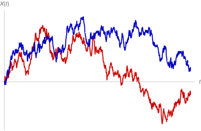
Figure 1. Two graphs of one-dimensional Brownian motion

The geometric properties, such as dimension, of Wiener processes have been a particularly well studied area. This includes studying the graphs, level sets and trails of such processes which can often be thought of as fractals as they often display some statistical self-affinity. For any left continuous function $X:\mathbb{R}\to\mathbb{R}$, we define the graph of the function by:

$$G^{I\subset\mathbb{R}}_{X}=\{(t,y)|y=X(t),t\in I\}\cup J,$$

where $J$ is the union of vertical segments joining the discontinuities. $J$ is well defined because $X$ is right continuous. It is clear that if $X$ is continuous then $J$ is empty. Taylor [Tay53] first calculated the Hausdorff dimension of $d$-dimensional Brownian motion $B_{d}:\mathbb{R}\to\mathbb{R}^{d}$ where he showed that almost surely

$$\dim_{\text{H}}G_{B_{1}}^{[0,1]}=\frac{3}{2}$$

and for any $d\geq 2$

$$\dim_{\text{H}}B_{d}([0,1])=2.$$

Another generalisation of Brownian motion is fractional Brownian motion, first introduced by Mandelbrot and Van Ness [MV68]. Index-$h$ fractional Brownian motion (fBm) on $\mathbb{R}$ with $0<h<1$ is defined to be the stochastic integral

$$B_{h}(t)=c(h)^{-1}\int_{-\infty}^{\infty}\left(\left(t-x\right)_{+}^{h-1/2}-(-x)_{+}^{h-1/2}\right)W(dx)$$

where W is the Wiener measure, $(x)_{+}=\max\{0,x\}$ and $c(h)=\Gamma(h+1/2)$, where $\Gamma$ denotes the gamma function. Equivalently this is a Gaussian random process $B_{h}(t)$ with:

• : $B_{h}(0)=0$ almost surely.

• : For all $t,u>0$, $B_{h}(t+u)-B_{h}(t)$ has normal distribution with mean 0 and variance $u^{2h}$ (Gaussian increments).

• : For all $t>0$ $\lim_{u\to 0}B_{h}(t+u)-B_{h}(t)=0$ in probability (continuity).

One can see that when $h=1/2$, $B_{1/2}(t)=B(t)$ is simply Brownian motion. Much progress has been made on the properties of fBm, see for instance [Adl77],[Kah85] and [Fal15]. Notably it was shown that almost surely, the graph over the unit interval of index-$h$ fBm has Hausdorff dimension $2-h$.

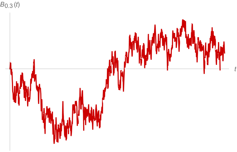
(a) Graph of fBm with h=0.3

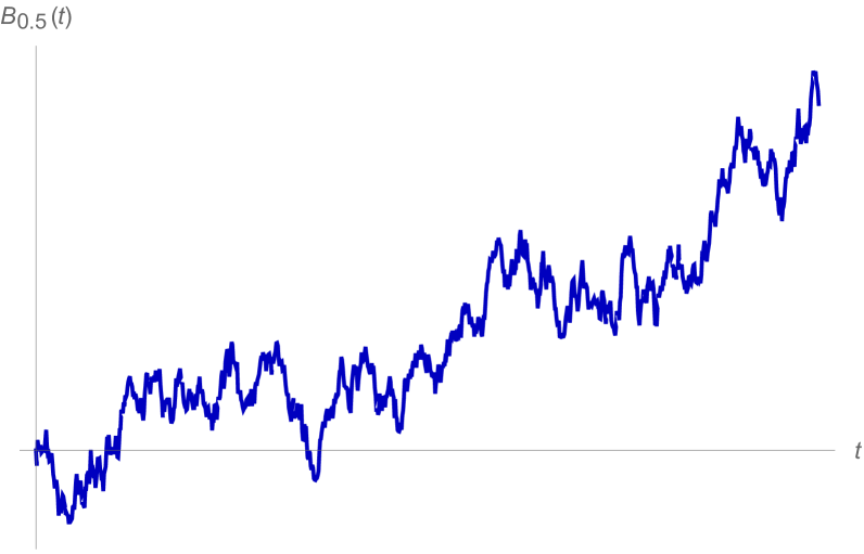
(b) Graph of fBm with h=0.5

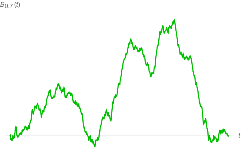
(c) Graph of fBm with h=0.7

Studying the Assouad dimension of various fractals and its properties is an increasingly popular area of research. In this paper, we are interested in calculating the Assouad dimension of the graph $G_{X}^{[0,1]}$ for $\beta$-scaling (or Lévy $\beta$-stable) processes and stochastic integrals $X$. These results will be compared to the previously obtained Hausdorff dimensions.

We say that $X(t)$ satisfies a $\beta$-scaling property if, for any $t,a>0$:

$$a^{-\frac{1}{\beta}}X(at)=^{d}X(t),$$

where ‘$=^{d}$’ denotes ‘equal in distribution’. For example the Wiener process has the $2$-scaling property.

A non-empty compact bounded set $F$ is said to be $s$-homogeneous if there exists a constant $C>0$ such that for all $0<R$, $r\in(0,R]$ and $x\in F$

$$N(B(x,R)\cap F,r)\leq C\left(\frac{R}{r}\right)^{s}$$

where $B(x,R)$ denotes the closed ball of centre $x$ and radius $R$ and $N(E,r)$ is the number of squares of the $r\times r$ grid that intersect the compact set $E$.

The Assouad dimension of a non-empty compact bounded set $F$ is then defined to be

$$\dim_{\mathrm{A}}F=\inf\left\{s\geq 0\,\,\colon\,F\text{ is }s\text{-homogeneous}\right\}.$$

This dimension provides information on the extremal local scaling of a set, in this setting it will tell us about the maximal fluctuations of a random process. For a more detailed introduction to this dimension, see [Fra14, Rob11].

This paper will be split into three parts. First we will define a condition, Definition 2.1 which guarantees that a graph will have full Assouad dimension. Then in Section 3 we show that graphs of $\beta$-scaling Lévy process satisfy this condition and combining these results we prove that graphs of functions defined by certain stochastic integrals also have full Assouad dimension. Finally in Section 4 we remark that our results extend to higher dimensions.

2. Assouad dimension of graphs

In this section we will state a convenient condition to check whether a graph of a function $f:[0,1]\to\mathbb{R}$ has full Assouad dimension.

We begin with a definition:

Definition 2.1.

Let $R_{1},R_{2}>0$ be positive numbers and $n_{1},n_{2}>0$ be integers. Given a point $a\in\mathbb{R}^{2}$, we define $W_{n_{1}\times n_{2}}^{R_{1}\times R_{2}}(a)$ as the following collection of sets:

$$\left\{D_{i,j}+a\,|\,D_{i,j}=\left[\frac{i}{n_{1}}R_{1},\frac{i+1}{n_{1}}R_{1}\right]\times\left[\frac{j}{n_{2}}R_{2},\frac{j+1}{n_{2}}R_{2}\right],i\in\{0,\dots,n_{1}-1\},j\in\{0,\dots,n_{2}-1\}\right\}.$$

We see that $W_{n_{1}\times n_{2}}^{R_{1}\times R_{2}}(a)$ is the collection of rectangles with disjoint interiors which partitions the $R_{1}\times R_{2}$ rectangle whose bottom left vertex is $a$.

Then let $N_{n_{1}\times n_{2}}^{R_{1}\times R_{2}}(a,G_{f}^{[0,1]})=\#\left\{W_{n_{1}\times n_{2}}^{R_{1}\times R_{2}}(a)\cap G_{f}^{[0,1]}\right\}$, this is the number of rectangles which intersect the graph.

The following theorem is a direct consequence of the definition of Assouad dimension and we omit the proof:

Theorem 2.2.

If there exists an $A>0$ and sequences:

$$a_{i}\in\mathbb{R}^{2},R_{i}\in(0,1),\,n_{i}\in\mathbb{N}\quad(\forall i\in\mathbb{N})$$

with $n_{i}\rightarrow\infty$ such that for all $i\in\mathbb{N}$

$$N_{n_{i}\times n_{i}}^{R_{i}\times R_{i}}(a_{i},G_{f}^{[0,1]})\geq An_{i}^{2}.$$

Then

$$\dim_{\mathrm{A}}G_{f}^{[0,1]}=2.$$

Whilst this might seem like a restrictive condition to ask a general function to satisfy, it is quite natural in the setting of Wiener processes due to the almost sure unbounded variation and $\beta$-scaling property of the process. Considering squares instead of balls in the definition of Assouad dimension is similar to the definition of the Furstenberg star dimension, which is in fact equivalent to the Assouad dimenion, see [CWW16].

Remark 2.3.

Note that one could replace the inequality with the following equality

$$N_{n_{i}\times n_{i}}^{R_{i}\times R_{i}}(a_{i},G_{f}^{[0,1]})=n_{i}^{2}.$$

This follows from [FY16, Theorem 2.4], where it is shown that a set has full Assouad dimension if and only if it has the unit ball as a weak tangent. This means that any cover of our set is also a cover of a ball and so all smaller squares are needed in the cover.

3. Applications to $\beta$-scaling Lévy processes

Let $X(t)$ be a Lévy process. We assume that $X(1)$ is non-vanishing almost everywhere on $\mathbb{R}$ as a random variable, that is, the distribution function of $X(1)$ is 0 only on a set of measure 0.

Then for any $\beta$-scaling Lévy process $X$ we can compute the probability of the following event ‘$N_{n\times n}^{1\times 1}(0,G_{X}^{[0,1]})=n^{2}$’. It is a positive number depending only on $n$ and we use $P(n)$ to denote this number. The event ‘$X$ hits a rectangle’ is measurable when $X$ is continuous; when it is discontinuous we join the graph with a vertical line and the process is càdlàg so the event ‘$X$ hits a rectangle’ is still measurable. Thus our event is measurable as the union of measurable events.

For a $\beta$-scaling random process $X$, we can decompose the graph into countably many disjoint parts:

$$G_{X}^{[0,1]}=\bigcup_{i=0}^{\infty}G_{X}^{I_{i}},$$

where $I_{i}$ are closed intervals with disjoint interiors such that their union is the unit interval. For our case one could think of this as partitioning the unit interval by intervals of length $1/2^{i}$. For example take $a_{1}=0$ and for all $i\geq 1$ let $a_{i+1}=a_{i}+1/2^{i}$ and $I_{i}=[a_{i},a_{i}+1/2^{i}].$

Denote by $|I_{i}|$ the length of interval $I_{i}=[a_{i},b_{i}]$. Because we can take $X$ as a left continuous function, $X(a_{i})\in\mathbb{R}$ is defined for all $i$. For each $i$ we can apply a linear map $T_{i}:G_{X}^{I_{i}}\rightarrow[0,1]^{2}$:

$$T_{i}(x,y)=\left(\frac{1}{|I_{i}|}(x-a_{i}),\frac{1}{|I_{i}|^{1/\beta}}(y-X(a_{i}))\right).$$

By definition, it is easy to see that $T_{i}(G_{X}^{I_{i}})$ are independent $\beta$-scaling Lévy processes with the same, original distribution. For convenience we identify $T_{i}(G_{X}^{I_{i}})=G_{X_{i}}^{[0,1]}$ where $X_{i}$ are independent, identically distributed $\beta$-scaling Lévy processes.

Let $n_{i}$ be a sequence of integers such that $\lim_{i\to\infty}n_{i}=\infty$. We can compute the probability of the event $A_{i}=`N_{n_{i}\times n_{i}}^{1\times 1}((0,0),G_{X_{i}}^{[0,1]})=n_{i}^{2}$’. According to the discussions above, we see that the probability is $P(n_{i})$. In fact denote $t_{k}=k/n^{2}_{i}$ for all $k\in\{1,\dots,n^{2}_{i}\}$ and $D(j)=[j/n_{i},(j+1)/n_{i}]$ for all $j\in\{0,\dots,n_{i}-1\}$ then we can see that:

$$P(n_{i})\geq P\left(\forall k\in\left[1,n^{2}_{i}\right],k\in\mathbb{N},X(t_{k})\in D\left(\left\{\frac{k}{n_{i}}\right\}n_{i}\right)\right)>0.$$

Here $\{\cdot\}$ denotes the fractional part function. The last inequality follows from our assumption that $X(1)$ is non-vanishing almost everywhere on $\mathbb{R}$. It is clear that this restraint could be relaxed to non-vanishing on some interval without much effort. The rest follows from the property of independent increments.

We can choose $n_{i}$ to grow slowly enough such that $\sum_{i}P(n_{i})=\infty$. Note that the $R_{i}$ can be chosen so that each square is disjoint and as Lévy processes are Markov, the events $A_{i}$ are all independent. Then by Borel-Cantelli lemma we see that with probability $1$, infinitely many events $A_{i}$ occur. Now if $A_{i}$ happens, then:

$$N_{n_{i}\times n_{i}}^{1\times 1}\left((0,0),G_{X_{i}}^{[0,1]}\right)=n_{i}^{2},$$

applying the function $T^{-1}_{i}$ to the graph, we see that (remember $I_{i}=[a_{i},b_{i}]$):

$$N_{n_{i}\times n_{i}}^{|I_{i}|\times|I_{i}|^{1/\beta}}\left((a_{i},X(a_{i})),G_{X}^{I_{i}}\right)=n_{i}^{2}.$$

Since $\beta\geq 1$, we see that $|I_{i}|\leq|I_{i}|^{1/\beta}$. Also remember that $X$ can be taken to be a right continuous function and we also include the vertical segments of the jumps in $G^{[0,1]}_{X}$. Therefore it is clear that there exist an absolute constant $C>0$:

$$N\left(B\left(\left(a_{i},X(a_{i})\right),|I_{i}|\right)\cap G_{X}^{[0,1]},\frac{|I_{i}|}{n_{i}}\right)\geq Cn_{i}^{2}.$$

As infinitely many $A_{i}$ occur, using Theorem 2.2, we see:

$$\dim_{\mathrm{A}}G_{X}^{[0,1]}=2.$$

We conclude the above argument as the following theorem:

Theorem 3.1.

Let $X$ be a $\beta$-scaling Lévy process with $\beta\geq 1$, such that $X(1)$ is a random variable whose distribution function is non-vanishing almost everywhere. Then almost surely:

$$\dim_{\mathrm{A}}G_{X}^{[0,1]}=2.$$

We know that the Wiener process $W(t)$ is a $2$-scaling Lévy process, therefore we see that:

Corollary 3.2.

$$\dim_{\mathrm{A}}G_{W}^{[0,1]}=2.$$

Ville Suomala and Changhao Chen, in a personal communication, kindly remarked that this result follows from the graph of Brownian motion having full lower porosity dimension. This approach is inspired by [CG91], where it was shown that the graph of Brownian motion has full upper porosity dimension. However this porosity dimension technique does not extend to our following, more general result, which relies upon this one.

In fact we can say more about the Assouad dimension of random processes which are functions defined as stochastic integrals, such as fractal Brownian motion.

Theorem 3.3.

Let $f:\mathbb{R}\to\mathbb{R}$ be a function which is zero only finitely often, continuous on some interval and has continuous derivative on that same interval. Then we define $B_{f}(t)$ as the function defined by the stochastic integral:

$$B_{f}(t)=\int_{0}^{t}f(x)W(dx).$$

We have that almost surely:

$$\dim_{\mathrm{A}}G_{B_{f}}^{[0,1]}=2.$$

Remark 3.4.

In particular, graphs of fractional Brownian motions with indices $0<h<1$ have full Assouad dimension almost surely.

Proof.

Given a function $f$ which is zero only finitely often, continuous and has continuous derivative on some interval, say $J$, we can simply focus on the function restricted to $J$, normalising to obtain a function which is $C^{1}$ and zero only finitely often on the unit interval. We may then assume that $f(t)>1$ for $t\in[0,1]$ by again restricting our function to an interval where the function is bounded away from zero and normalising.

As the Assouad dimension provides local information, if the dimension of the graph of the function defined by stochastic integral of this new function is full then the dimension of the original graph is also full. Thus we assume for the rest of this proof that $f$ is a $C^{1}$ function which is greater than $1$.

Ideally we would wish to integrate by parts in the standard Riemann–-Stieltjes sense

$$\int_{0}^{t}f(x)W(dx)=f(t)W(t)-\int_{0}^{t}W(x)f^{\prime}(x)dx.$$

The problem is that the integral on the left side of the above equation is interpreted as the Itô integral, for which regular integration by parts does not hold. There is however a generalisation of this formula for stochastic integrals which holds as $f$ and $W$ are both semimartingales, see [Pro05][Chapter 2 Section 6] for further details. To be precise we should write the following equation

$$\int_{0}^{t}f(x)W(dx)=f(t)W(t)-\int_{0}^{t}W(x)f^{\prime}(x)dx-[f,W]_{t}.$$

Here $[f,W]_{t}$ is the quadratic covariation between $f$ and $W$:

Let $0=t_{1}<t_{2}<\dots<t_{n}=t$ be a partition $P$ of $[0,t]$ and $|P|$ be the maximum of $t_{k+1}-t_{k},k\in\{0,\dots,n-1\}$:

$$[f,W]_{t}=\lim_{|P|\to 0}\sum_{i=1}^{n-1}(f(t_{i+1})-f(t_{i}))(W(t_{i+1})-W(t_{i})).$$

The above convergence is taken in the sense of probability. By using Cauchy-Schwarz we see that:

$$[f,W]_{t}\leq[f,f]^{1/2}_{t}[W,W]^{1/2}_{t}.$$

However, it is standard that $[f,f]_{t}=0$ and $[W,W]_{t}=t$ as $f$ is $C^{1}$. So we see that the integral by parts formula (*) is indeed correct for this situation. The integral

$$\int_{0}^{t}W(x)f^{\prime}(x)dx$$

is defined to be a random process whose sample space is that of the Wiener process, where fixing a sample path of the Wiener process will determine the integral. We are interested in almost sure properties of this process and will do so by considering almost sure properties of the Wiener process.

The strategy for the rest of this proof is to choose carefully a typical path of the Wiener process. We denote the sample space of the Wiener process as $\Omega$.

First, we see that for almost all $\omega\in\Omega$, $W(t,\omega)$ is càdlàg in $t$, and therefore there is a constant $C_{\omega}$ such that:

$$|W(t,\omega)|\leq C_{\omega}$$

for all $t\in[0,1]$.

The second almost sure property is described in the proof of Theorem 3.1, that there are infinitely many intervals $I_{i}=[a_{i},b_{i}]\subset[0,1]$ and a sequence $n_{i}\to\infty$ such that for $k\in\{0,1,\dots,n_{i}-1\}$

$$\left|W\left(a_{i}+(k+1)\frac{|I_{i}|}{n_{i}},\omega\right)-W\left(a_{i}+k\frac{|I_{i}|}{n_{i}},\omega\right)\right|\geq|I_{i}|^{1/2}\geq|I_{i}|.$$

In the following discussion we shall fix a typical $\omega$ such that $W(t,\omega)$ satisfies the above two almost sure properties, in particular, we think of $C_{\omega}>0$ as a fixed constant.

Then we see that:

$$\left|B_{f}\left(a_{i}+(k+1)\frac{|I_{i}|}{n_{i}},\omega\right)-B_{f}\left(a_{i}+k\frac{|I_{i}|}{n_{i}},\omega\right)\right|$$

$$= \left|\int_{a_{i}+k\frac{|I_{i}|}{n_{i}}}^{a_{i}+(k+1)\frac{|I_{i}|}{n_{i}}}f(x)W(dx)\right|$$

$$= \left|f\left(a_{i}+k\frac{|I_{i}|}{n_{i}}\right)W(x,\omega)\bigg{|}_{a_{i}+k\frac{|I_{i}|}{n_{i}}}^{a_{i}+(k+1)\frac{|I_{i}|}{n_{i}}}+\int_{a_{i}+k\frac{|I_{i}|}{n_{i}}}^{a_{i}+(k+1)\frac{|I_{i}|}{n_{i}}}W(x)f^{\prime}(x)dx\right|.$$

Since $f$ is $C^{1}$, we see that there is a constant $C_{f}$ (which does not depend on $i$) such that for all $x\in\left[{a_{i}+k\frac{|I_{i}|}{n_{i}}},{a_{i}+(k+1)\frac{|I_{i}|}{n_{i}}}\right]$:

$$\left|W(x)f^{\prime}(x)\right|\leq C_{f}C_{\omega}.$$

Then we have the following inequalities:

$$\left|f\left(a_{i}+k\frac{|I_{i}|}{n_{i}}\right)W(x,\omega)\bigg{|}_{a_{i}+k\frac{|I_{i}|}{n_{i}}}^{a_{i}+(k+1)\frac{|I_{i}|}{n_{i}}}\right|\geq\left|f\left(a_{i}+k\frac{|I_{i}|}{n_{i}}\right)\right||I_{i}|^{1/2}\geq|I_{i}|^{1/2}.$$

and

$$\left|\int_{a_{i}+k\frac{|I_{i}|}{n_{i}}}^{a_{i}+(k+1)\frac{|I_{i}|}{n_{i}}}W(x)f^{\prime}(x)dx\right|\leq C_{f}C_{\omega}\frac{|I_{i}|}{n_{i}}.$$

Since $|I_{i}|\to 0$, we see that for a constant $C^{\prime}$ which depends only on $f$ and $\omega$:

$$\left|B_{f}\left(a_{i}+(k+1)\frac{|I_{i}|}{n_{i}},\omega\right)-B_{f}\left(a_{i}+k\frac{|I_{i}|}{n_{i}},\omega\right)\right|\geq C^{\prime}|I_{i}|.$$

The above inequality holds for all $k\in\{0,\dots,n_{i}-1\}$.

Moreover, $W$ has a ‘zigzag’ property. For even integers $k$ we have

$$W\left(a_{i}+(k+1)\frac{|I_{i}|}{n_{i}},\omega\right)-W\left(a_{i}+k\frac{|I_{i}|}{n_{i}},\omega\right)>0,$$

for odd integers $k$ we have

$$W\left(a_{i}+(k+1)\frac{|I_{i}|}{n_{i}},\omega\right)-W\left(a_{i}+k\frac{|I_{i}|}{n_{i}},\omega\right)<0.$$

Heuristically this says that the process increases on the first interval, decreases on the second and so forth, zigzagging from top to bottom. We can see that the expressions inside the absolute values in (**) and (***) also satisfy similar ‘zigzag’ properties. Therefore there is a constant $A=A(\omega,f)>0$ such that:

$$N\left(B\left(\left(a_{i},B_{f}(a_{i})\right),|I_{i}|\right)\cap G_{B_{f}}^{[0,1]},\frac{|I_{i}|}{n_{i}}\right)\geq An_{i}^{2}.$$

This concludes the proof because the above argument holds for a set of full probability $\omega\in\Omega$. ∎

4. A remark on higher dimensional Brownian motion

Definition 2.1 has a natural generalization in $\mathbb{R}^{d}$.

Definition 4.1.

Let $R_{1},\dots,R_{d}>0$ be positive numbers and $n_{1},\dots,n_{d}$ be integers. Given a point $a\in\mathbb{R}^{d}$, we define $W_{n_{1}\times\dots\times n_{d}}^{R_{1}\times\dots\times R_{d}}(a)$ as the following collection of sets:

$$\Bigg{\{}D_{i_{1},\dots,i_{d}}+a\,|\,D_{i_{1},\dots,i_{d}}=\left[\frac{i_{1}}{n_{1}}R_{1},\frac{i_{1}+1}{n_{1}}R_{1}\right]\times\dots\times\left[\frac{i_{d}}{n_{d}}R_{d},\frac{i_{d}+1}{n_{d}}R_{d}\right],$$

$$i_{j}\in\{0,\dots,n_{j}-1\},j\in\{1,\dots,d\}\Bigg{\}}.$$

We see that $W_{n_{1}\times n_{2}}^{R_{1}\times R_{2}}(a)$ is a collection of rectangles with disjoint interiors.

Using the above definition and a similar argument as the one in section 3, Theorem 2.2 also extends to higher dimensions, we can show the following result and we omit the proof:

Theorem 4.2.

Let $B_{d}(t)$ be the $d$ dimensional Brownian motion, from $\mathbb{R}$ to $\mathbb{R}^{d}$. Then almost surely:

$$\dim_{\mathrm{A}}B_{d}([0,1])=d.$$

We can compare this result to the well known

$$\dim_{\mathrm{H}}B_{d}([0,1])=2$$

for $d\geq 2$. The Hausdorff dimension being 2 here can be thought as a reflection that higher dimensional Brownian motion is transient, whilst the Assouad dimension shows that there are still areas of maximal fluctuation.

Brownian motion also provides examples of Salem sets that can have different Hausdorff and Assouad dimensions, we refer the reader to [Kah85] for further discussion on the links between random processes and Salem sets.

Acknowledgements

DCH was financially supported by EPSRC Doctoral Training Grant EP/N509759/1. HY thanks the University of St Andrews’ School of Mathematics and Statistics for the PhD scholarship.

References

- [Adl77] R.J. Adler, Hausdorff dimension and Gaussian fields, Annals of Probability 5 (1977), 145–151.
- [CWW16] C. Chen, M. Wu and W. Wu, Accessible values of Assouad and the lower dimensions of subsets, preprint, (2016), available at: https://arxiv.org/abs/1602.02180.
- [CG91] J.T. Cox and P.S. Griffin, How porous is the graph of Brownian motion, Trans. Amer. Math. Soc. 325, (1991), no. 1, 119–140.
- [Fal15] K. Falconer, From fractional Brownian motion to multifractional and multistable motion, in M Frame & N Cohen (eds), Benoit Mandelbrot - A Life in Many Dimensions. World Scientific Publishing, 4 (2015).
- [Fra14] J.M. Fraser, Assouad type dimensions and homogeneity of fractals, Transactions of the American Mathematical Society 366 (2014), 6687–6733.
- [FY16] J. M. Fraser and H. Yu. Arithmetic patches, weak tangents, and dimension, preprint, (2016), available at: http://arxiv.org/abs/1611.06960.
- [Kah85] J.-P. Kahane, Some random series of functions, 2 ed., Cambridge Studies in Advanced Mathematics, Cambridge University Press, 1985.
- [Lév34] P. Lévy, Sur les intégrales dont les éléments sont des variables aléatoires indépendentes, Annali della Scuola Normale Superiore di Pisa 3 (1934), 337–366.
- [MV68] B.B. Mandelbrot and J. VanNess, Fractional Brownian motions, fractional noises and applications, SIAM review 10 (1968), no. 4, 422–437.
- [MP10] P. Möters and Y. Peres, Brownian Motion, Cambridge series in statistical and probabilistic mathematics, (2010)
- [Pro05] P. Protter, Stochastic Integration and Differential Equations, 2 ed., Stochastic Modelling and Applied Probability, Springer-Verlag Berlin Heidelberg, 2005
- [Rob11] J.C. Robinson, Dimensions, embeddings and attractors, Cambridge University Press, Cambridge, 2011.
- [Tay53] S.J. Taylor, The Hausdorff -dimensional measure of Brownian paths in -space, Mathematical Proceedings of the Cambridge Philosophical Society 49 (1953), no. 2, 31–39.