Galois groups in a family of dynatomic polynomials
Abstract.
For every nonconstant polynomial , let denote the fourth dynatomic polynomial of . We determine here the structure of the Galois group and the degrees of the irreducible factors of for every quadratic polynomial . As an application we prove new results related to a uniform boundedness conjecture of Morton and Silverman. In particular we show that if is a quadratic polynomial, then, for more than of all primes , does not have a point of period four in .
1. Introduction
Let be a nonconstant polynomial. For every positive integer , let denote the -fold composition of with itself. An algebraic number is called periodic under iteration of if there exists such that ; in that case the least such is called the period of .
A fundamental conjecture of Morton and Silverman [25] would imply that as varies over all polynomials of fixed degree , the possible periods of rational numbers under iteration of remain bounded. In [28] Poonen studied the case and conjectured that no quadratic polynomial over has a rational point of period greater than 3.
A useful construction for studying these conjectures is that of a dynatomic polynomial. For every nonconstant polynomial and every positive integer , the dynatomic polynomial of is defined by the equation
| (1.1) |
where is the Möbius function. The key property that motivates this definition is that the roots of are precisely the algebraic numbers having period under iteration of , except in rare cases when some roots may have period smaller than ; see [24, Thm. 2.4] for further details. By studying algebraic properties of the dynatomic polynomials of one may thus hope to gain information about the dynamical properties of as a map . With this in mind, let us now focus on the case of quadratic polynomials and discuss the following problem, which we consider to be especially important for understanding the dynamics of such maps.
Problem 1.1.
Given , determine all possible groups that can arise as the Galois group of for some quadratic polynomial . Furthermore, determine all possible factorization types111By the factorization type of a polynomial we mean the multiset of degrees of irreducible factors of . of that can arise as varies over all quadratic polynomials.
This problem is easily solved for and 2. The case is substantially harder, but was solved by Morton [22]. The purpose of this article is to treat the case . At present there appears to be no published work concerning the structure of the Galois groups of the polynomials in this case. Regarding factorization types we are only aware of two results in the literature: Morton [23, Thm. 4] showed that can never have a factor of degree 1, and Panraksa [27, Thm. 2.3.5] showed that cannot have four or more irreducible quadratic factors.
In order to state our results for we introduce some notation. For every quadratic polynomial there exist a unique rational number and a unique linear polynomial such that
The polynomials and share all the properties we are concerned with in this article; in particular, their dynatomic polynomials factor in the same way and have the same Galois group (see [15, §2.2]). In stating our results we may therefore restrict attention to the family of polynomials . To ease notation we will write instead of .
Let be the rational functions defined by
| (1.2) |
The set of all numbers of the form with will be denoted by . Similarly, we define sets and . We can now state our main result.
Theorem 1.2.
Let . Let and , respectively, denote the Galois group and factorization type of . Referring to the groups , and defined in Appendix A, we have the following:
-
(1)
If and , then and .
-
(2)
If , then and .
-
(3)
Suppose that . Then the following hold:
-
(a)
If , then and .
-
(b)
If , then and .
-
(a)
For the numbers excluded in the above theorem, the factorization types and isomorphism types of are given in Table 1.
In addition to solving Problem 1.1 for , Theorem 1.2 provides a way to improve on earlier results. As mentioned above, Morton showed that there is no such that has a rational point of period 4. We can obtain this theorem as a consequence of Theorem 1.2, as it is simply the observation that . Morton’s theorem was strengthened by the author in [15], where it is shown that for every quadratic polynomial there exist infinitely many primes such that does not have a point of period four in . By using the information about Galois groups afforded by Theorem 1.2, we can now prove the following stronger statement.
Theorem 1.3.
Let be a quadratic polynomial. Then, for more than of all primes (in the sense of Dirichlet density), does not have a point of period four in .
This article is organized as follows. In §2 we review the necessary background material on dynatomic polynomials. In §3 we develop the main tools used in the proof of Theorem 1.2. In §4 we prove this theorem and then deduce Theorem 1.3. Finally, in §5 we determine the rational points on a number of hyperelliptic curves that arise at various stages of the proof.
2. Dynatomic polynomials
Let be a field of characteristic and let be a nonconstant polynomial. For every positive integer , the dynatomic polynomial of is defined by the formula (1.1).
Two special cases of this definition are especially relevant here. First, the case where and is a polynomial of the form . In this case the polynomial will be denoted . Second, the case where is the rational function field and . In this case the polynomial will be denoted . By a basic property of dynatomic polynomials (see [24, Thm. 3.1]), for every the specialization is equal to the dynatomic polynomial of . Hence .
The Galois group and factorization type of the polynomial are well understood. Indeed, Bousch [4, Chap. 3] showed that is irreducible in and determined its Galois group over . It follows from Bousch’s results that is irreducible in and its Galois group over is isomorphic to the wreath product of with the symmetric group , where . Thus, the problem of classifying the Galois groups and factorization types of the polynomials for can be regarded as a special case of the following more general problem.
Problem 2.1.
Given a polynomial with known Galois group and factorization type, determine the Galois group and factorization type of every specialization with .
In the next section we discuss a technique that can be used to solve this problem under certain assumptions on the polynomial .
3. Explicit Hilbert Irreducibility
Let be a polynomial of degree in the variable . Regarding as an element of the ring , let be its leading coefficient, its discriminant, and its factorization type, i.e., the multiset of degrees (in ) of the irreducible factors of . Let be a splitting field for and let be the Galois group of .
For every rational number we let and we denote by and , respectively, the Galois group and factorization type of . By Hilbert’s Irreducibility Theorem [30, Prop. 3.3.5], for every number outside of a thin subset of we have and . We define the exceptional set of , denoted , to be the set of rational numbers for which either one of these conditions fails:
The purpose of this section is to develop a technique that can be used to explicitly describe the set and to determine and for every , especially in the case where is irreducible. For a more general treatment of this subject we refer the reader to the article [17].
Let be the ring and let be the integral closure of in . If is a maximal ideal of (henceforth referred to as a prime of ), we denote by the decomposition group of over .
For all satisfying , let be the kernel of the evaluation homomorphism given by .
Throughout this paper we will use the following notation to distinguish between an isomorphism of groups and an isomorphism of groups with an action.
Notation 3.1 (Isomorphism of group actions).
Suppose that the groups and act on sets and , respectively. We write if there exist an isomorphism and a bijection such that for all and all .
Lemma 3.2.
Suppose that satisfies . Then the following hold:
-
(1)
Let be a prime of dividing . Then , where acts on the roots of and acts on the roots of .
-
(2)
If , then .
Proof.
Statement (1) is well known, at least in the case where is monic and irreducible; a proof can be found in [18, Chap. VII, Thm. 2.9]. We include a sketch of the general case here.
For every element let denote the reduction of modulo . The extension of residue fields is Galois, and there is a surjective homomorphism given by , where
| (3.1) |
The condition implies that is unramified in , so this map is in fact an isomorphism. If denote the roots of in , then are the roots of in . Moreover, one can show that
so that is a splitting field for and hence . We therefore have an isomorphism and a bijection between the set of roots of and the set of roots of . The property (3.1) then implies that , proving (1).
Suppose now that . To prove (2) we will show that for every irreducible factor of , the polynomial remains irreducible; the result then follows immediately.
Let be an irreducible factor of and let be a prime of dividing . By (1) we have . Since and , we must have and therefore . The proof of (1) provides an isomorphism and a bijection between the roots of and the roots of . The map is the restriction of a ring homomorphism, so the roots of are mapped bijectively by to the roots of . Thus it is still the case that if we regard as acting on the roots of and as acting on the roots of . Since acts transitively on the roots of , must act transitively on the roots of . Hence is irreducible, as claimed. ∎
The following two propositions will be our main tools for describing the exceptional set of and determining the Galois group of every exceptional specialization .
Proposition 3.3.
Let be a subgroup of and let be a monic irreducible polynomial in such that the fixed field of is generated over by a root of . Suppose that satisfies
Then the following are equivalent:
-
(1)
The polynomial has a rational root.
-
(2)
There exists a prime of dividing such that .
Proof.
Let be the fixed field of and let be a root of such that . Let be the integral closure of in . The condition implies that is relatively prime to the conductor of the ring in . The Dedekind-Kummer theorem [26, p. 47, Prop. 8.3] therefore allows us to relate the factorization of the polynomial to the factorization of in . In particular, the theorem implies that has a rational root if and only if there exists a prime of dividing such that the residue degree of over is equal to 1. Since is unramified over , a maximality property of decomposition fields (see [20, p. 118, Prop. 8.6]) implies that (1) occurs if and only if there exists a prime of dividing such that is contained in the fixed field of . This proves the proposition, since the latter condition is clearly equivalent to (2). ∎
Proposition 3.4.
Let be representatives of all the conjugacy classes of maximal subgroups of . For let be the fixed field of and let be a monic irreducible polynomial such that the extension is generated by a root of . Suppose that satisfies
Then if and only if there is an index such that has a rational root.
Proof.
Remark 3.5 (Algorithmic aspects).
Propositions 3.3 and 3.4 can be used in practice to explicitly describe the exceptional set of and to determine the structure of the Galois group for every . It is crucial for these purposes to be able to compute the Galois group as well as a defining polynomial for the fixed field of any subgroup of . Both of these tasks can be carried out using known methods. Indeed, an algorithm of Fieker and Klüners [11] can be used to compute , and then the fixed field of any subgroup of can be computed as described in [14, §3.3], for instance. In the case where is irreducible, these methods were implemented by Fieker and are available via the Magma [3] functions GaloisGroup and GaloisSubgroup. The general case where is allowed to be reducible is treated in the article [17]; however we will not be needing here the algorithms for that case.
We end this section with a proposition that can be used to determine the factorization types for all when the set is a finite union of infinite sets, each of which can be parametrized by a rational function. As will be shown in Proposition 4.8, this is the case for the exceptional set of the dynatomic polynomial .
Proposition 3.6.
Suppose that is a rational function such that the polynomial is monic and irreducible and has a root . Let and . Then the following hold:
-
(1)
Suppose that satisfies and has the form for some . Then there exists a prime of dividing such that .
-
(2)
Define a polynomial , where is chosen so that has coefficients in . Then .
-
(3)
With notation and assumptions as above, suppose furthermore that and . Then and .
Proof.
With assumptions as in (1), the polynomial has a rational root (namely ), so Proposition 3.3 implies that there exists a prime of dividing such that . This proves (1).
From the assumption that is irreducible it follows that , so is defined and . In particular , so . Clearly then is transcendental over , so the map is an isomorphism .
We can now prove (2). Let be a splitting field for . Applying to the coefficients of we obtain the polynomial . Note that since , then , so is a splitting field for . Thus, by basic field theory, extends to an isomorphism . From here it follows easily that , proving (2).
Finally, we prove (3). Note that , so that the polynomials and have the same Galois group and factorization type. Applying part 1 of Lemma 3.2 and using (2) we obtain
| (3.2) |
In particular , which proves the first part of (3). To prove the second part we apply part 2 of Lemma 3.2 to and instead of and . The leading coefficient and the discriminant of are both nonzero, and we have by (3.2), so the lemma implies that . Since and have the same factorization type, we conclude that , which completes the proof of (3). ∎
4. Specializations of
The polynomial is given by
Our goal in this section is to classify the Galois groups and factorization types of the specialized polynomials as varies in ; the main result in this direction is Theorem 4.14.
Let be a splitting field of and let be the Galois group of . We begin in §4.1 by making some observations regarding the lattice of subgroups of . Then in §4.2 we determine the rational points on several curves corresponding to subgroups of . Finally, the desired classification theorem is proved in §4.3.
4.1. Subgroups of
As noted in §2, the group is isomorphic to the wreath product . We will need to use the action of on the roots of , so we choose a particular permutation representation of .
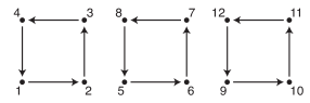
The map permutes the roots of , so the set of roots can be partitioned into -orbits. The fact that is irreducible and hence separable implies that every orbit has size four (see [24, Thm. 2.4(c)]). The roots of are thus partitioned into three orbits of size four. Labeling the roots as in Figure 1 below, we obtain an embedding whose image is the centralizer of the permutation ; see [15, pp. 2275-2277]. Denoting this centralizer by we therefore have . We will henceforth identify with .
Up to conjugacy, has exactly five maximal subgroups, which we denote by . We choose the labeling of these groups according to the following conditions, which determine the groups uniquely up to conjugation.
Here, the notation means that is isomorphic to the group labeled in the Small Groups library [2], which is distributed with the Gap [12] and Magma [3] computer algebra systems. This implies, in particular, that is the order of .
In addition to the groups , we will need to work with the maximal subgroups of these groups. The group has five maximal subgroups up to conjugation, which we denote by . In order to uniquely identify these groups it does not suffice to consider only their orders or their isomorphism types. Thus, we will refer to properties of the cycle decompositions of their elements. The labeling of the is chosen according to the following conditions:
-
•
, ;
-
•
and has an element whose disjoint cycle decomposition is a product of six 2-cycles;
-
•
and does not have an element whose disjoint cycle decomposition is a product of six 2-cycles.
The group has seven maximal subgroups up to conjugation, which we denote by . We choose the labeling as follows:
-
•
, , ;
-
•
and has an element with cycle decomposition of the form ;
-
•
and does not have an element with cycle decomposition of the form ;
-
•
and has an element with cycle decomposition of the form ;
-
•
and does not have an element with cycle decomposition of the form .
The group has five maximal subgroups up to conjugation, which we denote by . We label these subgroups according to the conditions
The group has three maximal subgroups up to conjugation, which we denote by . The labeling is chosen as follows:
Finally, the group has three maximal subgroups up to conjugation, which we denote by and label according to the properties
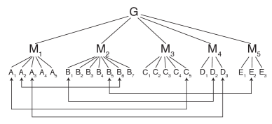
Some of the groups listed above are conjugate in . In particular, we note the following pairs of conjugate subgroups of :
| (4.1) |
We summarize some of the above information in Figure 2.
4.2. Curves corresponding to subgroups of
To every subgroup of we associate an affine algebraic curve as follows. Let be the fixed field of , let be a primitive element for the extension such that is integral over , and let be the minimal polynomial of over . Then the curve corresponding to is given by the equation . In practice, the polynomial can be computed using the methods discussed in Remark 3.5.
In this section we will determine the rational points on the curves corresponding to several of the subgroups of defined in §4.1. All of the curves we need to consider are either rational, elliptic, or hyperelliptic. An important tool in what follows is an algorithm for computing a parametrization of a given rational curve; we refer the reader to [29, Chap. 4] for a discussion of the algorithmic aspects of this problem. For our computations we have used the Parametrization function in Magma. All of the elliptic curves that arise have rank 0, so it is a straightforward calculation to determine their rational points. For the hyperelliptic curves, the methods we use to find their rational points are discussed in §5.
We begin by considering the curves corresponding to the maximal subgroups . Computing the fixed fields of these groups we obtain the following polynomials:
The curve associated to is given by the equation . We will now determine the rational points on these five curves.
Lemma 4.1.
Let denote the affine plane curve defined by . Let and be the rational functions defined in (1.2). Then the sets of rational points on the curves are given by
| (4.3) | ||||
| (4.4) | ||||
| (4.5) | ||||
| (4.6) |
Proof.
The curve is parametrizable. Indeed, the rational maps
given by and are inverses. By a simple calculation we find that the pullback of 0 under contains no rational point of ; (4.3) now follows easily.
The curve is also parametrizable. Solving for in the equation we obtain ; this implies (4.4).
Let be the elliptic curve . There is a birational map given by , where
The curve has Cremona label 20a1. This curve has rank 0, and its affine rational points are , , and . Note that any rational point on different from is mapped by to one of these five points. Pulling back all the affine rational points on we obtain (4.5).
The projective closure of is the elliptic curve with Cremona label 108a2, which has a trivial Mordell-Weil group. It follows that .
The curve is an affine model for a hyperelliptic curve whose Jacobian has rank 0. Computing the rational points on we find that . Hence , and (4.6) is proved. ∎
Next we will determine the rational points on the curves corresponding to the groups , , , , , and . The fixed fields of these subgroups of are generated by the polynomials defined in Lemmas 4.2-4.7. Hence the curves , etc. defined in these lemmas are the curves corresponding to the above subgroups.
Lemma 4.2.
Let , where
Let be the affine curve defined by the equation . Then
Proof.
Let be the curve in defined by the equations
Note that there is a map given by , and that every rational point on lifts to a rational point on .
Suppose that and let be a rational number such that . If , then , so the equation implies that . Hence .
Assuming now that , we may define
It follows from the equation and the factorization
that . Let be the affine curve defined by
The curve is parametrizable. Indeed, there are inverse rational maps and given by
It is now a straightforward calculation to verify that
| (4.7) |
Since is a rational point on , then either or there exists such that . In the former case the equation becomes , so . Thus we have found the point .
Assume now that for some . If , then and we again obtain the point . If , then expressing , and in terms of , the equation implies that
Setting we arrive at the equation
By Proposition 5.3 this implies that , which is a contradiction. Hence the points and are the only rational points on . ∎
Lemma 4.3.
Let , where
Let be the affine curve defined by the equation . Then
Proof.
Let be the curve in defined by the equations
There is a projection map given by , and every rational point on lifts to a rational point on .
Suppose that lifts to . If , then , so the equation implies that . Thus we have found the point .
Assuming now that , we may define .
From the equation and the factorization
it follows that . Thus , where is the curve defined in the proof of Lemma 4.2. By (4.7), either or for some . In the first case the equation becomes , so . This yields the point .
Suppose now that for some . Expressing , , and in terms of , the equation implies that
Letting we obtain
The above equation defines a hyperelliptic curve whose Jacobian has rank 0. Computing the rational points on the curve we obtain only the two points . It follows that , which is a contradiction. Hence the only rational points on are and . ∎
Lemma 4.4.
Let , where
Let be the affine curve defined by the equation . Then
Proof.
Let be the curve in defined by the equation
Note that there is a map , . The curve is parametrizable; a birational map is given by
Computing an inverse of we find that is defined at every rational point on different from , and that the pullback of 0 under contains no rational point on .
Suppose that . Clearly , so we may define . Since , we have ; in particular
Letting we obtain . By Proposition 5.4 this implies that , so and therefore . Hence . ∎
Lemma 4.5.
Let , where
Let be the affine curve defined by the equation . Then
Proof.
Let be the curve in defined by the equation
There is a birational map given by
Computing an inverse for we obtain the map defined by
Outside the set , is defined at every rational point on , and there is no rational point on mapped by to or .
Suppose that . Then and clearly
so we may define and then . Hence ; in particular
Letting we obtain
The hyperelliptic curve defined by this equation is isomorphic to the elliptic curve with Cremona label 20a2 and therefore has exactly six rational points. A search for points on yields
It follows that , so and therefore . Hence . ∎
Lemma 4.6.
Let , where
Let be the affine curve defined by the equation . Then
Proof.
Let be the curve in defined by the equation
The curve is parametrizable; a pair of inverse maps and is given by
We find that is defined at every rational point on , and there is no such point mapping to . Hence every rational point on has the form for some .
Suppose that . Then , so there exists , , such that ; in particular
Letting we obtain
This equation defines a hyperelliptic curve of genus 2 whose Jacobian has rank 1. A Chabauty computation222For curves of genus 2 whose Jacobian has rank 1, the set of rational points can be determined using the Chabauty function in Magma; see §5 for further details. shows that the affine rational points on the curve are and . It follows that and therefore , so . Hence . ∎
Lemma 4.7.
Let and let be the affine curve defined by the equation . Then
where is the rational function defined in (1.2).
Proof.
The equation can be solved for to obtain . ∎
Having determined the rational points on all the necessary curves, we proceed to the proof of our main result.
4.3. Classification of Galois groups
In this section we apply the techniques of §3 to study the specializations of the polynomial . We will use here much of the same notation as in §3. Thus, is the discriminant of , is a splitting field of , and . For , denotes the specialized polynomial , and , denote the Galois group and factorization type of . The ideal is denoted by . If is a prime of , then denotes the decomposition group of over . Finally, the exceptional set of is the set consisting of all rational numbers for which either is reducible or is not isomorphic to .
The rational functions defined in (1.2) will play a prominent role in what follows. Recall that denotes the set of all rational numbers of the form where , and similar notation applies to and .
Proposition 4.8.
The exceptional set of is given by
Proof.
We apply Proposition 3.4 to the polynomial . As seen in §§4.1-4.2, the group has five maximal subgroups up to conjugacy, and their fixed fields are generated by the polynomials defined before Lemma 4.1. The only rational root of is , and the discriminants of the have no rational roots. Thus, for we know that is in if and only if one of the polynomials has a rational root, or equivalently, is the first coordinate of a rational point on one of the curves . Hence, Lemma 4.1 implies that
This equivalence also holds for , since the polynomial is reducible and . To prove the proposition it remains only to observe that . ∎
Lemma 4.9.
The intersection of and is given by
Proof.
Note that , so . Suppose now that satisfy . Then we have
Letting , the above equation implies that
This equation defines a hyperelliptic curve of genus 2 whose Jacobian has rank 1. A Chabauty computation shows that the only affine rational points on the curve are and . It follows that and therefore . ∎
We can now begin to determine the structure of the groups and the factorization types for all .
Proposition 4.10.
Suppose that . Then and .
Proof.
Recall that . As seen in §4.2, the fixed field of has the form , where is a root of the polynomial . Letting we then have and .
We now apply Proposition 3.6 with and . Note that the polynomial is monic and irreducible and has as a root. In the notation of Proposition 3.6 we have .
Since , we may write for some . It is easy to see that , so . Moreover, has no rational root, so . Hence, by part (1) of Proposition 3.6 there exists a prime of dividing such that .
Letting we find that is irreducible of degree 12, and the only rational root of is 0. Hence .
We claim that . Assuming this for the moment, part (3) of Proposition 3.6 implies that and , which is what we wish to prove. Thus, it remains only to show that .
In what follows we will replace by a conjugate ideal whenever necessary. Suppose by contradiction that is a proper subgroup of . Then is contained in one of the groups . We consider each case separately.
If , then by (4.1) we have and hence . We now apply Proposition 3.3 with . Recall that the fixed field of is generated by a root of the polynomial defined in §4.2. The discriminant of has no rational root, so . By Proposition 3.3, the polynomial must have a rational root. Thus (4.5) implies that or . However, this contradicts the hypotheses since neither 0 nor are in .
If , then by (4.1) we have and hence , so has a rational root. Since also , then has a rational root. Now (4.3) and (4.4) imply that , so by Lemma 4.9. However, this again contradicts the hypotheses.
If , then by (4.1) we have and hence , so has a rational root. However, this is impossible by (4.6).
Finally, if is contained in either or , then Lemmas 4.2 and 4.3 imply that or . We have already observed that cannot be , and for one can verify directly that has order 192. By Lemma 3.2 this implies that has order 192, so cannot be contained in or . Thus we have a contradiction.
Since every case has led to a contradiction, we conclude that , as claimed. ∎
Next we determine the Galois groups and factorization types when . Note that , so that . As we will see, the analysis when differs depending on whether or not.
Proposition 4.11.
Suppose that and . Then and .
Proof.
Recall that . As seen in §4.2, the fixed field of has the form , where is a root of the polynomial . Letting we then have and .
We now apply Proposition 3.6 with and . The polynomial is monic and irreducible and has as a root. Moreover, has no rational root.
Since we may write for some . Given that , we have . Thus part (1) of Proposition 3.6 implies that there exists a prime of dividing such that .
Letting we find that factors as
| (4.8) |
where is irreducible of degree 8 and
is also irreducible. Hence . The only rational roots of are 0 and 2, so since would imply that , a contradiction.
We claim that . Assuming this for the moment, part (3) of Proposition 3.6 implies that and , which is what we wish to prove. Hence the proof will be complete if we show that .
In what follows we will replace by a conjugate ideal whenever necessary. Suppose by contradiction that is a proper subgroup of . Then is contained in one of the groups .
If , then by (4.1) we have and hence . By Proposition 3.3 applied to , this implies that the polynomial has a rational root. However, this is impossible by (4.6).
If were contained in , , or , then Lemmas 4.4-4.6 would imply that , which contradicts the hypotheses.
If , then by (4.1) we have and hence , so has a rational root. However, this is impossible by (4.6).
If , then by (4.1) we have and hence , so has a rational root. Since also , the polynomial has a rational root, so (4.3) and (4.4) imply that . Thus by Lemma 4.9. However, this contradicts the hypotheses.
Finally, if , then Lemma 4.7 implies that , a contradiction.
Since every case has led to a contradiction, we conclude that , as claimed. ∎
To complete our analysis of the groups and factorization types it remains to consider the case where . In this case the group will be isomorphic to a subgroup of , and we claim that in fact . To prove this we could proceed by contradiction as above and consider the curves corresponding to the maximal subgroups of . Unfortunately, the problem of finding all the rational points on these curves becomes unmanageable, so we will take a slightly different approach. We begin by proving two auxiliary results.
Lemma 4.12.
Let be defined by the factorization (4.8). Then for all the polynomial is irreducible and its Galois group satisfies .
Proof.
Factoring and computing its Galois group we find that is irreducible and . The group has exactly three maximal subgroups, all of index 2. The fixed fields of these subgroups are generated by the polynomials
The discriminants of the are given by
We will now use Proposition 3.4 to determine the exceptional set of . A simple calculation shows that if , then is not a root of the discriminant of nor of its leading coefficient, and that for . Hence Proposition 3.4 implies that if and only if one of the polynomials has a rational root.
If has a rational root, then is a square, so there exists such that . The hyperelliptic curve defined by this equation is isomorphic to the elliptic curve with Cremona label 108a1, which has exactly three rational points. Thus has three rational points, which must be the two points at infinity and the point . Hence , which is a contradiction.
If has a rational root, then there exists such that
The hyperelliptic curve defined by this equation is isomorphic to the elliptic curve with Cremona label 20a2, which has exactly six rational points. Thus has six rational points, which must be the two points at infinity and the points and . Since , this implies .
If has a rational root, then there exists such that
The hyperelliptic curve defined by this equation is isomorphic to the curve from Proposition 5.4. Since has exactly five rational points, the same holds for . A search for points on then shows that its only affine rational points are and . Hence .
We conclude from the above discussion that if , then , and therefore is irreducible and . ∎
Proposition 4.13.
Suppose that . Then and .
Proof.
Recall that
The fixed field of has the form , where is a root of the polynomial . Thus and .
We now apply Proposition 3.6 with and . Note that
is monic and irreducible and has as a root. Moreover, the discriminant of has no rational root. Since , we may write for some . By part (1) of Proposition 3.6 there exists a prime of dividing such that .
Let , so that , and let
From the factorization (4.8) it follows that , where
One can verify that and that is irreducible of degree 8. Factoring we find that , where
and , are irreducible. Note that since . Computing the discriminant of we see that its only rational roots are . Hence .
We claim that . Assuming this for the moment, part (3) of Proposition 3.6 implies that and , which is what we have to prove. Thus it remains only to show that .
Since is a subgroup of and , it suffices to show that . We know by Lemma 3.2 that is isomorphic to , so we may show instead that the splitting field of has degree 64 over . Let denote this splitting field.
Let , so that . From our work above we deduce that, up to a nonzero scalar,
Hence is the compositum of the splitting fields of and . Note that and split over the same field, namely
This field is equal to if and only if there exists such that
The hyperelliptic curve defined by this equation has a Jacobian of rank 0; computing the points on the curve we find that its only affine rational points are and . Since , we conclude that is a quadratic field.
Let be the splitting field of . By Lemma 4.12 we know that . Since , we will have unless . We will now rule out this possibility and thus complete the proof.
As seen in the proof of Lemma 4.12, the group has exactly three subgroups of index 2; by the lemma the same is true for . Hence the field has exactly three subfields of degree 2 over . Now, the quadratic extensions of that lie inside the splitting field of are generated by the polynomials listed in the proof of Lemma 4.12. Specializing at we conclude that the polynomials all have a root in . Hence contains the fields , where
From our work in the proof of Lemma 4.12 we deduce that the are quadratic fields, and all distinct. Hence these must be the three quadratic fields contained in . We claim that none of these fields can be equal to .
Using the relation we see that , where
and . Suppose that for some . Then is a rational square. It follows that there exists such that one of the following holds:
Summarizing our work up to this point we obtain a proof of Theorem 1.2.
Theorem 4.14.
Let . Then the following hold:
-
(1)
If and , then and .
-
(2)
If , then and .
-
(3)
Suppose that . Then the following hold:
-
(a)
If , then and .
-
(b)
If , then and .
-
(a)
Proof.
For the numbers that are excluded in Theorem 4.14, the Galois group can be computed using an algorithm of Fieker and Klüners [11] that is implemented in Magma. Carrying out these Galois group computations and factoring to find the factorization types , we obtain the data summarized in Table 1 below. For each number we give a pair such that is isomorphic to the group labeled in the Small Groups library [2]; thus represents the order of .
| -5 | -5/2 | -155/72 | -2 | -5/4 | 0 | 19/16 | |
|---|---|---|---|---|---|---|---|
4.4. Density results
For every polynomial , let denote the set of all prime numbers such that has a root in . The Chebotarev Density Theorem implies that the Dirichlet density of , which we denote by , exists and can be computed if the Galois group of is known. More precisely, we have the following lemma.
Lemma 4.15.
Let be a separable polynomial of degree . Let be a splitting field for , and set . Let be the roots of in and, for each index , let denote the stabilizer of under the action of . Then the Dirichlet density of is given by
| (4.9) |
Proof.
This follows from Theorem 2.1 in [15]. ∎
We deduce from Lemma 4.15 that the value of can be determined if a permutation representation of (induced by a labeling of the roots of ) is known. Indeed, if is a subgroup of the symmetric group such that , then can be computed using (4.9) by replacing with and with , the stabilizer of in . This fact reduces the problem of computing to the problem of computing a permutation representation of . The latter can be done using the algorithm of Fieker and Klüners referenced above. Hence it is in principle possible to evaluate for any polynomial .
Returning now to dynatomic polynomials, Theorem 4.14 provides a permutation representation of the Galois group of for all but seven rational numbers . Thus, we may use this theorem together with Lemma 4.15 to compute the density of the set for almost all . To simplify notation we will henceforth write instead of .
Theorem 4.16.
Let .
-
(1)
If and , then .
-
(2)
If , then .
-
(3)
Suppose that . Then the following hold:
-
(a)
If , then .
-
(b)
If , then .
-
(a)
Proof.
For the numbers that are excluded in Theorem 4.16, the density of can be found by first computing the Galois group of and then applying Lemma 4.15. Carrying out these computations we obtain the density values shown in Table 2.
| -5 | -5/2 | -155/72 | -2 | -5/4 | 0 | 19/16 | |
|---|---|---|---|---|---|---|---|
| 23/64 | 1/6 | 1/2 | 11/32 | 39/64 | 1/4 | 27/64 |
We end this section with an application of the density results obtained above. By a well-known theorem of Morton [23], a quadratic polynomial over cannot have a rational point of period four. We can now prove Theorem 1.3, thus showing that there is a strong local obstruction explaining Morton’s result.
Corollary 4.17.
Let be a quadratic polynomial. Then, for more than of all primes , does not have a point of period four in .
Proof.
Let be the unique rational number such that is linearly conjugate to . The polynomials and factor in the same way over every extension of (see [15, Cor. 2.11]); in particular has a root in a -adic field if and only if has a root in . From Theorem 4.16 and Table 2 we deduce that
Thus, more than of all primes are in the complement of . Now, if , then does not have a root in , so does not have a root in , and therefore does not have a point of period four in . ∎
5. Rational points on hyperelliptic curves
In this section we describe the methods used to determine the rational points on the various hyperelliptic curves that arise in the proof of Theorem 4.14. In addition we provide detailed arguments for five of these curves.
5.1. Preliminaries
Let be a hyperelliptic curve over of genus . By Faltings’s Theorem the set is finite. The question we are concerned with here is how to provably determine all the rational points on . The techniques used for this differ depending on whether is empty or not.
Suppose first that and we need to prove this. An initial step is to test whether has a point over every completion of . This can be done algorithmically, and the necessary algorithms have been implemented; see [5, §5], for instance. The Magma functions HasPoint and HasPointsEverywhereLocally can be used to determine whether has points over a given -adic field or over all -adic fields. These methods are used in the proofs of Propositions 5.3, 5.6, and 5.7 below.
If we find that fails to have a point over for some , then . However, it may occur that has a point in every -adic field and yet has no rational point. In that case we can apply the two-cover descent [6] or Mordell-Weil sieve [7] techniques to try to show that is empty. An implementation of the former method is available via the Magma function TwoCoverDescent. The algorithm determines a collection of covers of such that any rational point on lifts to one of the covers. In particular, if the algorithm has empty output, then must be empty. We have applied this method in the proofs of Propositions 5.3 and 5.7.
Suppose now that does have a rational point, and we need to determine all rational points. It is useful for this purpose to know the structure of the Mordell-Weil group , where is the Jacobian variety of . In particular, the rank of this group should be determined if possible. An upper bound for can be obtained by using a descent argument as in [32], and a lower bound by searching for independent rational points on . If , then it is a finite calculation to determine all rational points on . If the problem becomes much harder, though still possible to handle in certain cases. Most importantly for our purposes, if , then one may be able to apply Chabauty techniques (described below) to obtain an upper bound for the number of rational points on . If this upper bound matches the number of known points, then has been determined. If the upper bound obtained is larger than the known number of rational points, then a Mordell-Weil sieve argument might improve the bound.
Magma includes several functions that can be used to carry out the above calculations. The RankBound function computes an upper bound for , and if is known to be 0, then the Chabauty0 function determines all rational points on . These tools are used in the proofs of Lemmas 4.1 and 4.3, and Propositions 4.13 and 5.6. If and , then the Chabauty function uses a combination of the Chabauty-Coleman method with a Mordell-Weil sieve to compute the set . This method is used in the proofs of Lemmas 4.6 and 4.9, and Proposition 5.7.
5.2. The method of Chabauty and Coleman
Let be a smooth, projective, geometrically integral curve over of genus , and suppose that has a rational point. The goal of the method is to find an upper bound for . We begin by considering the reduction of modulo a prime.
Let be a prime of good reduction for , and let be the minimal proper regular model333See [19, §10.1.1] or [31, Chap. IV, §4] for background on models of curves. of over . We denote the set of -points on the special fiber of by . The model gives rise to a surjective reduction map444See [19, §10.1.3] for the definition and properties of the reduction map. which we denote by . The preimage of a point under this map will be called a residue disk. Clearly the residue disks form a finite partition of , so in order to bound it suffices to bound the number of rational points within each residue disk. To accomplish the latter we use integration of global differentials on .
Let be the Jacobian variety of . Recall that the -vector space of global 1-forms on has dimension , and that there is a canonical isomorphism
| (5.1) |
To every global 1-form on there corresponds a unique analytic homomorphism such that ; see [33, Lemma 3.2]. Using this map we define, for points ,
The integral thus defined satisfies the usual properties one might expect. In particular, it is linear in the integrand and changes sign if the limits of integration are interchanged. See Proposition 2.4 in [9] for these and other properties.
A central object in the method of Chabauty and Coleman is the annihilator of , which is defined to be the -vector space
An important step in the method is to find a nontrivial 1-form in this space. The existence of such a form is guaranteed if , where is the rank of the group . Indeed, this can be deduced from the following lemma, which we include for later reference. The proof is a simple exercise in linear algebra.
Lemma 5.1.
Let form a basis for . Suppose that generate a subgroup of finite index in . Let be the matrix with entries . Then the linear isomorphism given by restricts to an isomorphism .
Now let be a global 1-form on , and let be the 1-form on corresponding to under the isomorphism (5.1). For any points we set
It follows from the definitions that if , then
| (5.2) |
This property of annihilating differentials will allow us to obtain an upper bound for . Recall that the general strategy is to find an upper bound for the number of rational points in every residue disk. We can now describe precisely how to do this.
Suppose that , so that is nontrivial, and let be a residue disk. In order to find an upper bound for the cardinality of the set we begin by choosing a basepoint and a global differential on corresponding to a 1-form in . We impose no restriction on , but for reasons mentioned below we require that
| (5.3) | reduces to a nonzero global differential on . |
Let be the function defined by the formula
By (5.2) this function vanishes on . It therefore suffices to find a bound for the number of zeros of . To do this we choose a point and a local parameter at , i.e., a generator of the maximal ideal of the local ring . We require that
| (5.4) | reduces to a local parameter at the point . |
This assumption ensures that is regular on and induces a bijection . We may thus regard as a function . The next step in the method is to find a power series representation for this function.
By embedding the local ring in its completion we can represent every rational function in as a formal power series in , and every rational function in as a formal Laurent series in with -coefficients555More precisely, there is a -algebra isomorphism mapping to . This induces an isomorphism of with the field of fractions of , into which naturally embeds. See [8, p. 128] for proofs of these statements..
We may write for a unique rational function . The condition (5.3) implies that the power series representation of has -coefficients, and that these are not all zero modulo . Thus
with for all , and for some . Formal antidifferentiation now yields a power series representation for :
| (5.5) |
where the constant term is necessarily given by . Recall that our goal is to bound the number of zeros of in . It is helpful for this purpose to define an auxiliary function by . From (5.5) we obtain the power series representation
We can apply Straßmann’s Theorem [13, Thm. 4.4.6] to find an upper bound for the number of zeros of (and hence the number of zeros of ). Defining an index uniquely by the conditions
the theorem guarantees that has at most zeros in , and therefore
This accomplishes our goal of finding a bound for the number of rational points in . By applying this process to every residue disk we then obtain an upper bound for .
Remark 5.2.
In order to determine the value of one only needs to know finitely many of the coefficients . Indeed, it is a simple exercise to show that if is large enough, then
| (5.6) |
With as above, let be the quantity on the right-hand side of (5.6). Note that for all we have
It follows from the choice of that for all . This implies that . Moreover, since , we must have . Thus can be determined if the coefficients are known.
5.3. Explicit Chabauty for hyperelliptic curves
Though the technique described above can in theory be applied to a fairly general curve , in practice there are several issues that make it difficult to carry out the necessary computations. For hyperelliptic curves, however, there are tools available which in many cases make it possible to explicitly compute all of the required data.
We assume henceforth that is a hyperelliptic curve given by an equation , where has odd degree and the genus is at least 2. Let be a prime not dividing the discriminant of , so that has good reduction at . Work of Balakrishnan-Bradshaw-Kedlaya [1] provides an algorithm for computing the integral for any points and any global differential on ; an implementation of the algorithm is included in Sage [10]. By using this tool it is possible to automate a significant portion of the calculations required for a Chabauty-Coleman argument.
To begin we assume that the rank of has been determined, and that . From our discussion in the previous section we deduce the following steps for bounding the number of rational points on .
-
(1)
Determine a basis for the annihilator of .
-
(2)
Choose a basepoint .
- (3)
By adding all the bounds computed in step 3f we obtain an upper bound for . We will now discuss how to explicitly carry out each of the above steps.
Step 1. Since this will always be the case in the examples worked out in this paper, let us assume that we know pairs of points such that the divisor classes generate a subgroup of finite index in .
A basis for the global differentials on is given by
Let be the matrix with entries
Computing the entries of and a basis for , Lemma 5.1 can be applied to obtain a basis for . If necessary, we then scale the basis differentials to ensure that they reduce to nonzero global differentials on . Let be a basis for constructed in this way. Note that any one of the ’s can be chosen as the differential in step 3c. More generally, can be any linear combination of the ’s satisfying (5.3).
Step 3a. If is the point at infinity, then we lift to . Otherwise we apply Hensel’s Lemma. Let have coordinates . If we lift to a square root of in . If we lift to a root of in .
Step 3b. Assuming the lift of was constructed as above, we choose the local parameter at as follows:
Step 3d. Recall that was constructed as a linear combination of the differentials from Step 1, say . Expressing each as a linear combination of we can write for some polynomial . Thus, letting we have
| (5.7) |
In order to express in the form it suffices to find the Laurent series for and in powers of . Indeed, writing and we can find the Laurent series, say , for the rational function . Then (5.7) yields , where is the formal derivative of .
It remains to explain how the Laurent series for and are computed. Suppose first that is an affine point with . The local parameter at is , so the power series for is . Now, Hensel’s Lemma implies that there is a unique power series such that and ; this is the series for .
Similarly, if is of the form , then the local parameter is , which gives the power series for . The series for is the unique power series such that and .
Finally, if is the point at infinity, then the local parameter is . Let be the polynomial , so that the complementary affine patch of is given by . Let and be the power series for and at the point . The Laurent series for and are then and .
Step 3f. In view of Remark 5.2, once enough of the terms of the power series have been determined, it is a straightforward calculation to find the Straßmann bound.
We proceed now to apply all of the methods discussed above to determine the rational points on five curves.
5.4. Rational points on five curves
Proposition 5.3.
Let be the hyperelliptic curve over defined by the equation , where
The set of affine rational points on is .
Proof.
The polynomials and have no rational root. Hence, if is an affine rational point on , then and are nonzero, and since their product is a square, they must have the same squarefree part, say . Thus, we have and for some .
For every squarefree integer , let be the curve
Note that there is a map . The above argument shows that every affine rational point on lifts to for some .
We can narrow down the possibilities for . Suppose that lifts to a point . If is a prime dividing , it is easy to see that . Reducing the equations and modulo , we conclude that and have a common root modulo , and therefore divides the resultant of and . The prime divisors of are 2, 5, and 17, so can only be divisible by these primes. It follows that
Thus, in order to determine it suffices to determine for every . Let and be the hyperelliptic curves
and for every let denote the quadratic twists of by . Note that there are projection maps
In particular this implies that if or , and in any case the rational points on can be determined if is known. We will now determine for every .
Consider first . A search for points of small height on yields the points . A 2-descent shows that the rank of is at most 1. The divisor class has infinite order, so in fact the rank of is 1. A Chabauty argument combined with a Mordell-Weil sieve now shows that . Lifting these points to we conclude that
By a similar argument we obtain .
We claim that for every . To prove this we will mostly use local arguments to show that either or .
For we have , and for , . For we find that . Finally, for , a 2-cover descent calculation for the curve returns an empty fake 2-Selmer set (in the terminology of [6]); hence .
To summarize, we have shown that for every except . Thus, every affine rational point on lifts to a rational point on either or . Mapping the points and to we conclude that . ∎
Proposition 5.4.
Let be the hyperelliptic curve over defined by
The set of affine rational points on is .
Proof.
A search for points on yields the five points . We aim to show that , so that these are all the rational points on . To prove this bound we will use a Chabauty-Coleman argument with the prime , which is a prime of good reduction for . We apply the method as described in §5.3.
Let be the Jacobian variety of . Our first step is to find generators for a subgroup of finite index in . By a 2-descent calculation we find that the rank of is at most 1. The divisor class can be shown to have infinite order, so the rank is equal to 1, and generates a subgroup of finite index in .
Next we find a suitable basis for the annihilator of . Using the basis
for the global differentials on and computing the entries of the matrix
we obtain
The vectors and form a basis for the kernel of , so Lemma 5.1 implies that the differentials and form a basis for . Scaling these differentials so that they will be nonzero modulo 11, we obtain a new basis for :
Next we use the differentials and to find upper bounds for the number of rational points within each residue disk in .
The points on the reduction of modulo 11 are the following:
For each residue disk above one of these points we will choose a differential and compute an upper bound for the number of zeros of the function in . Our goal is to choose in such a way that either , in which case , or when we know that contains a rational point. By trial and error, choosing various linear combinations of and , we have found such a differential for every residue disk. We summarize the results of our calculations in Table 3 below. The table contains, for every differential and every point , the computed upper bound for the number of zeros of the function in the residue disk above .
| 5 | 1 | 1 | 1 | 1 | 1 | 1 | |
| 1 | 2 | 1 | 1 | 1 | 1 | 0 | |
| 1 | 1 | 1 | 1 | 0 | 1 | 1 | |
| 1 | 1 | 0 | 1 | 1 | 1 | 1 |
For the residue disks containing a known rational point – namely those above , and – we can conclude from the above data that . Indeed, either or provides an upper bound of 1 for the number of rational points in .
For the residue disks above , , and we can conclude that , since at least one of the chosen differentials provides an upper bound of 0.
At this stage we know that , since the data does not rule out rational points above . However, must be odd since has no affine rational Weierstrass point. Therefore , which completes the proof.
As an example, we include the details of one of the computations needed to fill in Table 3. For the reader interested in reproducing our results, the Sage code used for all of the calculations is available in [16].
Let us show that integration of rules out rational points in the residue disk above the point . Lifting to a point in we obtain the point
A local parameter at is . Expanding and in powers of we have and , where
Expressing in the form and using the above expansions for and , we find that , where
Next, we construct the power series , where is the formal antiderivative of . We obtain , where
The bound (5.6) is satisfied with , so these coefficients are enough to determine the Straßmann bound for . Clearly has the minimal valuation among the coefficients of , and there is no other coefficient with equal valuation. Hence the Straßmann bound is 0, as claimed. ∎
Proposition 5.5.
Let be the hyperelliptic curve over defined by
The set of affine rational points on is
Proof.
We claim that the number of rational points on must be a multiple of 4. Let denote the hyperelliptic involution on . Note that has an automorphism given by . Since , has order 4. Neither , , nor have rational fixed points, so the orbit of every point in under must consist of exactly four points. This implies our claim.
We will now use the method of Chabauty and Coleman to show that and therefore, in view of the above, . Since we already know 12 rational points on (namely the two points at infinity and the ten affine points listed above), this will prove that , from which the proposition follows.
For the Chabauty argument we use the prime . Given that is not defined by a model of odd degree, we begin by making a change of variables in order to be able to apply the Coleman integration algorithms from [1]. Let denote a square root of in the field . The change of variables
induces an isomorphism (defined over ), where is a hyperelliptic curve over defined by an equation of the form
The map gives rise to a pullback isomorphism
To simplify notation we will henceforth write instead of .
Using the model and the integration algorithms from [1] we can compute Coleman integrals on . Indeed, by the change of variables formula (see [9, Thm. 2.7]) we have
for all points and every global differential on . With this observation in mind, we proceed to find an upper bound for .
Let be the Jacobian variety of . A 2-descent computation shows that the rank of is at most 2. Since the genus of is 4, this guarantees that is nontrivial. We will now find a basis for the annihilator.
Note that the two rational points at infinity on are mapped by to the points on . Let and .
Let be the differentials on given by . Computing the entries of the matrix
we find that the 13-adic valuations of the entries of are in the first row and in the second row. It follows that the rows of are linearly independent, and therefore has rank 2.
The fact that the entries of are nonzero implies that the divisor classes and have infinite order in . Moreover, since has rank 2, and must be linearly independent over . (Any relation of the form for nonzero integers and would imply that the rows of are linearly dependent.) We can therefore conclude that and generate a subgroup of finite index in .
Since has rank 2, the kernel of has dimension 2. Computing a basis for the kernel we obtain the vectors and , where
By Lemma 5.1, the differentials
form a basis for the annihilator of . Thus we have
| (5.8) |
Let denote the set . We aim to show that . For every global differential on we define a function by the formula . By (5.8), if is a linear combination of and , then vanishes on .
For every residue disk we will choose a differential on , constructed as a linear combination of and , and determine an upper bound for the number of zeros that the function has in . Since is hyperelliptic and is given by a model of odd degree, a bound can be computed as discussed in §5.3. Let denote the bound thus obtained.
We summarize the results of our calculations below. The code used for all of these computations is available in [16].
Mapping the 12 known rational points on into using the map and then reducing modulo 13, we obtain the set
The set of -points on the reduction of is given by
For every residue disk above a point in we compute . Hence each one of these 12 residue disks contains exactly one point in .
For the residue disks above and above we also obtain . Hence each one of these disks contains at most one point in .
Finally, for the residue disks above we find that , and for those above we obtain . Hence these residue disks do not intersect .
We conclude that and therefore , as desired. ∎
Proposition 5.6.
Let be the hyperelliptic curve over defined by the equation , where
The set of affine rational points on is .
Proof.
For every squarefree integer , let be the curve
Note that there is a map given by . Suppose that is an affine rational point on with . Then and are nonzero and . Thus and have the same squarefree part, say , so there exist such that .
The prime divisors of are , and 17, so can only be divisible by these primes. Furthermore, only takes positive values for , so must be positive. Therefore
Let and be the hyperelliptic curves and , respectively. We denote by the quadratic twist of by . Since , the curve has a rational point. Now, for we find that if , and if . Hence we must have .
Since , then , so is the first coordinate of a rational point on . Now, the Jacobian of has rank 0; this allows us to show that the affine rational points on are and . Since we are assuming , this implies that . Solving we obtain and therefore . ∎
Proposition 5.7.
Let be the hyperelliptic curve over defined by the equation , where
The set of affine rational points on is .
Proof.
Suppose that is a rational point on with , and let be the common squarefree part of and . The prime divisors of are 2, 5, and 17. Moreover, only takes positive values for , so must be positive. Therefore
Let and , respectively, denote the hyperelliptic curves defined by and .
For , and we find that , and for we have . For the curve has an empty fake 2-Selmer set, so . Thus or 2.
Suppose that , so that there exists such that . Let be the hyperelliptic curve defined by
There is a map given by
Since , is defined at the point , and . Now, the Jacobian of has rank 1, and a Chabauty computation shows that has only one affine rational point, namely . Pulling this point back to we obtain no rational point on , which is a contradiction.
The only remaining possibility is that . In this case there exists such that . The same map defined above maps to the quadratic twist . The Jacobian of has rank 1, and a Chabauty computation shows that the only rational points on are and . Pulling these points back to we obtain the points . We must therefore have , and the proposition follows. ∎
Acknowledgements
The author would like to thank Joseph Wetherell for sharing Sage code used in Chabauty-Coleman calculations, and Imme Arce for her help in preparing the figures.
Appendix A Galois group data
We define here the groups appearing in our main result, Theorem 4.14. Every group is presented as a subgroup of the symmetric group by specifying generators for the group. Further information about these groups can be accessed by searching the Small Groups library [2], which is distributed with the Gap and Magma computer algebra systems. Every group in this library is identified by a pair where is the order of the group; for each group listed below we provide the corresponding identification pair.
Group
ID: . Generators:
Group
ID: . Generators:
Group
ID: . Generators:
Group
ID: . Generators:
References
- [1] Jennifer S. Balakrishnan, Robert W. Bradshaw, and Kiran S. Kedlaya, Explicit Coleman integration for hyperelliptic curves, Algorithmic number theory, Lecture Notes in Comput. Sci., vol. 6197, Springer, Berlin, 2010, pp. 16–31.
- [2] Hans Ulrich Besche, Bettina Eick, and E. A. O’Brien, A millennium project: constructing small groups, Internat. J. Algebra Comput. 12 (2002), no. 5, 623–644.
- [3] Wieb Bosma, John Cannon, and Catherine Playoust, The Magma algebra system. I. The user language, J. Symbolic Comput. 24 (1997), no. 3-4, 235–265, Computational algebra and number theory (London, 1993).
- [4] Thierry Bousch, Sur quelques problèmes de dynamique holomorphe, Ph.D. thesis, Université de Paris-Sud, Centre d’Orsay, 1992.
- [5] Nils Bruin, Some ternary Diophantine equations of signature , Discovering mathematics with Magma, Algorithms Comput. Math., vol. 19, Springer, Berlin, 2006, pp. 63–91.
- [6] Nils Bruin and Michael Stoll, Two-cover descent on hyperelliptic curves, Math. Comp. 78 (2009), no. 268, 2347–2370.
- [7] by same author, The Mordell-Weil sieve: proving non-existence of rational points on curves, LMS J. Comput. Math. 13 (2010), 272–306.
- [8] Daniel Bump, Algebraic geometry, World Scientific Publishing Co., Inc., River Edge, NJ, 1998.
- [9] Robert F. Coleman, Torsion points on curves and -adic abelian integrals, Ann. of Math. (2) 121 (1985), no. 1, 111–168.
- [10] The Sage Developers, SageMath, the Sage Mathematics Software System (Version 7.6), 2017, http://www.sagemath.org.
- [11] Claus Fieker and Jürgen Klüners, Computation of Galois groups of rational polynomials, LMS J. Comput. Math. 17 (2014), no. 1, 141–158.
- [12] The GAP Group, GAP – Groups, Algorithms, and Programming, Version 4.8.7, 2017.
- [13] Fernando Q. Gouvêa, -adic numbers, second ed., Springer-Verlag, Berlin, 1997.
- [14] Jürgen Klüners and Gunter Malle, Explicit Galois realization of transitive groups of degree up to 15, J. Symbolic Comput. 30 (2000), no. 6, 675–716, Algorithmic methods in Galois theory.
- [15] David Krumm, A local-global principle in the dynamics of quadratic polynomials, Int. J. Number Theory 12 (2016), no. 8, 2265–2297.
- [16] by same author, Code for the Chabauty computations in the article “Galois groups in a family of dynatomic polynomials”, https://github.com/davidkrumm/galois_dynatomic, 2017.
- [17] David Krumm and Nicole Sutherland, Galois groups over rational function fields and explicit Hilbert irreducibility, Preprint. Available at https://arxiv.org/pdf/1708.04932.pdf.
- [18] Serge Lang, Algebra, third ed., Graduate Texts in Mathematics, vol. 211, Springer-Verlag, New York, 2002.
- [19] Qing Liu, Algebraic geometry and arithmetic curves, Oxford Graduate Texts in Mathematics, vol. 6, Oxford University Press, Oxford, 2002.
- [20] Dino Lorenzini, An invitation to arithmetic geometry, Graduate Studies in Mathematics, vol. 9, American Mathematical Society, Providence, RI, 1996.
- [21] William McCallum and Bjorn Poonen, The method of Chabauty and Coleman, Explicit methods in number theory, Panor. Synthèses, vol. 36, Soc. Math. France, Paris, 2012, pp. 99–117.
- [22] Patrick Morton, Arithmetic properties of periodic points of quadratic maps, Acta Arith. 62 (1992), no. 4, 343–372.
- [23] by same author, Arithmetic properties of periodic points of quadratic maps, II, Acta Arith. 87 (1998), no. 2, 89–102.
- [24] Patrick Morton and Pratiksha Patel, The Galois theory of periodic points of polynomial maps, Proc. London Math. Soc. (3) 68 (1994), no. 2, 225–263.
- [25] Patrick Morton and Joseph H. Silverman, Rational periodic points of rational functions, Int. Math. Res. Not. 1994 (1994), no. 2, 97–110.
- [26] Jürgen Neukirch, Algebraic number theory, Grundlehren der Mathematischen Wissenschaften [Fundamental Principles of Mathematical Sciences], vol. 322, Springer-Verlag, Berlin, 1999.
- [27] Chatchawan Panraksa, Arithmetic dynamics of quadratic polynomials and dynamical units, Ph.D. thesis, University of Maryland, College Park, 2011.
- [28] Bjorn Poonen, The classification of rational preperiodic points of quadratic polynomials over : a refined conjecture, Math. Z. 228 (1998), no. 1, 11–29.
- [29] J. Rafael Sendra, Franz Winkler, and Sonia Pérez-Díaz, Rational algebraic curves, Algorithms and Computation in Mathematics, vol. 22, Springer, Berlin, 2008.
- [30] Jean-Pierre Serre, Topics in Galois theory, Research Notes in Mathematics, vol. 1, Jones and Bartlett Publishers, Boston, MA, 1992.
- [31] Joseph H. Silverman, Advanced topics in the arithmetic of elliptic curves, Graduate Texts in Mathematics, vol. 151, Springer-Verlag, New York, 1994.
- [32] Michael Stoll, Implementing 2-descent for Jacobians of hyperelliptic curves, Acta Arith. 98 (2001), no. 3, 245–277.
- [33] Joseph Loebach Wetherell, Bounding the number of rational points on certain curves of high rank, Ph.D. thesis, University of California, Berkeley, 1997.