Estimation of Mean Residual Life

Abstract

Yang [1978b] considered an empirical estimate of the mean residual life function on a fixed finite interval. She proved it to be strongly uniformly consistent and (when appropriately standardized) weakly convergent to a Gaussian process. These results are extended to the whole half line, and the variance of the the limiting process is studied. Also, nonparametric simultaneous confidence bands for the mean residual life function are obtained by transforming the limiting process to Brownian motion.

label=u1,url]http://www.stat.washington.edu/jaw/

t1Supported in part by NSF Grant DMS-1104832 and the Alexander von Humboldt Foundation

1 Introduction and summary

This is an updated version of a Technical Report, Hall and Wellner [1979], that, although never published, has been referenced repeatedly in the literature: e.g., Csörgő and Zitikis [1996], Berger et al. [1988], Csörgő et al. [1986], Hu et al. [2002], Kochar et al. [2000], Qin and Zhao [2007].

Let $X_{1},\ldots,X_{n}$ be a random sample from a continuous d.f. $F$ on ${\mathbb{R}}^{+}=[0,\infty)$ with finite mean $\mu=E(X)$, variance $\sigma^{2}\leq\infty$, and density $f(x)>0$. Let $\overline{F}=1-F$ denote the survival function, let ${\mathbb{F}}_{n}$ and $\overline{{\mathbb{F}}}_{n}$ denote the empirical distribution function and empirical survival function respectively, and let

$$e(x)\equiv e_{F}(x)\equiv E(X-x|X>x)=\int_{x}^{\infty}\overline{F}dI/\overline{F}(x),\ \ \ \ 0\leq x<\infty$$

denote the mean residual life function or life expectancy function at age $x$. We use a subscript $F$ or $\overline{F}$ on $e$ interchangeably, and $I$ denotes the identity function and Lebesgue measure on ${\mathbb{R}}^{+}$.

A natural nonparametric or life table estimate of $e$ is the random function $\hat{e}_{n}$ defined by

$$\hat{e}_{n}(x)=\left\{\int_{x}^{\infty}\overline{{\mathbb{F}}}_{n}dI/\overline{{\mathbb{F}}}_{n}(x)\right\}1_{[0,X_{nn})}(x)$$

where $X_{nn}\equiv\max_{1\leq i\leq n}X_{i}$; that is, the average, less $x$, of the observations exceeding $x$. Yang [1978b] studied $\hat{e}_{n}$ on a fixed finite interval $0\leq x\leq T<\infty$. She proved that $\hat{e}_{n}$ is a strongly uniformly consistent estimator of $e$ on $[0,T]$, and that, when properly centered and normalized, it converges weakly to a certain limiting Gaussian process on $[0,T]$.

We first extend Yang’s (1978) results to all of ${\mathbb{R}}^{+}$ by introducing suitable metrics. Her consistency result is extended in Theorem 2.1 by using the techniques of Wellner [1977, 1978]; then her weak convergence result is extended in Theorem 2.2 using Shorack [1972] and Wellner [1978].

It is intuitively clear that the variance of $\hat{e}_{n}(x)$ is approximately $\sigma^{2}(x)/n(x)$ where

$$\sigma^{2}(x)=Var[X-x|X>x]$$

is the residual variance and $n(x)$ is the number of observations exceeding $x$; the formula would be justified if these $n(x)$ observations were a random sample of fixed sized $n(x)$ from the conditional distribution $P(\cdot|X>x)$. Noting that $\overline{{\mathbb{F}}}_{n}(x)=n(x)/n\rightarrow\overline{F}(x)$ a.s., we would then have

$$nVar[\hat{e}_{n}(x)]=n\sigma^{2}(x)/n(x)\rightarrow\sigma^{2}(x)/\overline{F}(x).$$

Proposition 2.1 and Theorem 2.2 validate this (see (2.4) below): the variance of the limiting distribution of $n^{1/2}(\hat{e}_{n}(x)-e(x))$ is precisely $\sigma^{2}(x)/\overline{F}(x)$.

In Section 3 simpler sufficient conditions for Theorems 2.1 and 2.2 are given and the growth rate of the variance of the limiting process for large $x$ is considered; these results are related to those of Balkema and de Haan [1974]. Exponential, Weibull, and Pareto examples are considered in Section 4.

In Section 5, by transforming (and reversing) the time scale and rescaling the state space, we convert the limit process to standard Brownian motion on the unit interval (Theorem 5.1); this enables construction of nonparametric simultaneous confidence bands for the function $e_{F}$ (Corollary 5.2). Application to survival data of guinea pigs subject to infection with tubercle bacilli as given by Bjerkedal [1960] appears in Section 6.

We conclude this section with a brief review of other previous work. Estimation of the function $e$, and especially the discretized life-table version, has been considered by Chiang; see pages 630-633 of Chiang [1960] and page 214 of Chiang [1968]. (Also see Chiang [1968], page 189, for some early history of the subject.) The basis for marginal inference (i.e. at a specific age $x$) is that the estimate $\hat{e}_{n}(x)$ is approximately normal with estimated standard error $S_{k}/\sqrt{k}$, where $k=n\overline{{\mathbb{F}}}_{n}(x)$ is the observed number of observations beyond $x$ and $S_{k}$ is the sample standard deviation of those observations. A partial justification of this is in Chiang [1960], page 630, (and is made precise in Proposition 5.2 below). Chiang [1968], page 214, gives the analogous marginal result for grouped data in more detail, but again without proofs; note the solumn $S_{\hat{e}_{i}}$ in his Table 8, page 213, which is based on a modification and correction of a variance formula due to Wilson [1938]. We know of no earlier work on simultaneous inference (confidence bands) for mean residual life.

A plot of (a continuous version of) the estimated mean residual life function of 43 patients suffering from chronic gramulocytic leukemia is given by Bryson and Siddiqui [1969]. Gross and Clark [1975] briefly mention the estimation of $e$ in a life - table setting, but do not discuss the variability of the estimates (or estimates thereof). Tests for exponentiality against decreasing mean residual life alternatives have been considered by Hollander and Proschan [1975].

2 Convergence on ${\mathbb{R}}^{+}$; covariance function of the limiting process

Let $\{a_{n}\}_{n\geq 1}$ be a sequence of nonnegative numbers with $a_{n}\rightarrow 0$ as $n\rightarrow\infty$. For any such sequence and a d.f. $F$ as above, set $b_{n}=F^{-1}(1-a_{n})\rightarrow\infty$ as $n\rightarrow\infty$. Then, for any function $f$ on ${\mathbb{R}}^{+}$, define $f^{*}$ equal to $f$ for $x\leq b_{n}$ and $0$ for $x>b_{n}$: $f^{*}(x)=f(x)1_{[0,b_{n}]}(x)$. Let $\|f\|_{a}^{b}\equiv\sup_{a\leq x\leq b}|f(x)|$ and write $\|f\|$ if $a=0$ and $b=\infty$.

Let ${\cal H}(\downarrow)$ denote the set of all nonnegative, decreasing functions $h$ on $[0,1]$ for which $\int_{0}^{1}(1/h)dI<\infty$.

Condition 1a. There exists $h\in{\cal H}(\downarrow)$ such that

$$M_{1}\equiv M_{1}(h,F)\equiv\sup_{x}\frac{\int_{x}^{\infty}h(F)dI/h(F(x))}{e(x)}<\infty.$$

Since $0<h(0)<\infty$ and $e(0)=E(X)<\infty$, Condition 1a implies that $\int_{0}^{\infty}h(F)dI<\infty$. Also note that $h(F)/h(0)$ is a survival function on ${\mathbb{R}}^{+}$ and that the numerator in Condition 1a is simply $e_{h(F)/h(0)}$; hence Condition 1a may be rephrased as: there exists $h\in{\cal H}(\downarrow)$ such that $M_{1}\equiv\|e_{h(F)/h(0)}/e_{F}\|<\infty$.

Condition 1b. There exists $h\in{\cal H}(\downarrow)$ for which $\int_{0}^{\infty}h(F)dI<\infty$ and $\|eh(F)\|<\infty$.

Bounded $e_{F}$ and existence of a moment of order greater than $1$ is more than sufficient for Condition 1b (see Section 3).

Theorem 2.1.

Let $a_{n}=\alpha n^{-1}\log\log n$ with $\alpha>1$. If Condition 1a holds for a particular $h\in{\cal H}(\downarrow)$, then

$$\rho_{h(F)e/\overline{F}}(\hat{e}_{n}^{*},e^{*})$$

$$\ \ \ \equiv\sup\left\{\frac{|\hat{e}_{n}(x)-e(x)|\overline{F}(x)}{h(F(x))e(x)}:\ x\leq b_{n}\right\}\rightarrow_{a.s.}0\ \ \mbox{as}\ \ n\rightarrow\infty.$$ (2.1)

If Condition 1b holds, then

$$\rho_{1/\overline{F}}(\hat{e}_{n}^{*},e^{*})$$

$$\ \ \ \equiv\sup\{|\hat{e}_{n}(x)-e(x)|\overline{F}(x):\ x\leq b_{n}\}\rightarrow_{a.s.}0\ \ \mbox{as}\ \ n\rightarrow\infty.$$ (2.2)

The metric in (2.2) turns out to be a natural one (see Section 5); that in (2.1) is typically stronger.

Proof.

First note that for $x<X_{nn}$

$$\hat{e}_{n}(x)-e(x)=\frac{\overline{F}(x)}{\overline{{\mathbb{F}}}_{n}(x)}\left\{\frac{-\int_{x}^{\infty}({\mathbb{F}}_{n}-F)dI}{\overline{F}(x)}+\frac{e(x)}{\overline{F}(x)}({\mathbb{F}}_{n}(x)-F(x))\right\}.$$

Hence

$$\rho_{h(F)e/\overline{F}}(\hat{e}_{n}^{*},e^{*}) \leq \bigg{\|}\frac{\overline{F}}{\overline{{\mathbb{F}}}_{n}}\bigg{\|}_{0}^{b_{n}}\left\{\sup_{x}\frac{|\int_{x}^{\infty}({\mathbb{F}}_{n}-F)dI|}{h(F(x))e(x)}+\sup_{x}\frac{|{\mathbb{F}}_{n}(x)-F(x)|}{h(F(x))}\right\}$$

$$\leq \bigg{\|}\frac{\overline{F}}{\overline{{\mathbb{F}}}_{n}}\bigg{\|}_{0}^{b_{n}}\cdot\rho_{h(F)}({\mathbb{F}}_{n},F)(M_{1}+1)$$

$$\rightarrow_{a.s.} 0$$

using Condition 1a, Theorem 1 of Wellner [1977] to show $\rho_{h(F)}({\mathbb{F}}_{n},F)\rightarrow_{a.s.}0$ a.s., and Theorem 2 of Wellner [1978] to show that $\limsup_{n}\|\overline{F}/\overline{{\mathbb{F}}}_{n}\|_{0}^{b_{n}}<\infty$ a.s..

Similarly, using Condition 1b,

$$\rho_{1/\overline{F}}(\hat{e}_{n}^{*},e^{*}) \leq \bigg{\|}\frac{\overline{F}}{\overline{{\mathbb{F}}}_{n}}\bigg{\|}_{0}^{b_{n}}\left\{\sup_{x}|\int_{x}^{\infty}({\mathbb{F}}_{n}-F)dI|+\sup_{x}e(x)|{\mathbb{F}}_{n}(x)-F(x)|\right\}$$

$$\leq \bigg{\|}\frac{\overline{F}}{\overline{{\mathbb{F}}}_{n}}\bigg{\|}_{0}^{b_{n}}\cdot\rho_{h(F)}({\mathbb{F}}_{n},F)\left(\int_{0}^{\infty}h(F)dI+\|eh(F)\|\right)$$

$$\rightarrow_{a.s.} 0.$$

∎

To extend Yang’s weak convergence results, we will use the special uniform empirical processes ${\mathbb{U}}_{n}$ of the Appendix of Shorack [1972] or Shorack and Wellner [1986] which converge to a special Brownian bridge process ${\mathbb{U}}$ in the strong sense that

$$\rho_{q}({\mathbb{U}}_{n},{\mathbb{U}})\rightarrow_{p}0\ \ \mbox{as}\ \ n\rightarrow\infty$$

for $q\in{\cal Q}(\downarrow)$, the set of all continuous functions on $[0,1]$ which are monotone decreasing on $[0,1]$ and $\int_{0}^{1}q^{-2}dI<\infty$. Thus ${\mathbb{U}}_{n}=n^{1/2}(\Gamma_{n}-I)$ on $[0,1]$ where $\Gamma_{n}$ is the empirical d.f. of special uniform $(0,1)$ random variables $\xi_{1},\ldots,\xi_{n}$.

Define the mean residual life process on ${\mathbb{R}}^{+}$ by

$$n^{1/2}(\hat{e}_{n}(x)-e(x)) = \frac{1}{\overline{{\mathbb{F}}}_{n}(x)}\left\{-\int_{x}^{\infty}n^{1/2}({\mathbb{F}}_{n}-F)dI+e(x)n^{1/2}({\mathbb{F}}_{n}(x)-F(x))\right\}$$

$$\stackrel{{\scriptstyle d}}{{=}} \frac{1}{\overline{\Gamma}_{n}(F(x))}\left\{-\int_{x}^{\infty}{\mathbb{U}}_{n}(F)dI+e(x){\mathbb{U}}_{n}(F(x))\right\}$$

$$\equiv {\mathbb{Z}}_{n}(x),\ \ \ \ 0\leq x<F^{-1}(\xi_{nn})$$

where $\xi_{nn}=\max_{1\leq i\leq n}\xi_{i}$, and ${\mathbb{Z}}_{n}(x)\equiv-n^{1/2}e(x)$ for $x\geq F^{-1}(\xi_{nn})$. Thus ${\mathbb{Z}}_{n}$ has the same law as $n^{1/2}(\hat{e}_{n}-e)$ and is a function of the special process ${\mathbb{U}}_{n}$. Define the corresponding limiting process ${\mathbb{Z}}$ by

$${\mathbb{Z}}(x)=\frac{1}{\overline{F}(x)}\left\{-\int_{x}^{\infty}{\mathbb{U}}(F)dI+e(x){\mathbb{U}}(F(x))\right\},\ \ \ \ 0\leq x<\infty.$$ (2.3)

If $\sigma^{2}=Var(X)<\infty$ (and hence under either Condition 2a or 2b below), ${\mathbb{Z}}$ is a mean zero Gaussian process on ${\mathbb{R}}^{+}$ with covariance function described as follows:

Proposition 2.1.

Suppose that $\sigma^{2}=Var(X)<\infty$. For $0\leq x\leq y<\infty$

$$Cov[{\mathbb{Z}}(x),{\mathbb{Z}}(y)]=\frac{\overline{F}(y)}{\overline{F}(x)}Var[{\mathbb{Z}}(y)]=\frac{\sigma^{2}(y)}{\overline{F}(y)}$$ (2.4)

where

$$\sigma^{2}(t)\equiv Var[X-t|X>t]=\frac{\int_{t}^{\infty}(x-t)^{2}F(x)}{\overline{F}(t)}-e^{2}(t)$$

is the residual variance function; also

$$Cov[{\mathbb{Z}}(x)\overline{F}(x),{\mathbb{Z}}(y)\overline{F}(y)]=Var[{\mathbb{Z}}(y)\overline{F}(y)]=\overline{F}(y)\sigma^{2}(y).$$ (2.5)

Proof.

It suffices to prove (2.5). Let ${\mathbb{Z}}^{\prime}\equiv{\mathbb{Z}}\overline{F}$; from (2.3) we find

$$Cov[{\mathbb{Z}}^{\prime}(x),{\mathbb{Z}}^{\prime}(y)] = e(x)e(y)F(x)\overline{F}(y)-e(x)\int_{y}^{\infty}F(x)\overline{F}(z)dz$$

$$\ \ \ -\ e(y)\int_{x}^{\infty}(F(y\wedge z)-F(y)F(z))dz$$

$$\ \ \ +\ \int_{x}^{\infty}\int_{y}^{\infty}(F(z\wedge w)-F(z)F(w))dzdw.$$

Expressing integrals over $(x,\infty)$ as the sum of integrals over $(x,y)$ and $(y,\infty)$, and recalling the defining formula for $e(y)$, we find that the right side reduces to

$$\int_{y}^{\infty}\int_{y}^{\infty}(F(z\wedge z)-F(z)F(w)dzdw-e^{2}(y)F(y)\overline{F}(y)$$

$$= \int_{y}^{\infty}(t-y)^{2}dF(t)-\overline{F}(y)e^{2}(y)$$

$$= \overline{F}(y)\sigma^{2}(y)$$

which, being free of $x$, is also $Var[{\mathbb{Z}}^{\prime}(y)]$. ∎

As in this proposition, the process ${\mathbb{Z}}$ is often more easily studied through the process ${\mathbb{Z}}^{\prime}={\mathbb{Z}}\overline{F}$; such a study continues in Section 5. Study of the variance of ${\mathbb{Z}}(x)$, namely $\sigma^{2}(x)/\overline{F}(x)$, for large $x$ appears in Section 3.

Condition 2a. $\sigma^{2}<\infty$ and there exists $q\in{\cal Q}(\downarrow)$ such that

$$M_{2}\equiv M_{2}(q,F)\equiv\sup_{x}\frac{\int_{x}^{\infty}q(F)dI/q(F(x))}{e(x)}<\infty.$$

Since $0<q(0)<\infty$ and $e(0)=E(X)<\infty$, Condition 2a implies that $\int_{0}^{\infty}q(F)dI<\infty$; Condition 2a may be rephrased as: $M_{2}\equiv\|e_{q(F)/q(0)}/e_{F}\|<\infty$ where $e_{q(F)/q(0)}$ denotes the mean residual life function for the survival function $q(F)/q(0)$.

Condition 2b. $\sigma^{2}<\infty$ and there exists $q\in{\cal Q}(\downarrow)$ such that $\int_{0}^{\infty}q(F)dI<\infty$.

Bounded $e_{F}$ and existence of a moment of order greater than $2$ is more than sufficient for 2b (see Section 3).

Theorem 2.2.

(Process convergence). Let $a_{n}\rightarrow 0$, $na_{n}\rightarrow\infty$. If Condition 2a holds for a particular $q\in{\cal Q}(\downarrow)$, then

$$\rho_{q(F)e/\overline{F}}({\mathbb{Z}}_{n}^{*},{\mathbb{Z}}^{*})$$

$$\ \ \ \ \equiv\sup\left\{\frac{|{\mathbb{Z}}_{n}(x)-{\mathbb{Z}}(x)|\overline{F}(x)}{q(F(x))e(x)}:\ \ x\leq b_{n}\right\}\rightarrow_{p}0\ \ \ \mbox{as}\ \ n\rightarrow\infty.$$ (2.6)

If Condition 2b holds, then

$$\phantom{blablabla}\rho_{1/\overline{F}}({\mathbb{Z}}_{n}^{*},{\mathbb{Z}}^{*})\equiv\sup\{|{\mathbb{Z}}_{n}(x)-{\mathbb{Z}}(x)|\overline{F}(x):\ x\leq b_{n}\}\rightarrow_{p}0\ \ \ \mbox{as}\ \ n\rightarrow\infty.$$ (2.7)

Proof.

First write

$${\mathbb{Z}}_{n}(x)-{\mathbb{Z}}(x)=\left\{\frac{\overline{F}(x)}{\overline{\Gamma}_{n}(F(x))}-1\right\}{\mathbb{Z}}_{n}^{1}(x)+({\mathbb{Z}}_{n}^{1}(x)-{\mathbb{Z}}(x))$$

where

$${\mathbb{Z}}_{n}^{1}(x)\equiv\frac{1}{\overline{F}(x)}\left\{-\int_{x}^{\infty}{\mathbb{U}}_{n}(F)dI+e(x){\mathbb{U}}_{n}(F(x))\right\},\ \ \ \ 0\leq x<\infty.$$

Then note that, using Condition 2a,

$$\rho_{q(F)e/\overline{F}}({\mathbb{Z}}_{n}^{1},0) \leq \sup_{x}\frac{|\int_{x}^{\infty}{\mathbb{U}}_{n}(F)dI}{q(F(x))e(x)}+\rho_{q}({\mathbb{U}}_{n},0)$$

$$\leq \rho_{q}({\mathbb{U}}_{n},0)\{M_{2}+1)\}=O_{p}(1);$$

that $\|\overline{I}/\overline{\Gamma}_{n}-1\|_{0}^{1-a_{n}}\rightarrow_{p}0$ by Theorem 0 of Wellner (1978) since $na_{n}\rightarrow\infty$; and, again using Condition 2a, that

$$\rho_{q(F)e/\overline{F}}({\mathbb{Z}}_{n}^{1},{\mathbb{Z}}) \leq \sup_{x}\frac{|\int_{x}^{\infty}({\mathbb{U}}_{n}(F)-{\mathbb{U}}(F))dI|}{q(F(x))e(x)}+\rho_{q}({\mathbb{U}}_{n},{\mathbb{U}})$$

$$\leq \rho_{q}({\mathbb{U}}_{n},{\mathbb{U}})\{M_{2}+1\}\rightarrow_{p}0.$$

Hence

$$\rho_{q(F)e/\overline{F}}({\mathbb{Z}}_{n}^{*},{\mathbb{Z}}^{*}) \leq \bigg{\|}\frac{\overline{I}}{\overline{\Gamma}_{n}}-1\bigg{\|}_{0}^{1-a_{n}}\rho_{q(F)e/\overline{F}}({\mathbb{Z}}_{n}^{1},0)+\rho_{q(F)e/\overline{F}}({\mathbb{Z}}_{n}^{1},{\mathbb{Z}})$$

$$= o_{p}(1)O_{p}(1)+o_{p}(1)=o_{p}(1).$$

Similarly, using Condition 2b

$$\rho_{1/\overline{F}}({\mathbb{Z}}_{n}^{1},0) \leq \sup_{x}\bigg{|}\int_{x}^{\infty}{\mathbb{U}}_{n}(F)dI\bigg{|}+\sup_{x}e(x)|{\mathbb{U}}_{n}(F(x))|$$

$$\leq \rho_{q}({\mathbb{U}}_{n},0)\left\{\int_{0}^{\infty}q(F)dI+\|eq(F)\|\right\}=O_{p}(1),$$

$$\rho_{1/\overline{F}}({\mathbb{Z}}_{n}^{1},{\mathbb{Z}}) \leq \sup_{x}\bigg{|}\int_{x}^{\infty}({\mathbb{U}}_{n}(F)-{\mathbb{U}}(F))dI\bigg{|}+\sup_{x}e(x)|{\mathbb{U}}_{n}(F(x))-{\mathbb{U}}(F(x))|$$

$$\leq \rho_{q}({\mathbb{U}}_{n},{\mathbb{U}})\left\{\int_{0}^{\infty}q(F)dI+\|eq(F)\|\right\}\rightarrow_{p}0,$$

and hence

$$\rho_{1/\overline{F}}({\mathbb{Z}}_{n}^{*},{\mathbb{Z}}^{*}) \leq \bigg{\|}\frac{\overline{I}}{\overline{\Gamma}_{n}}-1\bigg{\|}_{0}^{1-a_{n}}\rho_{1/\overline{F}}({\mathbb{Z}}_{n}^{1},0)+\rho_{1/\overline{F}}({\mathbb{Z}}_{n}^{1},{\mathbb{Z}})$$

$$= o_{p}(1)O_{p}(1)+o_{p}(1)=o_{p}(1).$$

∎

3 Alternative sufficient conditions; $Var[{\mathbb{Z}}(x)]$ as $x\rightarrow\infty$.

Our goal here is to provide easily checked conditions which will imply the somewhat cumbersome Conditions 2a and 2b; similar conditions also appear in the work of Balkema and de Haan [1974], and we use their results to extend their formula for the residual coefficient of variation for large $x$ ((3.1) below). This provides a simple description of the behavior of $Var[{\mathbb{Z}}(x)]$, the asymptotic variance of $n^{1/2}(\hat{e}_{n}(x)-e(x))$ as $x\rightarrow\infty$.

Condition 3. $E(X^{r})<\infty$ for some $r>2$.

Condition 4a. Condition 3 and $\lim_{x\rightarrow\infty}\frac{d}{dx}(1/\lambda(x))=c<\infty$ where $\lambda=f/\overline{F}$, the hazard function.

Condition 4b. Condition 3 and $\limsup_{x\rightarrow\infty}\{\overline{F}(x)^{1+\gamma}/f(x)\}<\infty$ for some $r^{-1}<\gamma<1/2$.

Proposition 3.1.

If Condition 4a holds, then $0\leq c\leq r^{-1}$, Condition 2a holds, and the squared residual coefficient of variation tends to $1/(1-2c)$:

$$\lim_{x\rightarrow\infty}\frac{\sigma^{2}(x)}{e^{2}(x)}=\frac{1}{1-2c}.$$ (3.1)

If Condition 4b holds, then Condition 2b holds.

Corollary 3.1.

Condition 4a implies

$$Var[{\mathbb{Z}}(x)]\sim\frac{e^{2}(x)}{\overline{F}(x)}(1-2c)^{-1}\ \ \ \mbox{as}\ \ x\rightarrow\infty.$$

Proof.

Assume 4a. Choose $\gamma$ between $r^{-1}$ and $1/2$; define a d.f. $G$ on ${\mathbb{R}}^{+}$ by $\overline{G}=\overline{F}^{\gamma}$ and note that $g/\overline{G}=\gamma f/\overline{F}=\gamma\lambda$. By Condition 3 $x^{r}\overline{F}(x)\rightarrow 0$ as $x\rightarrow\infty$ and hence $x^{\gamma r}\overline{G}(x)\rightarrow 0$ as $x\rightarrow\infty$. Since $\gamma r>1$, $G$ has a finite mean and therefore $e_{G}(x)=\int_{x}^{\infty}\overline{G}dI/\overline{G}(x)$ is well-defined.

Set $\eta=1/\lambda=\overline{F}/f$, and note that $\eta(x)\overline{G}(x)\rightarrow 0$ as $x\rightarrow\infty$. (If $\limsup\eta(x)<\infty$, then it holds trivially; otherwise, $\eta(x)\rightarrow\infty$ (because of 4a) and $\lim\eta(x)\overline{G}(x)=\lim(\eta(x)/x)(x\overline{G}(x))=\lim\eta^{\prime\prime}(x)x\overline{G}(x)=0$ by 4a and L’Hopital. Thus by L’Hopital’s rule

$$0 \leq \lim\frac{\eta(x)}{e_{G}(x)}=\lim\frac{\eta(x)\overline{G}(x)}{\int_{x}^{\infty}\overline{G}dI}$$

$$= \lim\frac{\eta(x)g(x)-\overline{G}(x)\eta^{\prime}(x)}{\overline{G}(x)}$$

$$= \gamma-\lim\eta^{\prime}(x)=\gamma-c\ \ \ \mbox{by 4a}.$$

Thus $c\leq\gamma$ for any $\gamma>r^{-1}$ and it follows that $c\leq r^{-1}$. It is elementary that $c\geq 0$ since $\eta=1/\lambda$ is nonnegative.

Choose $q(t)=(1-t)^{\gamma}$. Then $\gamma-c>0$, $q\in{\cal Q}(\downarrow)$, and to verify 2a it now suffices to show that $\lim(\eta(x)/e_{F}(x))=1-c<\infty$ since it then follows that

$$\lim\frac{e_{G}(x)}{e_{F}(x)}=\lim\frac{\eta(x)/e_{F}(x)}{\eta(x)/e_{G}(x)}=\frac{1-c}{\gamma-c}<\infty.$$

By continuity and $e_{G}(0)<\infty$, $0<e_{F}(0)<\infty$, this implies Condition 2a. But $r>2$ implies that $x\overline{F}(x)\rightarrow 0$ as $x\rightarrow\infty$ so $\eta(x)\overline{F}(x)\rightarrow 0$ and hence

$$\lim\frac{\eta(x)}{e_{F}(x)}=\lim\frac{\eta\overline{F}(x)}{\int_{x}^{\infty}\overline{F}dI}=\lim(1-\eta^{\prime}(x))=1-c.$$

That (3.1) holds will now follows from results of Balkema and de Haan [1974], as follows: Their Corollary to Theorem 7 implies that $P(\lambda(t)(X-t)>x|X>t)\rightarrow e^{-x}$ if $c=0$ and $\rightarrow(1+cx)^{-1/c}$ if $c>0$. Thus, in the former case, $F$ is in the domain of attraction of the Pareto residual life distribution and its related extreme value distribution. Then Theorem 8(a) implies convergence of the (conditional) mean and variance of $\lambda(t)(X-t)$ to the mean and variance of the limiting Pareto distribution, namely $(1-c)^{-1}$ and $(1-c)^{-2}(1-2c)^{-1}$. But the conditional mean of $\lambda(t)(X_{t})$ is simply $\lambda(t)e(t)$, so that $\lambda(t)\sim(1-c)^{-1}/e(t)$ and (3.1) now follows.

If Condition 4b holds, let $q(F)=\overline{F}^{\gamma}$ again. Then $\int_{0}^{\infty}q(F)dI<\infty$, and it remains to show that $\limsup\{e(x)\overline{F}(x)^{\gamma}\}<\infty$. This follows from 4b by L’Hopital. ∎

Similarly, sufficient conditions for Conditions 1a and 1b can be given: simply replace “2” in Condition 3 and “1/2” in Condition 4b with “1”, and the same proof works. Whether (3.1) holds when $r$ in Condition 3 is exactly $2$ is not known.

4 Examples.

The typical situation, when $e(x)$ has a finite limit and Condition 3 holds, is as follows: $e\sim\overline{F}/f\sim f/(-f^{\prime})$ as $x\rightarrow\infty$ (by L’Hopital), and hence 4b, 2b, and 1b hold; also $\eta^{\prime}\equiv(\overline{F}/f)^{\prime}=[(F/f)(-f/f^{\prime})]-1\rightarrow 0$ (4a with $c=0$, and hence 2a and 1a hold), $\sigma(x)\sim e(x)$ from (3.1), and $Var[{\mathbb{Z}}]\sim e^{2}/\overline{F}\sim(\overline{F}/f)^{2}/\overline{F}\sim 1/(-f^{\prime})$. We treat three examples, not all ‘typical’, in more detail.

Example 4.1.

(Exponential). Let $\overline{F}(x)=\exp(-x/\theta)$, $x\geq 0$, with $0<\theta<\infty$. Then $e(x)=\theta$ for all $x\geq 0$. Conditions 4a and 4b hold (for all $r$, $\gamma\geq 0$) with $c=0$, so Conditions 2a and 2b hold by Proposition 3.1 with $q(t)=(1-t)^{1/2-\delta}$, $0<\delta<1/2$. Conditions 1a and 1b hold with $h(t)=(1-t)^{1-\delta}$, $0<\delta<1$. Hence Theorems 2.1 and  2.2 hold where now

$${\mathbb{Z}}(x)=\frac{{\mathbb{U}}(F(x))}{1-(x)}-\frac{1}{1-F(x)}\int_{F(x)}^{1}\frac{{\mathbb{U}}}{1-I}dI\stackrel{{\scriptstyle d}}{{=}}\theta{\mathbb{B}}(e^{x/\theta}),\ \ \ 0\leq x<\infty$$

and ${\mathbb{B}}$ is standard Brownian motion on $[0,\infty)$. (The process ${\mathbb{B}}_{1}(t)={\mathbb{U}}(1-t)-\int_{1-t}^{1}({\mathbb{U}}/(1-I))dI$, $0\leq t\leq 1$, is Brownian motion on $[0,1]$; and with ${\mathbb{B}}_{2}(x)\equiv x{\mathbb{B}}_{1}(1/x)$ for $1\leq x\leq\infty$, ${\mathbb{Z}}(x)=\theta{\mathbb{B}}_{2}(1/\overline{F}(x))=\theta{\mathbb{B}}_{2}(e^{x/\theta})$.) Thus, in agreement with (2.4),

$$Cov[{\mathbb{Z}}(x),{\mathbb{Z}}(y)]=\theta^{2}e^{(x\wedge y)/\theta},\ \ \ 0\leq x,y<\infty.$$

An immediate consequence is that $\|{\mathbb{Z}}_{n}^{*}\overline{F}\|\rightarrow_{d}\|\overline{F}\|\stackrel{{\scriptstyle d}}{{=}}\theta\sup_{0\leq t\leq 1}|{\mathbb{B}}_{1}(t)|$; generalization of this to other $F$’s appears in Section 5. (Because of the “memoryless” property of exponential $F$, the results for this example can undoubtedly be obtained by more elementary methods.)

Example 4.2.

(Weibull). Let $\overline{F}(x)=\exp(-x^{\theta})$, $x\geq 0$, with $0<\theta<\infty$. Conditions 4a and 4b hold (for all $r$, $\gamma>0$) with $c=0$, so Conditions 1 and 2 hold with $h$ and $q$ as in Example 1 by Proposition 3.1. Thus Theorems 2.1 and  2.2 hold. Also, $e(x)\sim\theta^{-1}x^{1-\theta}$ as $x\rightarrow\infty$, and hence $Var[Z(x)]\sim\theta^{-2}x^{2(1-\theta)}\exp(x^{\theta})$ as $x\rightarrow\infty$.

Example 4.3.

(Pareto). Let $\overline{F}(x)=(1+cx)^{-1/c}$, $x\geq 0$, with $0<c<1/2$. Then $e(x)=(1-c)^{-1}(1+cx)$, and Conditions 4a and 4b hold for $r<c^{-1}$ and $\gamma\geq c$ (and $c$ of 4a is $c$). Thus Proposition 3.1 holds with $r>2$ and $c>0$ and $Var[{\mathbb{Z}}(x)]\sim c^{2+(1/c)}(1-c)^{-2}(1-2c)^{-1}x^{2+(1/c)}$ as $x\rightarrow\infty$. Conditions 1 and 2 hold with $h$ and $q$ as in Example 1, and Theorems 2.1 and 2.2 hold.

If instead $1/2\leq c<1$, then $E(X)<\infty$ but $E(X^{2})=\infty$, and 4a and 4b hold with $1<r<1/c\leq 2$ and $\gamma\geq c$. Hence Condition 1 and Theorem 2.1 hold, but Condition 2 (and hence our proof of Theorem 2.2) fails. If $c\geq 1$, then $E(X)=\infty$ and $e(x)=\infty$ for all $x\geq 0$.

Not surprisingly, the limiting process ${\mathbb{Z}}$ has a variance which grows quite rapidly, exponentially in the exponential and Weibull cases, and as a power $(>4)$ of $x$ in the Pareto case.

5 Confidence bands for $e$.

We first consider the process ${\mathbb{Z}}^{\prime}\equiv{\mathbb{Z}}\overline{F}$ on ${\mathbb{R}}^{+}$ which appeared in (2.5) of Proposition 2.1. Its sample analog ${\mathbb{Z}}_{n}^{\prime}\equiv{\mathbb{Z}}_{n}\overline{{\mathbb{F}}}_{n}$ is easily seen to be a cumulative sum (times $n^{-1/2}$) of the observations exceeding $x$, each centered at $x+e(x)$; as $x$ decreases the number of terms in the sum increases. Moreover, the corresponding increments apparently act asymptotically independently so that ${\mathbb{Z}}_{n}^{\prime}$, in reverse time, is behaving as a cumulative sum of zero-mean independent increments. Adjustment for the non-linear variance should lead to Brownian motion. Let us return to the limit version ${\mathbb{Z}}^{\prime}$.

The zero-mean Gaussian process ${\mathbb{Z}}^{\prime}$ has covariance function $Cov[{\mathbb{Z}}^{\prime}(x),{\mathbb{Z}}^{\prime}(y)]=Var[{\mathbb{Z}}^{\prime}(x\vee y)]$ (see (2.5)); hence, when viewed in reverse time, it has independent increments (and hence ${\mathbb{Z}}^{\prime}$ is a reverse martingale). Specifically, with ${\mathbb{Z}}^{\prime\prime}(s)\equiv{\mathbb{Z}}^{\prime}(-\log s)$, ${\mathbb{Z}}^{\prime\prime}$ is a zero-mean Gaussian process on $[0,1]$ with independent increments and $Var[{\mathbb{Z}}^{\prime\prime}(s)]=Var[{\mathbb{Z}}^{\prime}(-\log s)]\equiv\tau^{2}(s)$. Hence $\tau^{2}$ is increasing in $s$, and, from (2.5),

$$\tau^{2}(s)=\overline{F}(-\log s)\sigma^{2}(-\log s).$$ (5.1)

Now $\tau^{2}(1)=\sigma^{2}(0)=\sigma^{2}$, and

$$\tau^{2}(0)=\lim_{\epsilon\downarrow 0}\overline{F}(-\log\epsilon)\sigma^{2}(-\log\epsilon)=\lim_{x\rightarrow\infty}\overline{F}(x)\sigma^{2}(x)=0$$

since

$$0\leq\overline{F}(x)\sigma^{2}(x)\leq\overline{F}(x)E(X^{2}|X>x)=\int_{x}^{\infty}y^{2}dF(y)\rightarrow 0.$$

Since $f(x)>0$ for all $x\geq 0$, $\tau^{2}$ is strictly increasing.

Let $g$ be the inverse of $\tau^{2}$; then $\tau^{2}(g(t))=t$, $g(0)=0$, and $g(\sigma^{2})=1$. Define ${\mathbb{W}}$ on $[0,1]$ by

$${\mathbb{W}}(t)\equiv\sigma^{-1}{\mathbb{Z}}^{\prime\prime}(g(\sigma^{2}t))=\sigma^{-1}{\mathbb{Z}}^{\prime}(-\log g(\sigma^{2}t)).$$ (5.2)

Theorem 5.1.

${\mathbb{W}}$ is standard Brownian motion on $[0,1]$.

Proof.

${\mathbb{W}}$ is Gaussian with independent increments and $Var[{\mathbb{W}}(t)]=t$ by direct computation. ∎

Corollary 5.1.

If (2.7) holds, then

$$\rho({\mathbb{Z}}_{n}^{{}^{\prime}*},{\mathbb{Z}}^{{}^{\prime}*})\equiv\sup_{x\leq b_{n}}|{\mathbb{Z}}_{n}(x)\overline{{\mathbb{F}}}_{n}(x)-{\mathbb{Z}}(x)\overline{F}(x)|=o_{p}(1)$$

and hence $\|{\mathbb{Z}}_{n}\overline{{\mathbb{F}}}_{n}\|_{0}^{b_{n}}\rightarrow_{d}\|{\mathbb{Z}}\overline{F}\|=\sigma\|{\mathbb{W}}\|_{0}^{1}\ \ \ \mbox{as}\ \ n\rightarrow\infty$.

Proof.

By Theorem 0 of Wellner [1978] $\|\overline{{\mathbb{F}}}_{n}/\overline{F}-1\|_{0}^{b_{n}}\rightarrow_{p}0$ as $n\rightarrow\infty$, and this together with (2.7) implies the first part of the statement. The second part follows immediately from the first and (5.2). ∎

Replacement of $\sigma^{2}$ by a consistent estimate $S_{n}^{2}$ (e.g. the sample variance based on all observations), and of $b_{n}$ by $\hat{b}_{n}={\mathbb{F}}_{n}^{-1}(1-a_{n})$, the $(n-m)-$th order statistic with $m=[na_{n}]$, leads to asymptotic confidence bands for $e=e_{F}$:

Corollary 5.2.

Let $0<a<\infty$, and set $\hat{d}_{n}(x)\equiv n^{-1/2}aS_{n}/\overline{{\mathbb{F}}_{n}(x)}$. If (2.7) holds, $S_{n}^{2}\rightarrow_{p}\sigma^{2}$, and $na_{n}/\log\log n\uparrow\infty$, then, as $n\rightarrow\infty$

$$P\left(\hat{e}_{n}(x)-\hat{d}_{n}(x)\leq e(x)\leq\hat{e}_{n}(x)+\hat{d}_{n}(x)\ \ \mbox{for all \ }0\leq x\leq\hat{b}_{n}\right)$$

$$\ \ \rightarrow Q(a)$$ (5.3)

where

$$Q(a) \equiv P(\|{\mathbb{W}}\|_{0}^{1}<a)=\sum_{k=-\infty}^{\infty}(-1)^{k}\{\Phi((2k+1)a)-\Phi((2k-1)a)\}$$

$$= 1-4\{\overline{\Phi}(a)-\overline{\Phi}(3a)+\overline{\Phi}(5a)-\cdots\}$$

and $\Phi$ denotes the standard normal d.f.

Proof.

It follows immediately from Corollary 5.1 and $S_{n}\rightarrow_{p}\sigma>0$ that

$$\|{\mathbb{Z}}_{n}\overline{{\mathbb{F}}}_{n}\|_{0}^{b_{n}}/S_{n}\rightarrow_{d}\|{\mathbb{Z}}\overline{F}\|/\sigma=\|{\mathbb{W}}\|_{0}^{1}.$$

Finally $b_{n}$ may be replaced by $\hat{b}_{n}$ without harm: letting $c_{n}=2\log\log/(na_{n})\rightarrow 0$ and using Theorem 4S of Wellner [1978], for $\tau>1$ and all $n\geq N(\omega,\tau)$, $\hat{b}_{n}\equiv{\mathbb{F}}_{n}^{-1}(1-a_{n})\stackrel{{\scriptstyle d}}{{=}}F^{-1}(\Gamma_{n}^{-1}(1-a_{n}))\leq F^{-1}(\{1+\tau c_{n}^{1/2}\}(1-a_{n}))$ w.p. 1. This proves the convergence claimed in the corollary; the expression for $Q(a)$ is well-known (e.g. see Billingsley [1968], page 79). ∎

The approximation $1-4\overline{\Phi}(a)$ for $Q(a)$ gives 3-place accuracy for $a>1.4$. A short table appears below:

Table 1: $Q(a)$ for selected $a$

$a$	$Q(a)$	$a$	$Q(a)$
2.807	.99	1.534	.75
2.241	.95	1.149	.50
1.960	.90	0.871	.25

Thus, choosing $a$ so that $Q(a)=\beta$, (5.3) provides a two-sided simultaneous confidence band for the function $e$ with confidence coefficient asymptotically $\beta$. In applications we suggest taking $a_{n}=n^{-1/2}$ so that $\hat{b}_{n}$ is the $(n-m)-$th order statistic with $m=[n^{1/2}]$; we also want $m$ large enough for an adequate central limit effect, remembering that the conditional life distribution may be quite skewed. (In a similar fashion, one-sided asymptotic bands are possible, but they will be less trustworthy because of skewness.)

Instead of simultaneous bands for all real $x$ one may seek (tighter) bands on $e(x)$ for one or two specific $x-$values. For this we can apply Theorem 2.2 and Proposition 2.1 directly. We first require a consistent estimator of the asymptotic variance of $n^{1/2}(\hat{e}_{n}(x)-e(x))$, namely $\sigma^{2}(x)/\overline{F}(x)$.

Proposition 5.1.

Let $0\leq x<\infty$ be fixed and let $S_{n}^{2}(x)$ be the sample variance of those observations exceeding $x$. If Condition 3 holds then $S_{n}^{2}(x)/\overline{{\mathbb{F}}}_{n}(x)\rightarrow_{a.s.}\sigma^{2}(x)/\overline{F}(x)$.

Proof.

Since $\overline{{\mathbb{F}}}_{n}(x)\rightarrow_{a.s.}\overline{F}(x)>0$ and

$$S_{n}^{2}(x)=\frac{2\int_{x}^{\infty}(y-x)\overline{{\mathbb{F}}}_{n}(y)dy}{\overline{{\mathbb{F}}}_{n}(x)}-\hat{e}_{n}^{2}(x),$$

it suffices to show that $\int_{x}^{\infty}y{\mathbb{F}}_{n}(y)dy\rightarrow_{a.s.}\int_{x}^{\infty}y\overline{F}(y)dy$. Let $h(t)=(1-t)^{\gamma+1/2}$ and $q(t)=(1-t)^{\gamma}$ with $r^{-1}<\gamma<1/2$ so that $h\in{\cal H}(\downarrow)$, $q\in{\cal Q}(\downarrow)$, and $\int_{0}^{\infty}q(F)dI<\infty$ by the proof of Proposition 3.1. Then,

$$\bigg{|}\int_{x}^{\infty}y\overline{{\mathbb{F}}}_{n}(y)dy-\int_{x}^{\infty}y\overline{F}(y)dy\bigg{|}\leq\rho_{h(F)}({\mathbb{F}}_{n},F)\int_{0}^{\infty}Ih(F)dI\rightarrow_{a.s.}0$$

by Theorem 1 of Wellner (1977) since

$$\int_{0}^{\infty}Ih(F)dI=\int_{0}^{\infty}(I^{2}\overline{F})^{1/2}q(F)dI<\infty.$$

∎

By Theorem 2.2, Propositions 2.1 and  5.1, and Slutsky’s theorem we have:

Proposition 5.2.

Under the conditions of Proposition 5.1,

$$d_{n}(x)\equiv n^{1/2}(\hat{e}_{n}(x)-e(x))\overline{{\mathbb{F}}}_{n}^{1/2}(x)/S_{n}(x)\rightarrow_{d}N(0,1)\ \ \ \mbox{as}\ \ n\rightarrow\infty.$$

This makes feasible an asymptotic confidence interval for $e(x)$ (at this particular fixed $x$). Similarly, for $x<y$, using the joint asymptotic normality of $(d_{n}(x),d_{n}(y))$ with asymptotic correlation $\{\overline{F}(y)\sigma^{2}(y)/\overline{F}(x)\sigma^{2}(x)\}^{1/2}$ estimated by

$$\{\overline{{\mathbb{F}}}_{n}(y)S_{n}^{2}(y)/\overline{{\mathbb{F}}}_{n}(x)S_{n}^{2}(x)\}^{1/2},$$

an asymptotic confidence ellipse for $(e(x),e(y))$ may be obtained.

6 Illustration of the confidence bands.

We illustrate with two data sets presented by Bjerkedal [1960] and briefly mention one appearing in Barlow and Campo (1975).

Bjerkedal gave various doses of tubercle bacilli to groups of $72$ guinea pigs and recorded their survival times. We concentrate on Regimens 4.3 and 6.6 (and briefly mention 5.5, the only other complete data set in Bjerkedal’s study M); see Figures 1 and 2 below.

First consider the estimated mean residual life $\hat{e}_{n}$, the center jagged line in each figure. Figure 1 has been terminated at day 200; the plot would continue approximately horizontally, but application of asymptotic theory to this part of $\hat{e}_{n}$, based only the last 23 survival times (the last at 555 days), seems unwise. Figure 2 has likewise been terminated at 200 days, omitting only nine survival times (the last at 376 days); the graph of $\hat{e}_{n}$ would continue downward. The dashed diagonal line is $\overline{X}-x$; if all survival times were equal, say $\mu$, then the residual life function would be $(\mu-x)^{+}$, a lower bound on $e(x)$ near the origin. More specifically, a Maclaurin expansion yields

$$e(x)=\mu+(\mu f_{0}-1)x+(1/2)\{(2\mu f_{0}-1)f_{0}+f_{0}^{\prime}\}x^{2}+o(x^{2})$$

where $f_{0}=f(0)$, $f_{0}^{\prime}=f^{\prime}(0)$, if $f^{\prime}$ is continuous at $0$, or

$$e(x)=\mu-x+\frac{\mu d}{r!}x^{r}+o(x^{r})$$

if $f^{(s)}(0)=0$ for $s<(r-1)$ ($\geq 0$) and $=d$ for $s=r-1$ (if $f^{(r-1)}$ is continuous at $0$). It thus seems likely from Figures 1 and 2 that in each of these cases either $f_{0}=0$ and $f_{0}^{\prime}>0$ or $f_{0}$ is near $0$ (and $f_{0}^{\prime}\geq 0$).

Also, for large $x$, $e(x)\sim 1/\lambda(x)$, and Figure 1 suggests that the corresponding $\lambda$ and $e$ have finite positive limits, whereas the $e$ of Figure 2 may eventually decrease ($\lambda$ increase). We know of no parametric $F$ that would exhibit behavior quite like these.

The upper and lower jagged lines in the figures provide $90\%$ (asymptotic) confidence bands for the respective $e$’s, based on (5.3). At least for Regimen 4.3, a constant $e$ (exponential survival) can be rejected.

The vertical bars at $x=0$, $x=100$, and $x=200$ in Figure 1, and at $0$, $50$, and $100$ in Figure 2, are $90\%$ (asymptotic) pointwise confidence intervals on $e$ at the corresponding $x-$values (based on Proposition 5.2). Notice that these intervals are not much narrower than the simultaneous bands early in the survival data, but are substantially narrower later on.

A similar graph for Regimen 5.5 (not presented) is somewhat similar to that in Figure 2, with the upward turn in $\hat{e}_{n}$ occurring at 80 days instead of at $50$, and a possible downward turn at somewhere around 250 days (the final death occurring at 598 days).

A similar graph was prepared for the failure data on 107 right rear tractor brakes presented by Barlow and Campo [1975], page 462. It suggests a quadratic decreasing $e$ for the first 1500 to 2000 hours (with $f(0)$ at or near $0$ but $f^{\prime}(0)$ definitely positive), with $\overline{X}=2024$, and with a possibly constant or slightly increasing $e$ from 1500 or so to 6000 hours. The $e$ for a gamma distribution with $\lambda=2$ and $\alpha=.001$ ($e(x)=\alpha^{-1}(\alpha x+2)/(\alpha x+1)$ with $\alpha=.001$) fits reasonably well – i.e. is within the confidence bands, even for $25\%$ confidence. Note that this is in excellent agreement with Figures 2.1(b) and 3.1(d) of Barlow and Campo [1975]. Bryson and Siddiqui’s (1969) data set was too small ($n=43$) for these asymptotic methods, except possibly early in the data set.)

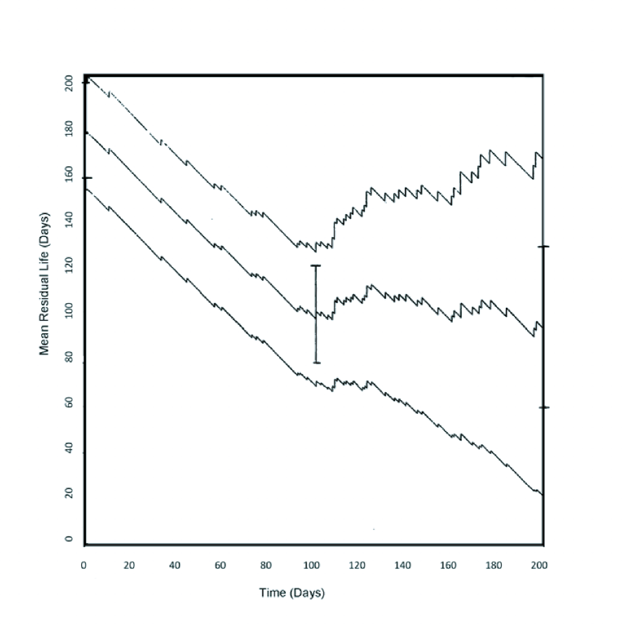
Figure 1: $90\%$ confidence bands for mean residual life; Regimen 4.3

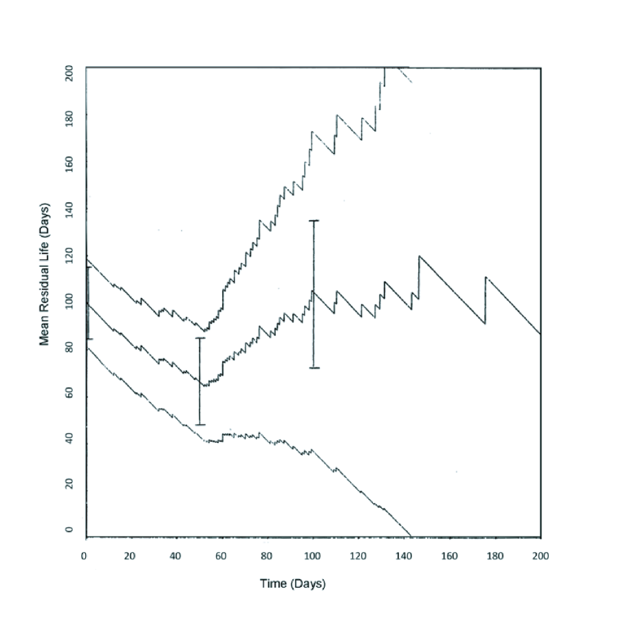
Figure 2: $90\%$ confidence bands for mean residual life; Regimen 6.6

7 Further developments

The original version of this paper, Hall and Wellner [1979], ended with a one-sentence sketch of two remaining problems: “Confidence bands on the difference between two mean residual life functions, and for the case of censored data, will be presented in subsequent papers.” Although we never did address these questions ourselves, others took up these further problems.

Our aim in this final section is to briefly survey some of the developments since 1979 concerning mean residual life, including related studies of median residual life and other quantiles, as well as developments for censored data, alternative inference strategies, semiparametric models involving mean or median residual life, and generalizations to higher dimensions. For a review of further work up to 1988 see Guess and Proschan [1988].

7.1 Confidence bands and inference

Csörgő et al. [1986] gave a further detailed study of the asymptotic behavior of the mean residual life process as well as other related processes including the Lorenz curve. Berger et al. [1988] developed tests and confidence sets for comparing two mean residual life functions based on independent samples from the respective populations. These authors also gave a brief treatment based on comparison of median residual life, to be discussed in Subsection 7.3 below. Csörgő and Zitikis [1996] introduced weighted metrics into the study of the asymptotic behavior of the mean residual life process, thereby avoiding the intervals $[0,x_{n}]$ changing with $n$ involved in our Theorems 2.1 and 2.2, and thereby provided confidence bands and intervals for $e_{F}$ in the right tail. Zhao and Qin [2006] introduced empirical likelihood methods to the study of the mean residual life function. They obtained confidence intervals and confidence bands for compact sets $[0,\tau]$ with $\tau<\tau_{F}\equiv\inf\{x:F(x)=1\}$.

7.2 Censored data

Yang [1978a] initiated the study of estimated mean residual life under random right censorship. She used an estimator $\hat{F}_{n}$ which is asymptotically equivalent to the Kaplan - Meier estimator and considered, in particular, the case when $X$ is bounded and stochastically smaller than the censoring variable $C$. In this case she proved that $\sqrt{n}(\hat{e}(x)-e(x))$ converges weakly (as $n\rightarrow\infty$) to a Gaussian process with mean zero. Csörgő and Zitikis [1996] give a brief review of the challenges involved in this problem; see their page 1726. Qin and Zhao [2007] extended their earlier study (Zhao and Qin [2006]) of empirical likelihood methods to this case, at least for the problem of obtaining pointwise confidence intervals. The empirical likelihood methods seem to have superior coverage probability properties in comparison to the Wald type intervals which follow from our Proposition 5.2. Chaubey and Sen [1999] introduced smooth estimates of mean residual life in the uncensored case. In Chaubey and Sen [2008] they introduce and study smooth estimators of $e_{F}$ based on corresponding smooth estimators of $\overline{F}=1-F$ introduced by Chaubey and Sen [1998].

7.3 Median and quantile residual life functions

Because mean residual life is frequently difficult, if not impossible, to estimate in the presence of right-censoring, it is natural to consider surrogates for it which do not depend on the entire right tail of $F$. Natural replacements include median residual life and corresponding residual life quantiles. The study of median residual life was apparently initiated in Schmittlein and Morrison [1981]. Characterization issues and basic properties have been investigated by Gupta and Langford [1984], Joe and Proschan [1984b], and Lillo [2005]. Joe and Proschan [1984a] proposed comparisons of two populations based on their corresponding median (and other quantile) residual life functions. As noted by Joe and Proschan, “Some results differ notably from corresponding results for the mean residual life function”. Jeong et al. [2008] investigated estimation of median residual life with right-censored data for one-sample and two-sample problems. They provided an interesting illustration of their methods using a long-term follow-up study (the National Surgical Adjuvant Breast and Bowel Project, NSABP) involving breast cancer patients.

7.4 Semiparametric models for mean and median residual life

Oakes and Dasu [1990] investigated a characterization related to a proportional mean residual life model: $e_{G}=\psi e_{F}$ with $\psi>0$. Maguluri and Zhang [1994] studied several methods of estimation in a semiparametric regression version of the proportional mean residual life model, $e(x|z)=\exp(\theta^{T}z)e_{0}(x)$ where $e(x|z)$ denotes the conditional mean residual life function given $Z=z$. Chen et al. [2005] provide a nice review of various models and study estimation in the same semiparametric proportional mean residual life regression model considered by Maguluri and Zhang [1994], but in the presence of right censoring. Their proposed estimation method involves inverse probability of censoring weighted (IPCW) estimation methods (Horvitz and Thompson [1952]; Robins and Rotnitzky [1992]). Chen and Cheng [2005] use counting process methods to develop alternative estimators for the proportional mean residual life model in the presence of right censoring. The methods of estimation considered by Maguluri and Zhang [1994], Chen et al. [2005], and Chen and Cheng [2005] are apparently inefficient. Oakes and Dasu [2003] consider information calculations and likelihood based estimation in a two-sample version of the proportional mean residual life model. Their calculations suggest that certain weighted ratio-type estimators may achieve asymptotic efficiency, but a definitive answer to the issue of efficient estimation apparently remains unresolved. Chen and Cheng [2006] proposed an alternative additive semiparametric regression model involving mean residual life. Ma and Yin [2010] considered a large family of semiparametric regression models which includes both the additive model proposed by Chen and Cheng [2006] and the proportional mean residual life model considered by earlier authors, but advocated replacing mean residual life by median residual life. Gelfand and Kottas [2003] also developed a median residual life regression model with additive structure and took a semiparametric Bayesian approach to inference.

7.5 Monotone and Ordered mean residual life functions

Kochar et al. [2000] consider estimation of $e_{F}$ subject to the shape restrictions that $e_{F}$ is increasing or decreasing. The main results concern ad-hoc estimators that are simple monotizations of the basic nonparametric empirical estimators $\hat{e}_{n}$ studied here. These authors show that the nonparametric maximum likelihood estimator does not exist in the increasing MRL case and that although the nonparametric MLE exists in the decreasing MRL case, the estimator is difficult to compute. Ebrahimi [1993] and Hu et al. [2002] study estimation of two mean residual life functions $e_{F}$ and $e_{G}$ in one- and two-sample settings subject to the restriction $e_{F}(x)\leq e_{G}(x)$ for all $x$. Hu et al. [2002] also develop large sample confidence bands and intervals to accompany their estimators.

7.6 Bivariate residual life

Jupp and Mardia [1982] defined a multivariate mean residual life function and showed that it uniquely determines the joint multivariate distribution, extending the known univariate result of Cox [1962]; see Hall and Wellner [1981] for a review of univariate results of this type. See Ma [1996, 1998] for further multivariate characterization results. Kulkarni and Rattihalli [2002] introduced a bivariate mean residual life function and propose natural estimators.

Remarks: This revision was accomplished jointly by the authors in 2011 and 2012. The first author passed away in October 2012. Section 7 only covers further developments until 2012. A MathSciNet search for “mean residual life” over the period 2011 - 2017 yielded 148 hits on 10 July 2017.

References

- Balkema and de Haan [1974] Balkema, A. A. and de Haan, L. (1974). Residual life time at great age. Ann. Probability, 2, 792–804.
- Barlow and Campo [1975] Barlow, R. E. and Campo, R. (1975). Total time on test processes and applications to failure data analysis. In Reliability and fault tree analysis (Conf., Univ. California, Berkeley, Calif., 1974), pages 451–481. Soc. Indust. Appl. Math., Philadelphia, Pa.
- Berger et al. [1988] Berger, R. L., Boos, D. D., and Guess, F. M. (1988). Tests and confidence sets for comparing two mean residual life functions. Biometrics, 44(1), 103–115.
- Billingsley [1968] Billingsley, P. (1968). Convergence of probability measures. John Wiley & Sons Inc., New York.
- Bjerkedal [1960] Bjerkedal, T. (1960). Acquisition of resistance in guinea pigs infected with different doses of virulent tubercle bacilli. Amer. Jour. Hygiene, 72, 130–148.
- Bryson and Siddiqui [1969] Bryson, M. C. and Siddiqui, M. M. (1969). Some criteria for aging. J. Amer. Statist. Assoc., 64, 1472–1483.
- Chaubey and Sen [2008] Chaubey, Y. P. and Sen, A. (2008). Smooth estimation of mean residual life under random censoring. In Beyond parametrics in interdisciplinary research: Festschrift in honor of Professor Pranab K. Sen, volume 1 of Inst. Math. Stat. Collect., pages 35–49. Inst. Math. Statist., Beachwood, OH.
- Chaubey and Sen [1998] Chaubey, Y. P. and Sen, P. K. (1998). On smooth estimation of hazard and cumulative hazard functions. In Frontiers in probability and statistics (Calcutta, 1994/1995), pages 91–99. Narosa, New Delhi.
- Chaubey and Sen [1999] Chaubey, Y. P. and Sen, P. K. (1999). On smooth estimation of mean residual life. J. Statist. Plann. Inference, 75(2), 223–236. The Seventh Eugene Lukacs Conference (Bowling Green, OH, 1997).
- Chen and Cheng [2005] Chen, Y. Q. and Cheng, S. (2005). Semiparametric regression analysis of mean residual life with censored survival data. Biometrika, 92(1), 19–29.
- Chen and Cheng [2006] Chen, Y. Q. and Cheng, S. (2006). Linear life expectancy regression with censored data. Biometrika, 93(2), 303–313.
- Chen et al. [2005] Chen, Y. Q., Jewell, N. P., Lei, X., and Cheng, S. C. (2005). Semiparametric estimation of proportional mean residual life model in presence of censoring. Biometrics, 61(1), 170–178.
- Chiang [1960] Chiang, C. L. (1960). A stochastic study of the life table and its applications: I. probability distributions of the biometric functions. Biometrics, 16, 618–635.
- Chiang [1968] Chiang, C. L. (1968). Introduction to Stochastic Processes in Biostatistics. Wiley, New York.
- Cox [1962] Cox, D. R. (1962). Renewal theory. Methuen & Co. Ltd., London.
- Csörgő and Zitikis [1996] Csörgő, M. and Zitikis, R. (1996). Mean residual life processes. Ann. Statist., 24(4), 1717–1739.
- Csörgő et al. [1986] Csörgő, M., Csörgő, S., and Horváth, L. (1986). An asymptotic theory for empirical reliability and concentration processes, volume 33 of Lecture Notes in Statistics. Springer-Verlag, Berlin.
- Ebrahimi [1993] Ebrahimi, N. (1993). Estimation of two ordered mean residual lifetime functions. Biometrics, 49(2), 409–417.
- Gelfand and Kottas [2003] Gelfand, A. E. and Kottas, A. (2003). Bayesian semiparametric regression for median residual life. Scand. J. Statist., 30(4), 651–665.
- Gross and Clark [1975] Gross, A. J. and Clark, V. A. (1975). Survival distributions: reliability applications in the biomedical sciences. Wiley, New York.
- Guess and Proschan [1988] Guess, F. and Proschan, F. (1988). Mean residual life: theory and application. In Handbook of Statistics: Quality Control and Reliability, volume 7, pages 215–224. North-Holland, Amsterdam.
- Gupta and Langford [1984] Gupta, R. C. and Langford, E. S. (1984). On the determination of a distribution by its median residual life function: a functional equation. J. Appl. Probab., 21(1), 120–128.
- Hall and Wellner [1981] Hall, W. J. and Wellner, J. (1981). Mean residual life. In Statistics and related topics (Ottawa, Ont., 1980), pages 169–184. North-Holland, Amsterdam.
- Hall and Wellner [1979] Hall, W. J. and Wellner, J. A. (1979). Estimation of mean residual life. Technical report, University of Rochester.
- Hollander and Proschan [1975] Hollander, M. and Proschan, F. (1975). Tests for the mean residual life. Biometrika, 62(3), 585–593.
- Horvitz and Thompson [1952] Horvitz, D. G. and Thompson, D. J. (1952). A generalization of sampling without replacement from a finite universe. J. Amer. Statist. Assoc., 47, 663–685.
- Hu et al. [2002] Hu, X., Kochar, S. C., Mukerjee, H., and Samaniego, F. J. (2002). Estimation of two ordered mean residual life functions. J. Statist. Plann. Inference, 107(1-2), 321–341. Statistical inference under inequality constraints.
- Jeong et al. [2008] Jeong, J.-H., Jung, S.-H., and Costantino, J. P. (2008). Nonparametric inference on median residual life function. Biometrics, 64(1), 157–163, 323–324.
- Joe and Proschan [1984a] Joe, H. and Proschan, F. (1984a). Comparison of two life distributions on the basis of their percentile residual life functions. Canad. J. Statist., 12(2), 91–97.
- Joe and Proschan [1984b] Joe, H. and Proschan, F. (1984b). Percentile residual life functions. Oper. Res., 32(3), 668–678.
- Jupp and Mardia [1982] Jupp, P. E. and Mardia, K. V. (1982). A characterization of the multivariate Pareto distribution. Ann. Statist., 10(3), 1021–1024.
- Kochar et al. [2000] Kochar, S. C., Mukerjee, H., and Samaniego, F. J. (2000). Estimation of a monotone mean residual life. Ann. Statist., 28(3), 905–921.
- Kulkarni and Rattihalli [2002] Kulkarni, H. V. and Rattihalli, R. N. (2002). Nonparametric estimation of a bivariate mean residual life function. J. Amer. Statist. Assoc., 97(459), 907–917.
- Lillo [2005] Lillo, R. E. (2005). On the median residual lifetime and its aging properties: a characterization theorem and applications. Naval Res. Logist., 52(4), 370–380.
- Ma [1996] Ma, C. (1996). Multivariate survival functions characterized by constant product of mean remaining lives and hazard rates. Metrika, 44(1), 71–83.
- Ma [1998] Ma, C. (1998). Characteristic properties of multivariate survival functions in terms of residual life distributions. Metrika, 47(3), 227–240.
- Ma and Yin [2010] Ma, Y. and Yin, G. (2010). Semiparametric median residual life model and inference. Canad. J. Statist., 38(4), 665–679.
- Maguluri and Zhang [1994] Maguluri, G. and Zhang, C.-H. (1994). Estimation in the mean residual life regression model. J. Roy. Statist. Soc. Ser. B, 56(3), 477–489.
- Oakes and Dasu [1990] Oakes, D. and Dasu, T. (1990). A note on residual life. Biometrika, 77(2), 409–410.
- Oakes and Dasu [2003] Oakes, D. and Dasu, T. (2003). Inference for the proportional mean residual life model. In Crossing boundaries: statistical essays in honor of Jack Hall, volume 43 of IMS Lecture Notes Monogr. Ser., pages 105–116. Inst. Math. Statist., Beachwood, OH.
- Qin and Zhao [2007] Qin, G. and Zhao, Y. (2007). Empirical likelihood inference for the mean residual life under random censorship. Statist. Probab. Lett., 77(5), 549–557.
- Robins and Rotnitzky [1992] Robins, J. M. and Rotnitzky, A. (1992). Recovery of information and adjustment for dependent censoring using surrogate markers. In AIDS Epidemiology, Methodological Issues, pages 297–331. Birkhauser, Boston.
- Schmittlein and Morrison [1981] Schmittlein, D. C. and Morrison, D. G. (1981). The median residual lifetime: a characterization theorem and an application. Oper. Res., 29(2), 392–399.
- Shorack [1972] Shorack, G. R. (1972). Functions of order statistics. Ann. Math. Statist., 43, 412–427.
- Shorack and Wellner [1986] Shorack, G. R. and Wellner, J. A. (1986). Empirical Processes with Applications to Statistics. Wiley Series in Probability and Mathematical Statistics: Probability and Mathematical Statistics. John Wiley & Sons Inc., New York.
- Wellner [1977] Wellner, J. A. (1977). A Glivenko-Cantelli theorem and strong laws of large numbers for functions of order statistics. Ann. Statist., 5(3), 473–480.
- Wellner [1978] Wellner, J. A. (1978). Limit theorems for the ratio of the empirical distribution function to the true distribution function. Z. Wahrsch. Verw. Gebiete, 45(1), 73–88.
- Wilson [1938] Wilson, E. B. (1938). The standard deviation of sampling for life expectancy. J. Amer. Statist. Assoc., 33, 705–708.
- Yang [1978a] Yang, G. (1978a). Life expectancy under random censorship. Stochastic Processes Appl., 6(1), 33–39.
- Yang [1978b] Yang, G. L. (1978b). Estimation of a biometric function. Ann. Statist., 6(1), 112–116.
- Zhao and Qin [2006] Zhao, Y. and Qin, G. (2006). Inference for the mean residual life function via empirical likelihood. Comm. Statist. Theory Methods, 35(4-6), 1025–1036.