Origin of the $1/f^{\alpha}$-Spectral-Noise in Chaotic and Regular Quantum Systems

Abstract

Based on the connection between the spectral form factor and the probability to return, the origin of the $1/f^{\alpha}$-noise in fully chaotic and fully integrable systems is traced to the quantum interference between invariant manifolds of the classical dynamics and the dimensionality of those invariant manifolds. This connection and the order-to-chaos transition are analyzed in terms of the statistics of Floquet’s quasienergies of a classically chaotic driving non-linear system. An immediate prediction of the connection established here is that in the presence of decoherence, the spectral exponent $\alpha$ takes the same value, $\alpha=2$, for both, fully chaotic and fully integrable systems.

Introduction.—Quantum systems that in the classical limit are fully chaotic exhibit a variety of universal features Haake (2010) such as level repulsion Bohigas et al. (1984) or, in the semiclassical limit, a non-linear dependence on time of the spectral form factor $K(\tau)$ Hannay and Almeida (1984). These seminal results were obtained on the basis of the predictions of Random Matrix Theory (RMT) Mehta (1991) and ramifications of the Gutzwiller trace formula Gutzwiller (1967, 1971), respectively. Only recently, a connection between these pioneering works was established in context of semiclassical periodic-orbit theory Müler et al. (2004); Heusler et al. (2007).

Based on a time-series perspective, a decade ago, it was discovered and proved that the spectral fluctuations of fully chaotic systems display $1/f$-noise whereas for fully integrable systems, the spectral noise behaves as $1/f^{2}$ Relaño et al. (2002); Gómez et al. (2005); Faleiro et al. (2004). By means of RMT, it is also possible to show that for KAM systems, mixed chaotic systems, chaos-assisted tunnelling Davis and Heller (1981) makes the spectral noise to behave as $1/f^{\alpha}$ with $1<\alpha<2$ Relaño (2008). Therefore, the order-to-chaos transition is fully characterized by the spectral exponent $\alpha$ and contrary to the Dyson $\Delta_{3}(L)$ statistic, the exponent $\alpha$ quantifies the chaoticity of the system in a single parameter. Moreover, $\alpha$ is a natural measure of the fluctuation properties of a quantum system through the power spectrum.

However, having being developed on the basis of RMT, the $1/f^{\alpha}$ behaviour is the result of statistical averages over the probability distribution of the elements of random matrices. Therefore, it is not possible to interpret, e.g., the particular value of $\alpha$ for fully chaotic or integrable systems, in terms of invariant manifolds of the dynamics. Since the average power noise that defines the $1/f^{\alpha}$ behaviour is a function of the spectral form factor $K(\tau)$ (see below), an interpretation is provided here on the basis of recent progress towards the identification of the classical invariant manifolds that contribute to the spectral form factor Dittrich and Pachón (2009). Specifically, by resolving the spectral form factor in phase space, it is shown that the particular value of $\alpha$ for fully chaotic and regular systems can be understood in terms of the dimensionality of the classical invariant manifold of the dynamics (one dimensional for isolated unstable periodic orbits and $N$-dimensional for regular tori) and their coherent quantum interference.

The connection established here permits identifying the different values of the spectral exponent $\alpha$ as a delicate interplay between quantum and classical signatures of the dynamics, namely, quantum interference and the dimensionality of classical invariant structures. The consequences of this connection are manifold, e.g., it predicts that the different value of the spectral exponent for fully chaotic and fully integrable systems doest not survive in the classical limit.

Spectral fluctuations: The average power noise and the spectral form factor.—The fluctuating parts of the level and accumulated level densities are denoted by $\tilde{\rho}(\epsilon)$ and $\tilde{n}(\epsilon)$, respectively. Spectral fluctuations are analyzed in terms of the form factor $K(\tau)$ and the power spectrum $P^{n}(\tau)$, defined as the square modulus of the Fourier transform of $\tilde{\rho}(\epsilon)$ and $\tilde{n}(\epsilon)$, respectively. For $\tau\neq 0$, under the assumptions that $\langle\tilde{\rho}(\epsilon)\tilde{\rho}(\epsilon+\eta)\rangle\rightarrow 0$ faster than $1/\eta$ as $\eta\rightarrow\infty$ and for a large energy window $\Delta E\gg 1$, it can be shown that Faleiro et al. (2004)

$$\frac{\langle|\hat{n}(\tau)|^{2}\rangle}{\Delta E}=\langle P^{n}(\tau)\rangle=\frac{K(\tau)}{4\pi^{2}\tau^{2}},$$ (1)

where $\langle\cdot\rangle$ stands for spectral averages whereas $\hat{\cdot}$ does for Fourier transform of $\tilde{\cdot}$. The program developed in Refs. Relaño et al. (2002); Gómez et al. (2005); Faleiro et al. (2004) aims at introducing a time series perspective to characterize the spectral noise of $\langle P^{n}(\tau)\rangle$. The main idea behind this approach is to consider the sequence of energy levels as a discrete time series and study level correlations using tools from time-series analysis.

Time-series perspective of quantum chaos: The average power noise and the spectral form factor.—The analogy between the energy spectrum and a discrete time series is established in terms of the $\delta_{q}$ statistic Relaño et al. (2002), defined as the deviation of the $(q+1)$-th level from its mean value. In terms of unfolded energy levels $\delta_{q}=\sum_{i=1}^{q}\left(s_{i}-\langle s\rangle\right)=\epsilon_{q+1}-\epsilon_{1}-q,$ where $s_{i}=\epsilon_{i+1}-\epsilon_{i}$, $\epsilon_{i}$ is the $i$-th unfolded level and $\langle s\rangle=1$ is the average value of $s_{i}$.

The unfolded energy levels are defined using the average accumulated level density $\bar{N}(E)$ as $\epsilon_{i}=\bar{N}(E_{i})$. This mapping is needed to remove the main trend defined by the smooth part of the level density and compare between the statistical properties of the spectral fluctuations of different systems or different parts of the same spectrum. In the language of time series analysis, the unfolding mapping is a procedure for making stationary the discrete time series defined by the $\delta_{q}$, its average and fluctuations not depending on time. Sampling $\tilde{n}(\epsilon)$ for integer values of the energy leads to the discrete function $\tilde{n}_{q}(\epsilon)$ with averaged power spectrum $\langle P_{k}^{n}\rangle$ and Fourier transform is given by $\hat{n}_{k}=D_{\mathcal{H}}^{-\frac{1}{2}}\sum_{q=-\infty}^{\infty}\hat{n}\left(k/D_{\mathcal{H}}+q\right)$, with $k=1,2,\ldots,D_{\mathcal{H}}-1$. $D_{\cal{H}}=\Delta E/\langle d\rangle$ is the effective dimension of the Hilbert space ${\cal{H}}$ and $\langle d\rangle$ denotes the mean spectral density for a finite range $\Delta E$. The averaged power noise of $\delta_{k}$ is related to $\langle P_{k}^{n}\rangle$ by $\langle P_{k}^{\delta}\rangle=\langle P_{k}^{n}\rangle-\frac{1}{12}$ for chaotic systems and by $\langle P_{k}^{\delta}\rangle=\langle P_{k}^{n}\rangle$ for regular systems. If $D_{\mathcal{H}}\gg 1$ and $k\ll D_{\mathcal{H}}$, $\langle P_{k}^{\delta}\rangle_{\beta}=D_{\mathcal{H}}/(2\beta\pi^{2}k)$ for chaotic systems belonging to the three $\beta=\{1,2,4\}$ classical RMT (for fully chaotic systems) whereas $\langle P_{k}^{\delta}\rangle=D_{\mathcal{H}}^{2}/(4\pi^{2}k^{2})$ for integrable systems. Thus, for small frequencies, the excitation energy fluctuations exhibit $1/f$ ($\sim 1/k$) noise in chaotic systems and $1/f^{2}$ ($\sim 1/k^{2}$) noise in integrable systems Faleiro et al. (2004).

Interference of time-domain scars: Spectral form factor and probability to return—The key quantity that allows for the identification of the contribution of classical invariant manifolds to $K(\tau)$ is the probability to return $P^{\mathrm{qm}}_{\mathrm{ret}}(t)$ Dittrich and Smilansky (1991); Dittrich (1996); Dittrich and Pachón (2009). To make a clear connection with the classical invariant manifolds of the underlying classical dynamics, it is convenient to express the return probability in terms of phase-space objects. To do so, introduce the Weyl representation of quantum mechanics Weyl (1950), which assigns a phase space function $O(\mathbf{p},\mathbf{q})$ to an operator $\hat{O}$. For the density operator $\hat{\rho}(t)$ at time $t$, the Weyl transform defines the Wigner function $\rho_{\mathrm{W}}(\mathbf{r},t)=\int\mathrm{d}^{N}q^{\prime}\exp(-\mathrm{i}\mathbf{p}\cdot\mathbf{q}^{\prime}/\hbar)\langle\mathbf{q}+\mathbf{q}^{\prime}/2|\hat{\rho}(t)|\mathbf{q}-\mathbf{q}^{\prime}/2\rangle$ with $\mathbf{r}=(\mathbf{p},\mathbf{q})$ a vector in $2N$-dimensional phase-space. The propagator $G_{\mathrm{W}}(\mathbf{r}^{\prime\prime},t^{\prime\prime};\mathbf{r}^{\prime},t^{\prime})$ of the Wigner function evolves the Wigner function from $t^{\prime}$ to $t^{\prime\prime}$, $\rho_{\mathrm{W}}(\mathbf{r}^{\prime\prime},t^{\prime\prime})=\int\mathrm{d}^{2N}rG_{\mathrm{W}}(\mathbf{r}^{\prime\prime},t^{\prime\prime};\mathbf{r}^{\prime},t^{\prime})\rho_{\mathrm{W}}(\mathbf{r}^{\prime},t^{\prime})$ and has a clear classical analog, namely, the Liouville propagator Prigogine (1962).

The quantum probability to return can be expressed as a trace over phase space of the propagator of the Wigner function, namely, $P^{\mathrm{qm}}_{\mathrm{ret}}(t)=\int\mathrm{d}^{2f}r_{0}G_{\mathrm{W}}(\mathbf{r}_{0},t;\mathbf{r}_{0})$, with $t=t^{\prime\prime}-t^{\prime}$. For $t\gtrsim t_{\rm H}/D_{\cal{H}}$, the form factor is related to the quantum return probability by Dittrich and Pachón (2009)

$$D_{\mathcal{H}}K(\tau)=\int\mathrm{d}^{2f}rG_{\mathrm{W}}(\mathbf{r},t;\mathbf{r},0)=P^{\mathrm{qm}}_{\mathrm{ret}}(t),$$ (2)

with $\tau=t/t_{\mathrm{H}}$ and $t_{\rm H}=h\langle d\rangle$ denotes the Heisenberg time. Remarkably, before tracing, the quasiprobability density to return $G_{\mathrm{W}}(\mathbf{r},t;\mathbf{r},0)$ allows for the identification of the manifolds that contributed to the form factor (see Fig. 1 below). At the semiclassical level, besides the classical invariant manifolds with period $T^{\mathrm{p}}$ and invariant manifolds with period $T=T^{\mathrm{p}}/l$, being $l$ and integer, also sets of midpoints between them contribute Dittrich and Pachón (2009). These midpoint manifolds constitute important exceptions from a continuous convergence in the classical limit of the Wigner towards the Liouville propagator Dittrich and Pachón (2009) and, as shown below, are responsible for the different functional form of the spectral noise in chaotic and regular systems.

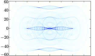
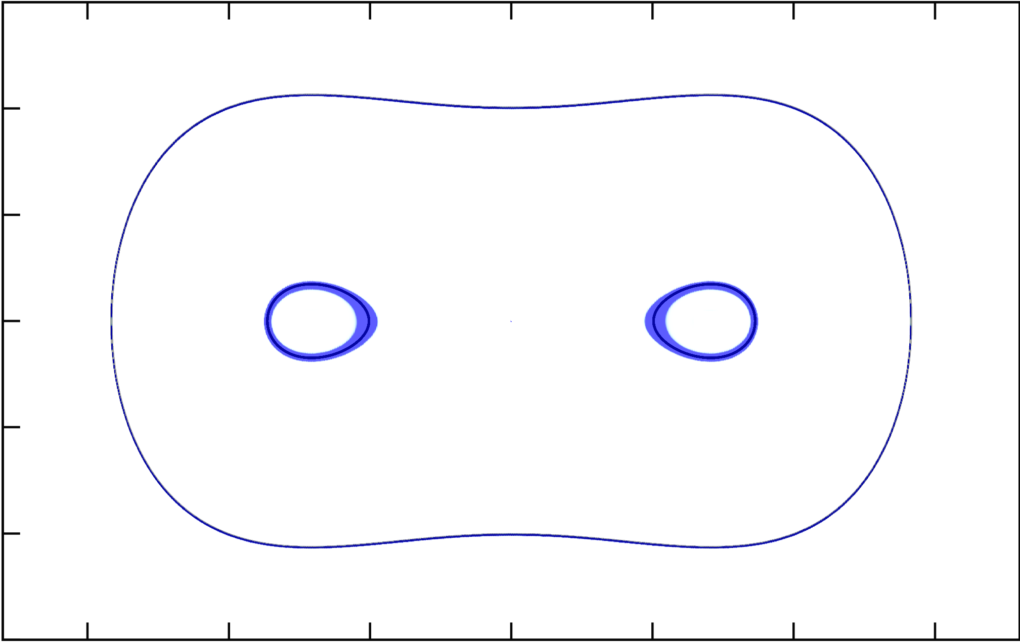
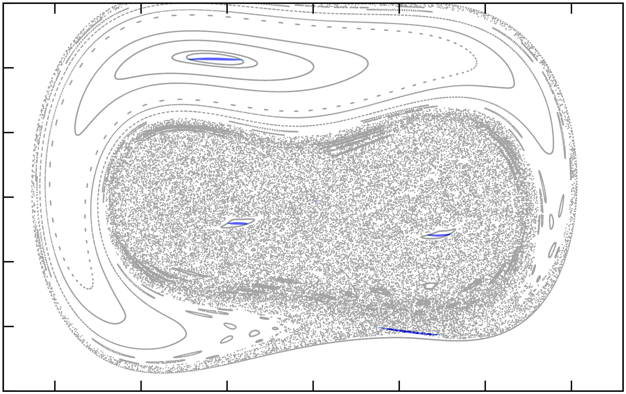
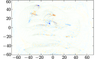
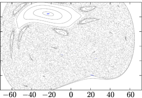
Figure 1: Quantum (l.h.s. panel) and classical (r.h.s. panel) diagonal propagators $G({\bf r},t;{\bf r},0)$ for the harmonically driven quartic oscillator at $t=T\equiv 2\pi/\Omega$, with $\omega_{0}=1.0$, $\Omega=0.95$, $E_{\rm b}=100.0$, $\phi=\pi/3$ with $S=0$ (upper panels), $S=2.5$ (central panels) and $S=10$ (lower panels). For better understanding of the midpoint contributions in the diagonal propagator, Poincare surface of sections are shown behind of the classical diagonal propagator.

Probability to return and the average power noise—The connection between the averaged power-spectrum of the spectral fluctuations and the invariant manifolds of the classical dynamics, and their quantum interferences, is established from the comparison between Eqs. (1) and (2)

$$\langle P^{n}(\tau)\rangle=D_{\mathcal{H}}^{-1}(2\pi\tau)^{-2}P^{\mathrm{qm}}_{\mathrm{ret}}(t)$$ (3)

Because this identity does not rely on any semiclassical approximation, it is exact and holds for finite- and infinite-dimensional Hilbert spaces. Moreover, because it is formulated at the level of the statistical operator $\hat{\rho}$ and not at the level of elements of the projective Hilbert space, it holds for unitary as well as non-unitary dynamics.

As stated above, the calculation of $\langle P_{k}^{\delta}\rangle$ requieres the unfolding of the energy leves. Here, that unfolding needs to be reinterpreted and calculated at the level of the return probability, which is defined as a direct trace over phase space of the diagonal propagator $G_{\mathrm{W}}(\mathbf{r},t;\mathbf{r},0)$. Thus, the subtraction of the main trend translates here into to the subtraction of the classical contribution, i.e., it is assumed that the quantum propagator can be accounted for by the superposition of the classical propagator plus quantum fluctuations Dittrich et al. (2006); Dittrich and Pachón (2009); Dittrich et al. (2010); Pachón et al. (2010). Thus, define the quantities $\Delta P_{\mathrm{ret}}(t)=P^{\mathrm{qm}}_{\mathrm{ret}}(t)-P^{\mathrm{cl}}_{\mathrm{ret}}(t)$ and $\langle\Delta P^{n}(\tau)\rangle=D_{\mathcal{H}}^{-1}(2\pi\tau)^{-2}\Delta P_{\mathrm{ret}}(t)$. In the semiclassical limit,

$$P^{\mathrm{qm}}_{\mathrm{ret}}(t)\approx\begin{cases}D_{\mathcal{H}}(2/\beta)\tau P^{\mathrm{cl}}_{\mathrm{ret}}(t),&\mathrm{for\,fully\,chaotic\,systems},\\ D_{\mathcal{H}}P^{\mathrm{cl}}_{\mathrm{ret}}(t),&\mathrm{for\,integrable\,systems},\end{cases}$$ (4)

where no degeneracies are considered for the integrable case Dittrich (1996). So that, for $D_{\mathcal{H}}\gg 1$,

$$\frac{\langle\Delta P^{n}(\tau)\rangle}{P^{\mathrm{cl}}_{\mathrm{ret}}(t)}\approx\begin{cases}(2\pi^{2}\beta)^{-1}\tau^{-1},&\mathrm{for\,fully\,chaotic\,systems},\\ (4\pi^{2})^{-1}\tau^{-2},&\mathrm{for\,integrable\,systems}.\end{cases}$$ (5)

$\langle\Delta P^{n}(\tau)\rangle/P^{\mathrm{cl}}_{\mathrm{ret}}(t)$ measures deviations from the main trend, classical contributions, normalized by the classical return probability. From Eq. (5), it is clear that the description in terms of the return probability provides consistent results with the time-series perspective developed in Refs. Relaño et al. (2002); Gómez et al. (2005); Faleiro et al. (2004), i.e., deviations of the averaged power spectrum from the main trend behave as $1/\tau^{\alpha}$ with $\alpha=1$ for chaotic and $\alpha=2$ for integrable systems, respectively. The results formally coincides after, as defined above, replacing $\tau$ by $k/D_{\mathcal{H}}$ .

The main advantage of the present formulation relies on the possibility of interpreting the origin of the different values of the exponent $1\leq\alpha\leq 2$. As shown above, the different nature of the spectral noise relies on the particular functional dependence of the quantum return probability on $\tau$ [see Eq. (4)]. Therefore, this particular dependence relies on the different nature of classical invariant manifolds that contribute to the quantum return probability Dittrich and Pachón (2009). Specifically, it is understood in terms of midpoints manifolds showing up from the interference of periodic invariants of the dynamics (see, e.g., Fig. 1 and description below). For regular systems, the number and size of these manifolds scale with time the same way as that of the underlying tori Hannay and Almeida (1984); Dittrich and Pachón (2009), so that no $\tau$ factor arises between quantum and classical return probabilities in Eq. (4). This situation in turn reflects the fact that periodic tori form $N$-dimensional surfaces in phase space and are space filling, e.g., in position space. In contrast, isolated periodic orbits remain one-dimensional subsets independently of the number of freedoms, this dimensionality property is in turn responsible for the emergence of the $\tau$ factor for fully chaotic systems Dittrich and Pachón (2009). There is therefore qualitatively “more room” available for midpoint manifolds in the latter case than in the former.

Example—Traditionally, the study of spectral fluctuations have been performed in nuclear systems or 2D billiards Relaño et al. (2002); Gómez et al. (2005); Faleiro et al. (2004). However, because the dimension of the Wigner propagator is four times the real space dimension, a phase-space characterization of the invariant manifolds in this object is not feasible for those systems. For this reason, a one-dimensional driven mixed chaotic systems, prototypical in, e.g., coherent destruction of tunnelling Grossmann et al. (1991), is considered here, namely, $H=p^{2}/2m-m\omega^{2}q^{2}/4+m^{2}\omega^{4}q^{4}/64E_{\mathrm{b}}+S\cos(\Omega t+\phi)$. $E_{\mathrm{b}}$ denotes, roughly, the number of tunnelling doublets and $S$ stands for the strength of the driving force.

Because of the periodicity of the driving force, spectral fluctuations are analyzed for Floquet’s quasienergies, that are eigenvalues of the unitary-time evolution operator $\hat{U}(t)$ over one period of driving $T=2\pi/\Omega$. To the best of our knowledge, this is the first time that a characterization of the spectral noise is performed for a driven mixed chaotic systems and thus, some comments are in order. The unitarity of the time-evolution operator implies that its eigenvalues are of unit magnitude and therefore, they can be conveniently written as $\exp(\mathrm{i}E_{\alpha}T/\hbar)$, being $E_{\alpha}$ Floquet’s quaisenergies. $E_{\alpha}$ is defined modulo integer multiples of $\hbar\Omega$, namely, $E_{\alpha}=E_{n,l}=E_{n,0}+l\hbar\Omega$, $n=0,1,2,...$ and $l=0,\pm 1,\pm 2,...$

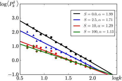
Figure 2: Theoretical power spectrum of the $\delta_{q}$ function. Parameter values are as in Fig. 1.

For the spectral statistics, only the quasienergies in the first Brillouin’s zone, $l=0$, are considered, so that $-\hbar\Omega<E_{n}<\hbar\Omega$.

Before discussing the spectral features of this system, it is instrumental to have a qualitatively idea about the underlying manifolds that will determined the spectral exponent $\alpha$. Figure 1 depicts the quantum quasi-probability density $G_{\mathrm{W}}(\mathbf{r},t,\mathbf{r},0)$ for the driven doble well potential considered above for zero driving ($S=0$, upper panel), strong driving ($S=2.5$, central panel) and ultra strong driving ($S=10$, lower panel). For the classical dynamics of the undriven case, there exists three periodic orbits of period $T$ that can be clearly seen in the diagonal classical propagator (l.h.s. of Fig. 1). Thee is also a family of orbits whose period is a rational fraction of $T$, e.g., $T/2$, that is located outside of the domain of the plot. The interference of these manifold is clearly visible in the upper panel of Fig. 1. In the presence of driving, these continuous manifold are replaced by a set of unstable elliptical and hyperbolic periodic points (see central and lower panels in in Fig. 1). Remarkably, the quantum interference between these manifold (contributions from midpoints between classical invariant manifolds) is also clearly visible in the central and lower panels of Fig. 1.

Figure 2 depicts the functional dependence of $\langle P^{\delta}_{k}\rangle$ on $k$ for Floquet’s quasienergies for $S=0$ ($\alpha=1.99$), $S=2.5$ ($\alpha=1.71$), $S=10$ ($\alpha=1.29$) and $S=100$ ($\alpha=1.13$). Despite the KAM nature of the system at hand, the spectral fluctuations exhibit a clear $1/f^{\alpha}$ dependence. This feature of Floquet’s quasienergies supports the evidence found in the Robnik billiard Gómez et al. (2005), and are in sharp contrast to the conventional expectation that in the strict semiclassical limit spectral fluctuations of mixed chaotic systems cannot follow a power law Gómez et al. (2005); Relaño (2008).

Discussion—In this Letter, by establishing a connection between the power noise and the probability to return [see Eqs. (3, 5)], the origin of the $1/f^{\alpha}$ noise in quantum systems (for $\alpha=1,2$) was track to the interference and dimensionality of classical invariant manifolds of the regular and chaotic dynamics. In the process, the main trend of the power spectrum was associated to the classical contribution to the quantum dynamics, so that $\langle\Delta P^{n}(\tau)\rangle/P^{\mathrm{cl}}_{\mathrm{ret}}(t)$ measures purely quantum fluctuations.

The extreme values of the $\alpha$ parameter, $\alpha=1$ and $\alpha=2$, are the result of the $\tau$ dependence of the quantum return probability [see, Eq. (4)]. Because the connections stablished above are valid in general, it suggest that the fractional behaviour of the spectral noise, $1<\alpha<2$ emerges for the interference between regular and chaotic invariant manifolds, however, an analytic account of this fact remains as a challenge.

This same connection allows for the immediate prediction that in the presence of decoherence, the spectral coefficient $\alpha$ takes the same value, $\alpha=2$, for classically chaotic and classically regular systems. This follows from the fact that in the presence of decoherence, the quantum return probability behaves equally for both, integrable and chaotic systems Braun (1999). In a nutshell, decoherence removes the interference between invariant manifolds so that the additional coherent contributions to the form factor discovered in Ref. Dittrich and Pachón (2009) are not present anymore. Work along this line will be reported soon Pachon et al. (2017).

The approach presented here can be extended to uncover the invariant manifolds responsible for the behaviour of the power spectrum of energy level fluctuations very recently discussed in the nonperturbative analysis of the in fully chaotic quantum structures was reported Riser et al. (2017).