Searching for left sneutrino LSP at the LHC

Abstract

We analyze relevant signals expected at the LHC for a left sneutrino as the lightest supersymmetric particle (LSP). The discussion is carried out in the ‘$\mu$ from $\nu$’ supersymmetric standard model ($\mu\nu{\rm SSM}$), where the presence of $R$-parity breaking couplings involving right-handed neutrinos solves the $\mu$ problem and reproduces neutrino data. The sneutrinos are pair produced via a virtual $W$, $Z$ or $\gamma$ in the $s$ channel. From the prompt decay of a pair of left sneutrinos LSPs of any family, a significant diphoton signal plus missing transverse energy (MET) from neutrinos can be present in the mass range 118–132 GeV, with 13 TeV center-of-mass energy and an integrated luminosity of 100 fb^-1. In addition, in the case of a pair of tau left sneutrinos LSPs, given the large value of the tau Yukawa coupling diphoton plus leptons and/or multileptons can appear. We find that the number of expected events for the multilepton signal, together with properly adopted search strategies, is sufficient to give a significant evidence for a sneutrino of mass in the range 130–310 GeV, even with the integrated luminosity of 20 fb^-1. In the case of the signal producing diphoton plus leptons, an integrated luminosity of 100 fb^-1 is needed to give a significant evidence in the mass range 95–145 GeV. Finally, we discuss briefly the presence of displaced vertices and the associated range of masses.

1 Introduction

In supersymmetry (SUSY), the ‘$\mu$ from $\nu$’ supersymmetric standard model ($\mu\nu$SSM LopezFogliani:2005yw ; Escudero:2008jg , see Refs. Munoz:2009an ; Munoz:2016vaa for reviews) is a natural extension of the minimal supersymmetric standard model (MSSM, see Ref. Martin:1997ns for a review), since only trilinear couplings involving right-handed neutrino superfields, $\hat{\nu}^{c}_{i}$ with $i=1,2,3$, are added to the superpotential. Thus, in addition to the usual Dirac Yukawa couplings for neutrinos $Y^{\nu}_{ij}\,\hat{H}_{u}\,\hat{L}_{i}\,\hat{\nu}^{c}_{j}$, other two types of couplings can be present by gauge invariance solving crucial problems of the MSSM. In particular, the couplings between the three families of right-handed neutrino and Higgs superfields, $\lambda_{i}\,\hat{\nu}^{c}_{i}\,\hat{H}_{d}\hat{H}_{u}$, generate an effective $\mu$ term solving the so-called $\mu$ problem Kim:1983dt . This occurs when the SUSY partners of the right-handed neutrinos, the right sneutrinos $\tilde{\nu}_{iR}$, develop vacuum expectation values (VEVs) after the successful electroweak symmetry breaking (EWSB), with the result $\mu^{\text{eff}}=\lambda_{i}\langle\widetilde{\nu}_{iR}\rangle$*. Besides, the couplings among right-handed neutrino superfields, $\frac{1}{3}\kappa{{}_{ijk}}\hat{\nu}^{c}_{i}\hat{\nu}^{c}_{j}\hat{\nu}^{c}_{k}$, generate effective Majorana masses for right-handed neutrinos of the order of the EWSB scale, $\left(m^{\text{eff}}_{\mathcal{M}}\right)_{ij}={2}\kappa_{ijk}\langle\widetilde{\nu}_{kR}\rangle$*, instrumental in solving the $\nu$ problem, i.e. the generation of neutrino masses and mixing in SUSY. The solution is obtained through a generalized electroweak-scale seesaw mechanism, involving also the neutralinos, that can accommodate the correct neutrino data with $Y^{\nu}_{ij}\raise 1.29167pt\hbox{$\;<$\kern-7.5pt\raise-4.73611pt\hbox{$\sim\;$}}10^{-6}$ LopezFogliani:2005yw ; Escudero:2008jg ; Ghosh:2008yh ; Bartl:2009an ; Fidalgo:2009dm ; Ghosh:2010zi (see Refs. LopezFogliani:2010bf ; Ghosh:2010ig for reviews).

Both types of couplings discussed above, determined by $\lambda_{i}$ and $\kappa_{ijk}$, break explicitly $R$ parity ($R_{p}$). Nevertheless, in the limit $Y^{\nu}_{ij}\to 0$, $\hat{\nu}^{c}_{i}$ can be identified as pure singlet superfields without lepton number and $R_{p}$ is not broken. Therefore, $Y^{\nu}_{ij}$ are the parameters determining the violation of $R$ parity (${R}_{p}/\hskip 5.69046pt$), and as a consequence such violation is small in the $\mu\nu{\rm SSM}$. As is well known, in models with ${R}_{p}/\hskip 5.69046pt$ the LSP is not stable, decaying into standard model (SM) particles, and basically all SUSY particles (sparticles) are potential candidates for LSPs, not only the neutral ones as in $R_{p}$ conserving models where they are stable and therefore contribute to the dark matter. This means that in the $\mu\nu{\rm SSM}$, squarks, gluinos, sleptons, sneutrinos, neutralinos and charginos, are potential candidates for LSPs. Therefore, an analysis of the LHC phenomenology associated to each candidate is crucial to test the model.

In this work we start with the systematic analysis of relevant signals expected at the LHC for LSP candidates in the $\mu\nu{\rm SSM}$. As a first candidate we will concentrate on the SUSY partner of the left-handed neutrino, the left sneutrino, studying in particular its dominant pair production channels and decays. It is worth noticing here that in $R_{p}$ conserving models where the left sneutrino LSP is stable and therefore contributes to thermal dark matter Ibanez:1983kw ; Hagelin:1984wv , is ruled out by direct detection experiments Falk:1994es ; Arina:2007tm . For proposals to revive it through the breaking of lepton number or inspired in extra dimensions/gauge mediation, see e.g. Refs. Hall:1997ah and Chala:2017jgg , respectively. If the left sneutrino is not the LSP, then the invisible width of the $Z$ puts a lower limit on its mass of about 45 GeV. Also, under the assumption of gaugino and sfermion mass universality at the GUT scale in the MSSM, searches for gauginos and sleptons give rise to a lower limit of about 94 GeV Abdallah:2003xe .

Related to what was discussed before, although the LSP is not stable in the $\mu\nu{\rm SSM}$, SUSY candidates for dark matter exist in models with ${R}_{p}/\hskip 5.69046pt$. This is in particular the case of the gravitino Borgani:1996ag ; Takayama:2000uz . Although it decays into SM particles as any other LSP, its lifetime can be longer than the age of the Universe since the decay width is suppressed both by the inverse of the Planck mass and by the ${R}_{p}/\hskip 5.69046pt$ parameters. The latter are very small in the $\mu\nu{\rm SSM}$, since they are set by the neutrino Yukawa couplings $Y^{\nu}_{ij}\raise 1.29167pt\hbox{$\;<$\kern-7.5pt\raise-4.73611pt\hbox{$\sim\;$}}10^{-6}$. Searches for $\mu\nu{\rm SSM}$ gravitino dark matter in Fermi-LAT data through gamma-ray lines have been carried out in Refs. Choi:2009ng ; GomezVargas:2011ph ; Albert:2014hwa ; Gomez-Vargas:2016ocf , obtaining stringent constraints on the gravitino mass and the lifetime. It is worth noticing that since the gravitino is assumed to be the LSP in this framework, each candidate for LSP mentioned above would in fact be the next-to-LSP (NLSP). Nevertheless, the analysis of their phenomenology at the LHC is not altered, since they also decay into ordinary particles using the same channels as if they were the LSP. Thus the results of this work can also be applied to the case of a left sneutrino NLSP, with the gravitino as the LSP.

The paper is organized as follows. In Section 2, the main characteristics of the $\mu\nu{\rm SSM}$ useful for our computation are briefly discussed. In Section 3, the spectrum of the model is analyzed, paying special attention to the neutral fermion mass matrix which determines neutrino masses and mixing. In Section 4, we analyze in detail how the left sneutrino can become the LSP in some regions of the parameter space of the model, defining at the same time several interesting benchmark points (BPs). In particular, we study points with a left sneutrino LSP of the first two families, and separately points with a left sneutrino LSP of the third family. The different decay modes of the left sneutrino, depending on its nature, scalar or pseudoscalar, are discussed Section 5. In Section 6, we study the dominant pair production channels of sneutrinos at the LHC, as well as the signals. These can consist of a diphoton plus missing transverse energy (from neutrinos), a diphoton plus leptons, and multileptons. For the regions of the parameter space analyzed, we compute the number of expected events for the signals. Given properly modified search techniques, it is sufficient to give a significant evidence with 13 TeV center-of-mass energy using the current or future integrated luminosity, for a sneutrino mass in the range $95-310$ GeV. Our conclusions and prospect for future studies of displaced vertices are presented in Section 7. Finally, a plethora of useful formulae are given in the Appendices. In Appendix A, the superpotential and the associated soft terms of the $\mu\nu{\rm SSM}$ are briefly reviewed and discussed. In Appendix B, the scalar and fermion mass matrices of the model are shown. Finally, in Appendix C, the relevant interactions for the decays of the left sneutrino are obtained.

2 The $\mu\nu{\rm SSM}$

The couplings of the superpotential relevant for this work are given by

$$W= \epsilon_{ab}\left(Y^{e}_{ij}\,\hat{H}_{d}^{a}\,\hat{L}^{b}_{i}\,\hat{e}_{j}^{c}+Y^{d}_{ij}\,\delta_{\alpha\beta}\,\hat{H}_{d}^{a}\,\hat{Q}^{b}_{i\alpha}\,\hat{d}_{j\beta}^{c}+Y^{u}_{ij}\,\delta_{\alpha\beta}\,\hat{H}_{u}^{b}\,\hat{Q}^{a}_{i\alpha}\,\hat{u}_{j\beta}^{c}\right)$$ (1)

$$+ \epsilon_{ab}\left(Y^{\nu}_{ij}\,\hat{H}_{u}^{b}\,\hat{L}^{a}_{i}\,\hat{\nu}^{c}_{j}-\lambda_{i}\,\hat{\nu}^{c}_{i}\,\hat{H}_{u}^{b}\hat{H}_{d}^{a}\right)+\frac{1}{3}\kappa{{}_{ijk}}\hat{\nu}^{c}_{i}\hat{\nu}^{c}_{j}\hat{\nu}^{c}_{k}\ ,$$

as discussed in the Introduction and Appendix A. Together with the corresponding soft SUSY-breaking terms, they give rise to the following tree-level neutral scalar potential:

$$V^{(0)}=V_{\text{soft}}+V_{F}+V_{D}\ ,$$ (2)

with

$$V_{\text{soft}}= \left(T^{\nu}_{ij}\,H_{u}^{0}\,\widetilde{\nu}_{iL}\,\widetilde{\nu}_{jR}^{*}-T^{\lambda}_{i}\,\widetilde{\nu}_{iR}^{*}\,H_{d}^{0}H_{u}^{0}+\frac{1}{3}T^{\kappa}_{ijk}\,\widetilde{\nu}_{iR}^{*}\widetilde{\nu}_{jR}^{*}\widetilde{\nu}_{kR}^{*}\ +\text{h.c.}\right)$$ (3)

$$+ \left(m_{\widetilde{L}_{L}}^{2}\right)_{ij}\widetilde{\nu}_{iL}^{*}\widetilde{\nu}_{jL}+\left(m_{\widetilde{\nu}_{R}}^{2}\right)_{ij}\widetilde{\nu}_{iR}^{*}\widetilde{\nu}_{jR}+m_{H_{d}}^{2}{H^{0}_{d}}^{*}H^{0}_{d}+m_{H_{u}}^{2}{H^{0}_{u}}^{*}H^{0}_{u}\ ,$$

$$V_{F}= \lambda_{j}\lambda_{j}^{*}H^{0}_{d}H_{d}^{0}{{}^{{}^{*}}}H^{0}_{u}H_{u}^{0}{{}^{{}^{*}}}+\lambda_{i}\lambda_{j}^{*}\tilde{\nu}^{*}_{iR}\tilde{\nu}_{jR}H^{0}_{d}H_{d}^{0}{{}^{*}}+\lambda_{i}\lambda_{j}^{*}\tilde{\nu}^{*}_{iR}\tilde{\nu}_{jR}H^{0}_{u}H_{u}^{0}{{}^{*}}$$ (4)

$$+ \kappa_{ijk}\kappa_{ljm}^{*}\tilde{\nu}^{*}_{iR}\tilde{\nu}_{lR}\tilde{\nu}^{*}_{kR}\tilde{\nu}_{mR}-\left(\kappa_{ijk}\lambda_{j}^{*}\tilde{\nu}^{*}_{iR}\tilde{\nu}^{*}_{kR}H_{d}^{0*}H_{u}^{0*}-Y^{\nu}_{ij}\kappa_{ljk}^{*}\tilde{\nu}_{iL}\tilde{\nu}_{lR}\tilde{\nu}_{kR}H^{0}_{u}\right.$$

$$+ \left.Y^{\nu}_{ij}\lambda_{j}^{*}\tilde{\nu}_{iL}H_{d}^{0*}H_{u}^{0*}H^{0}_{u}+{Y^{\nu}_{ij}}^{*}\lambda_{k}\tilde{\nu}_{iL}^{*}\tilde{\nu}_{jR}\tilde{\nu}_{kR}^{*}H^{0}_{d}+\text{h.c.}\right)$$

$$+ Y^{\nu}_{ij}{Y^{\nu}_{ik}}^{*}\tilde{\nu}^{*}_{jR}\tilde{\nu}_{kR}H^{0}_{u}H_{u}^{0}{{}^{*}}+Y^{\nu}_{ij}{Y^{\nu}_{lk}}^{*}\tilde{\nu}_{iL}\tilde{\nu}_{lL}^{*}\tilde{\nu}_{jR}^{*}\tilde{\nu}_{kR}+Y^{\nu}_{ji}{Y^{\nu}_{ki}}^{*}\tilde{\nu}_{jL}\tilde{\nu}_{kL}^{*}H^{0}_{u}H_{u}^{0*}\,,$$

$$V_{D}= \frac{1}{8}\left(g^{2}+g^{\prime 2}\right)\left(\widetilde{\nu}_{iL}\widetilde{\nu}_{iL}^{*}+H^{0}_{d}{H^{0}_{d}}^{*}-H^{0}_{u}{H^{0}_{u}}^{*}\right)^{2}\,.$$ (5)

The electroweak gauge couplings are estimated at the $m_{Z}$ scale by $e=g\sin\theta_{W}=g^{\prime}\cos\theta_{W}$. Since only dimensionless trilinear couplings are present in the superpotential, the EWSB is determined by the soft terms of the scalar potential. Thus all known particle physics phenomenology can be reproduced in the $\mu\nu{\rm SSM}$ with one scale, the about 1 TeV scale of the soft terms, avoiding the introduction of ‘ad-hoc’ high-energy scales. With the choice of CP conservation, one can define the neutral scalars as

$$H_{d}^{0} = \frac{1}{\sqrt{2}}\left(H_{d}^{\mathcal{R}}+v_{d}+i\ H_{d}^{\mathcal{I}}\right)\ ,$$ (6)

$$H^{0}_{u} = \frac{1}{\sqrt{2}}\left(H_{u}^{\mathcal{R}}+v_{u}+i\ H_{u}^{\mathcal{I}}\right)\ ,$$ (7)

$$\widetilde{\nu}_{iR} = \frac{1}{\sqrt{2}}\left(\widetilde{\nu}^{\mathcal{R}}_{iR}+v_{iR}+i\ \widetilde{\nu}^{\mathcal{I}}_{iR}\right),$$ (8)

$$\widetilde{\nu}_{iL} = \frac{1}{\sqrt{2}}\left(\widetilde{\nu}_{iL}^{\mathcal{R}}+v_{iL}+i\ \widetilde{\nu}_{iL}^{\mathcal{I}}\right)\ ,$$ (9)

in such a way that after the EWSB they develop the real VEVs

$$\langle H_{d}^{0}\rangle=\frac{v_{d}}{\sqrt{2}}\ ,\,\quad\langle H_{u}^{0}\rangle=\frac{v_{u}}{\sqrt{2}}\ ,\,\quad\langle\widetilde{\nu}_{iR}\rangle=\frac{v_{iR}}{\sqrt{2}}\ ,\,\quad\langle\widetilde{\nu}_{iL}\rangle=\frac{v_{iL}}{\sqrt{2}}\ .$$ (10)

The eight minimization conditions with respect to $v_{d}$, $v_{u}$, $v_{iR}$ and $v_{iL}$ can then be written as

$$m_{H_{d}}^{2} = -\frac{1}{8}\left(g^{2}+g^{\prime 2}\right)\left(v_{iL}v_{iL}+v_{d}^{2}-v_{u}^{2}\right)-\frac{1}{2}\lambda_{i}\lambda_{j}v_{iR}v_{jR}-\frac{1}{2}\lambda_{i}\lambda_{i}v_{u}^{2}$$ (11)

$$+v_{iR}\tan\beta\left(\frac{1}{\sqrt{2}}T^{\lambda}_{i}+\frac{1}{2}\lambda_{j}\kappa_{ijk}v_{kR}\right)+Y^{\nu}_{ij}\frac{v_{iL}}{2v_{d}}\left(\lambda_{k}v_{kR}v_{jR}+\lambda_{j}v_{u}^{2}\right)-\frac{\sqrt{2}}{v_{d}}V^{(n)}_{v_{d}},$$

$$m_{H_{u}}^{2} = \frac{1}{8}\left(g^{2}+g^{\prime 2}\right)\left(v_{iL}v_{iL}+v_{d}^{2}-v_{u}^{2}\right)-\frac{1}{2}\lambda_{i}\lambda_{j}v_{iR}v_{jR}-\frac{1}{2}\lambda_{j}\lambda_{j}v_{d}^{2}$$ (12)

$$+\lambda_{j}Y^{\nu}_{ij}v_{iL}v_{d}-\frac{1}{2}Y^{\nu}_{ij}Y^{\nu}_{ik}v_{kR}v_{jR}-\frac{1}{2}Y^{\nu}_{ij}Y^{\nu}_{kj}v_{iL}v_{kL}$$

$$+\frac{v_{iR}}{\mathrm{tan}\beta}\left(\frac{1}{\sqrt{2}}T^{\lambda}_{i}+\frac{1}{2}\lambda_{j}\kappa_{ijk}v_{kR}\right)-\frac{v_{iL}}{v_{u}}\left(\frac{1}{\sqrt{2}}T^{\nu}_{ij}v_{jR}+\frac{1}{2}Y^{\nu}_{ij}\kappa_{ljk}v_{lR}v_{kR}\right)$$

$$-\frac{\sqrt{2}}{v_{u}}V^{(n)}_{v_{u}}\ ,$$

$$(m^{2}_{\widetilde{\nu}_{R}})_{ij}v_{jR} = \frac{1}{\sqrt{2}}\left(-T^{\nu}_{ji}v_{jL}v_{u}+T^{\lambda}_{i}v_{u}v_{d}-T^{\kappa}_{ijk}v_{jR}v_{kR}\right)-\frac{1}{2}\lambda_{i}\lambda_{j}\left(v_{u}^{2}+v_{d}^{2}\right)v_{jR}+\lambda_{j}\kappa_{ijk}v_{d}v_{u}v_{kR}$$ (13)

$$-\kappa_{lim}\kappa_{ljk}v_{mR}v_{jR}v_{kR}+\frac{1}{2}Y^{\nu}_{ji}\lambda_{k}v_{jL}v_{kR}v_{d}+\frac{1}{2}Y^{\nu}_{kj}\lambda_{i}v_{d}v_{kL}v_{jR}-Y^{\nu}_{jk}\kappa_{ikl}v_{u}v_{jL}v_{lR}$$

$$-\frac{1}{2}Y^{\nu}_{ji}Y^{\nu}_{lk}v_{jL}v_{lL}v_{kR}-\frac{1}{2}Y^{\nu}_{ki}Y^{\nu}_{kj}v_{u}^{2}v_{jR}\ -\ V^{(n)}_{v_{iR}}\ ,$$

$$(m^{2}_{\widetilde{L}_{L}})_{ij}v_{jL} = -\frac{1}{8}\left(g^{2}+g^{\prime 2}\right)\left(v_{jL}v_{jL}+v_{d}^{2}-v_{u}^{2}\right)v_{iL}-\frac{1}{\sqrt{2}}T^{\nu}_{ij}v_{u}v_{jR}+\frac{1}{2}Y^{\nu}_{ij}\lambda_{k}v_{d}v_{jR}v_{kR}$$ (14)

$$+\frac{1}{2}Y^{\nu}_{ij}\lambda_{j}v_{u}^{2}v_{d}-\frac{1}{2}Y^{\nu}_{il}\kappa_{ljk}v_{u}v_{jR}v_{kR}-\frac{1}{2}Y^{\nu}_{ij}Y^{\nu}_{lk}v_{lL}v_{jR}v_{kR}-\frac{1}{2}Y^{\nu}_{ik}Y^{\nu}_{jk}v_{u}^{2}v_{jL}$$

$$-V^{(n)}_{v_{iL}}\ ,$$

where $\tan\beta\equiv\frac{v_{u}}{v_{d}}$, $V^{(n)}_{x}\equiv\partial V^{(n)}/\partial x$ with $x=v_{d},\,v_{u},\,v_{iR},\,v_{iL}$, and $V^{(n)}$ represents the $n$–loop radiative correction to the potential, $V=V^{(0)}+V^{(n)}$. The scale at which the EWSB conditions are imposed is $M_{EWSB}=\sqrt{m_{\tilde{t}_{l}}m_{\tilde{t}_{h}}}$, where $m_{\tilde{t}_{l}}$ and $m_{\tilde{t}_{h}}$ correspond to the lightest and heaviest stop mass eigenvalues, respectively, measured at $M_{EWSB}$.

The free parameters in the neutral scalar sector of the $\mu\nu{\rm SSM}$ at the low scale $M_{EWSB}$ are therefore: $\lambda_{i}$, $\kappa_{ijk}$, $Y^{\nu}_{ij}$, $m_{H_{d}}^{2}$, $m_{H_{u}}^{2}$, $(m_{\widetilde{\nu}_{R}}^{2})_{ij}$, $(m_{\widetilde{L}_{L}}^{2})_{ij}$, $T^{\lambda}_{i}$, $T^{\kappa}_{ijk}$ and $T^{\nu}_{ij}$. From the minimization conditions we can eliminate the soft masses $m_{H_{d}}^{2}$, $m_{H_{u}}^{2}$, $m^{2}_{\widetilde{\nu}_{iR}}$ and $m^{2}_{\widetilde{L}_{iL}}$ in favor of the VEVs, assuming in the case of the sleptons diagonal sfermion mass matrices. In addition, using $\tan\beta$ and the SM Higgs VEV, $v/\sqrt{2}=\sqrt{2}m_{Z}/\sqrt{g^{2}+g^{\prime 2}}\approx$ 174 GeV, we can determine the SUSY Higgs VEVs, $v_{d}/\sqrt{2}$ and $v_{u}/\sqrt{2}$, through $v^{2}=v_{d}^{2}+v_{u}^{2}+\sum_{i}v^{2}_{iL}$. Since $v_{iL}\ll v_{d},v_{u}$, we obtain $v_{d}\approx v/\sqrt{\tan^{2}\beta+1}$. Assuming that all the soft trilinear parameters are proportional to the Yukawa couplings

$$T^{e}_{ij} = A^{e}_{ij}Y^{e}_{ij}\ ,\;\;T^{d}_{ij}=A^{d}_{ij}Y^{d}_{ij}\ ,\;\;T^{u}_{ij}=A^{u}_{ij}Y^{u}_{ij}\ ,$$ (15)

$$T^{\nu}_{ij} = A^{\nu}_{ij}Y^{\nu}_{ij}\ ,\;\;T^{\lambda}_{i}=A^{\lambda}_{i}\lambda_{i}\ ,\;\;T^{\kappa}_{ijk}=A^{\kappa}_{ijk}\kappa_{ijk}\ ,$$ (16)

where the summation convention on repeated indexes does not apply, we are then left with the following set of variables as independent parameters in the neutral scalar sector:

$$\lambda_{i},\,\kappa_{ijk},\,Y^{\nu}_{ij},\tan\beta,\,v_{iL},\,v_{iR},\,A^{\lambda}_{i},\,A^{\kappa}_{ijk},\,A^{\nu}_{ij}\ ,$$ (17)

The rest of soft parameters of the model, namely the following gaugino masses, scalar masses, and trilinear parameters:

$$M_{1},\,M_{2},\,M_{3},\,m_{\tilde{Q}_{iL}},\,m_{\tilde{u}_{iR}},\,m_{\tilde{d}_{iR}},\,m_{\tilde{e}_{iR}},\,A^{u}_{ij},\,A^{d}_{ij},\,A^{e}_{ij}\ ,$$ (18)

are also taken as free parameters and specified at low scale. It is worth remarking nevertheless that, to reproduce neutrino data, one has to impose extra constraints on the parameters of the model. Using the simplified formula of Eq. (3) below, one can trivially see that the parameters $Y^{\nu}_{i}$, $\lambda_{i}$, $\kappa$, $v_{R}$, $v_{iL}$ and $M_{1,2}$ must be constrained in order to obtain the experimentally probed neutrino masses and mixing angles.

After the successful EWSB, several crucial terms are effectively generated in the $\mu\nu{\rm SSM}$. Note from Eq. (13) that the VEVs of the right sneutrinos are naturally of the order of the EWSB scale

$$\frac{v_{iR}}{\sqrt{2}}\approx 1\ \text{TeV}\ ,$$ (19)

implying that the $\mu$ problem of the MSSM Kim:1983dt is solved thanks to the presence of the $5^{\rm th}$ term in the superpotential above, which generates an effective $\mu$ term with

$$\mu^{\text{eff}}=\lambda_{i}\frac{v_{iR}}{\sqrt{2}}\ .$$ (20)

In addition, the $6^{\rm th}$ term in the superpotential generates effective Majorana masses for the right-handed neutrinos

$$\left(m^{\text{eff}}_{\mathcal{M}}\right)_{ij}={2}\kappa_{ijk}\frac{v_{kR}}{\sqrt{2}}\ ,$$ (21)

and, as a consequence, we can implement naturally a (generalized) electroweak-scale seesaw in the $\mu\nu{\rm SSM}$ which includes the neutralinos, asking for neutrino Yukawa couplings of the order of the electron Yukawa coupling or smaller (see the first two terms of Eqs. (3) and (28) below) LopezFogliani:2005yw ; Escudero:2008jg ; Ghosh:2008yh ; Bartl:2009an ; Fidalgo:2009dm ; Ghosh:2010zi :

$$Y^{\nu}_{ij}\raise 1.29167pt\hbox{$\;<$\kern-7.5pt\raise-4.73611pt\hbox{$\sim\;$}}10^{-6}\ .$$ (22)

This means that we work with Dirac masses for neutrinos of the order of

$$\left(m^{\text{eff}}_{\mathcal{D}}\right)_{ij}=Y^{\nu}_{ij}\frac{v_{u}}{\sqrt{2}}\raise 1.29167pt\hbox{$\;<$\kern-7.5pt\raise-4.73611pt\hbox{$\sim\;$}}10^{-4}\ \text{GeV}\ .$$ (23)

and that no ‘ad hoc’ high-energy scales (larger than a TeV) are necessary to reproduce experimentally consistent neutrino masses. It is worth pointing out in this context that the VEVs of the left sneutrinos are much smaller than the other VEVs. This is because of the small value of $Y^{\nu}$. We can see in this respect that in Eq. (14), $v_{iL}\to 0$ as $Y^{\nu}_{ij}\to 0$. It is then easy to estimate the values of VEVs as $v_{iL}\raise 1.29167pt\hbox{$\;<$\kern-7.5pt\raise-4.73611pt\hbox{$\sim\;$}}m^{\text{eff}}_{\mathcal{D}}$ LopezFogliani:2005yw , thus:

$$\frac{v_{iL}}{\sqrt{2}}\raise 1.29167pt\hbox{$\;<$\kern-7.5pt\raise-4.73611pt\hbox{$\sim\;$}}10^{-4}\ \text{GeV}\ .$$ (24)

This result allows that the seesaw of the $\mu\nu{\rm SSM}$ works properly, since the third term $\sim$ $v_{L}^{2}/M$ in Eqs. (3) and (28) below, is of the same order as the first two. Finally, the $4^{\rm th}$ term in the superpotential generates effective bilinear ${R}_{p}/\hskip 5.69046pt$ couplings

$$\epsilon_{i}^{\text{eff}}=Y^{\nu}_{ij}\frac{v_{jR}}{\sqrt{2}}\ ,$$ (25)

as those constituting the bilinear $R$-parity violating model (BRpV, see Ref. Barbier:2004ez for a review).

Recapitulating, the superpotential of the $\mu\nu{\rm SSM}$ serves both the purposes of solving the $\mu$ problem and generating non-zero neutrino masses and mixing solving the $\nu$ problem. As a consequence of the new terms introduced in the superpotential to solve these challenges, $R_{p}$ is explicitly broken with its breaking controlled by the small Yukawa couplings for neutrinos, i.e. $R_{p}$ is restored for $Y^{\nu}_{ij}\to 0$.

3 The spectrum of the model

Similar to the MSSM, where the couplings and Higgs VEVs determine the mixing of Bino, Wino and Higgsinos, producing the four neutralino states, the new couplings and sneutrino VEVs in the $\mu\nu{\rm SSM}$ induce new mixing of states LopezFogliani:2005yw ; Escudero:2008jg . Summarizing, there are ten neutral fermions (neutralinos-neutrinos), five charged fermions (charginos-leptons), eight neutral scalars and seven neutral pseudoscalars (Higgses-sneutrinos), and seven charged scalars (charged Higgses-sleptons). The associated mass matrices were studied in Refs. Escudero:2008jg ; Bartl:2009an , and can be found in our Appendix B.

Concerning the neutral scalars, the right and left sneutrino VEVs lead to mixing of the neutral Higgses with the sneutrinos in the scalar potential, giving rise to $8\times 8$ (‘Higgs’) mass matrices for scalar and pseudoscalar states. Note that after rotating away the pseudoscalar would be Goldstone boson, we are left with seven pseudoscalar states. The $5\times 5$ Higgs-right sneutrino submatrix is almost decoupled from the $3\times 3$ left sneutrino submatrix, since the mixing occurs through terms proportional to $Y^{\nu}_{ij}$ or $v_{iL}$ (see Eqs. (72)–(74) and (92)–(94)), and these quantities are very small in order to satisfy neutrino data, as shown in Eqs. (22) and (24). Besides, the former $5\times 5$ submatrix is of the next-to-MSSM (NMSSM, see Ref. Ellwanger:2009dp for a review) type, apart from the small corrections proportional to $Y^{\nu}_{ij}$, and the fact that in the NMSSM there is only one singlet.

The charged scalars have a $8\times 8$ (‘charged Higgs’) mass matrix. Similar to the Higgs mass matrices where some sectors are decoupled, the $2\times 2$ charged Higgs submatrix is decoupled from the $6\times 6$ slepton submatrix (see Eqs. (109)–(112)). In addition, the right sleptons are decoupled from the left ones, since the mixing terms are suppressed by the electron-type Yukawa couplings or $v_{iL}$ (see Eq. (113)).

The squark mass matrices, when compared to the MSSM/NMSSM case, maintain their structure essentially unaffected, provided that one uses the effective $\mu$ term of Eq. (20), and neglects the terms proportional to small parameters such as $Y^{\nu}_{ij}$, $v_{iL}$.

Concerning the fermion mass matrices, the neutral one will be discussed below in the context of neutrino physics, since it is crucial for determining neutrino masses and mixing. For the charged fermions, the MSSM charginos mix with the leptons in the $\mu\nu{\rm SSM}$ giving rise to a $5\times 5$ (‘lepton’) mass matrix. Nevertheless, the $2\times 2$ chargino submatrix is basically decoupled from the $3\times 3$ lepton submatrix, since the off-diagonal entries are supressed by $Y^{\nu}_{ij}$, $Y^{e}_{ij}$, $v_{iL}$ (see Eq. (155). The former submatrix is like the one of the MSSM/NMSSM provided that one uses the effective $\mu$ term of Eq. (20). Finally, down- and up-quark mass matrices can also be found in the Appendix.

Neutrino physics

We have discussed in the previous section, that effective Majorana masses for right-handed neutrinos of the order of the EWSB scale are dynamically generated in the $\mu\nu{\rm SSM}$ (see Eq. (21)). In addition, the MSSM neutralinos mix with the left- and righ-handed neutrinos giving rise to the $10\times 10$ neutral fermion (‘neutrino’) mass matrix shown in Eq. (146), which has the structure of a generalized electroweak-scale seesaw. Because of this structure, data on neutrino physics Gonzalez-Garcia:2015qrr ; Forero:2014bxa ; Capozzi:2013csa can easily be reproduced at tree level LopezFogliani:2005yw ; Escudero:2008jg ; Ghosh:2008yh ; Bartl:2009an ; Fidalgo:2009dm ; Ghosh:2010zi , even with diagonal Yukawa couplings Ghosh:2008yh ; Fidalgo:2009dm , i.e. $Y^{\nu}_{ii}=Y^{\nu}_{i}$ and vanishing otherwise. Qualitatively, we can understand this in the following way. First of all, the three neutrino masses are going to be very small since the entries of the first three rows (and columns) of the neutrino matrix are much smaller than the rest of the entries. The latter are of the order of the electroweak scale, whereas the former are of the order of the Dirac masses for neutrinos (see Eq. (23)) LopezFogliani:2005yw ; Escudero:2008jg . Second, from this matrix one can obtain a simplified formula for the effective mixing mass matrix of the light neutrinos Fidalgo:2009dm :

$$(m^{\text{eff}}_{\nu})_{ij}\simeq\frac{Y^{\nu}_{i}Y^{\nu}_{j}v_{u}^{2}}{6\sqrt{2}\kappa v_{R}}(1-3\delta_{ij})-\frac{v_{iL}v_{jL}}{4M^{\text{eff}}}-\frac{1}{4M^{\text{eff}}}\left[\frac{v_{d}\left(Y^{\nu}_{i}v_{jL}+Y^{\nu}_{j}v_{iL}\right)}{3\lambda}+\frac{Y^{\nu}_{i}Y^{\nu}_{j}v_{d}^{2}}{9\lambda^{2}}\right]\ ,$$

with

$$M^{\text{eff}}\equiv M-\frac{v^{2}}{2\sqrt{2}\left(\kappa v_{R}^{2}+\lambda v_{u}v_{d}\right)\ 3\lambda v_{R}}\left(2\kappa v_{R}^{2}\frac{v_{u}v_{d}}{v^{2}}+\frac{\lambda v^{2}}{2}\right)\ ,$$ (27)

where ${M}=\frac{M_{1}M_{2}}{g^{\prime 2}M_{2}+g^{2}M_{1}}$. Here is assumed $\lambda_{i}=\lambda$, $v_{iR}=v_{R}$, and $\kappa_{iii}\equiv\kappa_{i}=\kappa$ and vanishing otherwise. Of the five terms in $(m^{\text{eff}}_{\nu})_{ij}$, the first two are generated through the mixing of left-handed neutrinos $\nu_{L}$ with right-handed neutrinos $\nu_{R}$-Higgsinos. The rest of them also include the gaugino mixing. Using this approximate formula it is easy to understand how diagonal Yukawas can give rise to off-diagonal entries in the mass matrix. The key point are clearly the extra contributions with respect to the ordinary seesaw, given by the four terms which are not proportional to $\delta_{ij}$.

Under several assumptions, this formula for $(m^{\text{eff}}_{\nu})_{ij}$ can be further simplified. Notice first that the last two terms are proportional to $v_{d}$, and therefore negligible in the limit of large or even moderate $\tan\beta$ provided that $\lambda$ is not too small. Besides, the second term for $M^{\text{eff}}$ is also negligible in this limit, and for typical values of the parameters involved in the seesaw also the third one, i.e. $M^{\text{eff}}\sim M$. Under this assumption, the third term for $(m^{\text{eff}}_{\nu})_{ij}$ is generated only through the mixing of left-handed neutrinos with gauginos. Therefore, we arrive to a very simple formula that can be used to understand the seesaw mechanism in the $\mu\nu{\rm SSM}$ in a qualitative way, that is

$$(m^{\text{eff}}_{\nu})_{ij}\simeq\frac{Y^{\nu}_{i}Y^{\nu}_{j}v_{u}^{2}}{6\sqrt{2}\kappa v_{R}}(1-3\delta_{ij})-\frac{v_{iL}v_{jL}}{4M}\ .$$ (28)

As we can understand from these equations, neutrino physics in the $\mu\nu{\rm SSM}$ is closely related to the parameters and VEVs of the model, since the values chosen for them must reproduce current data on neutrino masses and mixing angles. For example, for the typical values of the parameters and VEVs in Eqs. (19), (22) and (24), neutrino masses $\raise 1.29167pt\hbox{$\;<$\kern-7.5pt\raise-4.73611pt\hbox{$\sim\;$}}0.1$ eV as expected, can easily be reproduced.

Let us finally point out that all these results in the $\mu\nu{\rm SSM}$ give a kind of answer to the question of why the mixing angles are so different in the quark and lepton sectors. Basically, because no generalized seesaw exists for the quarks.

4 The left sneutrino as LSP

In this section, we will discuss first the regions of the parameter space of the $\mu\nu{\rm SSM}$ where the left sneutrino can become the LSP. Then we will study separately BPs with left sneutrinos co-LSPs of the first two families, and left sneutrino LSP of the third family, since their phenomenology is very different. For the mass spectrum and decay modes computed in this section, we have used a suitably modified version of SARAH code Staub:2008uz ; Staub:2011dp ; Staub:2013tta as well as the SPheno v3.3.6 code Porod:2003um ; Porod:2011nf . These results were linked to MadGraph5_aMC@NLO v2.3.2.2 Alwall:2014hca and PYTHIA 6.428 Sjostrand:2006za tools, in order to make the full analysis of detection of signals at the LHC in Section 6.

To understand how the left sneutrino can become the LSP in the $\mu\nu{\rm SSM}$, we have to discuss first the relevant regions of the parameters space. As pointed out in Section 3, because of the generalized electroweak-scale seesaw, data on neutrino physics can be reproduced at tree level in the $\mu\nu{\rm SSM}$, even with diagonal Yukawa couplings $Y^{\nu}_{i}$. Nevertheless, for this first analysis focused on the detection of the sneutrino LSP at the LHC, it will be operationally simpler to work with only one family of right-handed neutrinos and its sneutrino partner. Thus we leave the three-family case for a future work preparation , since our LHC analysis is not going to be essentially modified by this simplification. As a consequence, in addition to $\tan\beta$ we will work with the following non-vanishing parameters of Eq. (17): $v_{1R}\equiv v_{R}$, ${\lambda_{1}}\equiv\lambda$, $A^{\lambda}_{1}\equiv A^{\lambda}$, ${\kappa_{111}}\equiv\kappa$, $A^{\kappa}_{111}\equiv A^{\kappa}$, and $Y^{\nu}_{i1}$, $A^{\nu}_{i1}$. For the last two parameters we will assume universality, $Y^{\nu}_{i1}\equiv Y^{\nu}$ and $A^{\nu}_{i1}\equiv A^{\nu}$, since in this way we will have three large enough diagonal left sneutrino masses, mimicking the case of three families of right sneutrinos. Summarizing, the free parameters in the neutral scalar sector at the low scale $M_{EWSB}$, are in our analysis:

$$\lambda,\,\kappa,\,Y^{\nu},\,\tan\beta,\,v_{iL},v_{R},\,A^{\lambda},\,A^{\kappa},\,A^{\nu}\ .$$ (29)

Concerning the soft parameters of Eq. (18), for simplicity in the computation we will consider that the trilinear ones, as well as the scalar masses, are universal, i.e. $A^{u,d,e}_{ij}=A^{u,d,e}$ and $m_{\tilde{Q}_{iL},\tilde{u}_{iR},\tilde{d}_{iR},\tilde{e}_{iR}}=m_{\tilde{Q}_{L},\tilde{u}_{R},\tilde{d}_{R},\tilde{e}_{R}}$, respectively. Altogether, we have the following free parameters:

$$M_{1},\,M_{2},\,M_{3},\,m_{\tilde{Q}_{L}},\,m_{\tilde{u}_{R}},\,m_{\tilde{d}_{R}},\,m_{\tilde{e}_{R}},\,A^{u},\,A^{d},\,A^{e}\ .$$ (30)

Let us remark nevertheless that, in the sake of completeness, the formulas given in the text and Appendices A and B, as well as the figures, are for the general case of three neutrino generations and without assuming universality of parameters or vanishing intergenerational mixing. The formulas of Appendix C for the interactions are the only ones written for simplicity for one family of right-handed neutrinos and its sneutrino partner.

Once fixed our parameter space, it is necessary to study the neutral scalar and pseudoscalar mass matrices written in Appendix B, in order to determine how a left sneutrino can become the LSP. First of all, as discussed in Section 3, the $5\times 5$ Higgs-right sneutrino submatrix is almost decoupled from the $3\times 3$ left sneutrino submatrix, and therefore we can concentrate on the latter. Second, although there is a mass difference between scalar and pseudoscalar sneutrinos, it turns out to be negligible because is due to the tiny D-term contribution:

$$m_{\widetilde{\nu}^{\mathcal{I}}_{iL}\widetilde{\nu}^{\mathcal{I}}_{jL}}^{2}=m_{\widetilde{\nu}^{\mathcal{R}}_{iL}\widetilde{\nu}^{\mathcal{R}}_{jL}}^{2}-\frac{1}{4}\left(g^{2}+g^{\prime 2}\right)v_{iL}v_{jL}\approx m_{\widetilde{\nu}^{\mathcal{R}}_{iL}\widetilde{\nu}^{\mathcal{R}}_{jL}}^{2}\ .$$ (31)

Finally, from Eqs. (75) and (95), we realize that for both left sneutrino states the off-diagonal entries of the mass matrices are negligible compared to the diagonal ones, since the former are suppressed by terms proportional to $(Y^{\nu})^{2}$, and (for the scalar sneutrinos) by the D-term contribution proportional to $v^{2}_{L}$. As a conclusion, both states can be considered co-LSPs with $m_{\widetilde{\nu}^{\mathcal{I}}_{iL}\widetilde{\nu}^{\mathcal{I}}_{iL}}^{2}\approx m_{\widetilde{\nu}^{\mathcal{R}}_{iL}\widetilde{\nu}^{\mathcal{R}}_{iL}}^{2}$, if their masses are sufficiently low.

Concerning how low the left sneutrino masses can be, it is worth using Eq. (75) for writing the dependence on the soft masses of their diagonal entries:

$$m_{\widetilde{\nu}^{\mathcal{I}}_{iL}\widetilde{\nu}^{\mathcal{I}}_{iL}}^{2} \approx m_{\widetilde{L}_{iL}}^{2}-\frac{1}{8}\left(g^{2}+g^{\prime 2}\right)\left(v_{u}^{2}-v_{d}^{2}\right)\ .$$ (32)

From Eq. (14) we can write approximately for the tree-level contribution

$$m_{\widetilde{L}_{iL}}^{2}\approx\frac{1}{8}\left(g^{2}+g^{\prime 2}\right)\left(v_{u}^{2}-v_{d}^{2}\right)+\frac{Y^{\nu}v_{u}}{2v_{iL}}v_{R}\left(-\sqrt{2}A^{\nu}-\kappa v_{R}+\frac{\lambda v_{R}}{\tan\beta}\right)\ ,$$ (33)

obtaining therefore the expression

$$m_{\widetilde{\nu}^{\mathcal{I}}_{iL}\widetilde{\nu}^{\mathcal{I}}_{iL}}^{2}\approx\frac{Y^{\nu}v_{u}}{2v_{iL}}v_{R}\left(-\sqrt{2}A^{\nu}-\kappa v_{R}+\frac{\lambda v_{R}}{\tan\beta}\right)\ ,$$ (34)

which coincides as expected with Eqs. (95), and (75), neglecting small terms.

Obviously, it is always possible to tune the parameters in Eq. (34) (or Eq. (33)) in such a way that these contributions turn out to be sufficiently small. Actually, we will find in the next subsection interesting examples with small soft masses and therefore with small left sneutrino masses. In particular, we will see that for sneutrino masses $\;<$$\sim\;$ 310 GeV is possible to produce and detect the sneutrino LSP at the LHC. In order to get masses of this order, we can tune for example the quantity in brackets in Eq. (34). Since the factors in front of it are $v_{R}\sim 1$ TeV and $\frac{Y^{\nu}v_{u}}{2v_{iL}}\sim 1$ (see Eq. (24)), we need this quantity of the order of 10 GeV. Given that we expect $\kappa v_{R},\lambda v_{R}\sim$ 100 GeV, this implies that $A^{\nu}\sim-$ 100 GeV is the necessary condition to obtain the pseudoscalar left sneutrino as the LSP with mass $\sim$ 100 GeV. From a theoretical viewpoint, this means that we need a SUSY-breaking mechanism producing low-energy soft parameters of the order of 1 TeV, except for $m_{\widetilde{L}_{iL}}$ and $A^{\nu}$ which should be of the order of 100 GeV. Once this is fulfilled, the minimization conditions set the required values for the VEVs, $v_{iL}\sim 10^{-4}$ GeV and $v_{R}\sim 1$ TeV.

Notice that, in principle, we also could have used a very small value of $Y^{\nu}$ ($Y^{\nu}v_{u}\ll v_{iL}$) to lower the sneutrino masses. However, this would give rise to a negligible contribution to the mixing between right- and left-handed neutrinos (unless a very small effective Majorana mass is assumed), making it difficult to reproduce the experimental constraints on neutrino physics.

Summarizing, we have shown that it is viable to obtain in the spectrum of the $\mu\nu{\rm SSM}$ left sneutrinos as LSPs. They can in principle belong to any of the three families of the SM. Nevertheless, this can have crucial implications for the signals produced at the LHC, because of the different decay modes of the third family with respect to the first two. We will study this issue in detail in Section 5. Here we will analyze the strategy to obtain LSPs of different families.

We can assign different values for the input parameters associated to each family. This is the case for example of the left sneutrino VEVs, $v_{iL}$. Thus, if we choose $v_{1L}=v_{2L}>v_{3L}$, we obtain from the approximate expression in Eq. (34) that the electron sneutrino $\widetilde{\nu}^{\mathcal{I}}_{eL}$ and the muon sneutrino $\widetilde{\nu}^{\mathcal{I}}_{\mu L}$ have masses degenerate and therefore behave as co-LSPs. Although this degeneracy is broken by the mixing of the mass matrices and by the loop corrections, the mass difference is going to be negligible. For example, for the BP in Table 1 to be analyzed below, $\widetilde{\nu}^{\mathcal{I}}_{eL}$ is 0.0002 GeV heavier than $\widetilde{\nu}^{\mathcal{I}}_{\mu L}$. Following our discussion in Eq. (31), where we show that both sneutrino states, scalar and pseudoscalar, are co-LSPs, we conclude that in this case there are four co-LSPs: $\widetilde{\nu}^{\mathcal{I}}_{\mu L}$, $\widetilde{\nu}^{\mathcal{R}}_{\mu L}$, $\widetilde{\nu}^{\mathcal{I}}_{eL}$ and $\widetilde{\nu}^{\mathcal{R}}_{eL}$. Alternatively, if we choose $v_{1L}=v_{2L}<v_{3L}$, then we obtain that the tau sneutrinos $\widetilde{\nu}^{\mathcal{I}}_{\tau L}$ and $\widetilde{\nu}^{\mathcal{R}}_{\tau L}$ are co-LSPs. Obviously, in the case of universal VEVs, $v_{iL}=v_{L}$, one obtains that the left sneutrinos of the three families, scalars and pseudoscalars, become co-LSPs.

Let us finally remark that another equivalent strategy in order to find sneutrinos of different families as LSPs, is to allow for non-universality of the parameters $A^{\nu}_{ij}$ or $Y^{\nu}_{ij}$, while keeping $v_{iL}$ universal.

The NLSP

When a left sneutrino is the LSP, we expect to have a left slepton as the NLSP. We will see in Section 6 that this has implications for the production of the left sneutrino LSP at the LHC, because the direct production of sleptons and their decays is a relevant source of sneutrinos. To check that the slepton can be the NLSP, let us point out that although sneutrinos and sleptons are in the same $SU(2)$ doublet, sleptons are heavier. First of all, we discussed in Section 3 that left sleptons are decoupled from the other charged scalars. Second, the left slepton submatrix of Eq. (115) has the off-diagonal entries negligible compared to the diagonal ones. Finally, the diagonal entries are always larger than the ones of the left sneutrinos, due to the positive D-term contribution. Altogether, similar to the MSSM one obtains

$$m_{\widetilde{e}_{iL}\widetilde{e}_{iL}^{*}}^{2}\approx m_{\widetilde{\nu}^{\mathcal{I}}_{iL}\widetilde{\nu}^{\mathcal{I}}_{iL}}^{2}+\frac{g^{2}}{4}\left(v_{u}^{2}-v_{d}^{2}\right)\approx m_{\widetilde{\nu}^{\mathcal{I}}_{iL}\widetilde{\nu}^{\mathcal{I}}_{iL}}^{2}-m_{W}^{2}\cos 2\beta\ .$$ (35)

Since this D-term contribution is small, when a left sneutrino is the LSP, a left slepton can be naturally the NLSP.

Electron and muon sneutrinos co-LSPs

Following the discussion above, we show in Table 1 a BP with the right properties to produce $\widetilde{\nu}^{\mathcal{I}}_{\mu L}$, $\widetilde{\nu}^{\mathcal{R}}_{\mu L}$ , $\widetilde{\nu}^{\mathcal{I}}_{eL}$ and $\widetilde{\nu}^{\mathcal{R}}_{eL}$ co-LSPs, with masses of about 125.4 GeV. The input parameters at the low scale $M_{EWSB}$ can be found in the first box of the table. Concerning the input soft parameters, as discussed below Eq. (34), the most relevant one for our computation is $A^{\nu}$ and we have used the value $-A^{\nu}=386$ GeV $\sim\kappa v_{R}/\sqrt{2}$. Other relevant soft parameters are the gaugino masses $M_{1}$ and $M_{2}$, since Bino and Wino mediate the decay channels of the left sneutrino (see Fig. 5). We take them as 600 and 900 GeV, respectively, and for $M_{3}$ we choose 1600 GeV. For the rest of trilinear parameters, for simplicity in the computation we assume $A^{d}=A^{e}=A^{\lambda}=-A^{\kappa}=1$ TeV with the exception of $A^{u}\sim-3.1$ TeV in order to reproduce the mass of the Higgs. As we will discuss below, the negative value of $A^{\kappa}$ is necessary to avoid tachyonic pseudoscalar right sneutrinos. The one of $A^{u}$ it to avoid tachyonic left sneutrinos due to the loop corrections. In the same spirit of simplicity, we use $m_{\tilde{e}_{R}}=$ 1 TeV and $m_{\tilde{Q}_{L},\tilde{u}_{R},\tilde{d}_{R}}=$ 1.3 TeV. Finally, we have $\tan\beta=10$, corresponding to the following Higgs VEVs: $v_{u}/\sqrt{2}=170.84$ GeV, $v_{d}/\sqrt{2}=17.08$ GeV.

Table 1: Benchmark point producing $\widetilde{\nu}^{\mathcal{I}}_{\mu L}$,$\widetilde{\nu}^{\mathcal{R}}_{\mu L}$, $\widetilde{\nu}^{\mathcal{I}}_{eL}$ and $\widetilde{\nu}^{\mathcal{R}}_{eL}$ co-LSPs, with masses of 125.4 GeV. Input parameters, and soft masses obtained from the minimization conditions, are given in the first and second boxes at the low scale $M_{EWSB}$. Sparticle physical masses are shown in the third box (with their dominant compositions written in brackets). Sneutrino branching ratios (larger than $10^{-4}$) and decay widths are shown in the fourth and fifth boxes, respectively. VEVs, soft parameters, sparticle masses and decay widths are given in GeV.

$\lambda$	$0.2$	$\kappa$	$0.3$	$Y^{\nu}$	$5\times 10^{-7}$
$v_{1,2L}/\sqrt{2}$	$3\times 10^{-4}$	$v_{3L}/\sqrt{2}$	$5\times 10^{-6}$	$v_{R}/\sqrt{2}$	$1350$
tan $\beta$	10	$A^{u}$	$-3177$	$A^{d,e}$	$1000$
$A^{\lambda}$	$1000$	$A^{\kappa}$	$-1000$	$A^{\nu}$	$-386$
$M_{1}$	600	$M_{2}$	900	$M_{3}$	1600
$m^{2}_{\tilde{Q}_{L},\tilde{u}_{R},\tilde{d}_{R}}$	$1.69\times 10^{6}$	$m_{\tilde{e}_{R}}^{2}$	$10^{6}$	–	–

$m_{Hd}^{2}$	$3.62\times 10^{6}$	$m_{Hu}^{2}$	$-1.09\times 10^{5}$	$m_{\tilde{\nu}_{R}}^{2}$	$0.750\times 10^{5}$
$m_{\tilde{L}_{eL}}^{2}$	$0.968\times 10^{4}$	$m_{\tilde{L}_{\mu L}}^{2}$	$0.968\times 10^{4}$	$m_{\tilde{L}_{\tau L}}^{2}$	$0.935\times 10^{6}$

$m_{h_{1}(H^{\mathcal{R}}_{u})}$	$124.2$	$m_{h_{2}(\widetilde{\nu}^{\mathcal{R}}_{{\mu L}})}$	$125.4$	$m_{h_{3}(\widetilde{\nu}^{\mathcal{R}}_{{eL}})}$	$125.4$
$m_{h_{4}(\widetilde{\nu}^{\mathcal{R}}_{R})}$	$501.2$	$m_{h_{5}(\widetilde{\nu}^{\mathcal{R}}_{{\tau L}})}$	$972.4$	$m_{h_{6}(H^{\mathcal{R}}_{d})}$	$1934.4$
–	–	$m_{A^{0}_{2}(\widetilde{\nu}^{\mathcal{I}}_{{\mu L}})}$	$125.4$	$m_{A^{0}_{3}(\widetilde{\nu}^{\mathcal{I}}_{{eL}})}$	$125.4$
$m_{A^{0}_{4}(\widetilde{\nu}^{\mathcal{I}}_{{\tau L}})}$	$972.4$	$m_{A^{0}_{5}(\widetilde{\nu}^{\mathcal{I}}_{R})}$	$1100$	$m_{A^{0}_{6}(H^{\mathcal{I}}_{d})}$	$1933.9$
–	–	$m_{H^{-}_{2}(\widetilde{\mu}_{L})}$	$145.4$	$m_{H^{-}_{3}(\widetilde{e}_{L})}$	$145.4$
$m_{H^{-}_{4}(\widetilde{\tau}_{L})}$	$946.9$	$m_{H^{-}_{5}(\widetilde{e}_{R})}$	$1000.9$	$m_{H^{-}_{6}(\widetilde{\mu}_{R})}$	$1000.9$
$m_{H^{-}_{7}(\widetilde{\tau}_{R})}$	$1000.9$	$m_{H^{-}_{8}(H^{-}_{d})}$	$1936.2$	–	–
$m_{\lambda^{0}_{4}(\tilde{H}^{0}_{u}/\tilde{H}^{0}_{d})}$	$264.8$	$m_{\lambda^{0}_{5}(\tilde{H}^{0}_{u}/\tilde{H}^{0}_{d})}$	$279.6$	$m_{\lambda^{0}_{6}({\tilde{B}}^{0})}$	$600.3$
$m_{\lambda^{0}_{7}(\nu_{R})}$	$809.6$	$m_{\lambda^{0}_{8}({\tilde{W}}^{0})}$	$919.8$	–	–
$m_{\lambda^{-}_{4}(\tilde{H}^{-}_{d}/(\tilde{H}^{+}_{u})^{c})}$	$272.1$	$m_{\lambda^{-}_{5}({\tilde{W}}^{-})}$	$920$	–	–
$m_{\widetilde{u}_{1}(\widetilde{t}_{L}/\widetilde{t}_{R})}$	$1112$	$m_{\widetilde{u}_{2}(\widetilde{c}_{R})}$	$1340$	$m_{\widetilde{u}_{3}(\widetilde{u}_{R})}$	$1340$
$m_{\widetilde{u}_{4}(\widetilde{u}_{L})}$	$1343$	$m_{\widetilde{u}_{5}(\widetilde{c}_{L})}$	$1343$	$m_{\widetilde{u}_{6}(\widetilde{t}_{L}/\widetilde{t}_{R})}$	$1465$
$m_{\widetilde{d}_{1}(\widetilde{b}_{L})}$	$1310.6$	$m_{\widetilde{d}_{2}(\widetilde{b}_{R})}$	$1338.8$	$m_{\widetilde{d}_{3}(\widetilde{s}_{R})}$	$1338.8$
$m_{\widetilde{d}_{4}(\widetilde{d}_{R})}$	$1338.8$	$m_{\widetilde{d}_{5}(\widetilde{s}_{L})}$	$1344.9$	$m_{\widetilde{d}_{6}(\widetilde{d}_{L})}$	$1344.9$
$m_{\widetilde{g}}$	$1619.5$	–	–	–	–

$\text{BR}(A^{0}_{2}\to\nu\nu)$	$0.9744$	$\text{BR}(A^{0}_{3}\to\nu\nu)$	$0.9908$
$\text{BR}(A^{0}_{2}\to{\mu}^{\pm}e^{\mp})$	$0.0058$	$\text{BR}(A^{0}_{2}\to{\mu}^{+}\mu^{-})$	$0.0055$
$\text{BR}(A^{0}_{2}\to{\mu}^{\pm}\tau^{\mp})$	$0.0054$	$\text{BR}(A^{0}_{2,3}\to{\tau}^{+}\tau^{-})$	$0.0003$
$\text{BR}(A^{0}_{2,3}\to\bar{b}b)$	$0.0017$	$\text{BR}(A^{0}_{2,3}\to\bar{c}c)$	$0.0007$
$\text{BR}(A^{0}_{2,3}\to gg)$	$0.0061$	–	–
$\text{BR}(h_{2,3}\to\nu\nu)$	$0.0015$	–	–
$\text{BR}(h_{2}\to{\tau}^{+}\tau^{-})$	$0.0863$	$\text{BR}(h_{3}\to{\tau}^{+}\tau^{-})$	$0.0828$
$\text{BR}(h_{2,3}\to\bar{b}b)$	$0.468$	$\text{BR}(h_{2,3}\to\bar{c}c)$	$0.033$
$\text{BR}(h_{2,3}\to gg)$	$0.122$	$\text{BR}(h_{2,3}\to\gamma\gamma)$	$0.003$
$\text{BR}(h_{2,3}\to W^{\pm}W^{\mp^{*}})$	$0.256$	$\text{BR}(h_{2,3}\to ZZ^{*})$	$0.028$
$\Gamma(h_{2,3})$	$6.7\times 10^{-11}$	$\Gamma(A^{0}_{2,3})$	$1.0\times 10^{-13}$

The soft masses obtained from the minimization conditions of Eqs. (11)–(14) are shown in the second box of the table. In particular, from Eq. (33) it is easy to check that one can obtain $m_{\widetilde{L}_{\tau L}}^{2}\sim$ (1 TeV)² corresponding to the VEV $v_{3L}/\sqrt{2}=5\times 10^{-6}$ GeV, and two smaller soft masses $m_{\widetilde{L}_{e,\mu L}}^{2}\sim$ (100 GeV)² corresponding to larger VEVs, $v_{1,2L}/\sqrt{2}=3\times 10^{-4}$ GeV.

The sparticle physical masses are shown in the third box of the table, with their dominant compositions written in brackets. The masses of the neutral ‘Higgses’ can be found in $1^{st}-4^{th}$ rows of that box. There we have followed the notation of Appendix B.1 for the dominant compositions. The scalar mass eigenstates are denoted by $h_{1,...,6}$, since we are considering only one family of right-handed neutrinos and the scalar partner. The pseudoscalars are denoted by $A^{0}_{2,...,6}$, because we associate $A^{0}_{1}$ to the Goldstone boson eaten by the $Z$. The composition of the latter is dominated by the $H^{\mathcal{I}}_{u}$ (98.9%), with the second most important composition $H^{\mathcal{I}}_{d}$ ($\sim$ 1%). By convention, the masses are labeled in ascending order, so that for example $m_{A^{0}_{1}}<m_{A^{0}_{2}}<...$

As evident from Eq. (32) (or Eq. (34)), because of the small low-energy soft masses of the first two families of lepton doublets $\sim$ 100 GeV (since we assume $v_{1L}=v_{2L}>v_{3L}$), we are able to get as LSP with a mass of 125.4 GeV a pseudoscalar state dominated by the muon left sneutrino $A^{0}_{2}(\widetilde{\nu}^{\mathcal{I}}_{\mu L})$, with co-LSPs essentially degenerate in mass $A^{0}_{3}(\widetilde{\nu}^{\mathcal{I}}_{eL})$ and the scalar partners $h_{2}(\widetilde{\nu}^{\mathcal{R}}_{\mu L})$, $h_{3}(\widetilde{\nu}^{\mathcal{R}}_{eL})$. On the other hand, because of the large soft mass of the third family of lepton doublets $\sim$ 1 TeV, we obtain $A^{0}_{4}(\widetilde{\nu}^{\mathcal{I}}_{\tau L})$ and $h_{5}(\widetilde{\nu}^{\mathcal{R}}_{\tau L})$ with masses of 972.4 GeV. All these states are very pure left sneutrinos (>99.99%), confirming our statement above that the left sneutrino submatrix is almost decoupled from the Higgs-right sneutrino submatrix. Actually, for this BP, because of the not very large value of $\lambda$, the Higgses and right sneutrinos are also almost decoupled. They are quite pure right sneutrino states (>99.96%) or Higgs states (>98.86%). In particular, we obtain $h_{1}(H^{\mathcal{R}}_{u})$ as the SM-like Higgs with a mass of 124.2 GeV, and $h_{6}(H^{\mathcal{R}}_{d})$ and $A^{0}_{6}(H^{\mathcal{I}}_{d})$ as the heavy scalar and pseudoscalar Higgses with masses of about 1934 GeV (see Eq. (67) vs. Eqs. (66) and (86), where the factor $\frac{1}{\tan\beta}$ vs. $\tan\beta$ is crucial). The second most important composition for these states is ($\sim 1\%$) $H^{\mathcal{R}}_{d}$, $H^{\mathcal{R}}_{u}$ and $H^{\mathcal{I}}_{u}$, respectively. For the right sneutrino states we obtain $h_{4}(\widetilde{\nu}^{\mathcal{R}}_{R})$ and $A^{0}_{5}(\widetilde{\nu}^{\mathcal{I}}_{R})$ with masses of 501.2 GeV and 1100 GeV, respectively. These values can be reproduced using the following approximate formulas from Eqs. (71) and (91):

$$m^{2}_{\widetilde{{\nu}}^{\mathcal{R}}_{R}}\approx 2\kappa^{2}{v^{2}_{R}}+\frac{1}{\sqrt{2}}\kappa A^{\kappa}v_{R}\ ,\;\;m^{2}_{\widetilde{{\nu}}^{\mathcal{I}}_{R}}\approx-\frac{3}{\sqrt{2}}\kappa A^{\kappa}v_{R}\ .$$ (36)

The masses for ‘charged Higgses’ are written in $5^{th}-7^{th}$ rows of the third box of Table 1. Following the notation of Appendix B.1, they are labeled as $H^{-}_{2,...,8}$, since we associate the first state to the Goldstone bosons eaten by the $W^{\pm}$. The composition of this first state is dominated by the $H^{+}_{u}$ (98.9%), with the second most important composition ${{H^{-}_{d}}}^{*}$ ($\sim$ 1%). As a consequence of the result in Eq. (35), there are two light (one heavy) left sleptons associated to the light (heavy) left sneutrinos, $H^{-}_{2}(\tilde{\mu}_{L})$, $H^{-}_{3}(\tilde{e}_{L})$ ($H^{-}_{4}(\tilde{\tau}_{L})$), with masses of 145.4 (946.9) GeV. Thus $H^{-}_{2}(\tilde{\mu}_{L})$ and $H^{-}_{3}(\tilde{e}_{L})$ are the co-NLSPs with masses almost degenerate. Concerning the right sleptons, they are decoupled from the left ones as already discussed in Section 3. We can also see in Eq. (114) that their masses are basically determined by the soft masses. As a consequence, they have negligible off-diagonal entries, and there are three states $H^{-}_{5}(\tilde{\mu}_{R})$, $H^{-}_{6}(\tilde{e}_{R})$ and $H^{-}_{7}(\tilde{\tau}_{R})$ with masses of about 1 TeV. Since the slepton and Higgs submatrices are decoupled, all these states are very pure sleptons (>99.97%). Finally, there is a charged Higgs (>98.9%), $H^{-}_{8}(H^{-}_{d})$, whose second most important composition is ($\sim 1\%$) ${H^{+}_{u}}^{*}$. As expected, this state is heavy with a mass of about 1.9 TeV, as those of the heavy neutral scalar $h_{6}(H^{\mathcal{R}}_{d})$ and pseudoscalar $A^{0}_{6}(H^{\mathcal{I}}_{d})$ (compare Eq. (106) with Eqs. (66) and (86)).

The masses for ‘neutrinos’ are shown in $8^{th}-9^{th}$ rows of the third box of Table 1. The mass eigenstates are denoted as $\lambda^{0}_{4,...,8}$, since we associate the first three states to the SM left-handed neutrinos. The other five eigenstates arise from the mixing of MSSM-like neutralinos and the right-handed neutrino. As can be deduced from the matrix in Eq. (146), we obtain almost pure Wino, Bino, Higgsinos and right-handed neutrino states. The $\lambda^{0}_{8}({\tilde{W}}^{0})$ and $\lambda^{0}_{6}({\tilde{B}}^{0})$ states with 99.1% and 99.3% of Wino and Bino composition, respectively, have masses of 919.8 and 600.3 TeV, respectively, and these are determined approximately by the soft masses $M_{2}$ and $M_{1}$:

$$m_{\tilde{W}^{0}}\approx M_{2}\ ,\;\;m_{\tilde{B}^{0}}\approx M_{1}\ .$$ (37)

The Higgsinos have a mixing of order 50%, and the two states, $\lambda^{0}_{4}(\tilde{H}^{0}_{u}/\tilde{H}^{0}_{d})$ and $\lambda^{0}_{5}(\tilde{H}^{0}_{u}/\tilde{H}^{0}_{d})$, have similar masses of 264.8 and 279.6 GeV, respectively, which are determined approximately by the effective $\mu$ term in Eq. (20):

$$m_{\tilde{H}^{0}_{u,d}}\approx\lambda\frac{v_{R}}{\sqrt{2}}\ .$$ (38)

Finally, the $\lambda^{0}_{7}(\nu_{R})$ state has a 99.8% of right-handed neutrino composition. Its mass is 809.6 GeV and can be approximated by the effective Majorana mass of Eq. (21)

$$m_{\nu_{R}}\approx 2\kappa\frac{v_{R}}{\sqrt{2}}\ .$$ (39)

Notice that from Eqs. (36) and (39) we obtain

$$m^{2}_{\widetilde{{\nu}}^{\mathcal{I}}_{R}}\approx-\frac{3}{2}A^{\kappa}m_{\nu_{R}}\ ,$$ (40)

and therefore $A^{k}$ and $m_{\nu_{R}}$ (i.e. the product $\kappa v_{R}$) must have opposite signs in order to avoid tachyonic pseudoscalar right sneutrinos. In particular, in our BP we choose a negative value for $A^{k}$.

The masses for ‘leptons’ are shown in $10^{th}$ row of the third box. The mass eigenstates are denoted as $\lambda^{\pm}_{4,5}$, since we associate the first three states to the SM leptons. As discussed in Section 3, the $2\times 2$ MSSM-like chargino submatrix is basically decoupled from the $3\times 3$ lepton submatrix. Thus we obtain almost pure charged Wino, Higgsino. The ${\lambda^{-}_{5}({\tilde{W}}^{-})}$ mass of 920 GeV can be approximated by the soft mass $M_{2}$:

$$m_{{\tilde{W}}^{\pm}}\approx M_{2}\ .$$ (41)

The charged Higgsinos have a mixing of order 50%, and the state $\lambda^{-}_{4}(\tilde{H}^{-}_{d}/(\tilde{H}^{+}_{u})^{c})$ have a mass of 272.1 GeV, which can be approximated by the value of the effective $\mu$ term, as for the neutral Higgsinos in Eq. (38):

$$m_{\tilde{H}^{\pm}}\approx\lambda\frac{v_{R}}{\sqrt{2}}\ .$$ (42)

The squarks masses are shown in $11^{th}-14^{th}$ rows of the same box. They were discussed in Section 3. As a consequence of their structure, all squark masses are of the order of the corresponding soft masses $\sim$ 1.3 TeV, except the lightest and the heaviest ones which because of the large top Yukawa coupling driven mixing between the left and right stops, obtain masses of the order of 1.1 and 1.4 TeV, respectively.

The gluinos masses are shown in $15^{th}$ row. They are of the order of 1.6 TeV, determined by the value of $M_{3}$:

$$m_{\tilde{g}}\approx M_{3}\ .$$ (43)

Let us finally remark that it is easy to obtain other masses for the electron and muon sneutrinos co-LSPs, as can be deduced from the discussion below Eq. (34). A simple way to decrease (increase) the mass of the LSP is to increase (decrease) the left sneutrino VEVs. However, as we will discuss in Section 6, only the narrow range of masses $118-132$ GeV is relevant for the present work where we focus on prompt decays, since only for that mass range the LSP can be treated as a promptly decaying particle. On the other hand, for a tau sneutrino LSP the range is broader and a richer collider phenomenology could be obtained.

Tau sneutrino LSP

In Table 2, we have adopted the strategy discussed below Eq. (34) in order to produce a tau left sneutrino LSP, $\widetilde{\nu}^{\mathcal{I}}_{\tau L}$, namely to use similar input parameters as in Table 1 but with $v_{1L}=v_{2L}<v_{3L}$. In this case, the masses obtained from Eq. (34) are different from the ones in Table 1, with the mass of the pseudoscalar state essentially degenerate with the mass of its scalar partner $\widetilde{\nu}^{\mathcal{R}}_{\tau L}$, but not with the other families of sneutrinos. In the third box of Table 2, we see that the $A^{0}_{2}(\widetilde{\nu}^{\mathcal{I}}_{\tau L})$ is the LSP with a mass of 126.4 GeV basically degenerate with the one of the state $h_{2}(\widetilde{\nu}^{\mathcal{R}}_{\tau L})$, which is the co-LSP. The next heavier state is now the $h_{3}(\widetilde{\nu}^{\mathcal{R}}_{R})$ with a mass of 501.2 GeV, since the other two families of left sneutrinos have masses of 776.4 GeV. The spectrum for the charged scalars is modified accordingly with respect to Table 1, e.g. $H^{-}_{2}(\tilde{\tau}_{L})$ is the NLSP with a mass of 146.9 GeV, and no other state has mass degeneracy with this one.

Table 2: Benchmark point producing $\widetilde{\nu}^{\mathcal{I}}_{\tau L}$ and $\widetilde{\nu}^{\mathcal{R}}_{\tau L}$ co-LSPs, with masses of 126.4 GeV. Input parameters, and soft masses obtained from the minimization conditions, are given in the first and second boxes at the low scale $M_{EWSB}$. Sparticle masses are shown in the third box (with their dominant compositions written in brackets). Squark and gluino masses are the same as in Table 1 and not shown. Sneutrino branching ratios (larger than $10^{-4}$) and decay widths are shown in the fourth and fifth boxes, respectively. VEVs, soft parameters, sparticle masses and decay widths are given in GeV.

$\lambda$	$0.2$	$\kappa$	$0.3$	$Y^{\nu}$	$5\times 10^{-7}$
$v_{1,2L}/\sqrt{2}$	$1\times 10^{-5}$	$v_{3L}/\sqrt{2}$	$4\times 10^{-4}$	$v_{R}/\sqrt{2}$	$1350$
tan $\beta$	10	$A^{u}$	$-3177$	$A^{d,e}$	$1000$
$A^{\lambda}$	$1000$	$A^{\kappa}$	$-1000$	$A^{\nu}$	$-400$
$M_{1}$	300	$M_{2}$	500	$M_{3}$	1600
$m^{2}_{\tilde{Q}_{L},\tilde{u}_{R},\tilde{d}_{R}}$	$1.69\times 10^{6}$	$m_{\tilde{e}_{R}}^{2}$	$10^{6}$	–	–

$m_{Hd}^{2}$	$3.62\times 10^{6}$	$m_{Hu}^{2}$	$-1.06\times 10^{5}$	$m_{\tilde{\nu}_{R}}^{2}$	$0.750\times 10^{5}$
$m_{\tilde{L}_{eL}}^{2}$	$0.598\times 10^{6}$	$m_{\tilde{L}_{\mu L}}^{2}$	$0.598\times 10^{6}$	$m_{\tilde{L}_{\tau L}}^{2}$	$1.35\times 10^{4}$

$m_{h_{1}(H^{\mathcal{R}}_{u})}$	$124.2$	$m_{h_{2}(\widetilde{\nu}^{\mathcal{R}}_{{\tau L}})}$	$126.4$	$m_{h_{3}(\widetilde{\nu}^{\mathcal{R}}_{R})}$	$501.2$
$m_{h_{4}(\widetilde{\nu}^{\mathcal{R}}_{{eL}})}$	$776.4$	$m_{h_{5}(\widetilde{\nu}^{\mathcal{R}}_{{\mu L}})}$	$776.4$	$m_{h_{6}(H^{\mathcal{R}}_{d})}$	$1934.4$
–	–	$m_{A^{0}_{2}(\widetilde{\nu}^{\mathcal{I}}_{\tau L})}$	$126.4$	$m_{A^{0}_{3}(\widetilde{\nu}^{\mathcal{I}}_{{eL}})}$	$776.4$
$m_{A^{0}_{4}(\widetilde{\nu}^{\mathcal{I}}_{{\mu L}})}$	$776.4$	$m_{A^{0}_{5}(\widetilde{\nu}^{\mathcal{I}}_{R})}$	$1099.9$	$m_{A^{0}_{6}(H^{\mathcal{I}}_{d})}$	$1933.9$
–	–	$m_{H^{-}_{2}(\widetilde{\tau}_{L})}$	$146.9$	$m_{H^{-}_{3}(\widetilde{\mu}_{L})}$	$786.8$
$m_{H^{-}_{4}(\widetilde{e}_{L})}$	$786.8$	$m_{H^{-}_{5}(\widetilde{e}_{R})}$	$1000.4$	$m_{H^{-}_{6}(\widetilde{\mu}_{R})}$	$1000.5$
$m_{H^{-}_{7}(\widetilde{\tau}_{R})}$	$1000.5$	$m_{H^{-}_{8}(H^{-}_{d})}$	$1936.2$	–	–
$m_{\lambda^{0}_{4}(\tilde{H}^{0}_{u}/\tilde{H}^{0}_{d})}$	$241.2$	$m_{\lambda^{0}_{5}(\tilde{H}^{0}_{u}/\tilde{H}^{0}_{d})}$	$280.8$	$m_{\lambda^{0}_{6}({\tilde{B}}^{0})}$	$317.2$
$m_{\lambda^{0}_{7}({\tilde{W}}^{0})}$	$531.4$	$m_{\lambda^{0}_{8}(\nu_{R})}$	$809.6$	–	–
$m_{\lambda^{-}_{4}(\tilde{H}^{-}_{d}/(\tilde{H}^{+}_{u})^{c})}$	$264$	$m_{\lambda^{-}_{5}({\tilde{W}}^{-})}$	$531.5$	–	–

$\text{BR}(A^{0}_{2}\to\nu\nu)$	$0.4430$	$\sum\limits_{l=e,\mu,\tau}\text{BR}(A^{0}_{2}\to\tau^{\pm}l^{\mp})$	$0.5548$
$\text{BR}(A^{0}_{2}\to\bar{b}b)$	$0.0008$	$\text{BR}(A^{0}_{2}\to gg)$	$0.0015$
$\text{BR}(h_{2}\to\nu\nu)$	$0.0059$	$\sum\limits_{l^{\prime}=e,\mu}\text{BR}(h_{2}\to\tau^{\pm}l^{\prime\mp})$	$0.0048$
$\text{BR}(h_{2}\to{\tau}^{+}\tau^{-})$	$0.1168$	$\text{BR}(h_{2}\to{\mu}^{+}\mu^{-})$	$0.0003$
$\text{BR}(h_{2}\to\bar{b}b)$	$0.4315$	$\text{BR}(h_{2}\to\bar{c}c)$	$0.0306$
$\text{BR}(h_{2}\to gg)$	$0.1143$	$\text{BR}(h_{2}\to\gamma\gamma)$	$0.003$
$\text{BR}(h_{2}\to W^{\pm}W^{\mp^{*}})$	$0.2624$	$\text{BR}(h_{2}\to ZZ^{*})$	$0.0301$
$\Gamma(h_{2})$	$6.75\times 10^{-11}$	$\Gamma(A^{0}_{2})$	$9.14\times 10^{-13}$

Notice that we have modified in this table the values of the soft masses $M_{1}$ and $M_{2}$, with respect to Table 1, lowering them to 300 and 500 GeV, respectively. This is because the gaugino masses affect the seesaw mechanism generating neutrinos masses, as discussed in Section 3. Therefore, we have to choose the values of $M_{1}$ and $M_{2}$ in such a way that the mass of the heavier neutrino is maintained below the upper bound on the sum of neutrino masses $\sim 0.23$ eV Ade:2015xua , and above the square root of the mass-squared difference $\Delta m_{atm}^{2}\sim 2.42\times 10^{-3}\mathrm{eV}^{2}$ An:2015rpe .

From the discussion below Eq. (34), one deduces that a simple way to decrease the mass of the LSP is to increase the left sneutrino VEVs. In particular, we show in Table 3 a point similar to the one of Table 2 but with $v_{3L}/\sqrt{2}=5\times 10^{-4}$ GeV. In this way, we obtain $\widetilde{\nu}^{\mathcal{I}}_{\tau L}$ and $\widetilde{\nu}^{\mathcal{R}}_{\tau L}$ co-LSPs with masses of about 97.8 GeV. The mass of the $\tilde{\tau}_{L}$ NLSP also decreases and becomes 122 GeV. For this point, the SM-like Higgs is heavier than the LSP and therefore, following our convention, is labeled as $h_{2}(H^{\mathcal{R}}_{u})$ in the table.

Following the same strategy, in order to increase the mass of the LSP we can simply decrease the value of the concerned VEV. We show in Table 4 the case with $v_{3L}/\sqrt{2}=3\times 10^{-4}$ GeV giving rise to $\widetilde{\nu}^{\mathcal{I}}_{\tau L}$ and $\widetilde{\nu}^{\mathcal{R}}_{\tau L}$ co-LSPs with masses of about 146 GeV, and a $\tilde{\tau}_{L}$ NLSP with a mass of 163.6 GeV. In Table 5 we show another case with a larger sneutrino mass. For that we take $v_{3L}/\sqrt{2}=9.48\times 10^{-5}$ GeV obtaining now a $\widetilde{\nu}^{\mathcal{I}}_{\tau L}$ and $\widetilde{\nu}^{\mathcal{R}}_{\tau L}$ co-LSPs with masses of about 311 GeV. We have also changed the value of $M_{1}$ and $\lambda$ to keep the Bino more massive than the LSP and to avoid too light mass scale for neutrinos, while having enough multileptonic decays. The value of $A_{\lambda}$ is chosen in order to minimize the singlet composition of $h_{1}$ avoiding a decrease in its mass. As we will discuss in Section 6, this range of sneutrino masses of about 95–310 GeV is the appropriate one for our analysis of signal detection.

Similarly, we could have worked with a fix value for $v_{3L}$ but varying the value of $A^{\nu}$. For example, for $v_{3L}/\sqrt{2}=5\times 10^{-4}$ GeV as in Table 3, with $A^{\nu}$ in the range between $-385$ and $-435$ GeV one can obtain the $\widetilde{\nu}^{\mathcal{I}}_{\tau L}$ LSP with a mass in the range of about 95 and 145 GeV. Needless to say, we could also play around with the other relevant input parameters for our computation, i.e. $\lambda$, $\kappa$, $Y^{\nu}$, $\tan\beta$, $v_{R}$, still obtaining this range of masses for the LSP.

Table 3: The same as in Table 2 but for $\widetilde{\nu}^{\mathcal{I}}_{\tau L}$ and $\widetilde{\nu}^{\mathcal{R}}_{\tau L}$ co-LSPs with masses of 97.8 GeV considering $v_{3L}/\sqrt{2}=5\times 10^{-4}$ GeV and $A{{}^{\nu}}=-385$ GeV. In the first and second boxes we show only the parameters whose values have changed.

$m_{\widetilde{L}_{eL}}^{2}$	$0.454\times 10^{6}$	$m_{\widetilde{L}_{\mu L}}^{2}$	$0.454\times 10^{6}$	$m_{\widetilde{L}_{\tau L}}^{2}$	$0.692\times 10^{4}$
$m_{h_{1}(\widetilde{\nu}^{\mathcal{R}}_{{\tau L}})}$	$97.8$	$m_{h_{2}(H^{\mathcal{R}}_{u})}$	$124.7$	$m_{h_{3}(\widetilde{\nu}^{\mathcal{R}}_{R})}$	$501.2$
$m_{h_{4}(\widetilde{\nu}^{\mathcal{R}}_{{\mu L}})}$	$676.8$	$m_{h_{5}(\widetilde{\nu}^{\mathcal{R}}_{eL})}$	$676.8$	–	–
–	–	$m_{A^{0}_{2}(\widetilde{\nu}^{\mathcal{I}}_{{\tau L}})}$	$97.8$	$m_{A^{0}_{3}(\widetilde{\nu}^{\mathcal{I}}_{\mu L})}$	$676.8$
$m_{A^{0}_{4}(\widetilde{\nu}^{\mathcal{I}}_{{eL}})}$	$676.8$	$m_{A^{0}_{5}(\widetilde{\nu}^{\mathcal{I}}_{R})}$	$1099.9$	–	–
–	–	$m_{H^{-}_{2}(\widetilde{\tau}_{L})}$	$122$	$m_{H^{-}_{3}(\widetilde{\mu}_{L})}$	$666.8$
$m_{H^{-}_{4}(\widetilde{e}_{L})}$	$666.8$	$m_{H^{-}_{5}(\widetilde{e}_{R})}$	$1000.2$	$m_{H^{-}_{6}(\widetilde{\mu}_{R})}$	$1000.2$
$m_{H^{-}_{7}(\widetilde{\tau}_{R})}$	$1000.2$	–	–	–	–

$\text{BR}(A^{0}_{2}\to\nu\nu)$	$0.5515$	$\sum\limits_{l=e,\mu,\tau}\text{BR}(A^{0}_{2}\to\tau^{\pm}l^{\mp})$	$0.4483$
$\text{BR}(h_{1}\to\nu\nu)$	$0.507$	$\sum\limits_{l=e,\mu,\tau}\text{BR}(h_{1}\to\tau^{\pm}l^{\mp})$	$0.3889$
$\text{BR}(h_{1}\to\bar{b}b)$	$0.0854$	$\text{BR}(h_{1}\to\bar{c}c)$	$0.0053$
$\text{BR}(h_{1}\to gg)$	$0.00112$	$\text{BR}(h_{1}\to\gamma\gamma)$	$0.0005$
$\text{BR}(h_{1}\to W^{\pm}W^{\pm^{*}})$	$0.0013$	–	–
$\Gamma(h_{1})$	$9.3\times 10^{-13}$	$\Gamma(A^{0}_{2})$	$8.5\times 10^{-13}$

Table 4: The same as in Table 2 but for $\widetilde{\nu}^{\mathcal{I}}_{\tau L}$ and $\widetilde{\nu}^{\mathcal{R}}_{\tau L}$ co-LSPs with masses of 146 GeV, choosing $v_{3L}/\sqrt{2}=3\times 10^{-4}$ GeV. In the first and second boxes we show only the parameters whose values have been changed.

$m_{\widetilde{L}_{eL}}^{2}$	$0.590\times 10^{6}$	$m_{\widetilde{L}_{\mu L}}^{2}$	$0.590\times 10^{6}$	$m_{\widetilde{L}_{\tau L}}^{2}$	$1.87\times 10^{4}$
$m_{h_{1}(H^{\mathcal{R}}_{u})}$	$124.8$	$m_{h_{2}(\widetilde{\nu}^{\mathcal{R}}_{{\tau L}})}$	$146$	$m_{h_{3}(\widetilde{\nu}^{\mathcal{R}}_{R})}$	$501.2$
$m_{h_{4}(\widetilde{\nu}^{\mathcal{R}}_{{eL}})}$	$771.3$	$m_{h_{5}(\widetilde{\nu}^{\mathcal{R}}_{{\mu L}})}$	$771.13$	–	–
$m_{A^{0}_{2}(\widetilde{\nu}^{\mathcal{I}}_{{\tau L}})}$	$146$	$m_{A^{0}_{3}(\widetilde{\nu}^{\mathcal{I}}_{{eL}})}$	$771.3$	$m_{A^{0}_{4}(\widetilde{\nu}^{\mathcal{I}}_{{\mu L}})}$	$771.3$
$m_{A^{0}_{5}(\widetilde{\nu}^{\mathcal{I}}_{R})}$	$1100$	–	–	–	–
$m_{H^{-}_{2}(\widetilde{\tau}_{L})}$	$163.6$	$m_{H^{-}_{3}(\widetilde{\mu}_{L})}$	$786.8$	$m_{H^{-}_{4}(\widetilde{e}_{L})}$	$786.8$
$m_{H^{-}_{5}(\widetilde{e}_{R})}$	$1000.5$	$m_{H^{-}_{6}(\widetilde{\mu}_{R})}$	$1000.5$	$m_{H^{-}_{7}(\widetilde{\tau}_{R})}$	$1000.5$

$\text{BR}(A^{0}_{2}\to\nu\nu)$	$0.3250$	$\sum\limits_{l=e,\mu,\tau}\text{BR}(A^{0}_{2}\to\tau^{\pm}l^{\mp})$	$0.6719$
$\text{BR}(A^{0}_{2}\to\bar{b}b)$	$0.0007$	$\text{BR}(A^{0}_{2}\to gg)$	$0.0021$
$\text{BR}(h_{2}\to\nu\nu)$	$0.1668$	–	–
$\text{BR}(h_{2}\to{\tau}^{+}\tau^{-})$	$0.2492$	$\sum\limits_{l^{\prime}=e,\mu}\text{BR}(h_{2}\to\tau^{\pm}l^{\prime\mp})$	$0.2284$
$\text{BR}(h_{2}\to\bar{b}b)$	$0.0716$	$\text{BR}(h_{2}\to\bar{c}c)$	$0.0056$
$\text{BR}(h_{2}\to gg)$	$0.0293$	$\text{BR}(h_{2}\to\gamma\gamma)$	$0.0007$
$\text{BR}(h_{2}\to W^{\pm}W^{\mp^{*}})$	$0.2198$	$\text{BR}(h_{2}\to ZZ^{*})$	$0.028$
$\Gamma(h_{2})$	$1.69\times 10^{-12}$	$\Gamma(A^{0}_{2})$	$8.7\times 10^{-13}$

Table 5: The same as in Table 2 but for $\widetilde{\nu}^{\mathcal{I}}_{\tau L}$ and $\widetilde{\nu}^{\mathcal{R}}_{\tau L}$ co-LSPs with masses of 310.9 GeV. In the first, second and third boxes we show only the parameters whose values have been changed.

$\lambda$	0.35	$A^{\lambda}$	$3714$	$v_{3L}/\sqrt{2}$	$9.48\times 10^{-5}$
$M_{1}$	500	–	–	–	–
$m_{Hd}^{2}$	$1.90\times 10^{7}$	$m_{Hu}^{2}$	$-1.42\times 10^{5}$	$m_{\tilde{\nu}_{R}}^{2}$	$-4.345\times 10^{4}$
$m_{\widetilde{L}_{eL}}^{2}$	$0.590\times 10^{6}$	$m_{\widetilde{L}_{\mu L}}^{2}$	$0.590\times 10^{6}$	$m_{\widetilde{L}_{\tau L}}^{2}$	$7.55\times 10^{4}$
$m_{h_{1}(H^{\mathcal{R}}_{u})}$	$125.3$	$m_{h_{2}(\widetilde{\nu}^{\mathcal{R}}_{{\tau L}})}$	$310.9$	$m_{h_{3}(\widetilde{\nu}^{\mathcal{R}}_{R})}$	$523.3$
$m_{h_{4}(\widetilde{\nu}^{\mathcal{R}}_{{eL}})}$	$778.1$	$m_{h_{5}(\widetilde{\nu}^{\mathcal{R}}_{{\mu L}})}$	$778.1$	$m_{h_{6}(H^{\mathcal{R}}_{d})}$	$4423$
$m_{A^{0}_{2}(\widetilde{\nu}^{\mathcal{I}}_{{\tau L}})}$	$310.9$	$m_{A^{0}_{3}(\widetilde{\nu}^{\mathcal{I}}_{{eL}})}$	$778.1$	$m_{A^{0}_{4}(\widetilde{\nu}^{\mathcal{I}}_{{\mu L}})}$	$778.1$
$m_{A^{0}_{5}(\widetilde{\nu}^{\mathcal{I}}_{R})}$	$1079.4$	$m_{A^{0}_{6}(H^{\mathcal{I}}_{d})}$	$4420.7$	–	–
$m_{H^{-}_{2}(\widetilde{\tau}_{L})}$	$311$	$m_{H^{-}_{3}(\widetilde{\mu}_{L})}$	$780.4$	$m_{H^{-}_{4}(\widetilde{e}_{L})}$	$780.4$
$m_{H^{-}_{5}(\widetilde{e}_{R})}$	$985.2$	$m_{H^{-}_{6}(\widetilde{\mu}_{R})}$	$985.2$	$m_{H^{-}_{7}(\widetilde{\tau}_{R})}$	$988.3$
$m_{H^{-}_{8}(H^{-}_{d})}$	$4421.4$	–	–	–	–
$m_{\lambda^{0}_{4}(\tilde{H}^{0}_{u}/\tilde{H}^{0}_{d})}$	$421.6$	$m_{\lambda^{0}_{5}(\tilde{H}^{0}_{u}/\tilde{H}^{0}_{d})}$	$484.8$	$m_{\lambda^{0}_{6}({\tilde{B}}^{0})}$	$501.4$
$m_{\lambda^{0}_{7}({\tilde{W}}^{0})}$	$567.1$	$m_{\lambda^{0}_{8}(\nu_{R})}$	$814.5$	–	–
$m_{\lambda^{-}_{4}(\tilde{H}^{-}_{d}/(\tilde{H}^{+}_{u})^{c})}$	$436.7$	$m_{\lambda^{-}_{5}({\tilde{W}}^{-})}$	$563.4$	–	–

$\text{BR}(A^{0}_{2}\to\nu\nu)$	$0.0569$	$\sum_{l=e,\mu,\tau}\text{BR}(A^{0}_{2}\to{\tau}^{\pm}l^{\mp})$	$0.7565$
$\text{BR}(A^{0}_{2}\to\bar{b}b)$	$0.0002$	$\text{BR}(A^{0}_{2}\to gg)$	$0.0070$
$\text{BR}(h_{2}\to\nu\nu)$	$0.0374$	$\text{BR}(h_{2}\to h_{1}h_{1})$	$0.2877$
$\text{BR}(h_{2}\to{\tau}^{+}\tau^{-})$	$0.1846$	$\sum_{l^{\prime}=e,\mu}\text{BR}(h_{2}\to\tau^{\pm}l^{\prime\mp})$	$0.3308$
$\text{BR}(h_{2}\to\bar{b}b)$	$0.0005$	$\text{BR}(h_{2}\to gg)$	$0.005$
$\text{BR}(h_{2}\to W^{\pm}W^{\mp^{*}})$	$0.1017$	$\text{BR}(h_{2}\to ZZ^{*})$	$0.0475$
$\Gamma(h_{2})$	$8.13\times 10^{-13}$	$\Gamma(A^{0}_{2})$	$5.3\times 10^{-13}$

5 Decay modes

The interactions relevant for our analysis of the detectable decay of a left sneutrino LSP into SM particles, are given in Appendix C. Since scalar and pseudoscalar states have essentially degenerate masses and therefore are co-LSPs, both are studied in the Apppendix. Although the expressions are quite involved, specially for the vertices with charged fermions (‘leptons’) and neutral fermions (‘neutrinos’), one can straightforwardly identify the most important contributions for the decays as we will discuss below. These are schematically shown in Figs. 1–5 using the gauge basis (signs are neglected in the couplings since they are not relevant for the discussion). As explained in Section 3, the mixing between left sneutrinos and Higgses/right sneutrinos is small, implying that the left sneutrino dominates the LSP composition. Nevertheless, although small, this mixing could still be sufficient as to produce a detectable decay into quarks and leptons, as shown in Figs. 1–2 and Fig. 3, respectively. Similarly, the mixing between leptons and charginos (and between neutrinos and neutralinos) is also small, but could still be sufficient as to produce a detectable decay of the left sneutrino into leptons (and neutrinos), as shown in Fig. 4 (and Fig. 5).

For a qualitative discussion of the left sneutrino decay in the $\mu\nu{\rm SSM}$, we will use wherever is possible the mass insertion approximation. Note in this respect that only for Figs. 4 and 5, the leading couplings in this approximation ($\equiv$ x) are written explicitly. The reason being that the analysis of Figs. 1–3 is more subtle because scalar and pseudoscalar states behave in a different way, and the mass insertion technique cannot always be used. Actually, this fact is directly related to the critical issue we face in this discussion: although both states are basically degenerate in mass, relevant decay modes (specially into quarks) are different depending on the state analyzed. This can have important implications for the detection of the sneutrino LSP at the LHC, as we discuss below.

Decays into quarks

The expressions for the interactions given in Appendix C seem to be similar for both scalar and pseudoscalar states, however there is a crucial difference arising from the rotations which switch the flavor basis to the mass basis. This is due to the presence of the would be Goldstone boson in the pseudoscalar state, which is dominated by the composition of the pseudoscalar $H^{\mathcal{I}}_{u}$. This fact gives rise to a suppression of the couplings of pseudoscalar sneutrinos of the three families $\widetilde{\nu}^{\mathcal{I}}_{iL}$ to quarks. Although an estimation of the interaction in Fig. 1 for the pseudoscalar sneutrino $\widetilde{\nu}^{\mathcal{I}}_{iL}$ decay into up-type quarks, using the mass insertion approximation, is not possible because of its mixing with $H^{\mathcal{I}}_{u}$, in a crude approximation one would say that $\widetilde{\nu}^{\mathcal{I}}_{iL}$ cannot decay. In practice, the Goldstone boson is not a pure $H^{\mathcal{I}}_{u}$, and therefore, although very small, a mixing with the sneutrino is present. Thus the pseudoscalar sneutrino is able to decay into up-type quarks, but with a very small branching ratio (BR). We can see for example in (the fourth box of) Table 1 that, for the BP analyzed there, the result of the numerical computation for the decays of the light left sneutrinos into charm quarks, using the interaction in Eq. (173), is BR($A_{2,3}^{0}\to\bar{c}c)=0.0007$. Of course, decays into top quarks are kinematically forbidden, given the sneutrino mass considered there of 125.4 GeV.

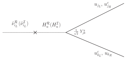
Figure 1: Feynman diagram contributing to the decay of the scalar (pseudoscalar) left sneutrino into up-type quarks, through its mixing with $H^{\mathcal{R}}_{u}$ ($H^{\mathcal{I}}_{u}$).

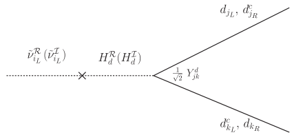
Figure 2: Feynman diagram contributing to the decay of the scalar (pseudoscalar) left sneutrino into down-type quarks, through its mixing with $H^{\mathcal{R}}_{d}$ ($H^{\mathcal{I}}_{d})$.

The scalar sneutrino $\widetilde{\nu}^{\mathcal{R}}_{iL}$ can have nevertheless a sizable mixing with $H^{\mathcal{R}}_{u}$. Although the mixing of the latter with $H^{\mathcal{R}}_{d}$ makes also the mass insertion approximation unreliable for this case shown in Fig. 1, the numerical computation using the interaction in Eq. (172) gives BR($h_{2,3}\to\bar{c}c)=0.033$ for the BP of Table 1. This can be compared with the much smaller result above of the pseudoscalar sneutrino. Because of the same reason as before, the mass insertion approximation cannot be used to estimate the interaction in Fig. 2 for the decay of the $\widetilde{\nu}^{\mathcal{R}}_{iL}$ into down-type quarks, through its mixing with $H^{\mathcal{R}}_{d}$. The numerical result of Table 1 using the interaction in Eq. (174), shows that the BR into bottom quarks is the largest one with a value BR($h_{2,3}\to\bar{b}b)=0.468$.

The mass insertion approximation can be used nevertheless for the $\widetilde{\nu}^{\mathcal{I}}_{iL}$ decay into down-type quarks shown in Fig. 2, because, in a crude approximation, one could say that $H^{\mathcal{I}}_{d}$ cannot mix with $H^{\mathcal{I}}_{u}$. Then, from Eq. (92) one can deduce that the dominant value of the coupling for the mixing between the sneutrino $\widetilde{\nu}^{\mathcal{I}}_{i}$ and the Higgs $H^{\mathcal{I}}_{d}$ is given by $\frac{1}{2}Y^{\nu}_{il}\lambda_{m}v_{lR}v_{mR}$. This is suppressed by the neutrino Yukawa coupling with respect to the squared mass of Eq. (86), thus, we can take advantage of the mass insertion technique and, their ratio determines the value of the sneutrino propagator. Armed with that, one can straightforwardly obtain the following expression for the largest effective interaction of the pseudoscalar sneutrino decay into down-type quarks:

$$\frac{Y^{b}\,Y^{\nu}}{\lambda}\frac{\lambda v_{R}}{(2A^{\lambda}+\sqrt{2}\kappa v_{R})\tan\beta}\ .$$ (44)

The complete interaction that we use for the numerical computation can be found in Eq. (175). For the BP of Table 1, we obtain BR($A_{2,3}^{0}\to\bar{b}b)=0.0017$.

Let us finally remark that for a tau sneutrino LSP of a similar mass of about 126 GeV as the electron and muon sneutrinos in Table 1, we can see in Table 2 that the results for these BRs are very similar.

Decay into photons

As a consequence of the mixing of the scalar sneutrino with $H^{\mathcal{R}}_{u,d}$ discussed above, a sizeable decay channel into photons is generated

$$\widetilde{\nu}^{\mathcal{R}}_{iL}\rightarrow\gamma\gamma\ ,$$ (45)

mainly through $W^{\pm}$ and top-quark loops, with BR($h_{2,3}\to\gamma\gamma)=0.003$ as shown in Tables 1 and 2. For an early work analyzing $\tilde{\nu}_{L}\rightarrow\gamma\gamma$ in the context of trilinear ${R}_{p}/\hskip 5.69046pt$, see Ref. BarShalom:1998xz , where a negligible BR$\sim 10^{-6}$ was obtained. This decay of the scalar sneutrino into two photons in a way not very different from the Higgs, can be very interesting for our purposes. Let us recall in this sense that the Higgs was discovered thanks to this kind of decay. Although the associated BR is far from being the dominant one, the diphoton signal is very clear and easy to disentangle from the SM backgrounds.

Notice however, that for other masses of the sneutrino as in Tables 3–5, the BR to photons is decreased. For example, in Table 3 one obtains BR($h_{2,3}\to\gamma\gamma)=0.0005$. This is because the mixing of the scalar left sneutrino with the SM Higgs is reduced when the separation between their masses is increased. In addition, the BR of the $H^{\mathcal{R}}_{u}$ to diphoton is maximal in the vicinity of the mass of the SM Higgs.

Decays into leptons

The mass insertion approximation can be used as before for the $\widetilde{\nu}^{\mathcal{I}}_{iL}$ decay into down-type quarks, but now for its decay into leptons shown in Fig. 3. Therefore, the largest effective interaction is given by Eq. (44) exchanging the bottom Yukawa coupling $Y^{b}$ by the tau Yukawa coupling $Y^{\tau}$:

$$\frac{Y^{\tau}\,Y^{\nu}}{\lambda}\frac{\lambda v_{R}}{(2A^{\lambda}+\sqrt{2}\kappa v_{R})\tan\beta}\ .$$ (46)

For the interaction shown in Fig. 4, which also contributes to the decay of the left sneutrino into leptons, the discussion is more subtle. First of all, it is necessary to proceed through a double mass insertion in the fermion propagator. Second, the Yukawa coupling in the vertex is directly related to the family of the LSP, thus for an electron or muon sneutrino, the effective interaction for the pseudoscalar (and the scalar) sneutrino decay is given respectively by

$$\frac{Y^{e,\mu}\,Y^{\nu}}{\sqrt{2}\lambda}\ ,$$ (47)

whereas for a pseudoscalar (and scalar) sneutrino of the third family one obtains

$$\frac{Y^{\tau}\,Y^{\nu}}{\sqrt{2}\lambda}\ .$$ (48)

Figure 3: Feynman diagram contributing to the decay of the scalar (pseudoscalar) left sneutrino into leptons, through its mixing with $H^{\mathcal{R}}_{d}$ ($H^{\mathcal{I}}_{d}$).

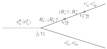
Figure 4: Feynman diagram contributing to the decay of the scalar and pseudoscalar left sneutrino into leptons, through the mixing between charged Higgsinos and leptons.

The complete interactions for the decays can be found in Appendix C. In particular, the relevant diagrams shown in Figs. 4 and 3 correspond to the first and third term, respectively, multiplying the projectors $P_{L,R}$ in Eqs. (176) and (177).

For an electron sneutrino LSP the contribution in Eq. (47) is proportional to $Y^{e}$, and therefore suppressed with respect to the one in Eq. (46), where typically $\frac{\lambda v_{R}}{(2A^{\lambda}+\sqrt{2}\kappa v_{R})\tan\beta}\approx 10^{-2}$. For a muon sneutrino LSP, however, $Y^{\mu}$ is larger than $Y^{e}$ and we obtain for the BP in Table 1 that the contribution in Eq. (47) is a factor of order 3 larger than that of Eq. (46). See e.g. in Table 1 that BR($A_{2}^{0}\to{\mu}^{\pm}\mu^{\mp})=0.0055$ whereas BR($A_{2}^{0}\to{\tau}^{\pm}\tau^{\mp})=0.0003$. Notice also that BR($A_{2}^{0}\to\bar{b}b)=0.0017$ is larger than the later mainly because of the factor 3 of color that has to be included in the computation.

On the other hand, for a tau sneutrino LSP, the contribution in Eq. (48) is larger than those in Eqs. (44) and (46). As a consequence, in this case one dominant decay channel for the pseudoscalar (and scalar) left sneutrino is the one shown in Fig. 4 into leptons

$$\widetilde{\nu}^{\mathcal{I},\mathcal{R}}_{\tau L}\rightarrow\tau^{+}_{L}l^{-}_{L}\ ,\tau^{-}_{R}l^{+}_{R}\ ,$$ (49)

where $l=e,\mu,\tau$. In Table 2, we see for example that $\sum_{l=e,\mu,\tau}BR(A^{0}_{2}\to{\tau}^{\pm}l^{\mp})=0.55$. Similar results, 0.44, 0.67, and 0.75, are obtained in Tables 3–5, respectively, where other tau sneutrino masses are analyzed.

Decays into neutrinos

The Feynman diagrams shown in Fig. 5 describe the decay of the scalar and pseudoscalar left sneutrino into neutrinos. The approximate expressions for the effective couplings can easily be deduced, as:

$$g^{\prime 2}\frac{v_{L}}{4M_{1}}\ ,\;\;\;\;g^{2}\frac{v_{L}}{4M_{2}}\ .$$ (50)

The complete interactions are given in Appendix C. The above values are a rough approximation of the first and second terms, respectively, multiplying the projectors $P_{L,R}$ in Eqs. (178) and (179).

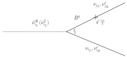
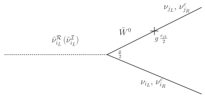
(a)	(b)

Figure 5: Feynman diagrams contributing to the decay of the scalar (pseudoscalar) left sneutrino into neutrinos, through the mixing between (a) $\tilde{B}$ and neutrinos, (b) $\tilde{W}^{0}$ and neutrinos.

For an electron or muon pseudoscalar sneutrino LSP, the contributions in Eq. (50) are of the order of 10 larger than the largest one in Eq. (47) which is proportional to $Y^{\mu}$. This is the reason why in Table 1 we obtain BR($A_{2}^{0}\to\nu\nu)=0.97$ and BR($A_{3}^{0}\to\nu\nu)=0.99$. As a consequence, the dominant decay channel is the one shown in Fig. 5 into neutrinos

$$\widetilde{\nu}^{\mathcal{I}}_{i_{L}}\rightarrow\nu_{i_{L}}\nu_{j_{L}}\ ,\nu_{i_{R}}^{c}\nu_{j_{R}}^{c}\ .$$ (51)

For a tau sneutrino LSP, the contributions in Eq. (50) are of the same order as that in Eq. (48), and therefore there are two dominant decay channels, those in Eqs. (51) and (49). The relative size between them depends on the values of the gaugino masses $M_{1}$ and $M_{2}$ necessary to reproduce the correct neutrino physics as discussed in Section 4, and the left sneutrino VEVs $v_{iL}$. In Table 2, we see for example that $\sum_{l=e,\mu,\tau}BR(A^{0}_{2}\to{\tau}^{\pm}l^{\mp})=0.55$ vs. BR($A_{2}^{0}\to\nu\nu)=0.44$.

As we will discuss in detail in the next section, scalar and pseudoscalar sneutrinos can be produced in pairs at the LHC, and as a consequence, some of the above decay modes can give rise to detectable signals. In particular, this is the case of diphoton plus missing transverse energy (MET) from sneutrinos of any family combining the channel in Eq. (45) with that of Eq. (51), and diphoton plus leptons from tau sneutrinos combining the channels in Eqs. (45) and (49). An interesting multilepton signal can also be produced combining the decay channels for scalar and pseudoscalar tau sneutrinos in Eq. (49). Although a signal with leptons plus MET is in principle possible, it suffers from a significant background and is unlikely to be observed. To have signals of diphoton plus jets or multijets is also possible, but disfavored with respect to the signals discussed here.

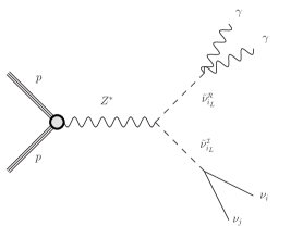
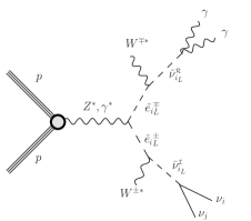
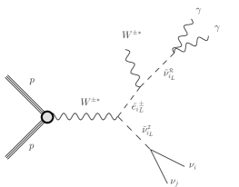
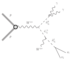
a) b) c) d)

Figure 6: Dominant decay channels into diphoton plus neutrinos from a pair production at the LHC of scalar and pseudoscalar sneutrinos LSP of any of the three families, $\widetilde{\nu}^{\mathcal{I}}_{iL}$, with $i=e,\mu,\tau$. Filled circles indicate effective interactions.

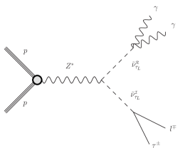
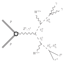
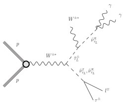
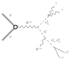
a) b) c) d)

Figure 7: Dominant decay channels into diphoton plus leptons ($l=e,\mu,\tau$) from a pair production at the LHC of scalar and pseudoscalar sneutrinos LSP of the third family $\widetilde{\nu}_{\tau L}$. Filled circles indicate effective interactions.

6 Detection at the LHC

The dominant pair production channels of sleptons at large hadron colliders were studied in Refs. Dawson:1983fw ; Eichten:1984eu ; delAguila:1990yw ; Baer:1993ew ; Baer:1997nh ; Bozzi:2004qq . In Figs. 6–8, we show the detectable signals discussed above from a pair production at the LHC of sneutrinos LSP. The sparticles are denoted in the figures by their dominant composition.

Concerning the sneutrino production, the direct one of e.g. Fig. 6a occurs via a $Z$ channel giving rise to a pair of scalar and pseudoscalar left sneutrinos. As discussed in Section 4, these states have essentially degenerate masses and therefore are co-LSPs. On the other hand, since the left slepton in the same $SU(2)$ doublet as the left sneutrino, it becomes the NLSP, and its direct production and decay is another important source of the sneutrino LSP. In particular, pair production can be obtained through a $\gamma$ or a $Z$ decaying into $\tilde{e}^{+}_{iL}\tilde{e}^{-}_{iL}$ (Fig. 6b), with the sleptons dominantly decaying into a (scalar or pseudoscalar) sneutrino plus an off-shell $W^{\pm}$ producing a soft meson or a pair of a lepton and a neutrino ($\tilde{e}^{\pm}_{iL}\to e^{\pm}_{j}\ \nu_{k}\ \widetilde{\nu}^{\mathcal{R},\mathcal{I}}_{lL}$), which are usually undetectable. Besides, sneutrinos can be pair produced through a $W^{\pm}$ decaying into $\tilde{e}^{\pm}_{iL}\widetilde{\nu}_{jL}$ (Figs. 6c-d), with the slepton decaying as before.

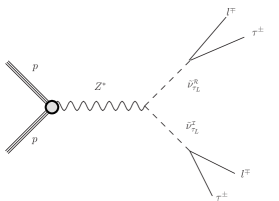
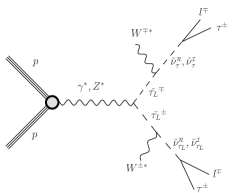
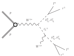
a) b) c)

Figure 8: Decay channels into multileptons ($l=e,\mu,\tau$) from a pair production at the LHC of scalar and pseudoscalar sneutrinos LSP of the third family $\widetilde{\nu}_{\tau L}$. Filled circles indicate effective interactions.

Concerning the signals, we will study first diphoton plus MET arising from the production and decay of a pair of sneutrinos $\widetilde{\nu}^{\mathcal{I}}_{i_{L}}$ $\widetilde{\nu}^{\mathcal{R}}_{i_{L}}$ of any family, $i=e,\mu,\tau$, as shown in Fig. 6. Second, we will focus on other channels that can be produced via the $\widetilde{\nu}_{\tau_{L}}$ LSP, given the large value of the tau Yukawa coupling. This is the case of diphoton plus leptons, and multileptons, as shown in Figs. 7 and 8, respectively.

These signatures for a sneutrino LSP are similar to the final states presented in several analysis of ATLAS and CMS. In particular, those including photons plus MET/leptons (see for example Refs. Aaboud2016 ; Aad:2016tuk ; Khachatryan:2017qgo ; Khachatryan:2016iqn ; Khachatryan:2016ojf ; ATLAS-CONF-2016-096 ). However, these searches are designed typically towards the production of colored sparticles in the context of $R_{p}$ conservation. Therefore, the analysis normally requires a large amount of MET, several energetic jets or a large effective mass. Thus, these searches are inefficient looking for events of direct pair production of the sneutrino in our scenario.

We have also confronted all our BPs with LHC searches Aad:2016tuk ; Aaboud:2016uro ; Aaboud:2016tnv ; Aaboud:2016zdn ; Aad:2016qqk ; Aad:2016eki ; Aaboud:2016lwz ; ATLAS-CONF-2015-082 ; ATLAS-CONF-2016-013 ; ATLAS-CONF-2016-050 ; ATLAS-CONF-2016-076 ; ATLAS-CONF-2016-096 using CheckMATE 2 Dercks:2016npn ; deFavereau:2013fsa ; Cacciari:2011ma ; Cacciari:2005hq ; Cacciari:2008gp ; Read:2002hq , and LEP searches using HiggsBounds-4.3.1 Bechtle:2008jh ; Bechtle:2011sb ; Bechtle:2013gu ; Bechtle:2013wla ; Bechtle:2015pma . In the case of the multilepton signal, there exist generic searches for production of three or more leptons, which include also signal regions with a low missing transverse momentum and total transverse energy (see Refs. Chatrchyan:2012mea ; Chatrchyan:2014aea ). In these works, by lepton is meant $e$, $\mu$ or hadronically decaying $\tau$ ($\tau_{\mathrm{h}}$) candidate. These searches are close to be sensitive to our signal, and an updated analysis with current data could put constraints on the sneutrino LSP scenario. Let us finally remark that past collider searches in the context of trilinear ${R}_{p}/\hskip 5.69046pt$ couplings Aaltonen:2010fv ; Abazov:2010km ; Achard:2001ek ; Heister:2002kq ; Heister:2002jc ; Abbiendi:2003rn ; Abdallah:2003xc ; CMS:2015neg ; Aad:2014aqa ; Khachatryan:2015dcf ; ATLAS:2015nsi ; Aad:2015pfa ; Khachatryan:2016ovq are ineffectual for our scenario.

Table 6: Madgraph cuts. $P_{T}$ is given in GeV.

$P_{T}$ for $jets$	$|\eta|$ for $jets$	$P_{T}$ for $e$, $\mu$	$|\eta|$ for $e$, $\mu$	$P_{T}$ for $\gamma$	$|\eta|$ for $\gamma$
$>20$	$<5$	$>10$	$<2.5$	$>10$	$<2.5$

Table 7: PGS configuration. ECAL and HCAL stand for Electromagnetic Calorimeter and Hadronic Calorimeter, respectively.

$\eta$ cells in calorimeter	81	$\phi$ cells in calorimeter	63
$\eta$ width of calorimeter cells	$0.1$	$\phi$ width of calorimeter cells	0.09973
ECAL resolution	0.01	ECAL resolution $\times\sqrt{E}$ (GeV1/2)	0.1
HCAL resolution $\times\sqrt{E}$ (GeV1/2)	0.8	MET resolution	0.2
Calorimeter cell edge crack fraction	0.00	Jet finding algorithm	anti-$k_{t}$ Cacciari:2008gp
Calorimeter trigger cluster	3.0	Calorimeter trigger cluster	0.5
finding seed threshold		finding shoulder threshold
Calorimeter $k_{t}$ cluster finder	0.7	Outer radius of tracker (m)	1.0
one size ($\Delta$R)
Magnetic field (T)	2.0	Sagitta resolution (m)	$5\times 10^{-6}$
Track finding efficiency	0.98	Minimum track $P_{T}$ (GeV/c)	0.30
Tracking $\eta$ coverage	2.5	e/gamma $\eta$ coverage	3.0
Muon $\eta$ coverage	2.4	Tau $\eta$ coverage	2.0

The strategy that we will follow for the analyses of the sneutrino signals in the $\mu\nu{\rm SSM}$ is the following. Ten thousand events are generated for each case with MadGraph5_aMC@NLO Alwall:2014hca at leading order (LO) of perturbative QCD simulating the production of the described process. We include the next-to-leading order (NLO) Baer:1997nh and next-to-leading logarithmic accuracy (NLL)  Fuks:2013lya results using a $K$-factor of about 1.2. The hard process simulation is then passed for decay and hadronization to PYTHIA Sjostrand:2006za . The output is passed through a naive and fast detector simulation (PGS) pgs . The standard card for MadGraph5_aMC@NLO is used, which includes the cuts presented in Table 6. PYTHIA is executed with initial state radiation (ISR), final state radiation (FSR) and multiple interactions switched on. Besides, PYTHIA will consider the $\tau$ lepton as stable to make it decay with the TAUOLA Jadach:1990mz ; Jadach:1993hs routine within PGS. The package PGS is finally executed using a card designed for ATLAS, as shown in Table 7. The output of PGS is passed through some selection criteria to avoid overlapping and to discard the events outside the detector coverage according to Ref. Aad:2014iza . That is, first candidate events should pass the requirements of Table 8. After the previous process, overlapping objects are removed applying the following requirements in this precise order: First, if two electrons as candidates are identified within $\Delta R=0.05$ of each other, the one with lower transverse momentum ($P_{T}$) is discarded. Here $\Delta R$ is defined as $\sqrt{(\Delta\Phi)^{2}+(\Delta\eta)^{2}}$, where $\Delta\Phi$ is the difference in involved azimuthal angles while $\Delta\eta$ is the difference of concerned pseudo-rapidities. Then if an electron and a jet candidates are within $\Delta R=0.2$ of each other, the jet is discarded. All remaining leptons are required to be separated by more than $\Delta R=0.4$ from the closest remaining jet. Whenever an electron and a muon candidates overlap within $\Delta R=0.01$, both are discarded. Also, if two muons are separated by less than $\Delta R=0.05$, both are removed. $\tau$’s as candidates are required to be separated by more than $\Delta R=0.2$ from the closest $e$ or $\mu$; otherwise they are discarded. Finally, photons are required to be separated by $\Delta R=0.4$ from any reconstructed jet and $\Delta R=0.01$ from any $e$ Aad:2015hea . A similar process, with a higher number of events when required by precision, is implemented to generate background samples at NLO.

Table 8: Event filtering. $P_{T}$ is given in GeV.

$P_{T}$	$|\eta|$	$P_{T}$	$|\eta|$	$P_{T}$	$|\eta|$	$P_{T}$	$|\eta|$	$P_{T}$	$|\eta|$
for $jets$	for $jets$	for $e$	for $e$	for $\mu$	for $\mu$	for $\tau_{\mathrm{h}}$	for $\tau_{\mathrm{h}}$	for $\gamma$	for $\gamma$
$>30$	$<4.5$	$>15$	$<2.47$	$>10$	$<2.5$	$>10$	$<2.5$	$>25$	$2.37$
			& outside						& outside
			$1.37-1.52$						$1.37-1.52$

Diphoton plus MET

The pair production of left sneutrinos can generate one scalar and one pseudoscalar, as shown in Fig. 6. This opens the possibility of the pseudoscalar sneutrino decaying into neutrinos, i.e., producing MET, and the scalar sneutrino decaying into two photons in a way not very different from the Higgs.

Table 9: Analysis of the signal with diphoton plus MET from production and decay of a pair of sneutrino co-LSPs of the type $\widetilde{\nu}_{eL}$ or $\widetilde{\nu}_{\mu L}$, corresponding to the BP in Table 1. Production cross sections are shown in fb in the first box for a $\widetilde{\nu}_{eL}/\widetilde{\nu}_{\mu L}$ mass of 125.4 GeV. The number of events of the signal and background is shown in the second box, together with the effect of a set of cuts, assuming 13 TeV center-of-mass energy with $\mathcal{L}=300$ fb^-1. Energies, momenta and invariant mass are given in GeV.

$\sigma(pp\to Z^{*}\to h_{2}A^{0}_{2})$	$107.08$
$\sigma(pp\to\gamma^{*},Z^{*}\to H_{2}^{+}H_{2}^{-}\to h_{2}A_{2}^{0}+W^{+}_{\text{soft}}W^{-}_{\text{soft}})$	$21.89$
$\sigma(pp\to W^{\pm^{*}}\to H_{2}^{\pm}\ h_{2}/A_{2}^{0}\to h_{2}A_{2}^{0}+W^{\pm}_{\text{soft}})$	$142.8$
$\sigma(pp\to Z^{*}\to h_{3}A^{0}_{3})$	$106.536$
$\sigma(pp\to\gamma^{*},Z^{*}\to H_{3}^{+}H_{3}^{-}\to h_{3}A_{3}^{0}+W^{+}_{\text{soft}}W^{-}_{\text{soft}})$	$20.12$
$\sigma(pp\to W^{\pm^{*}}\to H_{3}^{\pm}\ h_{3}/A_{3}^{0}\to h_{3}A_{3}^{0}+W^{\pm}_{\text{soft}})$	142.4

Dataset	$\mathrm{N_{ev}}$	${E}_{T}^{\mathrm{miss}}$	$P_{T1}^{\gamma_{1}}$	$P_{T2}^{\gamma_{2}}$	$N_{\gamma}$=2	$N_{l}=0$	$\Delta R$	$M_{\gamma\gamma}\in$
		$>200$	$>100$	$>50$			$<1.5$	$[115,135]$
Signal	449.45$\pm 0.02$	103.6$\pm 0.8$	80.3$\pm 0.7$	41.0$\pm 0.5$	41.0$\pm 0.5$	36.4$\pm 0.5$	35.9$\pm 0.5$	34.1$\pm 0.5$
2$jets$	$10^{7}$	0	0	0	0	0	0	0
+I/FSR
$jet$	$10^{7}$	0	0	0	0	0	0	0
+I/FSR
H (ggF)	5424	0	0	0	0	0	0	0
$Z$+H	120.8$\pm$0.4	6.9$\pm$0.3	5.9$\pm$0.3	3.3$\pm$0.2	3.3$\pm$0.2	3.2$\pm$0.2	3.1$\pm$0.2	2.9$\pm$0.2
$Z$+ISR	11310$\pm$40	104$\pm$11	97$\pm$10	33$\pm$6	33$\pm$6	33$\pm$6	8$\pm$3	$1\pm$1
$W$+FSR	$2.14\times 10^{5}$	60$\pm$9	57$\pm$9	13$\pm$4	13$\pm$4	6$\pm$3	1.4$\pm$1.4	0
	$\pm 76$
$\frac{S}{\sqrt{B}}$	—	7.9$\pm$0.5	6.3$\pm$0.4	5.9$\pm$0.7	5.9$\pm$0.7	5.6$\pm$0.7	10$\pm$2	17$\pm 3$

In what follows, we will discuss first the case of sneutrinos co-LSPs of the first two families ($\widetilde{\nu}_{eL}$, $\widetilde{\nu}_{\mu L}$) with masses of about 125 GeV as representative in order to search for a signal. This is because the sensible range of masses turns out to be

$$118\lesssim m_{\widetilde{\nu}_{iL}}\lesssim 132\ \,\textrm{GeV}\ ,$$ (52)

in order to treat the sneutrinos as promptly decaying particles with a decay length $\;<$$\sim\;$ 0.1 mm. For the case of the tau sneutrino, $\widetilde{\nu}_{\tau_{L}}$, where decay lengths of this order can be obtained for masses $\;>$$\sim\;$ 95 GeV, the above mass range is still valid because outside it the number of events turns out to be too small, as we will discuss below.

The case of $\widetilde{\nu}_{e_{L}}$ and $\widetilde{\nu}_{\mu_{L}}$ co-LSPs is shown in Table 9. The cross sections for the pair production of sneutrinos calculated by MadGraph5_aMC@NLO 2.3.2.2 at LO for 13 TeV center-of-mass energy, including a $K$-factor of 1.2 for the NLO results, are shown in the first box of that Table. The first, second and third rows of that box correspond to the diagrams in Figs. 6a, 6b and 6c-d, respectively. Taking into account these values for the cross sections, the BRs of the corresponding Table 1, and using an integrated luminosity of $\mathcal{L}=300$ fb^-1, we obtain a signal with about 449 events. Although this BP suffers from a significant SM background mainly due to the Z+$H$ channel which decays in a similar way, we found that the number of expected events for the signal is still sufficient to give a significant evidence. The effect of a set of cuts on missing transverse energy ${E}_{T}^{\mathrm{miss}}$, $P_{T}$ for the leading and sub-leading photons, a lepton veto, a maximum angular separation of photons, and a selection cut on the invariant mass of the diphoton system, is summarized in the second box of Table 9. As a final result of the analysis, we obtain 34.1 $\pm 0.5$ events with a significant evidence of $\frac{S}{\sqrt{B}}=17\pm 3$. For $\mathcal{L}=100$ fb^-1 to be reached in Run 2 we just have to rescale the number of events by a factor $1/3$ and correspondingly the significance by $1/\sqrt{3}$. For completeness, we show in Table 10 the results for this BP with 14 TeV center-of-mass energy.

Table 10: The same as in Table 9 but showing the production cross sections and the event sample generated with 14 TeV center-of-mass energy.

$\sigma(pp\to Z^{*}\to h_{2}A^{0}_{2})$	$119.95$
$\sigma(pp\to\gamma^{*},Z^{*}\to H_{2}^{+}H_{2}^{-}\to h_{2}A_{2}^{0}+W^{+}_{\text{soft}}W^{-}_{\text{soft}})$	$25.43$
$\sigma(pp\to W^{\pm^{*}}\to H_{2}^{\pm}\ h_{2}/A_{2}^{0}\to h_{2}A_{2}^{0}+W^{\pm}_{\text{soft}})$	$160.7$
$\sigma(pp\to Z^{*}\to h_{3}A^{0}_{3})$	$119.83$
$\sigma(pp\to\gamma^{*},Z^{*}\to H_{3}^{+}H_{3}^{-}\to h_{3}A_{3}^{0}+W^{+}_{\text{soft}}W^{-}_{\text{soft}})$	$23.35$
$\sigma(pp\to W^{\pm^{*}}\to H_{3}^{\pm}\ h_{3}/A_{3}^{0}\to h_{3}A_{3}^{0}+W^{\pm}_{\text{soft}})$	158.9

Dataset	$\mathrm{N_{ev}}$	${E}_{T}^{\mathrm{miss}}$	$P_{T1}^{\gamma_{1}}$	$P_{T2}^{\gamma_{2}}$	$N_{\gamma}$=2	$N_{l}=0$	$\Delta R$	$M_{\gamma\gamma}\in$
		$>200$	$>100$	$>50$			$<1.5$	$[115,135]$
Signal	503.40$\pm$0.02	116.3$\pm$0.9	95.0$\pm$0.8	50.8$\pm$0.6	50.5$\pm$0.6	43.8$\pm$0.6	43.3$\pm$0.6	38.8$\pm$0.6
2$jets$	$10^{7}$	0	0	0	0	0	0	0
+I/FSR
$jet$	$10^{7}$	0	0	0	0	0	0	0
+I/FSR
H (ggF)	6104	0	0	0	0	0	0	0
$Z$+H	133.76	7.9$\pm$0.3	6.7$\pm$0.3	3.5$\pm$0.2	3.5$\pm$0.2	3.4$\pm$0.2	3.3$\pm$0.2	3.0$\pm$0.2
	$\pm 0.01$
$Z$+ISR	9284.91	90$\pm$3	82$\pm$3	26$\pm$2	26$\pm$2	25$\pm$2	8$\pm$1	$1.2\pm$0.3
	$\pm 0.09$
$W$+FSR	23708$\pm 2$	57$\pm$9	54$\pm$9	5$\pm$3	5$\pm$3	1.6$\pm 1.61$	0	0
$\frac{S}{\sqrt{B}}$	—	9.3$\pm$0.5	8.0$\pm$0.4	8.7$\pm$0.7	8.7$\pm$0.7	8.1$\pm$0.6	13.0$\pm$0.8	19$\pm 1$

Concerning the case of the $\widetilde{\nu}_{\tau_{L}}$ LSP of a similar mass, we can see in the fourth box of Table 2 that it has a significant BR to neutrinos. After a straightforward computation, we obtain a number of events of $7.5\pm 0.2$. The background is the same as in Table 9, and therefore we obtain $\frac{S}{\sqrt{B}}\sim 3.8\pm 0.6$. This BP can also give rise to a signal with diphoton plus leptons, to be analyzed subsequently, implying that a tau left sneutrino LSP could be distinguished from electron and muon left sneutrinos co-LSPs. For the other $\widetilde{\nu}_{\tau L}$ masses studied in Tables 3 and 4, although the BRs to neutrinos are still significant, the number of events of the signal diphoton plus MET turns out to be too small to be detected.

The case with all sneutrinos degenerate in mass would give rise to a superposition of the signals discussed so far. For instance, if the three families of sneutrinos have a mass of 126 GeV, the number of events expected for the signal diphoton plus MET will be the sum of both contributions discussed above, that is $41.6\pm 0.5$ events with a significance of $\frac{S}{\sqrt{B}}=21\pm 1$. In addition, the signal with diphoton plus leptons, specific for the $\widetilde{\nu}_{\tau L}$, would also be present.

Diphoton plus leptons

For the case of the left sneutrino LSP dominated by the tau composition, $\widetilde{\nu}_{\tau L}$, another expected signal is diphoton plus leptons, as shown in Fig 7. For this signal the adequate range of masses turns out ot be

$$95\lesssim m_{\widetilde{\nu}_{\tau_{L}}}\lesssim 145\ \,\textrm{GeV}\ .$$ (53)

For the lower bound, notice that the selection cuts used to discriminate the decay of the sneutrino from the background require energetic photons and a large amount of missing energy. Therefore, a sneutrino with a small mass would lead to a small boost of the final photons and neutrinos. Thus reducing the mass of the sneutrino reduces the number of events in the signal region, although the cross section increases. Moreover, when the separation between the masses of the scalar left sneutrino and the SM Higgs is increased, the BR to diphoton is decreased. Altogether, the number of events drops fast when the mass of the left sneutrino is below 95 GeV. Actually, we already mentioned that about this mass is also the limit where the LSP cannot be treated as a promptly decaying particle. On the other hand, the decrease of the cross section for large sneutrino masses, and therefore of the number of events, gives rise to the upper bound of 145 GeV.

Table 11: Analysis of the signal with two photons plus leptons from production and decay of a pair of $\widetilde{\nu}_{\tau L}$ LSPs, corresponding to the BP in Table 2. Production cross sections are shown in fb in the first box for a $\widetilde{\nu}_{\tau L}$ mass of 126.4 GeV. The number of events of the signal and background is shown in the second box, together with the effect of a set of cuts, assuming 13 TeV of energy with $\mathcal{L}=300$ fb^-1. Momenta and invariant mass are given in GeV.

$\sigma(pp\to Z^{*}\to h_{2}A^{0}_{2})$	103.58
$\sigma(pp\to\gamma^{*},Z^{*}\to H_{2}^{+}H_{2}^{-}\to h_{2}A^{0}_{2}\ +W^{+}_{\text{soft}}W^{-}_{\text{soft}})$	21.91
$\sigma(pp\to W^{\pm^{*}}\to H_{2}^{\pm}h_{2}/A^{0}_{2}\to h_{2}A^{0}_{2}\ +W^{\pm}_{\text{soft}})$	$138.36$
$\sigma(pp\to W^{\pm^{*}}\to H_{2}^{\pm}h_{2}\to h_{2}h_{2}\ +W^{\pm}_{\text{soft}})$	$69.18$

Dataset	$\mathrm{N_{ev}}$	$P_{T1}^{\gamma_{1}}$	$P_{T2}^{\gamma_{2}}$	$N_{\gamma}$=2	$N_{\tau_{had}}=1\,\&$	$\Delta R<1.5$	$M_{\gamma\gamma}\in$
		$>100$	$>50$		$N_{e,\mu,\tau_{had}}>1$		$[115,135]$
Signal	128.136$\pm$0.007	67.8$\pm$0.4	25.4$\pm 0.3$	25.4$\pm$0.3	5.9$\pm$0.2	4.9$\pm 0.1$	4.7$\pm$0.1
$Z$+H	73.26$\pm$0.06	35.4$\pm$0.3	10.0$\pm$0.3	10.0$\pm$0.3	0.54$\pm$0.06	0.21$\pm$0.04	0.21$\pm$0.04
$W$+H	151.2$\pm$0.5	71.3$\pm$0.3	19.9$\pm$0.1	19.9$\pm$0.1	0.28$\pm$0.03	0.14$\pm$0.01	0.13$\pm$0.01
$Z$+ISR	53949$\pm$40	1394$\pm$42	210$\pm$17	210$\pm$17	7$\pm$3	0	0
$W$+FSR	71414$\pm$204	8776$\pm$116	1922$\pm$58	1922$\pm$58	17$\pm$5	0$\pm$0	$0\pm$0
$\frac{S}{\sqrt{B}}$	—	0.67$\pm$0.01	$0.55\pm 0.02$	0.55$\pm$0.02	1.2$\pm$0.2	8.4$\pm$0.9	8.1$\pm 0.9$

Table 12: The same as in Table 11 but for the BP in Table 3 corresponding to a $\widetilde{\nu}_{\tau L}$ LSP with a mass of 97.8 GeV.

$\sigma(pp\to Z^{*}\to h_{1}A^{0}_{2})$	265.92
$\sigma(pp\to\gamma^{*},Z^{*}\to H_{2}^{+}H_{2}^{-}\to h_{1}A^{0}_{2}\ +W^{+}_{\text{soft}}W^{-}_{\text{soft}})$	42.67
$\sigma(pp\to W^{\pm^{*}}\to h_{1}^{\pm}h_{1}/A^{0}_{2}\to h_{1}A^{0}_{2}\ +W^{\pm}_{\text{soft}})$	$325.2$
$\sigma(pp\to W^{\pm^{*}}\to h_{1}^{\pm}h_{1}\to h_{1}h_{1}\ +W^{\pm}_{\text{soft}})$	$162.6$

Dataset	$\mathrm{N_{ev}}$	$P_{T1}^{\gamma_{1}}$	$P_{T2}^{\gamma_{2}}$	$N_{\gamma}$=2	$N_{\tau_{had}}=1\,\&$	$\Delta R$	$M_{\gamma\gamma}\in$
		$>100$	$>50$		$N_{e,\mu,\tau_{had}}>1$	$<1.5$	$[85,105]$
Signal	44.438$\pm$0.002	14.4$\pm$0.1	3.96$\pm 0.06$	3.96$\pm$0.06	0.82$\pm$0.03	0.81$\pm 0.03$	0.78$\pm$0.03
$Z$+H	73.26$\pm$0.06	35.4$\pm$0.3	10.0$\pm$0.3	10.0$\pm$0.3	0.54$\pm$0.06	0.21$\pm$0.04	0.03$\pm$0.01
$W$+H	151.2$\pm$0.5	71.28$\pm$0.3	19.9$\pm$0.1	19.9$\pm$0.1	0.28$\pm$0.03	0.14$\pm$0.01	0$\pm$0
$Z$+ISR	53949$\pm$40	1394$\pm$42	210$\pm$17	210$\pm$17	7$\pm$3	0	0
$W$+FSR	71415$\pm$204	8776$\pm$116	1922$\pm$58	1922$\pm$58	17$\pm$5	0$\pm$0	$0\pm$0
${S}/{\sqrt{B}}$	—	0.14	$0.085$	0.0085	0.17$\pm$0.03	1.4$\pm$0.2	5$\pm 1$
		$\pm 0.002$	$\pm 0.003$	$\pm 0.003$

Table 13: The same as in Table 11 but for the BP in Table 4 corresponding to a $\widetilde{\nu}_{\tau L}$ LSP with a mass of 146 GeV.

$\sigma(pp\to Z^{*}\to h_{2}A^{0}_{2})$	60.48
$\sigma(pp\to\gamma^{*},Z^{*}\to H_{2}^{+}H_{2}^{-}\to h_{2}A^{0}_{2}\ +W^{+}_{\text{soft}}W^{-}_{\text{soft}})$	14.69
$\sigma(pp\to W^{\pm^{*}}\to H_{2}^{\pm}h_{2}/A^{0}_{2}\to h_{2}A^{0}_{2}\ +W^{\pm}_{\text{soft}})$	$87.24$
$\sigma(pp\to W^{\pm^{*}}\to H_{2}^{\pm}h_{2}\to h_{2}h_{2}\ +W^{\pm}_{\text{soft}})$	$43.62$

Dataset	$\mathrm{N_{ev}}$	$P_{T1}^{\gamma_{1}}$	$P_{T2}^{\gamma_{2}}$	$N_{\gamma}$=2	$N_{\tau_{had}}=1\,\&$	$\Delta R$	$M_{\gamma\gamma}\in$
		$>100$	$>50$		$N_{e,\mu,\tau_{had}}>1$	$<1.5$	$[135,155]$
Signal	24.47$\pm$0.01	15.51$\pm$0.06	6.72$\pm 0.06$	6.72$\pm$0.06	1.68$\pm$0.03	1.09$\pm 0.03$	1.01$\pm$0.03
$Z$+H	73.26$\pm$0.06	35.4$\pm$0.3	10.0$\pm$0.3	10.0$\pm$0.3	0.54$\pm$0.06	0.21$\pm$0.04	0.03$\pm$0.01
$W$+H	151.2$\pm$0.5	71.3$\pm$0.3	19.9$\pm$0.1	19.9$\pm$0.1	0.28$\pm$0.03	0.14$\pm$0.01	0$\pm$0
$Z$+ISR	53949$\pm$40	1394$\pm$42	210$\pm$17	210$\pm$17	7$\pm$3	0	0
$W$+FSR	71414$\pm$204	8776$\pm$116	1922$\pm$58	1922$\pm$58	17$\pm$5	0$\pm$0	$0\pm$0
${S}/{\sqrt{B}}$	—	0.153	$0.145$	0.145	0.34$\pm$0.06	1.8$\pm$0.2	6$\pm 2$
		$\pm 0.002$	$\pm 0.004$	$\pm 0.004$

The results for a sneutrino mass of about 126 GeV, similar to the one studied above, are shown in Table 11. The discussion is similar to that above, although in this case we do not have two families of sneutrinos with degenerate masses, and therefore the different production mechanisms will only give rise to $\widetilde{\nu}_{{\tau}}\widetilde{\nu}_{{\tau}}$, thus reducing the number of events. These are further suppressed by the BR($A^{0}_{2}\to{\tau}^{\pm}l^{\mp}$) compared to BR($A^{0}_{2}\to\nu\nu$) in the case of $\widetilde{\nu}_{e,\mu}$ LSP. Nevertheless, this signal with photons plus leptons is very attractive and worth to be searched at the LHC.

Now, a different set of cuts is taken into account for convenience, as shown in the second box of Table 11. To distinguish the signal from the background in this case, instead of using the missing energy coming from neutrinos, we require two leptons in the final state of which one of them must be an hadronically decaying tau. Since every leptonic decay of the tau sneutrino includes at least one tau, we expect to reduce significantly more the background than the signal itself. Using an integrated luminosity of $\mathcal{L}=300$ fb^-1, we obtain $4.7\pm 0.1$ events with a significant evidence of $\frac{S}{\sqrt{B}}=8.1\pm 0.9$.

In order to confirm the range of sneutrino masses of about 95–145 GeV adequate to observe this kind of signal, we have also analyzed in Tables 12 and 13 the two extreme cases of about 98 and 146 GeV, respectively. Note that for both cases the BR of the scalar sneutrino decaying into photons is supressed with respect to the previous case of 126 GeV. Although for the case of 98 GeV, the cross sections are increased with respect to the case of 126 GeV in Table 11, the final products would have less $P_{T}$, and $E_{T}$, thus the efficiency of the selection cuts would be smaller. We apply the same set of selection cuts to the signal calculated with this new point as in the previous case, but selecting now a new invariant mass window for the diphoton sistem of $\pm 10$ around 98 GeV. The rest of the analysis is completely analogous, and the results are presented in the second box of Table 12. For this extreme case we still obtain 0.78 $\pm$ 0.03 events with a significant evidence of $\frac{S}{\sqrt{B}}=5\pm 1$.

Finally, to explore the largest possible value of the sneutrino mass, we have considered the case of 146 GeV. We show the final results in Table 13. As can be seen, the production cross sections are reduced with the increase of the mass. We are not considering points with sneutrino masses larger than $146\,\textrm{GeV}$ because the possible signal gets likely lost behind the SM backgrounds. The results of the different selection cuts for this extreme case are presented in the second box of Table 13. As a final result, 1.01 $\pm$ 0.03 events with a significant evidence of $\frac{S}{\sqrt{B}}=6\pm 2$ are obtained.

Table 14: Analysis of the signal with multileptons from production and decay of a pair of $\widetilde{\nu}_{\tau L}$ LSPs. The number of events of the signal and background is shown, together with the effect of a set of cuts, assuming 13 TeV center-of-mass energy with $\mathcal{L}=20$ fb^-1. The subindex $l$ in the dataset denotes leptonically decaying tops and gauge bosons. Three possible masses of $\widetilde{\nu}_{\tau L}$, 132, 146 and 311 GeV are analyzed, with the last two obtained using the BPs of Tables 4 and 5.

Dataset	$N_{l}\geq 4\ \&\ N_{\tau_{h}}\geq 2$	$N_{b}=0$	THT$\leq 20$ GeV	W-veto	Z-veto	$\frac{S}{\sqrt{B}}$
${\bar{t}t}_{l}$	$306\pm 66$	$174\pm 50$	14$\pm 14$	$0\pm 0$	$0\pm 0$	–
${\bar{t}th}$	$3\pm 2$	0$\pm 0$	$0\pm 0$	$0\pm 0$	$0\pm 0$	–
${\bar{t}t\bar{t}t}$	$0.8\pm 0.5$	$0\pm 0$	$0\pm 0$	$0\pm 0$	$0\pm 0$	–
${\bar{t}tV}_{l}$	$1.2\pm 0.3$	$0.6\pm 0.2$	$0.12\pm 0.09$	$0.12\pm 0.09$	$0.12\pm 0.09$	–
${VV}_{l}$	$6\pm 4$	$6\pm 4$	$3\pm 3$	$3\pm 3$	$3\pm 3$	–
$VVV$	$2\pm 1$	$0.8\pm 0.8$	$0\pm 0$	$0\pm 0$	$0\pm 0$	–
${tV}_{l}$	$15\pm 5$	$14\pm 5$	$8\pm 4$	$8\pm 4$	$8\pm 4$	–
${tVV}_{l}$	$1.0\pm 0.3$	$0.6\pm 0.2$	$0.10\pm 0.08$	$0.10\pm 0.08$	$0.10\pm 0.08$	–
Total	$334\pm 66$	$196\pm 64$	$25\pm 15$	$11\pm 5$	$11\pm 5$	–
Signal 132 GeV	$36\pm 2$	$36\pm 2$	$20\pm 2$	$17\pm 1$	$16\pm 1$	$4.8\pm 2.2$
Signal 146 GeV	$68\pm 3$	$66\pm 3$	$37\pm 2$	$31\pm 2$	$29\pm 2$	$8.8\pm 4.0$
Signal 311 GeV	$18.2\pm 0.5$	$17.9\pm 0.5$	$8.9\pm 0.4$	$7.6\pm 0.4$	$7.5\pm 0.2$	$2.2\pm 1.0$

Multileptons

For the tau left sneutrino, we can see in Tables 4 and 5 that the BRs for the decay of the scalar state $\widetilde{\nu}^{\mathcal{R}}_{\tau_{L}}$ into leptons are significant. This gives rise to a non negligible number of events with both sneutrinos decaying into leptons, as shown in Fig 8. With the appropriate analysis, these events could constitute a possible signal to be detected at the LHC. Moreover, these decay channels of the LSP include always at least one $\tau$, a feature that can be exploited to unravel the signal.

The main backgrounds for this type of signature would be the production of top quarks through the channels $\bar{t}t$ and $\bar{t}t\bar{t}t$; the production of gauge bosons ZZ, WW and ZW; the associated production of both $\bar{t}tV$, $tV$ and $tVV$; and the top associated Higgs production $\bar{t}th$. Since the proposed hard process would not produce quarks, we expect a hadronic activity in the events significantly smaller than the one associated with background events including a leptonically decaying top $t_{l}$. We will show that it is possible to separate the multilepton signal from the SM backgrounds. This is particularly true for sneutrinos with large masses, since the produced leptons are then expected to be more energetic than the ones produced in the decay of gauge bosons.

The Monte Carlo events generated and processed as in the previous signals, but in this case with an integrated luminosity of $\mathcal{L}=20$ fb^-1, are analyzed and summarized in Table 14 for three different sneutrino masses of 132, 146 and 311 GeV. Production cross sections for the case of 146 GeV are already shown in Table 13. For 310 GeV these are much lower. At first we select events with at least 4 leptons with $P_{T}$ $\geq$ 100, 80, 40 and 40 GeV, respectively, requiring also at least two of them to be $\tau_{\mathrm{h}}$’s. The second selection rejects events with $b$-tagged jets in order to reduce backgrounds coming from top decays. In the next step we reject events with a total transverse hadronic energy (THT) greater than 20 GeV. Finally we apply a veto to the transverse mass and invariant mass of the light leptons, compatible with the mass of the W and Z respectively. Summarizing the results shown in Table 14, it is possible to detect $\widetilde{\nu}_{\tau_{L}}$ in the mass range

$$130\lesssim m_{\widetilde{\nu}_{\tau L}}\lesssim 310\ \,\textrm{GeV}\ ,$$ (54)

decaying leptonically with a significance $\frac{S}{\sqrt{B}}$ greater than 3.

Equations (52), (53) and (54) establish the adequate range of left sneutrino masses for our analysis of the BPs introduced in Section 4, and Tables 1–5. As we can see, the masses overlap in some ranges, and in these cases the corresponding BP can give rise to different detectable signals.

7 Conclusions and outlook

We have carried out an analysis of the LHC phenomenology associated to the left sneutrino LSP in the $\mu\nu{\rm SSM}$. We have studied the dominant pair production channels, prompt decays, and the detection of the new signals.

As a result of the different behaviors of scalar and pseudoscalar sneutrino states, a diphoton signal in combination with neutrinos (producing missing transverse energy), or a diphoton with leptons, can appear at the LHC. The former can be detected with a center-of-mass energy of 13 TeV and the integrated luminosity of 100 fb^-1, for a sneutrino LSP of any family in the mass range 118–132 GeV. The diphoton plus leptons signal can be probed for the case of a tau sneutrino LSP with a mass in the range 95–145 GeV. We have discussed several benchmark points producing these signals, which undoubtedly deserve proper experimental attention. We have also shown that the number of expected events are capable of giving a significant evidence.

A multilepton signal from a tau sneutrino LSP can also appear detectable at the LHC with a center-of-mass energy of 13 TeV, even with the integrated luminosity of 20 fb^-1. It is possible to detect it in the mass range of 130–310 GeV. We have discussed that existing generic searches at the LHC are close to be sensitive to this lepton signal, suggesting that they deserve experimental attention. An updated analysis with current data could constrain the sneutrino LSP scenario.

Displaced vertices of the order of the millimeter can appear for sneutrino masses $\raise 1.29167pt\hbox{$\;<$\kern-7.5pt\raise-4.73611pt\hbox{$\sim\;$}}100$ GeV. Imposing in addition that the sneutrino mass is larger than 45 GeV, not to disturb the experimentally well measured decay width of the $Z$, we have found that the number of events can be large. For example, more than 1000 multilepton events at the parton level from the production and decay of a tau sneutrino pair can emerge for an integrated luminosity of 20 fb^-1 and 13 TeV center-of-mass energy. These events have the clear advantage that the SM backgrounds are negligible and hence the signal significance is high. However, the analysis of displaced vertices turns out to be quite complicated, and dedicated studies are necessary. The efficiency identifying events characterized by the presence of a displaced vertex has a nontrivial dependence on the position of the vertex, as well as the number of tracks and the mass associated to them, among others. Therefore, a reliable analysis requires a precise simulation of the decay length, the boost of the long-lived particle, and the particles produced in the secondary vertex. This analysis, in our model, is expected to depend on the parameters correlated with neutrino physics and is clearly beyond the scope of the present work, although we plan to cover it in a forthcoming publication prepa .

Appendix A The Superpotential and Soft Terms

We review in this Appendix the superpotential of the model and the associated soft terms, following the works of Refs. LopezFogliani:2005yw ; Escudero:2008jg ; Lopez-Fogliani:2017qzj .

Given the gauge symmetry group of the SM, $SU(3)_{C}\times SU(2)_{L}\times U(1)_{Y}$, with subscripts $C$, $L$ and $Y$ referring to color, left chirality and weak hypercharge, respectively, the superpotential of the $\mu\nu{\rm SSM}$ can be written as Lopez-Fogliani:2017qzj

$$W= \epsilon_{ab}\left(Y^{e}_{IJk}\,\hat{L}_{I}^{a}\,\hat{L}_{J}^{b}\,\hat{e}_{k}^{c}+Y^{d}_{Ijk}\,\delta_{\alpha\beta}\,\hat{L}_{I}^{a}\,\hat{Q}_{j\alpha}^{b}\,\hat{d}_{k\beta}^{c}+Y^{u}_{ij}\,\delta_{\alpha\beta}\,\hat{L}^{{}^{cb}}_{4}\,\hat{Q}_{i\alpha}^{a}\,\hat{u}_{j\beta}^{c}\right)$$ (55)

$$+ \epsilon_{ab}\,Y^{\nu}_{Ij}\,\hat{L}^{{}^{cb}}_{4}\,\hat{L}_{I}^{a}\,\hat{\nu}^{c}_{j}+\frac{1}{3}\kappa_{ijk}\,\hat{\nu}^{c}_{i}\,\hat{\nu}^{c}_{j}\,\hat{\nu}^{c}_{k}\ ,$$

where the summation convention is implied on repeated indexes, with $\alpha,\beta=1,2,3$ $SU(3)_{C}$ indexes, $a,b=1,2$ $SU(2)_{L}$ indexes with $\epsilon_{ab}$ the totally antisymmetric tensor $\epsilon_{12}=1$, and $I=i,4$ ($J=j,4$) with $i,j,k=1,2,3$ the usual family indexes of the SM and with the vector-like Higgs doublet superfields interpreted as a fourth family of vector-like lepton superfields $\hat{L}_{4}=(\hat{\nu}_{4},\hat{e}_{4})=(\hat{H}_{d}^{0},\hat{H}_{d}^{-})=\hat{H}_{d}$ and $\hat{L}_{4}^{c}=(\hat{e}^{c}_{4},\hat{\nu}^{c}_{4})=(\hat{H}_{u}^{+},\hat{H}_{u}^{0})=\hat{H}_{u}$. This interpretation is possible in the $\mu\nu{\rm SSM}$ because right-handed neutrinos are present producing the violation of $R_{p}$, and as a consequence all fields in the spectrum with the same color, electric charge and spin mix together. In particular, Higgses mix with sleptons and Higgsinos with leptons. From the theoretical viewpoint, this seems to be more satisfactory than the situation in usual SUSY models, where the Higgses are ‘disconnected’ from the rest of the matter and do not have a three-fold replication. As pointed out in Ref. Lopez-Fogliani:2017qzj , in this SUSY framework the first scalar particle discovered at the LHC is mainly a sneutrino belonging to a fourth-family vector-like doublet representation.

In order to make contact with the usual (three-family) notation of the $\mu\nu{\rm SSM}$ LopezFogliani:2005yw ; Escudero:2008jg , we can decompose the terms given by the couplings $Y^{e}_{IJk}$, $Y^{d}_{Ijk}$ and $Y^{\nu}_{Ij}$ in two type of terms: Yukawa couplings generating fermion masses, and lepton-number violating couplings. This is possible because, as discussed above, the superfields $L_{i}$ and $H_{d}$ have the same gauge quantum numbers, and therefore $\hat{L}_{I}=\hat{L}_{i},\hat{H}_{d}$. Thus, we can write superpotential (55) as follows LopezFogliani:2005yw ; Escudero:2008jg :

$$W= \epsilon_{ab}\left(Y^{e}_{ij}\,\hat{H}_{d}^{a}\,\hat{L}^{b}_{i}\,\hat{e}_{j}^{c}+Y^{d}_{ij}\,\delta_{\alpha\beta}\,\hat{H}_{d}^{a}\,\hat{Q}^{b}_{i\alpha}\,\hat{d}_{j\beta}^{c}+Y^{u}_{ij}\,\delta_{\alpha\beta}\,\hat{H}_{u}^{b}\,\hat{Q}^{a}_{i\alpha}\,\hat{u}_{j\beta}^{c}\right)$$ (56)

$$+ \epsilon_{ab}\left(\lambda_{ijk}\hat{L}_{i}^{a}\hat{L}_{j}^{b}\hat{e}^{c}_{k}+\lambda^{\prime}_{ijk}\delta_{\alpha\beta}\,\hat{L}_{i}^{a}\hat{Q}_{j\alpha}^{b}\hat{d}^{c}_{k\beta}\right)$$

$$+ \epsilon_{ab}\left(Y^{\nu}_{ij}\,\hat{H}_{u}^{b}\,\hat{L}^{a}_{i}\,\hat{\nu}^{c}_{j}-\lambda_{i}\,\hat{\nu}^{c}_{i}\,\hat{H}_{u}^{b}\hat{H}_{d}^{a}\right)+\frac{1}{3}\kappa{{}_{ijk}}\hat{\nu}^{c}_{i}\hat{\nu}^{c}_{j}\hat{\nu}^{c}_{k}\ ,$$

where we have decomposed (in a self-explanatory notation) $Y^{e}_{IJk}\rightarrow\lambda_{ijk},Y^{e}_{ij}$; $Y^{d}_{Ijk}\rightarrow\lambda^{\prime}_{ijk},Y^{d}_{ij}$; and $Y^{\nu}_{Ij}\rightarrow Y^{\nu}_{ij},-\lambda_{i}$. The dimensionless complex trilinear couplings form a vector $\lambda_{i}$, the Yukawa matrices $Y^{\nu}_{ij}$, $Y^{e}_{ij}$, $Y^{d}_{ij}$, $Y^{u}_{ij}$, and the tensors $\lambda_{ijk}$, $\lambda^{\prime}_{ijk}$, $\kappa_{ijk}$ with $\kappa$ totally symmetric and $\lambda_{ijk}$ antisymmetric with respect to their first two indexes.

In Eq. (56) (and (55)), we have defined $\hat{u}_{i}$, $\hat{d}_{i}$, $\hat{\nu}_{i}$, $\hat{e}_{i}$, and $\hat{u}^{c}_{i}$, $\hat{d}^{c}_{i}$, $\hat{e}^{c}_{i}$, $\hat{\nu}^{c}_{i}$, as the left-chiral superfields whose fermionic components are the left-handed fields of the corresponding quarks, leptons, and antiquarks, antileptons, respectively. For example, the superfield $\hat{d}_{2}$ contains the 2-component complex spinor field $s_{L}$ (and the complex scalar field $\tilde{s}_{L}$), whereas $\hat{d}^{c}_{2}$ contains the spinor ${s^{c}}_{L}=(s_{R})^{c}=i\sigma^{2}s_{R}^{*}$ (and the scalar ${\tilde{s}}_{R}^{*}=({\tilde{s}_{R}})^{c}$), where the superscripts $c$ and $*$ indicate charge conjugate and complex conjugate, respectively, with $\sigma^{2}$ the Pauli matrix. Needless to say, the subscripts $L$ and $R$ on the scalar fields refer to the chirality of the corresponding fermion fields. The superfields $\hat{u}_{i}$, $\hat{d}_{i}$, and $\hat{\nu}_{i}$, $\hat{e}_{i}$ form the $SU(2)_{L}$ doublets $\hat{Q}_{i}=(\hat{u}_{i},\hat{d}_{i})$ and $\hat{L}_{i}=(\hat{\nu}_{i},\hat{e}_{i})$, respectively, and the others are $SU(2)_{L}$ singlets.

In the $\mu\nu{\rm SSM}$ superpotential, the $\mu$ term is absent, as well as Majorana masses for neutrinos. This can be obtained invoking a $Z_{3}$ symmetry as in the case of the NMSSM, which implies that only trilinear terms are allowed. Actually, this is what one would expect from a high-energy theory where the low-energy modes should be massless and the massive modes of the order of the high-energy scale. As pointed out in Ref. Lopez-Fogliani:2017qzj , this is precisely the situation in string constructions, where the massive modes have huge masses of the order of the string scale and the massless ones have only trilinear terms at the renormalizable level. Thus one ends up with an accidental $Z_{3}$ symmetry in the low-energy theory.

The three terms in the first line of the superpotential in Eq. (56) are the usual Dirac Yukawa couplings for quarks and leptons of the MSSM. The two terms in the second line are the conventional trilinear ${R}_{p}/\hskip 5.69046pt$ couplings (see Ref. Barbier:2004ez for a review). As is well known, if the lepton-number violating term, $\lambda^{\prime}_{ijk}\delta_{\alpha\beta}\epsilon_{ab}\hat{L}_{i}^{a}\hat{Q}_{j\alpha}^{b}\hat{d}^{c}_{k\beta}$, appears together with the baryon-number violating term, $\lambda^{\prime\prime}_{ijk}\epsilon^{\alpha\beta\gamma}\hat{d}^{c}_{i\alpha}\hat{d}^{c}_{j\beta}\hat{u}^{c}_{k\gamma}$ where $\epsilon^{\alpha\beta\gamma}$ is the totally antisymmetric tensor $\epsilon^{123}=1$, they could give rise to experimentally excluded fast proton decay. Nevertheless, as discussed in detail in Ref. Lopez-Fogliani:2017qzj , $\lambda^{\prime\prime}_{ijk}$ can be naturally forbidden, for example through $Z_{3}$ Baryon-parity or stringy selection rules. Finally, the three terms in the third line are characteristic of the $\mu\nu{\rm SSM}$. In particular, the first one contains the Dirac Yukawa couplings for neutrinos, and the last two generate dynamically the $\mu$ term and Majorana masses for neutrinos, respectively. Since sparticles do not appear in pairs in these two terms, they generate ${R}_{p}/\hskip 5.69046pt$ couplings. Nevertheless, $\lambda_{i}$ and $\kappa_{ijk}$ are obviously harmless with respect to proton decay.

Unlike $\lambda_{i}$ and $\kappa_{ijk}$, the couplings ${\lambda}_{ijk}$ and ${\lambda}^{\prime}_{ijk}$ are not useful to solve neither the $\mu$ problem nor to generate neutrino masses and mixing (which is the only confirmed source of new physics). In addition, they are constrained by existing bounds on quadratic coupling constant products $\lambda_{ijk}\lambda_{lmn}$, $\lambda_{ijk}\lambda^{\prime}_{lmn}$ and $\lambda^{\prime}_{ijk}\lambda^{\prime}_{lmn}$ (see Refs. Chemtob:2004xr ; Barbier:2004ez ; Dreiner:2012mx for reviews). Thus, one can neglect them for simplicity in the superpotential,, and use:

$$W= \epsilon_{ab}\left(Y^{e}_{ij}\,\hat{H}_{d}^{a}\,\hat{L}^{b}_{i}\,\hat{e}_{j}^{c}+Y^{d}_{ij}\,\delta_{\alpha\beta}\,\hat{H}_{d}^{a}\,\hat{Q}^{b}_{i\alpha}\,\hat{d}_{j\beta}^{c}+Y^{u}_{ij}\,\delta_{\alpha\beta}\,\hat{H}_{u}^{b}\,\hat{Q}^{a}_{i\alpha}\,\hat{u}_{j\beta}^{c}\right)$$ (57)

$$+ \epsilon_{ab}\left(Y^{\nu}_{ij}\,\hat{H}_{u}^{b}\,\hat{L}^{a}_{i}\,\hat{\nu}^{c}_{j}-\lambda_{i}\,\hat{\nu}^{c}_{i}\,\hat{H}_{u}^{b}\hat{H}_{d}^{a}\right)+\frac{1}{3}\kappa{{}_{ijk}}\hat{\nu}^{c}_{i}\hat{\nu}^{c}_{j}\hat{\nu}^{c}_{k}\ .$$

By the same token, the soft trilinear parameters in Eq. (59) below can also be neglected.

Soft terms

Working in the framework of a typical low-energy SUSY, the Lagrangian containing the soft SUSY-breaking terms related to the superpotential in Eq. (56) is given by:

$$-\mathcal{L}_{\text{soft}}= \epsilon_{ab}\left(T^{e}_{ij}\,H_{d}^{a}\,\widetilde{L}^{b}_{iL}\,\widetilde{e}_{jR}^{*}+T^{d}_{ij}\,H_{d}^{a}\,\widetilde{Q}^{b}_{iL}\,\widetilde{d}_{jR}^{*}+T^{u}_{ij}\,H_{u}^{b}\widetilde{Q}^{a}_{iL}\widetilde{u}_{jR}^{*}+\text{h.c.}\right)$$ (58)

$$+ \epsilon_{ab}\left(T^{\nu}_{ij}\,H_{u}^{b}\,\widetilde{L}^{a}_{iL}\widetilde{\nu}_{jR}^{*}-T^{\lambda}_{i}\,\widetilde{\nu}_{iR}^{*}\,H_{d}^{a}H_{u}^{b}+\frac{1}{3}T^{\kappa}_{ijk}\,\widetilde{\nu}_{iR}^{*}\widetilde{\nu}_{jR}^{*}\widetilde{\nu}_{kR}^{*}\ +\text{h.c.}\right)$$

$$+ \epsilon_{ab}\left(T^{\lambda}_{ijk}\,\widetilde{L}_{iL}^{a}\,\widetilde{L}_{jL}^{b}\,\widetilde{e}_{kR}^{*}+T^{\lambda^{\prime}}_{ijk}\,\widetilde{L}_{iL}^{a}\,\widetilde{Q}_{jL}^{b}\,\widetilde{d}_{kR}^{*}\ +\text{h.c.}\right)$$

$$+ \left(m_{\widetilde{Q}_{L}}^{2}\right)_{ij}\widetilde{Q}_{iL}^{a*}\widetilde{Q}^{a}_{jL}+\left(m_{\widetilde{u}_{R}}^{2}\right)_{ij}\widetilde{u}_{iR}^{*}\widetilde{u}_{jR}+\left(m_{\widetilde{d}_{R}}^{2}\right)_{ij}\widetilde{d}_{iR}^{*}\widetilde{d}_{jR}+\left(m_{\widetilde{L}_{L}}^{2}\right)_{ij}\widetilde{L}_{iL}^{a*}\widetilde{L}^{a}_{jL}$$

$$+ \left(m_{\widetilde{\nu}_{R}}^{2}\right)_{ij}\widetilde{\nu}_{iR}^{*}\widetilde{\nu}_{jR}+\left(m_{\widetilde{e}_{R}}^{2}\right)_{ij}\widetilde{e}_{iR}^{*}\widetilde{e}_{jR}+m_{H_{d}}^{2}{H^{a}_{d}}^{*}H^{a}_{d}+m_{H_{u}}^{2}{H^{a}_{u}}^{*}H^{a}_{u}$$

$$+ \frac{1}{2}\,\left(M_{3}\,{\widetilde{g}}\,{\widetilde{g}}+M_{2}\,{\widetilde{W}}\,{\widetilde{W}}+M_{1}\,{\widetilde{B}}^{0}\,{\widetilde{B}}^{0}+\text{h.c.}\right)\ ,$$

where an implicit sum over the (undisplayed) color indexes is assumed in the terms involving squarks and gluinos. The complex trilinear parameters $T^{\lambda}_{i}$, $T^{d,e,u,\nu}_{ij}$ and $T^{\kappa,\lambda,\lambda^{\prime}}_{ijk}$ are in correspondence with the trilinear couplings of the superpotential. The squared sfermion masses are required to be $3\times 3$ hermitian matrices in family space, whereas $m_{H_{u,d}}$ are the real Higgs mass parameters. The parameters $M_{3,2,1}$ are the (generally complex) Majorana masses of the 2-component gluino, Wino and Bino fields, and an implicit sum over the (undisplayed) adjoint representation gauge indexes on the gluino and Wino fields is assumed.

Soft masses of the type $m^{2}_{H_{d}\tilde{L}_{iL}}{H_{d}^{a}}^{*}\tilde{L}_{iL}^{a}+\text{h.c.}$, could have been included in Eq. (58). However, they would contribute to the minimization equations of the left sneutrinos with terms $m^{2}_{H_{d}\tilde{L}_{iL}}\langle H_{d}^{0}\rangle$ (in the right-hand side of Eq. (14)), generating VEVs $\sim$ TeV for them. This would spoil the generalized electroweak-scale seesaw present in the $\mu\nu{\rm SSM}$, where correct neutrino masses require the VEVs of the left sneutrinos to be small, $\langle\tilde{\nu}_{L}\rangle\raise 1.29167pt\hbox{$\;<$\kern-7.5pt\raise-4.73611pt\hbox{$\sim\;$}}10^{-4}$ GeV, driven dynamically by the Yukawa couplings. As discussed in Eq. (24), these small VEVs are necessary because neutrino masses acquire a term of the order of ${\langle\tilde{\nu}_{L}\rangle}^{2}/M$, with $M\sim$ gaugino masses. Thus we will assume that the above soft masses are not present in our Lagrangian or that they are negligible. Notice that a similar destabilization of the left sneutrino VEVs would arise with trilinear parameters $T^{\nu}\sim$ TeV. This can be avoided for example if the $T^{\nu}$ are proportional to the small $Y^{\nu}$, i.e. $T^{\nu}=A^{\nu}Y^{\nu}$ where $A_{\nu}$ can be $\sim$ TeV.

Both assumptions above about the parameters $T^{\nu}$ and $m_{H_{d}\tilde{L}}^{2}$ are reliable in the framework of the current studies of SUSY. Let us recall in this sense that strong upper bounds upon the intergenerational scalar mixing exist (see e.g. Ref. Gabbiani:1996hi ), implying that one has to assume that such mixings are negligible, and therefore that the squared sfermion mass matrices in Eq. (58) are diagonal in the flavor space. Actually, diagonal squared mass matrices occur in general in supergravity models when the observable matter fields have a diagonal K$\ddot{a}$hler metric, such as in several string compactifications (for a review see Ref. Brignole:1997dp ). Also in this case of a diagonal metric, the soft trilinear parameters turn out to be directly proportional to the couplings present in the superpotential. Even with a general K$\ddot{a}$hler metric, these parameters are already functions of the couplings and their derivatives with respect to the hidden sector fields. Inspired by this structure of supergravity, and also by the interpretation of the Higgs $H_{d}$ as a fourth-family slepton $\tilde{L}_{4}$, one can consider that soft masses of the type $m^{2}_{H_{d}\tilde{L}_{i}}$ are not present in the Lagrangian, and also assume the values for soft trilinear parameters given in Eqs. (15), (16), and

$$T^{\lambda}_{ijk} = A^{\lambda}_{ijk}\lambda_{ijk}\ ,\;\;T^{\lambda^{\prime}}_{ijk}=A^{\lambda^{\prime}}_{ijk}\lambda^{\prime}_{ijk}\ .$$ (59)

Appendix B Mass Matrices

We write below the tree-level mass matrices generated in the $\mu\nu{\rm SSM}$. Upon EWSB, fields with the same color, electric charge and spin mix. To name them we follow the convention of using for the eigenstates the names of detected particles: Higgs, neutrinos, leptons. In what follows we use $i,j,k,l,m,n$ as family indexes, and $a,b$ as the indices for the physical states (mass eigenstates), not to be confused with $a,b=1,2$ used in Appendix A as $SU(2)_{L}$ index. We include in the formulas for completeness the contribution due to lepton-number violating couplings $\lambda_{ijk}$ and $\lambda^{\prime}_{ijk}$ in the superpotential of Eq. (56) and soft Lagrangian of Eq. (58).

B.1 Scalar Mass Matrices

The scalar mass matrices generated in the $\mu\nu$SSM were computed in Appendix A.1 of Ref. Escudero:2008jg with the assumption of CP conservation for simplicity. In this Appendix, we write those equations and replace the values of the soft masses obtained through the minimization conditions in Eqs. (11)-(14), assuming that slepton soft mass matrices are diagonal in flavor space.

Mass Matrix for Higgses

Higgses mix with left and right sneutrinos. In the basis $S^{T}=(H_{d}^{\mathcal{R}},H_{u}^{\mathcal{R}},\tilde{\nu}^{\mathcal{R}}_{iR},\tilde{\nu}_{jL}^{\mathcal{R}})$, one obtains the following mass terms for scalar Higgses in the Lagrangian:

$$-\frac{1}{2}S^{T}{m}^{2}_{h}S\,,$$ (60)

where ${m}^{2}_{h}$ is the $8\times 8$ (symmetric) matrix obtained computing the second derivative of the scalar potential of Eq. (2) with respect to the fields

$$m_{h}^{2}=\left(\begin{array}[]{cccc}m_{H_{d}^{\mathcal{R}}H_{d}^{\mathcal{R}}}^{2}&m_{H_{d}^{\mathcal{R}}H_{u}^{\mathcal{R}}}^{2}&m_{H_{d}^{\mathcal{R}}\widetilde{\nu}_{jR}^{\mathcal{R}}}^{2}&m_{H_{d}^{\mathcal{R}}\widetilde{\nu}_{jL}^{\mathcal{R}}}^{2}\\ m_{H_{u}^{\mathcal{R}}H_{d}^{\mathcal{R}}}^{2}&m_{H_{u}^{\mathcal{R}}H_{u}^{\mathcal{R}}}^{2}&m_{H_{u}^{\mathcal{R}}\widetilde{\nu}_{jR}^{\mathcal{R}}}^{2}&m_{H_{u}^{\mathcal{R}}\widetilde{\nu}_{jL}^{\mathcal{R}}}^{2}\\ m_{\widetilde{{\nu}}^{\mathcal{R}}_{iR}H_{d}^{\mathcal{R}}}&m_{\widetilde{{\nu}}^{\mathcal{R}}_{iR}H_{u}^{\mathcal{R}}}&m_{\widetilde{{\nu}}^{\mathcal{R}}_{iR}\widetilde{{\nu}}^{\mathcal{R}}_{jR}}^{2}&m_{\widetilde{{\nu}}^{\mathcal{R}}_{iR}\widetilde{{\nu}}^{\mathcal{R}}_{jL}}^{2}\\ m_{\widetilde{\nu}_{iL}^{\mathcal{R}}H_{d}^{\mathcal{R}}}^{2}&m_{\widetilde{\nu}_{iL}^{\mathcal{R}}H_{u}^{\mathcal{R}}}^{2}&m_{\widetilde{\nu}_{iL}^{\mathcal{R}}\widetilde{\nu}^{\mathcal{R}}_{jR}}^{2}&m_{\widetilde{\nu}_{iL}^{\mathcal{R}}\widetilde{\nu}_{jL}^{\mathcal{R}}}^{2}\end{array}\right)\ ,$$ (65)

$$m_{H_{d}^{\mathcal{R}}H_{d}^{\mathcal{R}}}^{2} = m_{H_{d}}^{2}+\frac{1}{8}(g^{2}+g^{\prime 2})(3v_{d}^{2}-v_{u}^{2}+v_{iL}v_{iL})+\frac{1}{2}\lambda_{i}\lambda_{j}v_{iR}v_{jR}+\frac{1}{2}\lambda_{i}\lambda_{i}v_{u}^{2}$$ (66)

$$= \frac{1}{4}(g^{2}+g^{\prime 2})v_{d}^{2}+v_{iR}\mathrm{tan}\beta\left(\frac{1}{\sqrt{2}}T^{\lambda}_{i}+\frac{1}{2}\lambda_{j}\kappa_{ijk}v_{kR}\right)+Y^{\nu}_{ij}\frac{v_{iL}}{2v_{d}}\left(\lambda_{k}v_{jR}v_{kR}+\lambda_{j}v_{u}^{2}\right)\ ,$$

$$m_{H_{u}^{\mathcal{R}}H_{u}^{\mathcal{R}}}^{2} = m_{H_{u}}^{2}+\frac{1}{8}(g^{2}+g^{\prime 2})(-v^{2}_{d}+3v_{u}^{2}-v_{iL}v_{iL})+\frac{1}{2}\lambda_{i}\lambda_{j}v_{iR}v_{jR}+\frac{1}{2}\lambda_{i}\lambda_{i}v_{d}^{2}$$ (67)

$$-Y^{\nu}_{ij}\lambda_{j}v_{d}v_{iL}+\frac{1}{2}Y^{\nu}_{ik}Y^{\nu}_{ij}v_{jR}v_{kR}+\frac{1}{2}Y^{\nu}_{ik}Y^{\nu}_{jk}v_{iL}v_{jL}$$

$$= \frac{1}{4}(g^{2}+g^{\prime 2})v_{u}^{2}+v_{iR}\frac{1}{\mathrm{tan}\beta}\left(\frac{1}{\sqrt{2}}T^{\lambda}_{i}+\frac{1}{2}\lambda_{j}\kappa_{ijk}v_{kR}\right)$$

$$-\frac{v_{iL}}{v_{u}}\left(\frac{1}{\sqrt{2}}T^{\nu}_{ij}v_{jR}+\frac{1}{2}Y^{\nu}_{ij}\kappa_{ljk}v_{lR}v_{kR}\right)\ ,$$

$$m_{H_{u}^{\mathcal{R}}H_{d}^{\mathcal{R}}}^{2} = -\frac{1}{4}(g^{2}+g^{\prime 2})v_{d}v_{u}-\frac{1}{\sqrt{2}}T^{\lambda}_{i}v_{iR}-\frac{1}{2}\lambda_{k}\kappa_{ijk}v_{iR}v_{jR}+v_{d}v_{u}\lambda_{i}\lambda_{i}-Y^{\nu}_{ij}\lambda_{{j}}v_{u}v_{iL}\ ,$$ (68)

$$m_{\widetilde{\nu}_{iR}^{\mathcal{R}}H_{d}^{\mathcal{R}}}^{2} = -\frac{1}{\sqrt{2}}T^{\lambda}_{i}v_{u}-\lambda_{k}\kappa_{ijk}v_{u}v_{jR}+\lambda_{i}\lambda_{j}v_{d}v_{jR}-\frac{1}{2}Y^{\nu}_{ji}\lambda_{k}v_{jL}v_{kR}-\frac{1}{2}Y^{\nu}_{jk}\lambda_{i}v_{jL}v_{kR}\ ,$$ (69)

$$m_{\widetilde{\nu}_{iR}^{\mathcal{R}}H_{u}^{\mathcal{R}}}^{2} = -\frac{1}{\sqrt{2}}T^{\lambda}_{i}v_{d}+\frac{1}{\sqrt{2}}T^{\nu}_{ji}v_{jL}-\lambda_{k}\kappa_{ilk}v_{d}v_{lR}+\lambda_{i}\lambda_{j}v_{u}v_{jR}+Y^{\nu}_{jk}\kappa_{ilk}v_{jL}v_{lR}+Y^{\nu}_{jk}Y^{\nu}_{ji}v_{u}v_{kR}\ ,$$ (70)

$$m_{\widetilde{{\nu}}^{\mathcal{R}}_{iR}\widetilde{{\nu}}^{\mathcal{R}}_{jR}}^{2} = \left(m^{2}_{\widetilde{\nu}_{R}}\right)_{ij}+{\sqrt{2}}T^{\kappa}_{ijk}v_{kR}-\lambda_{k}\kappa_{ijk}v_{d}v_{u}+\kappa_{ijk}\kappa_{lmk}v_{lR}v_{mR}+2\kappa_{ilk}\kappa_{jmk}v_{lR}v_{mR}$$ (71)

$$+\frac{1}{2}\lambda_{i}\lambda_{j}(v_{d}^{2}+v_{u}^{2})+Y^{\nu}_{lk}\kappa_{ijk}v_{u}v_{lL}-\frac{1}{2}(Y^{\nu}_{kj}\lambda_{i}+Y^{\nu}_{ki}\lambda_{j})v_{d}v_{kL}+\frac{1}{2}Y^{\nu}_{ki}Y^{\nu}_{kj}v_{u}^{2}+\frac{1}{2}Y^{\nu}_{ki}Y^{\nu}_{lj}v_{kL}v_{lL}$$

$$= {\sqrt{2}}T^{\kappa}_{ijk}v_{kR}-\lambda_{k}\kappa_{ijk}v_{d}v_{u}+\kappa_{ijk}\kappa_{lmk}v_{lR}v_{mR}+2\kappa_{ilk}\kappa_{jmk}v_{lR}v_{mR}+\frac{1}{2}\lambda_{i}\lambda_{j}(v_{d}^{2}+v_{u}^{2})$$

$$-Y^{\nu}_{lk}\kappa_{ijk}v_{u}v_{lL}-\frac{1}{2}\left(Y^{\nu}_{kj}\lambda_{i}+Y^{\nu}_{ki}\lambda_{j}\right)v_{d}v_{kL}+\frac{1}{2}Y^{\nu}_{ki}Y^{\nu}_{kj}v_{u}^{2}+\frac{1}{2}Y^{\nu}_{li}Y^{\nu}_{kj}v_{kL}v_{lL}$$

$$+\frac{\delta_{ij}}{v_{jR}}\left[-\frac{1}{\sqrt{2}}T^{\nu}_{ki}v_{kL}v_{u}+\frac{1}{\sqrt{2}}T^{\lambda}_{i}v_{u}v_{d}-\frac{1}{\sqrt{2}}T^{\kappa}_{ilk}v_{lR}v_{kR}+\lambda_{l}\kappa_{ilk}v_{d}v_{u}v_{kR}\right.$$

$$-\kappa_{lim}\kappa_{lnk}v_{mR}v_{nR}v_{kR}-\frac{1}{2}\lambda_{i}\lambda_{l}(v_{d}^{2}+v_{u}^{2})v_{lR}-Y^{\nu}_{lk}\kappa_{ikm}v_{u}v_{lL}v_{mR}$$

$$\left.+\frac{1}{2}\left(Y^{\nu}_{kl}\lambda_{i}+Y^{\nu}_{ki}\lambda_{l}\right)v_{d}v_{kL}v_{lR}-\frac{1}{2}Y^{\nu}_{ki}Y^{\nu}_{kl}v_{u}^{2}v_{lR}-\frac{1}{2}Y^{\nu}_{ki}Y^{\nu}_{lm}v_{kL}v_{lL}v_{mR}\right]\ ,$$

$$m_{\widetilde{\nu}_{iL}^{\mathcal{R}}H_{d}^{\mathcal{R}}}^{2} = \frac{1}{4}(g^{2}+g^{\prime 2})v_{d}v_{iL}-\frac{1}{2}Y^{\nu}_{ij}\lambda_{j}v_{u}^{2}-\frac{1}{2}Y^{\nu}_{ij}\lambda_{k}v_{kR}v_{jR}\ ,$$ (72)

$$m_{\widetilde{\nu}_{iL}^{\mathcal{R}}H_{u}^{\mathcal{R}}}^{2} = -\frac{1}{4}(g^{2}+g^{\prime 2})v_{u}v_{iL}+\frac{1}{\sqrt{2}}T^{\nu}_{ij}v_{jR}+\frac{1}{2}Y^{\nu}_{ik}\kappa_{ljk}v_{lR}v_{jR}-Y^{\nu}_{ij}\lambda_{j}v_{d}v_{u}+Y^{\nu}_{ij}Y^{\nu}_{kj}v_{u}v_{kL}\ ,$$ (73)

$$m_{\widetilde{\nu}_{iL}^{\mathcal{R}}\widetilde{\nu}^{\mathcal{R}}_{jR}}^{2} = \frac{1}{\sqrt{2}}T^{\nu}_{ij}v_{u}-\frac{1}{2}Y^{\nu}_{ij}\lambda_{k}v_{d}v_{kR}-\frac{1}{2}Y^{\nu}_{ik}\lambda_{j}v_{d}v_{kR}+Y^{\nu}_{ik}\kappa_{jlk}v_{u}v_{lR}+\frac{1}{2}Y^{\nu}_{ij}Y_{\nu_{kl}}v_{kL}v_{lR}$$ (74)

$$+\frac{1}{2}Y^{\nu}_{il}Y^{\nu}_{kj}v_{kL}v_{lR}\ ,$$

$$m_{\widetilde{\nu}_{iL}^{\mathcal{R}}\widetilde{\nu}_{jL}^{\mathcal{R}}}^{2} = \left(m^{2}_{\widetilde{L}_{L}}\right)_{ij}+\frac{1}{4}(g^{2}+g^{\prime 2})v_{iL}v_{jL}+\frac{1}{8}(g^{2}+g^{\prime 2})(v_{kL}v_{kL}+v_{d}^{2}-v_{u}^{2})\delta_{ij}$$ (75)

$$+\frac{1}{2}Y^{\nu}_{ik}Y^{\nu}_{jk}v^{2}_{u}+\frac{1}{2}Y^{\nu}_{ik}Y^{\nu}_{jl}v_{kR}v_{lR}$$

$$= \frac{1}{4}(g^{2}+g^{\prime 2})v_{iL}v_{jL}+\frac{1}{2}Y^{\nu}_{ik}Y^{\nu}_{jk}v^{2}_{u}+\frac{1}{2}Y^{\nu}_{ik}Y^{\nu}_{jl}v_{kR}v_{lR}+\frac{\delta_{ij}}{v_{jL}}\left[-\frac{1}{\sqrt{2}}T^{\nu}_{ik}v_{u}v_{kR}\right.$$

$$\left.+\frac{1}{2}Y^{\nu}_{ik}\left(\lambda_{l}v_{d}v_{kR}v_{lR}+\lambda_{k}v_{d}v_{u}^{2}-\kappa_{klm}v_{u}v_{lR}v_{mR}-Y^{\nu}_{mk}v_{mL}v^{2}_{u}-Y^{\nu}_{ml}v_{mL}v_{lR}v_{kR}\right)\right]\ .$$

This matrix is diagonalized by an orthogonal matrix $Z^{H}$:

$$Z^{H}m^{2}_{h}\ {Z^{H}}^{{}^{T}}=\left(m^{2}_{h}\right)^{\text{dia}}\ ,$$ (76)

with

$$S={Z^{H}}^{{}^{T}}h\,,$$ (77)

where the 8 entries of the matrix $h$ are the ‘Higgs’ mass eigenstate fields. In particular,

$$H_{d}^{\mathcal{R}}=Z^{H}_{b1}h_{b}\,,\;\;\;H_{u}^{\mathcal{R}}=Z^{H}_{b2}h_{b}\,,\;\;\;\tilde{\nu}_{iR}^{\mathcal{R}}=Z^{H}_{bi}h_{b}\,,\;\;\;\tilde{\nu}_{jL}^{\mathcal{R}}=Z^{H}_{bj}h_{b}\,.$$ (78)

In the case of considering only one family of right-handed neutrinos as we do in Appendix C, the last two equalities can be written as

$$\tilde{\nu}_{R}^{\mathcal{R}}=Z^{H}_{b3}h_{b}\,,\;\;\;\tilde{\nu}_{3+iL}^{\mathcal{R}}=Z^{H}_{b3+i}h_{b}\,.$$ (79)

Mass Matrix for Pseudoscalar Higgses

Following similar arguments as above, in the basis $P^{T}=(H_{d}^{\mathcal{I}},H_{u}^{\mathcal{I}},\tilde{\nu}^{\mathcal{I}}_{iR},\tilde{\nu}_{jL}^{\mathcal{I}})$, one obtains the following mass terms for pseudoscalar Higgses in the Lagrangian:

$$-\frac{1}{2}P^{T}{m}^{2}_{A^{0}}P\,,$$ (80)

where ${m}^{2}_{A^{0}}$ is the $8\times 8$ (symmetric) matrix

$$m^{2}_{A^{0}}=\left(\begin{array}[]{cccc}m_{H_{d}^{\mathcal{I}}H_{d}^{\mathcal{I}}}^{2}&m_{H_{d}^{\mathcal{I}}H_{u}^{\mathcal{I}}}^{2}&m_{H_{d}^{\mathcal{I}}\widetilde{\nu}_{jR}^{\mathcal{I}}}^{2}&m_{H_{d}^{\mathcal{I}}\widetilde{\nu}_{jL}^{\mathcal{I}}}^{2}\\ m_{H_{u}^{\mathcal{I}}H_{d}^{\mathcal{I}}}^{2}&m_{H_{u}^{\mathcal{I}}H_{u}^{\mathcal{I}}}^{2}&m_{H_{u}^{\mathcal{I}}\widetilde{\nu}_{jR}^{\mathcal{I}}}^{2}&m_{H_{u}^{\mathcal{I}}\widetilde{\nu}_{jL}^{\mathcal{I}}}^{2}\\ m_{\widetilde{{\nu}}^{\mathcal{I}}_{iR}H_{d}^{\mathcal{I}}}&m_{\widetilde{{\nu}}^{\mathcal{I}}_{iR}H_{u}^{\mathcal{I}}}&m_{\widetilde{{\nu}}^{\mathcal{I}}_{iR}\widetilde{{\nu}}^{\mathcal{I}}_{jR}}^{2}&m_{\widetilde{{\nu}}^{\mathcal{I}}_{iR}\widetilde{{\nu}}^{\mathcal{I}}_{jL}}^{2}\\ m_{\widetilde{\nu}_{iL}^{\mathcal{I}}H_{d}^{\mathcal{I}}}^{2}&m_{\widetilde{\nu}_{iL}^{\mathcal{I}}H_{u}^{\mathcal{I}}}^{2}&m_{\widetilde{\nu}_{iL}^{\mathcal{I}}\widetilde{\nu}^{\mathcal{I}}_{jR}}^{2}&m_{\widetilde{\nu}_{iL}^{\mathcal{I}}\widetilde{\nu}_{jL}^{\mathcal{I}}}^{2}\end{array}\right)\ ,$$ (85)

$$m_{H_{d}^{\mathcal{I}}H_{d}^{\mathcal{I}}}^{2} = m_{H_{d}^{\mathcal{R}}H_{d}^{\mathcal{R}}}^{2}-\frac{1}{4}(g^{2}+g^{\prime 2})v_{d}^{2}$$ (86)

$$m_{H_{u}^{\mathcal{I}}H_{u}^{\mathcal{I}}}^{2} = m_{H_{u}^{\mathcal{R}}H_{u}^{\mathcal{R}}}^{2}-\frac{1}{4}(g^{2}+g^{\prime 2})v_{u}^{2}\ ,$$ (87)

$$m_{H_{u}^{\mathcal{I}}H_{d}^{\mathcal{I}}}^{2} = \frac{1}{\sqrt{2}}T^{\lambda}_{i}v_{iR}+\frac{1}{2}\lambda_{k}\kappa_{ijk}v_{iR}v_{jR}\ ,$$ (88)

$$m_{\widetilde{\nu}^{\mathcal{I}}_{iR}H_{d}^{\mathcal{I}}}^{2} = \frac{1}{\sqrt{2}}T^{\lambda}_{i}v_{u}-\lambda_{k}\kappa_{ijk}v_{u}v_{jR}-\frac{1}{2}Y^{\nu}_{ji}\lambda_{k}v_{jL}v_{kR}+\frac{1}{2}Y^{\nu}_{jk}\lambda_{i}v_{jL}v_{kR}\ ,$$ (89)

$$m_{\widetilde{\nu}^{\mathcal{I}}_{iR}H_{u}^{\mathcal{I}}}^{2} = \frac{1}{\sqrt{2}}T^{\lambda}_{i}v_{d}-\frac{1}{\sqrt{2}}T^{\nu}_{ji}v_{jR}-\lambda_{k}\kappa_{ilk}v_{d}v_{lR}+Y^{\nu}_{jk}\kappa_{ilk}v_{jL}v_{lR}\ ,$$ (90)

$$m_{\widetilde{{\nu}}^{\mathcal{I}}_{iR}\widetilde{{\nu}}^{\mathcal{I}}_{jR}}^{2} = m_{\widetilde{{\nu}}^{\mathcal{R}}_{iR}\widetilde{{\nu}}^{\mathcal{R}}_{jR}}^{2}-2\left({\sqrt{2}}T^{\kappa}_{ijk}v_{kR}-\lambda_{k}\kappa_{ijk}v_{d}v_{u}+\kappa_{ijk}\kappa_{lmk}v_{lR}v_{mR}\right)\ ,$$ (91)

$$m_{\widetilde{\nu}_{iL}^{\mathcal{I}}H_{d}^{\mathcal{I}}}^{2} = -\frac{1}{2}Y^{\nu}_{ij}\lambda_{j}v_{u}^{2}-\frac{1}{2}Y^{\nu}_{ij}\lambda_{k}v_{kR}v_{jR}\ ,$$ (92)

$$m_{\widetilde{\nu}_{iL}^{\mathcal{I}}H_{u}^{\mathcal{I}}}^{2} = -\frac{1}{\sqrt{2}}T^{\nu}_{ij}v_{jR}-\frac{1}{2}Y^{\nu}_{ik}\kappa_{ljk}v_{lR}v_{jR}\ ,$$ (93)

$$m_{\widetilde{\nu}_{iL}^{\mathcal{I}}\widetilde{\nu}^{\mathcal{I}}_{jR}}^{2} = -\frac{1}{\sqrt{2}}T^{\nu}_{ij}v_{u}+\frac{1}{2}Y^{\nu}_{ij}\lambda_{k}v_{d}v_{kR}-\frac{1}{2}Y^{\nu}_{ik}\lambda_{j}v_{d}v_{kR}+Y^{\nu}_{il}\kappa_{jlk}v_{u}v_{kR}$$ (94)

$$-\frac{1}{2}Y^{\nu}_{ij}Y^{\nu}_{lk}v_{lL}v_{kR}+\frac{1}{2}Y^{\nu}_{ik}Y^{\nu}_{lj}v_{lL}v_{kR}\ ,$$

$$m_{\widetilde{\nu}_{iL}^{\mathcal{I}}\widetilde{\nu}_{jL}^{\mathcal{I}}}^{2} = m_{\widetilde{\nu}_{iL}^{\mathcal{R}}\widetilde{\nu}_{jL}^{\mathcal{R}}}^{2}-\frac{1}{4}(g^{2}+g^{\prime 2})v_{iL}v_{jL}\ ,$$ (95)

and, in order to simplify some of these formulas, the entries of the mass matrix for Higgses are used when appropriate. The matrix of Eq. (85) is diagonalized by an orthogonal matrix $Z^{A}$:

$$Z^{A}m^{2}_{A^{0}}\ {Z^{A}}^{{}^{T}}=\left(m^{2}_{A^{0}}\right)^{\text{dia}}\ ,$$ (96)

with

$$P={Z^{A}}^{{}^{T}}A^{0}\,,$$ (97)

where the 8 entries of the matrix $A^{0}$ are the ‘pseudoscalar Higgs’ mass eigenstate fields. In particular,

$$H_{d}^{\mathcal{I}}=Z^{A}_{b1}h_{b}\,,\;\;\;H_{u}^{\mathcal{I}}=Z^{A}_{b2}h_{b}\,,\;\;\;\tilde{\nu}_{iR}^{\mathcal{I}}=Z^{A}_{bi}h_{b}\,,\;\;\;\tilde{\nu}_{jL}^{\mathcal{I}}=Z^{A}_{bj}h_{b}\,.$$ (98)

In the case of considering only one family of right-handed neutrinos as we do in Appendix C, the last two equalities can be written as

$$\tilde{\nu}_{R}^{\mathcal{I}}=Z^{A}_{b3}h_{b}\,,\;\;\;\tilde{\nu}_{3+iL}^{\mathcal{I}}=Z^{A}_{b3+i}h_{b}\,.$$ (99)

Mass Matrix for Charged Higgses

Charged Higgses mix with left and right sleptons. In the basis $C^{T}=({H^{-}_{d}}^{*},{H^{+}_{u}},\widetilde{e}_{iL}^{*},\widetilde{e}_{jR}^{*})$, one obtains the following mass terms in the Lagrangian:

$$-{C^{*}}^{T}{m}^{2}_{H^{+}}C\,,$$ (100)

where $m_{H^{+}}^{2}$ is the $8\times 8$ (symmetric) matrix

$$m_{H^{+}}^{2}=\left(\begin{array}[]{cccc}m_{H_{d}^{-}{H^{-}_{d}}^{*}}^{2}&m_{H_{d}^{-}H_{u}^{+}}^{2}&m_{{H_{d}^{-}}\widetilde{e}^{*}_{jL}}^{2}&m_{{H_{d}^{-}}\widetilde{e}^{*}_{jR}}^{2}\\ m_{{H_{u}^{+}}^{*}{H_{d}^{-}}^{*}}^{2}&m_{{H^{+}_{u}}^{*}H_{u}^{+}}^{2}&m_{{H_{u}^{+}}^{*}\widetilde{e}^{*}_{jL}}^{2}&m_{{H_{u}^{+}}^{*}\widetilde{e}^{*}_{jR}}^{2}\\ m_{\widetilde{e}_{iL}{{H^{-}_{d}}}^{*}}^{2}&m_{\widetilde{e}_{iL}H_{u}^{+}}^{2}&m_{\widetilde{e}_{iL}\widetilde{e}_{jL}^{*}}^{2}&m_{\widetilde{e}_{iL}\widetilde{e}_{jR}^{*}}^{2}\\ m_{\widetilde{e}_{iR}{{H^{-}_{d}}}^{*}}^{2}&m_{\widetilde{e}_{iR}H_{u}^{+}}^{2}&m_{\widetilde{e}_{iR}\widetilde{e}_{jL}^{*}}^{2}&m_{\widetilde{e}_{iR}\widetilde{e}_{jR}^{*}}^{2}\end{array}\right)\ ,$$ (105)

$$m_{H_{d}^{-}{{H^{-}_{d}}}^{*}}^{2} = m_{H_{d}^{\mathcal{R}}H_{d}^{\mathcal{R}}}^{2}-\frac{1}{4}(g^{2}+g^{\prime 2})v_{d}^{2}+\frac{g^{2}}{4}(v_{u}^{2}-v_{iL}v_{iL})-\frac{1}{2}\lambda_{i}\lambda_{j}v_{u}^{2}+\frac{1}{2}Y^{e}_{ik}Y^{e}_{jk}v_{iL}v_{jL}\ ,$$ (106)

$$m_{{{H^{+}_{u}}}^{*}H_{u}^{+}}^{2} = m_{H_{u}^{\mathcal{R}}H_{u}^{\mathcal{R}}}^{2}-\frac{1}{4}(g^{2}+g^{\prime 2})v_{u}^{2}+\frac{g^{2}}{4}(v_{d}^{2}+v_{iL}v_{iL})-\frac{1}{2}\lambda_{i}\lambda_{i}v_{d}^{2}+Y^{\nu}_{ij}\lambda_{j}v_{d}v_{iL}$$ (107)

$$-\frac{1}{2}Y^{\nu}_{ik}Y^{\nu}_{jk}v_{iL}v_{jL}\ ,$$

$$m_{{H_{u}^{+}}^{*}{H_{d}^{-}}^{*}}^{2} = \frac{g^{2}}{4}v_{d}v_{u}+\frac{1}{\sqrt{2}}T^{\lambda}_{i}v_{iR}+\frac{1}{2}\lambda_{k}\kappa_{ijk}v_{iR}v_{jR}-\frac{1}{2}\lambda_{i}\lambda_{i}v_{d}v_{u}+\frac{1}{2}Y^{\nu}_{ij}\lambda_{j}v_{u}v_{iL}\ ,$$ (108)

$$m_{\widetilde{e}_{iL}{{H^{-}_{d}}}^{*}}^{2} = \frac{g^{2}}{4}v_{d}v_{iL}-\frac{1}{2}Y^{\nu}_{ij}\lambda_{k}v_{kR}v_{jR}-\frac{1}{2}Y^{e}_{ij}Y^{e}_{kj}v_{d}v_{kL}\ ,$$ (109)

$$m_{\widetilde{e}_{iL}H_{u}^{+}}^{2} = \frac{g^{2}}{4}v_{u}v_{iL}-\frac{1}{\sqrt{2}}T^{\nu}_{ij}v_{jR}-\frac{1}{2}Y^{\nu}_{ij}\kappa_{ljk}v_{lR}v_{kR}+\frac{1}{2}Y^{\nu}_{ij}\lambda_{j}v_{d}v_{u}-\frac{1}{2}Y^{\nu}_{ik}Y^{\nu}_{kj}v_{u}v_{jL}\ ,$$ (110)

$$m_{\widetilde{e}_{iR}{{H^{-}_{d}}}^{*}}^{2} = -\frac{1}{\sqrt{2}}T^{e}_{ji}v_{jL}-\frac{1}{2}Y^{e}_{ki}Y^{\nu}_{kj}v_{u}v_{jR}\ ,$$ (111)

$$m_{\widetilde{e}_{iR}H_{u}^{+}}^{2} = -\frac{1}{2}Y^{e}_{ki}(\lambda_{j}v_{kL}v_{jR}+Y^{\nu}_{kj}v_{d}v_{jR})+\lambda_{lni}Y^{\nu}_{lk}v_{nL}v_{kR}\ ,$$ (112)

$$m_{\widetilde{e}_{iL}\widetilde{e}^{*}_{jR}}^{2} = \frac{1}{\sqrt{2}}T^{e}_{ij}v_{d}-\frac{1}{2}Y^{e}_{ij}\lambda_{k}v_{u}v_{kR}+\frac{2}{\sqrt{2}}T^{\lambda}_{kij}v_{kL}\ ,$$ (113)

$$m_{\widetilde{e}_{iR}\widetilde{e}^{*}_{jR}}^{2} = \left(m_{\widetilde{e}_{R}}^{2}\right)_{ij}+\frac{g^{\prime 2}}{4}(v_{u}^{2}-v_{d}^{2}-v_{kL}v_{kL})\delta_{ij}+\frac{1}{2}Y^{e}_{ki}Y^{e}_{kj}v_{d}^{2}+\frac{1}{2}Y^{e}_{li}Y^{e}_{kj}v_{kL}v_{lL}$$ (114)

$$+2\lambda_{mlj}\lambda_{nli}v_{mL}v_{nL}\ ,$$

$$m_{\widetilde{e}_{iL}\widetilde{e}_{jL}^{*}}^{2} = m_{\widetilde{\nu}_{iL}^{\mathcal{R}}\widetilde{\nu}_{jL}^{\mathcal{R}}}^{2}-\frac{1}{4}(g^{2}+g^{\prime 2})v_{iL}v_{jL}+\frac{g^{2}}{4}(v_{u}^{2}-v_{d}^{2}-v_{kL}v_{kL})\delta_{ij}+\frac{g^{2}}{4}v_{iL}v_{jL}$$ (115)

$$-\frac{1}{2}Y^{\nu}_{ik}Y^{\nu}_{jk}v^{2}_{u}+\frac{1}{2}Y^{e}_{il}Y^{e}_{jl}v_{d}^{2}+2\lambda_{iml}\lambda_{jnl}v_{mL}v_{nL}\ ,$$

and, in order to simplify some of these formulas, the entries of the mass matrix for Higgses are used when appropriate. Matrix of Eq. (105) is diagonalized by an orthogonal matrix $Z^{+}$:

$$Z^{+}m^{2}_{H^{+}}\ {Z^{+}}^{{}^{T}}=\left(m^{2}_{H^{+}}\right)^{\text{dia}}\ ,$$ (116)

with

$$C={Z^{+}}^{{}^{T}}H^{+}\,,$$ (117)

where the 8 entries of the matrix $H^{+}$ are the ‘charged Higgs’ mass eigenstate fields. In particular,

$$H_{d}^{-}=Z^{+}_{b1}H_{b}^{-}\,,\;\;\;H_{u}^{+}=Z^{+}_{b2}H^{+}_{b}\,,\;\;\;\widetilde{e}_{iL}=Z^{+}_{bi}H_{b}^{-}\,,\;\;\;\widetilde{e}_{jR}=Z^{+}_{bj}H_{b}^{-}\,.$$ (118)

Mass Matrix for Down-Squarks

Left and right down-squarks are mixed. In the basis ${\tilde{d}}^{{}^{T}}=\left(\widetilde{d}_{iL},\widetilde{d}_{jR}\right)$, one obtains the following mass terms in the Lagrangian:

$$-{\tilde{d}}^{{}^{T}}{m}^{2}_{\widetilde{d}}\ {\widetilde{d}}^{*}\,,$$ (119)

where ${m}^{2}_{\widetilde{d}}$ is the $6\times 6$ (symmetric) matrix

$$m_{\widetilde{d}}^{2}=\left(\begin{array}[]{cc}m^{2}_{\widetilde{d}_{iL}\widetilde{d}_{jL}^{*}}&m^{2}_{\widetilde{d}_{iL}\widetilde{d}_{jR}^{*}}\\ m^{2}_{\widetilde{d}_{iR}\widetilde{d}_{jL}^{*}}&m^{2}_{\widetilde{d}_{iR}\widetilde{d}_{jR}^{*}}\end{array}\right)\ ,$$ (122)

$$m^{2}_{\widetilde{d}_{iL}\widetilde{d}_{jL}^{*}} = \left(m_{\widetilde{Q}_{L}}^{2}\right)_{ij}-\frac{1}{24}\left(3g^{2}+g^{\prime 2}\right)\left(v_{d}^{2}-v_{u}^{2}+v_{kL}v_{kL}\right)+\frac{1}{2}Y^{d}_{ik}Y^{d}_{jk}v_{d}^{2}$$ (123)

$$+\frac{1}{2}\lambda^{\prime}_{nil}\lambda^{\prime}_{mjl}v_{nL}v_{mL}+\frac{1}{2}\left(\lambda^{\prime}_{nil}Y^{d}_{jl}+\lambda^{\prime}_{njl}Y^{d}_{il}\right)v_{nL}v_{d}\ ,$$

$$m^{2}_{\widetilde{d}_{iR}\widetilde{d}_{jR}^{*}} = \left(m_{\widetilde{d}_{R}}^{2}\right)_{ij}-\frac{g^{\prime 2}}{12}\left(v_{d}^{2}-v_{u}^{2}+v_{kL}v_{kL}\right)+\frac{1}{2}Y^{d}_{ki}Y^{d}_{kj}v_{d}^{2}$$ (124)

$$+\frac{1}{2}\lambda^{\prime}_{mli}\lambda^{\prime}_{nlj}v_{mL}v_{nL}+\frac{1}{2}\left(\lambda^{\prime}_{nli}Y^{d}_{lj}+\lambda^{\prime}_{nlj}Y^{d}_{li}\right)v_{nL}v_{d}\ ,$$

$$m^{2}_{\widetilde{d}_{iL}\widetilde{d}_{jR}^{*}} = m^{2}_{\widetilde{d}_{jR}\widetilde{d}_{iL}^{*}}=\frac{1}{\sqrt{2}}T^{d}_{ij}v_{d}-\frac{1}{2}Y^{d}_{ij}\lambda_{k}v_{u}v_{kR}+\frac{1}{\sqrt{2}}T^{\lambda^{\prime}}_{kij}v_{kL}\ .$$ (125)

Matrix of Eq. (122) is diagonalized by an orthogonal matrix $Z^{D}$:

$$Z^{D}m^{2}_{\tilde{d}}\ {Z^{D}}^{{}^{T}}=\left(m^{2}_{\tilde{d}}\right)^{\text{dia}}\ ,$$ (126)

with

$$\tilde{d}={Z^{D}}^{{}^{T}}\tilde{D}\,,$$ (127)

where the 6 entries of the matrix $\tilde{D}$ are the down-squark mass eigenstate fields. In particular,

$$\tilde{d}_{iL}=Z^{D}_{bi}\tilde{D}_{b}\,,\;\;\;\tilde{d}_{jR}=Z^{D}_{bj}\tilde{D}_{b}\,.$$ (128)

Mass Matrix for Up-Squarks

Left and right up-squarks are mixed. In the basis ${\widetilde{u}}^{{}^{T}}=\left(\widetilde{u}_{iL},\widetilde{u}_{jR}\right)$, one obtains the following mass terms in the Lagrangian:

$$-{\widetilde{u}}^{{}^{T}}{m}^{2}_{\widetilde{u}}\ {\widetilde{u}}^{*}\,,$$ (129)

where ${m}^{2}_{\widetilde{u}}$ is the $6\times 6$ (symmetric) matrix

$$m_{\widetilde{u}}^{2}=\left(\begin{array}[]{cc}m^{2}_{\widetilde{u}_{iL}\widetilde{u}_{jL}^{*}}&m^{2}_{\widetilde{u}_{iL}\widetilde{u}_{jR}^{*}}\\ m^{2}_{\widetilde{u}_{iR}\widetilde{u}_{jL}^{*}}&m^{2}_{\widetilde{u}_{iR}\widetilde{u}_{jR}^{*}}\end{array}\right)\ ,$$ (132)

$$m^{2}_{\widetilde{u}_{iL}\widetilde{u}_{jL}^{*}} = \left(m_{\widetilde{Q}_{L}}^{2}\right)_{ij}+\frac{1}{24}\left(3g^{2}-g^{\prime 2}\right)\left(v_{d}^{2}-v_{u}^{2}+v_{kL}v_{kL}\right)+\frac{1}{2}Y^{u}_{ik}Y^{u}_{jk}v_{u}^{2}\ ,$$ (133)

$$m^{2}_{\widetilde{u}_{iR}\widetilde{u}_{jR}^{*}} = \left(m_{\widetilde{u}_{R}}^{2}\right)_{ij}+\frac{g^{\prime 2}}{6}\left(v_{d}^{2}-v_{u}^{2}+v_{kL}v_{kL}\right)+\frac{1}{2}Y^{u}_{ki}Y^{u}_{kj}v_{u}^{2}\ ,$$ (134)

$$m^{2}_{\widetilde{u}_{iL}\widetilde{u}_{jR}^{*}} = m^{2}_{\widetilde{u}_{jR}\widetilde{u}_{iL}^{*}}=\frac{1}{\sqrt{2}}T^{u}_{ij}v_{u}-\frac{1}{2}Y^{u}_{ij}\lambda_{k}v_{d}v_{kR}+\frac{1}{2}Y^{u}_{ij}Y^{\nu}_{lk}v_{lL}v_{kR}\ .$$ (135)

Matrix of Eq. (132) is diagonalized by an orthogonal matrix $Z^{U}$:

$$Z^{U}m^{2}_{\tilde{u}}\ {Z^{U}}^{{}^{T}}=\left(m^{2}_{\tilde{u}}\right)^{\text{dia}}\ ,$$ (136)

with

$$\tilde{u}={Z^{U}}^{{}^{T}}\tilde{U}\,,$$ (137)

where the 6 entries of the matrix $\tilde{U}$ are the up-squark mass eigenstate fields. In particular,

$$\tilde{u}_{iL}=Z^{U}_{bi}\tilde{U}_{b}\,,\;\;\;\tilde{u}_{jR}=Z^{U}_{bj}\tilde{U}_{b}\,.$$ (138)

B.2 Fermion Mass Matrices

The neutrino and lepton mass matrices were computed in Appendix A.2 of Ref. Escudero:2008jg with the assumption of CP conservation. In this Appendix we write the general fermion mass matrices, including the quarks matrices, without assuming CP conservation. To obtain the results, we apply the standard rotation in the gauge sector:

$$\left(\begin{array}[]{c}{\widetilde{W}_{1}}\\ {\widetilde{W}_{2}}\\ {\widetilde{W}_{3}}\end{array}\right)=Z^{\widetilde{W}}\left(\begin{array}[]{c}{\widetilde{W}}^{-}\\ {\widetilde{W}}^{+}\\ {\widetilde{W}}^{0}\end{array}\right)\ ,\\$$

where the mixing matrix $Z^{\widetilde{W}}$ is parametrized by

$$Z^{\widetilde{W}}=\begin{pmatrix}\frac{1}{\sqrt{2}}&\frac{1}{\sqrt{2}}&0\\ \frac{-i}{\sqrt{2}}&\frac{i}{\sqrt{2}}&0\\ 0&0&1\end{pmatrix}\,,\\$$

and ${\widetilde{W}}_{1,2,3}$ are the 2–component wino fields in the soft Lagrangian of Eq. (58).

Mass Matrix for Neutrinos

The usual left-handed neutrinos of the SM mix with the right-handed neutrinos and the neutral gauginos and higgsinos. Working in the basis of 2–component spinors, $({\chi^{0}})^{T}=\left(\varphi_{\nu_{i}},\widetilde{B}^{0},\widetilde{W}^{0},\widetilde{H}_{d}^{0},\widetilde{H}_{u}^{0},\eta_{\nu_{j}}\right)$, one obtains the following neutral fermion mass terms in the Lagrangian:

$$-\frac{1}{2}({\chi^{0}})^{T}{m}_{\nu}\chi^{0}+\mathrm{h.c.}\,,$$ (139)

where ${m}_{\nu}$ is the $10\times 10$ (symmetric) matrix

$$m_{\nu}=\left(\begin{array}[]{cccccc}0_{3\times 3}&-\frac{1}{\sqrt{2}}g^{\prime}\langle\widetilde{\nu}_{iL}\rangle^{*}&\frac{1}{\sqrt{2}}g\langle\widetilde{\nu}_{iL}\rangle^{*}&0_{3\times 1}&Y^{\nu}_{ik}\langle\widetilde{\nu}_{kR}\rangle^{*}&\langle H_{u}^{0}\rangle Y^{\nu}_{ij}\\ -\frac{1}{\sqrt{2}}g^{\prime}\langle\widetilde{\nu}_{jL}\rangle^{*}&M_{1}&0&-\frac{1}{\sqrt{2}}g^{\prime}\langle H_{d}^{0}\rangle^{*}&\frac{1}{\sqrt{2}}g^{\prime}\langle H_{u}^{0}\rangle^{*}&0_{1\times 3}\\ \frac{1}{\sqrt{2}}g\langle\widetilde{\nu}_{jL}\rangle^{*}&0&M_{2}&\frac{1}{\sqrt{2}}g\langle H_{d}^{0}\rangle^{*}&-\frac{1}{\sqrt{2}}g\langle H_{u}^{0}\rangle^{*}&0_{1\times 3}\\ 0_{1\times 3}&-\frac{1}{\sqrt{2}}g^{\prime}\langle H_{d}^{0}\rangle^{*}&\frac{1}{\sqrt{2}}g\langle H_{d}^{0}\rangle^{*}&0&-\lambda_{k}\langle\widetilde{\nu}_{kR}\rangle^{*}&-\lambda_{j}\langle H_{u}^{0}\rangle\\ Y^{\nu}_{jk}\langle\widetilde{\nu}_{kR}\rangle^{*}&\frac{1}{\sqrt{2}}g^{\prime}\langle H_{u}^{0}\rangle^{*}&-\frac{1}{\sqrt{2}}g\langle H_{u}^{0}\rangle^{*}&-\lambda_{k}\langle\widetilde{\nu}_{kR}\rangle^{*}&0&-\lambda_{j}\langle H_{d}^{0}\rangle+Y^{\nu}_{kj}\langle\widetilde{\nu}_{kL}\rangle\\ \langle H_{u}^{0}\rangle(Y^{\nu}_{ij})^{T}&0_{3\times 1}&0_{3\times 1}&-\lambda_{i}\langle H_{u}^{0}\rangle&-\lambda_{i}\langle H_{d}^{0}\rangle+Y^{\nu}_{ki}\langle\widetilde{\nu}_{kL}\rangle&2\kappa_{ijk}\langle\widetilde{\nu}_{kR}\rangle^{*}\end{array}\right).$$ (146)

This is diagonalized by an unitary matrix $U^{V}$:

$${U^{V}}^{{}^{*}}m_{\nu}\ {U^{V}}^{{}^{\dagger}}=m_{\nu}^{\text{dia}}\,,$$ (147)

with

$$\chi^{0}={U^{V}}^{{}^{\dagger}}\lambda^{0}\,,$$ (148)

where the 10 entries of the matrix $\lambda^{0}$ are the 2-component ‘neutrino’ mass eigenstate fields. In particular,

$$\nu_{iL} = {U_{bi}^{V}}^{{}^{*}}\lambda^{0}_{b}\,,\;\;\;\widetilde{B}^{0}={U_{b4}^{V}}^{{}^{*}}\lambda^{0}_{b}\,,\;\;\;\widetilde{W}^{0}={U_{b5}^{V}}^{{}^{*}}\lambda^{0}_{b}\,,$$

$$\widetilde{H}_{d}^{0} = {U_{b6}^{V}}^{{}^{*}}\lambda^{0}_{b}\,,\;\;\;\widetilde{H}_{u}^{0}={U_{b7}^{V}}^{{}^{*}}\lambda^{0}_{b}\,,\;\;\;({\nu_{jR})^{c}}^{{}^{*}}=U^{V}_{bj}{\lambda_{b}^{0}}^{{}^{*}}\ .$$ (149)

In the case of considering only one family of right-handed neutrinos as we do in Appendix C, the last equality can be written as

$$({\nu_{R})^{c}}^{{}^{*}}=U^{V}_{b8}{\lambda_{b}^{0}}^{{}^{*}}\ .$$ (150)

Mass Matrix for Leptons

The usual leptons of the SM mix with charged gauginos and higgsinos. In the basis of 2–component spinors, $(\mathbf{\chi}^{-})^{T}=\left(\varphi_{e_{i}},\widetilde{W}^{-},\widetilde{H}^{-}_{d}\right)$ and $(\mathbf{\chi}^{+})^{T}=\left(\eta_{e_{j}},\widetilde{W}^{+},\widetilde{H}^{+}_{u}\right)$, one obtains the following charged fermion mass terms in the Lagrangian:

$$-({\chi^{-}})^{T}{m}_{e}\chi^{+}+\mathrm{h.c.}\,,$$ (151)

where ${m}_{e}$ is the $5\times 5$ matrix

$$m_{e}=\left(\begin{array}[]{ccc}\langle H_{d}^{0}\rangle Y^{e}_{ij}+2\langle\widetilde{\nu}_{lL}\rangle\lambda_{lij}&g\langle\widetilde{\nu}_{iL}\rangle^{*}&-Y^{\nu}_{ik}\langle\widetilde{\nu}_{kR}\rangle^{*}\\ 0_{1\times 3}&M_{2}&g\langle H_{u}^{0}\rangle^{*}\\ -Y^{e}_{kj}\langle\widetilde{\nu}_{kL}\rangle&g\langle H_{d}^{0}\rangle^{*}&\lambda_{k}\langle\widetilde{\nu}_{kR}\rangle^{*}\end{array}\right)\,.$$ (155)

This is diagonalized by two unitary matrices $U_{L}^{e}$ and $U_{R}^{e}$:

$${U_{R}^{e}}^{{}^{*}}m_{e}{U_{L}^{e}}^{{}^{\dagger}}=m_{e}^{\text{dia}}\,,$$ (156)

with

$$\chi^{+}={U_{L}^{e}}^{{}^{\dagger}}\lambda^{+}\,,$$ (157)

$$\chi^{-}={U_{R}^{e}}^{{}^{\dagger}}\lambda^{-}\,,$$ (158)

where the 5 entries of the matrices $\lambda^{+}$, $\lambda^{-}$, are the 2-component ‘lepton’ mass eigenstate fields. In particular,

$${(e_{jR})^{c}}^{{}^{*}} = {U_{L}^{e}}_{b4}{\lambda^{+}_{b}}^{*}\,,\;\;\;\widetilde{W}^{+}={U_{L}^{e}}^{*}_{b4}\lambda^{+}_{b}\,,\;\;\;\widetilde{H}^{+}_{u}={U_{L}^{e}}^{*}_{b5}\lambda^{+}_{b}\,,$$

$$e_{iL} = {U_{R}^{e}}^{*}_{bi}\lambda_{b}^{-}\ ,\;\;\;\widetilde{W}^{-}={U_{R}^{e}}^{*}_{b4}\lambda^{-}_{b}\,,\;\;\;\widetilde{H}^{-}_{d}={U_{R}^{e}}^{*}_{b5}\lambda^{-}_{b}\,.$$ (159)

Mass Matrix for Down-Quarks

In the basis of 2–components spinors $(d_{L}^{*})^{T}=\left(d_{iL}^{*}\right)$, $(d_{R})^{T}=\left(d_{jR}\right)$, one obtains the following down-quark mass terms in the Lagrangian:

$$-(d_{L}^{*})^{T}{m}_{d}d_{R}+\mathrm{h.c.}\,,$$ (160)

where ${m}_{d}$ is the $3\times 3$ matrix

$$m_{d}=\left(\langle H_{d}^{0}\rangle^{{}^{*}}{Y^{d^{*}}_{ij}}+\langle\widetilde{\nu}_{lL}\rangle^{*}\lambda^{\prime*}_{lij}\right)\,.$$ (161)

This is diagonalized by two unitary matrices $U_{L}^{d}$ and $U_{R}^{d}$:

$${U_{L}^{d}}^{{}^{\dagger}}m_{d}{U_{R}^{d}}=m_{d}^{\text{dia}}\,,$$ (162)

with

$$d_{R} = {U_{R}^{d}}D_{R}\,,$$ (163)

$$d_{L} = {U_{L}^{d}}D_{L}\,.$$ (164)

where the 3 entries of the matrices $D_{L}$, $D_{R}$ are the 2-component down-quark mass eigenstate fields. In particular,

$$d_{jR} = {U_{R}^{d}}_{jb}D_{bR}\,,$$

$$d_{iL} = {U_{R}^{d}}_{ib}D_{bL}\,.$$ (165)

Mass Matrix for Up-Quarks

In the basis of 2–components spinors $(u_{L}^{*})^{T}=\left(u_{iL}^{*}\right)$, $(u_{R})^{T}=\left(u_{jR}\right)$, one obtains the following up-quark mass terms in the Lagrangian:

$$-(u_{L}^{*})^{T}{m}_{u}u_{R}+\mathrm{h.c.}\,,$$ (166)

where ${m}_{u}$ is the $3\times 3$ matrix

$$m_{u}=\left(\langle H_{u}^{0}\rangle^{{}^{*}}{Y^{u^{*}}_{ij}}\right)\,.$$ (167)

This is diagonalized by two unitary matrices $U_{L}^{u}$ and $U_{R}^{u}$:

$${U_{L}^{u}}^{{}^{\dagger}}m_{u}{U_{R}^{u}}=m_{u}^{\text{dia}}\,,$$ (168)

with

$$u_{R}={U_{R}^{u}}U_{R}\,,$$ (169)

$$u_{L}={U_{L}^{u}}U_{L}\,.$$ (170)

where the 3 entries of the matrices $U_{L}$, $U_{R}$ are the 2-component up-quark mass eigenstate fields. In particular,

$$u_{jR} = {U_{R}^{u}}_{jb}U_{bR}\,,$$

$$u_{iL} = {U_{R}^{u}}_{ib}U_{bL}\,.$$ (171)

Appendix C One Scalar/Pseudoscalar Higgs-Two Fermion–Interactions

In this Appendix we write the relevant interactions for our computation of the decays of the left sneutrino. For consistency with the computation of Section 4 where the SARAH code was used, we follow its notation Staub:2008uz ; Staub:2011dp ; Staub:2013tta . In particular, opposite to our convention in Appendix B, now $a,b=1,2,3$ are family indexes, and $i,j,k$ are the indexes for the physical states. Only one family of right-handed neutrinos $\nu_{R}$, and the corresponding scalar and pseudoscalar sneutrino states $\tilde{\nu}^{\mathcal{R}}_{R}$, $\tilde{\nu}^{\mathcal{I}}_{R}$, are considered for the computation of the interactions below. Notice that the definitions of SARAH used in this Appendix for Yukawa, lepton and quark matrices are not the same as those in Appendix B. Taking all this into account, in the basis of 4–component spinors with the projectors $P_{L,R}=(1\mp\gamma_{5})/2$, the interactions for the mass eigenstates are as follows.

One Higgs-Two Up Quark–Interaction

$$-i\frac{1}{\sqrt{2}}\delta_{\alpha\beta}\sum_{a,b=1}^{3}Y^{*}_{u,{ab}}U_{R,{ja}}^{u}U_{L,{ib}}^{u}Z_{{k2}}^{H}P_{R}\,-i\frac{1}{\sqrt{2}}\delta_{\alpha\beta}\sum_{b=1}^{3}U^{u,*}_{L,{jb}}\sum_{a=1}^{3}U^{u,*}_{R,{ia}}Y_{u,{ab}}Z_{{k2}}^{H}P_{L}\ .$$ (172)

One Pseudoscalar Higgs-Two Up Quark–Interaction

$$-\frac{1}{\sqrt{2}}\delta_{\alpha\beta}\sum_{a,b=1}^{3}Y^{*}_{u,{ab}}U_{R,{ja}}^{u}U_{L,{ib}}^{u}Z_{{k2}}^{A}P_{R}\,+\frac{1}{\sqrt{2}}\delta_{\alpha\beta}\sum_{b=1}^{3}U^{u,*}_{L,{jb}}\sum_{a=1}^{3}U^{u,*}_{R,{ia}}Y_{u,{ab}}Z_{{k2}}^{A}P_{L}\ .$$ (173)

One Higgs-Two Down Quark–Interaction

$$-i\frac{1}{\sqrt{2}}\delta_{\alpha\beta}\sum_{a,b=1}^{3}Y^{*}_{d,{ab}}U_{R,{ja}}^{d}U_{L,{ib}}^{d}Z_{{k1}}^{H}P_{R}\,-i\frac{1}{\sqrt{2}}\delta_{\alpha\beta}\sum_{b=1}^{3}U^{d,*}_{L,{jb}}\sum_{a=1}^{3}U^{d,*}_{R,{ia}}Y_{d,{ab}}Z_{{k1}}^{H}P_{L}\ .$$ (174)

One Pseudoscalar Higgs-Two Down Quark–Interaction

$$-\frac{1}{\sqrt{2}}\delta_{\alpha\beta}\sum_{a,b=1}^{3}Y^{*}_{d,{ab}}U_{R,{ja}}^{d}U_{L,{ib}}^{d}Z_{{k1}}^{A}P_{R}\,+\frac{1}{\sqrt{2}}\delta_{\alpha\beta}\sum_{b=1}^{3}U^{d,*}_{L,{jb}}\sum_{a=1}^{3}U^{d,*}_{R,{ia}}Y_{d,{ab}}Z_{{k1}}^{A}P_{L}\ .$$ (175)

One Higgs-Two Lepton–Interaction

$$-i\frac{1}{\sqrt{2}}\Big{\{}-U^{e,*}_{R,{j5}}\sum_{a,b=1}^{3}U^{e,*}_{L,{ia}}Y_{e,{ab}}Z_{{k3+b}}^{H}+g_{2}U^{e,*}_{L,{i4}}\sum_{a=1}^{3}U^{e,*}_{R,{ja}}Z_{{k3+a}}^{H}$$

$$+\sum_{a,b=1}^{3}U^{e,*}_{R,{jb}}U^{e,*}_{L,{ia}}Y_{e,{ab}}Z_{{k1}}^{H}+g_{2}U^{e,*}_{L,{i4}}U^{e,*}_{R,{j5}}Z_{{k1}}^{H}+g_{2}U^{e,*}_{R,{j4}}U^{e,*}_{L,{i5}}Z_{{k2}}^{H}$$

$$+\lambda U^{e,*}_{R,{j5}}U^{e,*}_{L,{i5}}Z_{{k3}}^{H}-U^{e,*}_{L,{i5}}\sum_{a=1}^{3}U^{e,*}_{R,{ja}}Y_{\nu,{a}}Z_{{k3}}^{H}\Big{\}}P_{L}$$

$$-\,i\frac{1}{\sqrt{2}}\Big{\{}-\sum_{a,b=1}^{3}Y^{*}_{e,{ab}}U_{L,{ja}}^{e}Z_{{k3+b}}^{H}U_{R,{i5}}^{e}+g_{2}\sum_{a=1}^{3}U_{R,{ia}}^{e}Z_{{k3+a}}^{H}U_{L,{j4}}^{e}$$

$$+\sum_{a,b=1}^{3}Y^{*}_{e,{ab}}U_{L,{ja}}^{e}U_{R,{ib}}^{e}Z_{{k1}}^{H}+g_{2}U_{R,{i5}}^{e}U_{L,{j4}}^{e}Z_{{k1}}^{H}+g_{2}U_{R,{i4}}^{e}U_{L,{j5}}^{e}Z_{{k2}}^{H}$$

$$+\lambda^{*}U_{R,{i5}}^{e}U_{L,{j5}}^{e}Z_{{k3}}^{H}-\sum_{a=1}^{3}Y^{*}_{\nu,{a}}U_{R,{ia}}^{e}U_{L,{j5}}^{e}Z_{{k3}}^{H}\Big{\}}P_{R}\ .$$ (176)

One Pseudoscalar Higgs-Two Lepton–Interaction

$$\frac{1}{\sqrt{2}}\Big{\{}-U^{e,*}_{R,{j5}}\sum_{a,b=1}^{3}U^{e,*}_{L,{ia}}Y_{e,{ab}}Z_{{k3+b}}^{A}-g_{2}U^{e,*}_{L,{i4}}\sum_{a=1}^{3}U^{e,*}_{R,{ja}}Z_{{k3+a}}^{A}$$

$$+\sum_{a,b=1}^{3}U^{e,*}_{R,{jb}}U^{e,*}_{L,{ia}}Y_{e,{ab}}Z_{{k1}}^{A}-g_{2}U^{e,*}_{L,{i4}}U^{e,*}_{R,{j5}}Z_{{k1}}^{A}-g_{2}U^{e,*}_{R,{j4}}U^{e,*}_{L,{i5}}Z_{{k2}}^{A}$$

$$-\lambda U^{e,*}_{R,{j5}}U^{e,*}_{L,{i5}}Z_{{k3}}^{A}+U^{e,*}_{L,{i5}}\sum_{a=1}^{3}U^{e,*}_{R,{ja}}Y_{\nu,{a}}Z_{{k3}}^{A}\Big{\}}P_{L}$$

$$-\,\frac{1}{\sqrt{2}}\Big{\{}-\sum_{a,b=1}^{3}Y^{*}_{e,{ab}}U_{L,{ja}}^{e}Z_{{k3+b}}^{A}U_{R,{i5}}^{e}-g_{2}\sum_{a=1}^{3}U_{R,{ia}}^{e}Z_{{k3+a}}^{A}U_{L,{j4}}^{e}$$

$$+\sum_{a,b=1}^{3}Y^{*}_{e,{ab}}U_{L,{ja}}^{e}U_{R,{ib}}^{e}Z_{{k1}}^{A}-g_{2}U_{R,{i5}}^{e}U_{L,{j4}}^{e}Z_{{k1}}^{A}-g_{2}U_{R,{i4}}^{e}U_{L,{j5}}^{e}Z_{{k2}}^{A}$$

$$-\lambda^{*}U_{R,{i5}}^{e}U_{L,{j5}}^{e}Z_{{k3}}^{A}+\sum_{a=1}^{3}Y^{*}_{\nu,{a}}U_{R,{ia}}^{e}U_{L,{j5}}^{e}Z_{{k3}}^{A}\Big{\}}P_{R}\ .$$ (177)

One Higgs-Two Neutrino–Interaction

$$\frac{i}{2}\Big{\{}g_{1}(U^{V,*}_{i4}\sum_{a=1}^{3}U^{V,*}_{ja}+U^{V,*}_{j4}\sum_{a=1}^{3}U^{V,*}_{ia})Z_{{k3+a}}^{H}-g_{2}(U^{V,*}_{i5}\sum_{a=1}^{3}U^{V,*}_{ja}+U^{V,*}_{j5}\sum_{a=1}^{3}U^{V,*}_{ia})Z_{{k3+a}}^{H}$$

$$-\sqrt{2}(U^{V,*}_{i8}U^{V,*}_{j7}+U^{V,*}_{i7}U^{V,*}_{j8})\sum_{a=1}^{3}Y_{\nu,{a}}Z_{{k3+a}}^{H}+\sqrt{2}\lambda(U^{V,*}_{i8}U^{V,*}_{j7}+U^{V,*}_{i7}U^{V,*}_{j8})Z_{{k1}}^{H}$$

$$+g_{1}(U^{V,*}_{j4}U^{V,*}_{i6}+U^{V,*}_{i4}U^{V,*}_{j6})Z_{{k1}}^{H}-g_{2}(U^{V,*}_{i5}U^{V,*}_{j6}+U^{V,*}_{j5}U^{V,*}_{i6})Z_{{k1}}^{H}$$

$$-g_{1}(U^{V,*}_{j4}U^{V,*}_{i7}+U^{V,*}_{i4}U^{V,*}_{j7})Z_{{k2}}^{H}+g_{2}(U^{V,*}_{i5}U^{V,*}_{j7}+U^{V,*}_{j5}U^{V,*}_{i7})Z_{{k2}}^{H}$$

$$-\sqrt{2}(U^{V,*}_{j8}\sum_{a=1}^{3}U^{V,*}_{ia}+U^{V,*}_{i8}\sum_{a=1}^{3}U^{V,*}_{ja})Y_{\nu,{a}}Z_{{k2}}^{H}+\sqrt{2}\lambda(U^{V,*}_{i8}U^{V,*}_{j6}+U^{V,*}_{i6}U^{V,*}_{j8})Z_{{k2}}^{H}$$

$$-2\sqrt{2}\kappa U^{V,*}_{i8}U^{V,*}_{j8}Z_{{k3}}^{H}+\sqrt{2}\lambda(U^{V,*}_{i7}U^{V,*}_{j6}Z_{{k3}}^{H}+U^{V,*}_{i6}U^{V,*}_{j7})Z_{{k3}}^{H}$$

$$-\sqrt{2}(U^{V,*}_{j7}\sum_{a=1}^{3}U^{V,*}_{ia}Y_{\nu,{a}}+U^{V,*}_{i7}\sum_{a=1}^{3}U^{V,*}_{ja}Y_{\nu,{a}})Z_{{k3}}^{H}\Big{\}}P_{L}$$

$$+\,\frac{i}{2}\Big{\{}g_{1}\sum_{a=1}^{3}Z_{{k3+a}}^{H}(U_{{ja}}^{V}U_{{i4}}^{V}+U_{{ia}}^{V}U_{{j4}}^{V})-g_{2}\sum_{a=1}^{3}Z_{{k3+a}}^{H}(U_{{ja}}^{V}U_{{i5}}^{V}+U_{{ia}}^{V}U_{{j5}}^{V})$$

$$-\sqrt{2}\sum_{a=1}^{3}Y^{*}_{\nu,{a}}Z_{{k3+a}}^{H}(U_{{i8}}^{V}U_{{j7}}^{V}+U_{{i7}}^{V}U_{{j8}}^{V})+\sqrt{2}\lambda^{*}Z_{{k1}}^{H}(U_{{i8}}^{V}U_{{j7}}^{V}+U_{{i7}}^{V}U_{{j8}}^{V})$$

$$+g_{1}Z_{{k1}}^{H}(U_{{i6}}^{V}U_{{j4}}^{V}+U_{{i4}}^{V}U_{{j6}}^{V})-g_{2}Z_{{k1}}^{H}(U_{{i5}}^{V}U_{{j6}}^{V}+U_{{i6}}^{V}U_{{j5}}^{V})$$

$$-g_{1}Z_{{k2}}^{H}(U_{{i7}}^{V}U_{{j4}}^{V}+U_{{i4}}^{V}U_{{j7}}^{V})+g_{2}Z_{{k2}}^{H}(U_{{i5}}^{V}U_{{j7}}^{V}+U_{{i7}}^{V}U_{{j5}}^{V})$$

$$-\sqrt{2}\sum_{a=1}^{3}Y^{*}_{\nu,{a}}(U_{{ja}}^{V}Z_{{k2}}^{H}U_{{i8}}^{V}+U_{{ia}}^{V}Z_{{k2}}^{H}U_{{j8}}^{V})+\sqrt{2}\lambda^{*}Z_{{k2}}^{H}(U_{{i8}}^{V}U_{{j6}}^{V}+Z_{{k2}}^{H}U_{{i6}}^{V}U_{{j8}}^{V})$$

$$-2\sqrt{2}\kappa^{*}Z_{{k3}}^{H}U_{{i8}}^{V}U_{{j8}}^{V}+\sqrt{2}\lambda^{*}Z_{{k3}}^{H}(U_{{i7}}^{V}U_{{j6}}^{V}+Z_{{k3}}^{H}U_{{i6}}^{V}U_{{j7}}^{V})$$

$$-\sqrt{2}\sum_{a=1}^{3}Y^{*}_{\nu,{a}}(U_{{ja}}^{V}Z_{{k3}}^{H}U_{{i7}}^{V}+U_{{ia}}^{V}Z_{{k3}}^{H}U_{{j7}}^{V})\Big{\}}P_{R}\ .$$ (178)

One Pseudoscalar Higgs-Two Neutrino–Interaction

$$\frac{1}{2}\Big{\{}g_{1}(U^{V,*}_{i4}\sum_{a=1}^{3}U^{V,*}_{ja}+U^{V,*}_{j4}\sum_{a=1}^{3}U^{V,*}_{ia})Z_{{k3+a}}^{A}-g_{2}(U^{V,*}_{i5}\sum_{a=1}^{3}U^{V,*}_{ja}+U^{V,*}_{j5}\sum_{a=1}^{3}U^{V,*}_{ia})Z_{{k3+a}}^{A}$$

$$+\sqrt{2}(U^{V,*}_{i8}U^{V,*}_{j7}+U^{V,*}_{i7}U^{V,*}_{j8})\sum_{a=1}^{3}Y_{\nu,{a}}Z_{{k3+a}}^{A}-\sqrt{2}\lambda(U^{V,*}_{i8}U^{V,*}_{j7}+U^{V,*}_{i7}U^{V,*}_{j8})Z_{{k1}}^{A}$$

$$+g_{1}(U^{V,*}_{i4}U^{V,*}_{j6}+U^{V,*}_{j4}U^{V,*}_{i6})Z_{{k1}}^{A}-g_{2}(U^{V,*}_{i5}U^{V,*}_{j6}+U^{V,*}_{j5}U^{V,*}_{i6})Z_{{k1}}^{A}$$

$$-g_{1}(U^{V,*}_{i4}U^{V,*}_{j7}+U^{V,*}_{j4}U^{V,*}_{i7})Z_{{k2}}^{A}+g_{2}(U^{V,*}_{i5}U^{V,*}_{j7}+U^{V,*}_{j5}U^{V,*}_{i7})Z_{{k2}}^{A}$$

$$+\sqrt{2}(U^{V,*}_{j8}\sum_{a=1}^{3}U^{V,*}_{ia}+U^{V,*}_{i8}\sum_{a=1}^{3}U^{V,*}_{ja})Y_{\nu,{a}}Z_{{k2}}^{A}-\sqrt{2}\lambda(U^{V,*}_{i8}U^{V,*}_{j6}+U^{V,*}_{i6}U^{V,*}_{j8})Z_{{k2}}^{A}$$

$$-2\sqrt{2}\kappa U^{V,*}_{i8}U^{V,*}_{j8}Z_{{k3}}^{A}+\sqrt{2}\lambda(U^{V,*}_{i7}U^{V,*}_{j6}+U^{V,*}_{i6}U^{V,*}_{j7})Z_{{k3}}^{A}$$

$$-\sqrt{2}(U^{V,*}_{j7}\sum_{a=1}^{3}U^{V,*}_{ia}Y_{\nu,{a}}+U^{V,*}_{i7}\sum_{a=1}^{3}U^{V,*}_{ja}Y_{\nu,{a}})Z_{{k3}}^{A}\Big{\}}P_{L}$$

$$-\,\frac{1}{2}\Big{\{}g_{1}\sum_{a=1}^{3}Z_{{k3+a}}^{A}(U_{{ja}}^{V}U_{{i4}}^{V}+U_{{ia}}^{V}U_{{j4}}^{V})-g_{2}\sum_{a=1}^{3}Z_{{k3+a}}^{A}(U_{{ja}}^{V}U_{{i5}}^{V}+U_{{ia}}^{V}U_{{j5}}^{V})$$

$$+\sqrt{2}\sum_{a=1}^{3}Y^{*}_{\nu,{a}}Z_{{k3+a}}^{A}(U_{{i8}}^{V}U_{{j7}}^{V}+U_{{i7}}^{V}U_{{j8}}^{V})-\sqrt{2}\lambda^{*}Z_{{k1}}^{A}(U_{{i8}}^{V}U_{{j7}}^{V}+U_{{i7}}^{V}U_{{j8}}^{V})$$

$$+g_{1}Z_{{k1}}^{A}(+U_{{i4}}^{V}U_{{j6}}^{V}+U_{{i6}}^{V}U_{{j4}}^{V})-g_{2}Z_{{k1}}^{A}(U_{{i5}}^{V}U_{{j6}}^{V}+U_{{i6}}^{V}U_{{j5}}^{V})$$

$$-g_{1}Z_{{k2}}^{A}(U_{{i4}}^{V}U_{{j7}}^{V}+U_{{i7}}^{V}U_{{j4}}^{V})+g_{2}Z_{{k2}}^{A}(U_{{i5}}^{V}U_{{j7}}^{V}+U_{{i7}}^{V}U_{{j5}}^{V})$$

$$+\sqrt{2}\sum_{a=1}^{3}Y^{*}_{\nu,{a}}(U_{{ia}}^{V}Z_{{k2}}^{A}U_{{j8}}^{V}+U_{{ja}}^{V}Z_{{k2}}^{A}U_{{i8}}^{V})-\sqrt{2}\lambda^{*}Z_{{k2}}^{A}(U_{{i8}}^{V}U_{{j6}}^{V}+U_{{i6}}^{V}U_{{j8}}^{V})$$

$$-2\sqrt{2}\kappa^{*}Z_{{k3}}^{A}U_{{i8}}^{V}U_{{j8}}^{V}+\sqrt{2}\lambda^{*}Z_{{k3}}^{A}(U_{{i7}}^{V}U_{{j6}}^{V}+U_{{i6}}^{V}U_{{j7}}^{V})$$

$$-\sqrt{2}\sum_{a=1}^{3}Y^{*}_{\nu,{a}}(U_{{ia}}^{V}Z_{{k3}}^{A}U_{{j7}}^{V}+U_{{ja}}^{V}Z_{{k3}}^{A}U_{{i7}}^{V})\Big{\}}P_{R}\ .$$ (179)

References

- (1) D. E. López-Fogliani and C. Muñoz, Proposal for a supersymmetric standard model, Phys. Rev. Lett. 97 (2006) 041801, [hep-ph/0508297].
- (2) N. Escudero, D. E. López-Fogliani, C. Muñoz and R. R. de Austri, Analysis of the parameter space and spectrum of the SSM, JHEP 12 (2008) 099, [0810.1507].
- (3) C. Muñoz, Phenomenology of a New Supersymmetric Standard Model: The SSM, in Proceedings of the 17th International Conference on Supersymmetry and the Unification of Fundamental Interactions (SUSY09): Boston, USA, June 5-10, 2009, AIP Conf. Proc., vol. 1200, p. 413, 2010. 0909.5140.
- (4) C. Muñoz, Searching for SUSY and decaying gravitino DM at the LHC and Fermi-LAT with the SSM, in Proceedings of the 11th International Workshop on the Dark Side of the Universe (DSU 2015): Kyoto, Japan, December 14-18, 2015, PoS, 2016. 1608.07912.
- (5) S. P. Martin, A Supersymmetry primer, Adv. Ser. Direct. High Energy Phys. 18 (1998) 1 (1997) , [hep-ph/9709356].
- (6) J. E. Kim and H. P. Nilles, The problem and the strong CP Problem, Phys. Lett. B138 (1984) 150.
- (7) P. Ghosh and S. Roy, Neutrino masses and mixing, lightest neutralino decays and a solution to the problem in supersymmetry, JHEP 04 (2009) 069, [0812.0084].
- (8) A. Bartl, M. Hirsch, A. Vicente, S. Liebler and W. Porod, LHC phenomenology of the SSM, JHEP 05 (2009) 120, [0903.3596].
- (9) J. Fidalgo, D. E. López-Fogliani, C. Muñoz and R. Ruiz de Austri, Neutrino physics and spontaneous CP violation in the SSM, JHEP 08 (2009) 105, [0904.3112].
- (10) P. Ghosh, P. Dey, B. Mukhopadhyaya and S. Roy, Radiative contribution to neutrino masses and mixing in SSM, JHEP 05 (2010) 087, [1002.2705].
- (11) D. E. López-Fogliani, The seesaw mechanism in the SSM, in CTP International Conference on Neutrino Physics in the LHC Era, Luxor, Egypt, November 15-19, 2009. 1004.0884.
- (12) P. Ghosh, Neutrino masses and mixing in SSM, J. Phys. Conf. Ser. 259 (2010) 012063, [1010.2578].
- (13) P. Bandyopadhyay, P. Ghosh and S. Roy, Unusual Higgs boson signal in R-parity violating nonminimal supersymmetric models at the LHC, Phys. Rev. D84 (2011) 115022, [1012.5762].
- (14) J. Fidalgo, D. E. López-Fogliani, C. Muñoz and R. Ruiz de Austri, The Higgs sector of the SSM and collider physics, JHEP 10 (2011) 020, [1107.4614].
- (15) P. Ghosh, D. E. López-Fogliani, V. A. Mitsou, C. Muñoz and R. Ruiz de Austri, Probing the -from- supersymmetric standard model with displaced multileptons from the decay of a Higgs boson at the LHC, Phys. Rev. D88 (2013) 015009, [1211.3177].
- (16) P. Ghosh, D. E. López-Fogliani, V. A. Mitsou, C. Muñoz and R. R. de Austri, Hunting physics beyond the standard model with unusual and decays, Phys. Rev. D91 (2015) 035020, [1403.3675].
- (17) P. Ghosh, D. E. López-Fogliani, V. A. Mitsou, C. Muñoz and R. Ruiz de Austri, Probing the SSM with light scalars, pseudoscalars and neutralinos from the decay of a SM-like Higgs boson at the LHC, JHEP 11 (2014) 102, [1410.2070].
- (18) J. Fidalgo and C. Muñoz, The SSM with an Extra U(1), JHEP 04 (2012) 090, [1111.2836].
- (19) L. E. Ibanez, The Scalar Neutrinos as the Lightest Supersymmetric Particles and Cosmology, Phys. Lett. 137B (1984) 160.
- (20) J. S. Hagelin, G. L. Kane and S. Raby, Perhaps Scalar Neutrinos Are the Lightest Supersymmetric Partners, Nucl. Phys. B241 (1984) 638.
- (21) T. Falk, K. A. Olive and M. Srednicki, Heavy sneutrinos as dark matter, Phys. Lett. B339 (1994) 248, [hep-ph/9409270].
- (22) C. Arina and N. Fornengo, Sneutrino cold dark matter, a new analysis: Relic abundance and detection rates, JHEP 11 (2007) 029, [0709.4477].
- (23) L. J. Hall, T. Moroi and H. Murayama, Sneutrino cold dark matter with lepton number violation, Phys. Lett. B424 (1998) 305, [hep-ph/9712515].
- (24) M. Chala, A. Delgado, G. Nardini and M. Quiros, A light sneutrino rescues the light stop, JHEP 04 (2017) 097, [1702.07359].
- (25) DELPHI collaboration, J. Abdallah et al., Searches for supersymmetric particles in e+ e- collisions up to 208-GeV and interpretation of the results within the MSSM, Eur. Phys. J. C31 (2003) 421, [hep-ex/0311019].
- (26) S. Borgani, A. Masiero and M. Yamaguchi, Light gravitinos as mixed dark matter, Phys. Lett. B386 (1996) 189, [hep-ph/9605222].
- (27) F. Takayama and M. Yamaguchi, Gravitino dark matter without R-parity, Phys. Lett. B485 (2000) 388, [hep-ph/0005214].
- (28) D. J. H. Chung and A. J. Long, Electroweak Phase Transition in the SSM, Phys. Rev. D81 (2010) 123531, [1004.0942].
- (29) K.-Y. Choi, D. E. López-Fogliani, C. Muñoz and R. R. de Austri, Gamma-ray detection from gravitino dark matter decay in the SSM, JCAP 03 (2010) 028, [0906.3681].
- (30) G. A. Gómez-Vargas, M. Fornasa, F. Zandanel, A. J. Cuesta, C. Muñoz, F. Prada et al., CLUES on Fermi-LAT prospects for the extragalactic detection of SSM gravitino dark matter, JCAP 02 (2012) 001, [1110.3305].
- (31) A. Albert, G. A. Gómez-Vargas, M. Grefe, C. Muñoz, C. Weniger, E. Bloom et al., Search for 100 MeV to 10 GeV -ray lines in the Fermi-LAT data and implications for gravitino dark matter in SSM, JCAP 10 (2014) 023, [1406.3430].
- (32) G. A. Gómez-Vargas, D. E. López-Fogliani, C. Muñoz, A. D. Perez and R. Ruiz de Austri, Search for sharp and smooth spectral signatures of SSM gravitino dark matter with Fermi-LAT, JCAP 1703 (2017) 047, [1608.08640].
- (33) R. Barbier et al., R-parity violating supersymmetry, Phys. Rept. 420 (2005) 1, [hep-ph/0406039].
- (34) U. Ellwanger, C. Hugonie and A. M. Teixeira, The next-to-minimal supersymmetric standard model, Phys. Rept. 496 (2010) 1, [0910.1785].
- (35) M. C. Gonzalez-Garcia, M. Maltoni and T. Schwetz, Global Analyses of Neutrino Oscillation Experiments, Nucl. Phys. B908 (2016) 199–217, [1512.06856].
- (36) D. V. Forero, M. Tortola and J. W. F. Valle, Neutrino oscillations refitted, Phys. Rev. D90 (2014) 093006, [1405.7540].
- (37) F. Capozzi, G. L. Fogli, E. Lisi, A. Marrone, D. Montanino and A. Palazzo, Status of three-neutrino oscillation parameters, circa 2013, Phys. Rev. D89 (2014) 093018, [1312.2878].
- (38) F. Staub, SARAH, 0806.0538.
- (39) F. Staub, T. Ohl, W. Porod and C. Speckner, A Tool Box for Implementing Supersymmetric Models, Comput. Phys. Commun. 183 (2012) 2165–2206, [1109.5147].
- (40) F. Staub, SARAH 4 : A tool for (not only SUSY) model builders, Comput. Phys. Commun. 185 (2014) 1773, [1309.7223].
- (41) W. Porod, SPheno, a program for calculating supersymmetric spectra, SUSY particle decays and SUSY particle production at e+ e- colliders, Comput. Phys. Commun. 153 (2003) 275, [hep-ph/0301101].
- (42) W. Porod and F. Staub, SPheno 3.1: Extensions including flavour, CP-phases and models beyond the MSSM, Comput. Phys. Commun. 183 (2012) 2458, [1104.1573].
- (43) J. Alwall, R. Frederix, S. Frixione, V. Hirschi, F. Maltoni, O. Mattelaer et al., The automated computation of tree-level and next-to-leading order differential cross sections, and their matching to parton shower simulations, JHEP 07 (2014) 079, [1405.0301].
- (44) T. Sjostrand, S. Mrenna and P. Z. Skands, PYTHIA 6.4 physics and manual, JHEP 05 (2006) 026, [hep-ph/0603175].
- (45) P. Ghosh, E. Kaptcha, D. E. López-Fogliani, C. Muñoz and R. Ruiz de Austri in preparation.
- (46) J. E. Camargo-Molina, B. O’Leary, W. Porod and F. Staub, Stability of the CMSSM against sfermion VEVs, JHEP 12 (2013) 103, [1309.7212].
- (47) N. Blinov and D. E. Morrissey, Vacuum Stability and the MSSM Higgs Mass, JHEP 03 (2014) 106, [1310.4174].
- (48) J. E. Camargo-Molina, B. Garbrecht, B. O’Leary, W. Porod and F. Staub, Constraining the Natural MSSM through tunneling to color-breaking vacua at zero and non-zero temperature, Phys. Lett. B737 (2014) 156, [1405.7376].
- (49) M. Bobrowski, G. Chalons, W. G. Hollik and U. Nierste, Vacuum stability of the effective Higgs potential in the Minimal Supersymmetric Standard Model, Phys. Rev. D90 (2014) 035025, [1407.2814].
- (50) U. Chattopadhyay and A. Dey, Exploring MSSM for Charge and Color Breaking and Other Constraints in the Context of Higgs@125 GeV, JHEP 11 (2014) 161, [1409.0611].
- (51) W. G. Hollik, A new view on vacuum stability in the MSSM, JHEP 08 (2016) 126, [1606.08356].
- (52) J. Beuria, U. Chattopadhyay, A. Datta and A. Dey, Exploring viable vacua of the Z3-symmetric NMSSM, JHEP 04 (2017) 024, [1612.06803].
- (53) J. A. Casas, A. Lleyda and C. Munoz, Strong constraints on the parameter space of the MSSM from charge and color breaking minima, Nucl. Phys. B471 (1996) 3, [hep-ph/9507294].
- (54) Planck collaboration, P. A. R. Ade et al., Planck 2015 results. XIII. Cosmological parameters, Astron. Astrophys. 594 (2016) A13, [1502.01589].
- (55) Daya Bay collaboration, F. P. An et al., New measurement of antineutrino oscillation with the full detector configuration at Daya Bay, Phys. Rev. Lett. 115 (2015) 111802, [1505.03456].
- (56) S. Bar-Shalom, G. Eilam, J. Wudka and A. Soni, R-parity violation and uses of the rare decay in hadron and photon colliders, Phys. Rev. D59 (1999) 035010, [hep-ph/9809253].
- (57) S. Dawson, E. Eichten and C. Quigg, Search for Supersymmetric Particles in Hadron - Hadron Collisions, Phys. Rev. D31 (1985) 1581.
- (58) E. Eichten, I. Hinchliffe, K. D. Lane and C. Quigg, Super Collider Physics, Rev. Mod. Phys. 56 (1984) 579.
- (59) F. del Aguila and L. Ametller, On the detectability of sleptons at large hadron colliders, Phys. Lett. B261 (1991) 326.
- (60) H. Baer, C.-h. Chen, F. Paige and X. Tata, Detecting Sleptons at Hadron Colliders and Supercolliders, Phys. Rev. D49 (1994) 3283, [hep-ph/9311248].
- (61) H. Baer, B. W. Harris and M. H. Reno, Next-to-leading order slepton pair production at hadron colliders, Phys. Rev. D57 (1998) 5871, [hep-ph/9712315].
- (62) G. Bozzi, B. Fuks and M. Klasen, Slepton production in polarized hadron collisions, Phys. Lett. B609 (2005) 339–350, [hep-ph/0411318].
- (63) ATLAS collaboration, M. Aaboud et al., Search for supersymmetry in a final state containing two photons and missing transverse momentum in collisions at the LHC using the ATLAS detector, Eur. Phys. J. C76 (2016) 517, [1606.09150].
- (64) ATLAS collaboration, G. Aad et al., Search for supersymmetry at TeV in final states with jets and two same-sign leptons or three leptons with the ATLAS detector, Eur. Phys. J. C76 (2016) 259, [1602.09058].
- (65) CMS collaboration, V. Khachatryan et al., Search for supersymmetry with multiple charged leptons in proton-proton collisions at 13 TeV, 1701.06940.
- (66) CMS collaboration, V. Khachatryan et al., Searches for -parity-violating supersymmetry in collisions at 8 TeV in final states with 0-4 leptons, Phys. Rev. D94 (2016) 112009, [1606.08076].
- (67) CMS collaboration, V. Khachatryan et al., Search for supersymmetry in events with photons and missing transverse energy in pp collisions at 13 TeV, Phys. Lett. B769 (2017) 391–412, [1611.06604].
- (68) ATLAS collaboration, Search for supersymmetry with two and three leptons and missing transverse momentum in the final state at 13 TeV with the ATLAS detector, Tech. Rep. ATLAS-CONF-2016-096, CERN, Geneva, Sep, 2016.
- (69) ATLAS collaboration, M. Aaboud et al., Search for new phenomena in events with a photon and missing transverse momentum in collisions at TeV with the ATLAS detector, JHEP 06 (2016) 059, [1604.01306].
- (70) ATLAS collaboration, M. Aaboud et al., Search for new phenomena in final states with an energetic jet and large missing transverse momentum in collisions at 13 TeV using the ATLAS detector, Phys. Rev. D94 (2016) 032005, [1604.07773].
- (71) ATLAS collaboration, M. Aaboud et al., Search for squarks and gluinos in final states with jets and missing transverse momentum at 13 TeV with the ATLAS detector, Eur. Phys. J. C76 (2016) 392, [1605.03814].
- (72) ATLAS collaboration, G. Aad et al., Search for gluinos in events with an isolated lepton, jets and missing transverse momentum at = 13 Te V with the ATLAS detector, Eur. Phys. J. C76 (2016) 565, [1605.04285].
- (73) ATLAS collaboration, G. Aad et al., Search for pair production of gluinos decaying via stop and sbottom in events with -jets and large missing transverse momentum in collisions at TeV with the ATLAS detector, Phys. Rev. D94 (2016) 032003, [1605.09318].
- (74) ATLAS collaboration, M. Aaboud et al., Search for top squarks in final states with one isolated lepton, jets, and missing transverse momentum in TeV collisions with the ATLAS detector, Phys. Rev. D94 (2016) 052009, [1606.03903].
- (75) A search for Supersymmetry in events containing a leptonically decaying boson, jets and missing transverse momentum in TeV collisions with the ATLAS detector, Tech. Rep. ATLAS-CONF-2015-082, CERN, Geneva, Dec, 2015.
- (76) Search for production of vector-like top quark pairs and of four top quarks in the lepton-plus-jets final state in collisions at TeV with the ATLAS detector, Tech. Rep. ATLAS-CONF-2016-013, CERN, Geneva, Mar, 2016.
- (77) ATLAS collaboration, Search for top squarks in final states with one isolated lepton, jets, and missing transverse momentum in = 13 TeV pp collisions with the ATLAS detector, Tech. Rep. ATLAS-CONF-2016-050, CERN, Geneva, Aug, 2016.
- (78) ATLAS collaboration, Search for direct top squark pair production and dark matter production in final states with two leptons in TeV collisions using 13.3 fb-1 of ATLAS data, Tech. Rep. ATLAS-CONF-2016-076, CERN, Geneva, Aug, 2016.
- (79) D. Dercks, N. Desai, J. S. Kim, K. Rolbiecki, J. Tattersall and T. Weber, CheckMATE 2: From the model to the limit, Comput. Phys. Commun. 221 (2017) 383, [1611.09856].
- (80) DELPHES 3 collaboration, J. de Favereau, C. Delaere, P. Demin, A. Giammanco, V. Lemaitre, A. Mertens et al., DELPHES 3, A modular framework for fast simulation of a generic collider experiment, JHEP 02 (2014) 057, [1307.6346].
- (81) M. Cacciari, G. P. Salam and G. Soyez, FastJet User Manual, Eur. Phys. J. C72 (2012) 1896, [1111.6097].
- (82) M. Cacciari and G. P. Salam, Dispelling the myth for the jet-finder, Phys. Lett. B641 (2006) 57, [hep-ph/0512210].
- (83) M. Cacciari, G. P. Salam and G. Soyez, The Anti-k(t) jet clustering algorithm, JHEP 04 (2008) 063, [0802.1189].
- (84) A. L. Read, Presentation of search results: The CL(s) technique, J. Phys. G28 (2002) 2693.
- (85) P. Bechtle, O. Brein, S. Heinemeyer, G. Weiglein and K. E. Williams, HiggsBounds: Confronting Arbitrary Higgs Sectors with Exclusion Bounds from LEP and the Tevatron, Comput. Phys. Commun. 181 (2010) 138, [0811.4169].
- (86) P. Bechtle, O. Brein, S. Heinemeyer, G. Weiglein and K. E. Williams, HiggsBounds 2.0.0: Confronting Neutral and Charged Higgs Sector Predictions with Exclusion Bounds from LEP and the Tevatron, Comput. Phys. Commun. 182 (2011) 2605, [1102.1898].
- (87) P. Bechtle, O. Brein, S. Heinemeyer, O. Stal, T. Stefaniak, G. Weiglein et al., Recent Developments in HiggsBounds and a Preview of HiggsSignals, PoS CHARGED2012 (2012) 024, [1301.2345].
- (88) P. Bechtle, O. Brein, S. Heinemeyer, O. Stal, T. Stefaniak, G. Weiglein et al., : Improved Tests of Extended Higgs Sectors against Exclusion Bounds from LEP, the Tevatron and the LHC, Eur. Phys. J. C74 (2014) 2693, [1311.0055].
- (89) P. Bechtle, S. Heinemeyer, O. Stal, T. Stefaniak and G. Weiglein, Applying Exclusion Likelihoods from LHC Searches to Extended Higgs Sectors, Eur. Phys. J. C75 (2015) 421, [1507.06706].
- (90) CMS collaboration, S. Chatrchyan et al., Search for anomalous production of multilepton events in collisions at TeV, JHEP 06 (2012) 169, [1204.5341].
- (91) CMS collaboration, S. Chatrchyan et al., Search for anomalous production of events with three or more leptons in collisions at 8 TeV, Phys. Rev. D90 (2014) 032006, [1404.5801].
- (92) CDF collaboration, T. Aaltonen et al., Search for R-parity Violating Decays of sneutrinos to , , and pairs in Collisions at TeV, Phys. Rev. Lett. 105 (2010) 191801, [1004.3042].
- (93) D0 collaboration, V. M. Abazov et al., Search for sneutrino production in emu final states in 5.3 fb-1 of collisions at sqrt(s) =1.96 TeV, Phys. Rev. Lett. 105 (2010) 191802, [1007.4835].
- (94) L3 collaboration, P. Achard et al., Search for R parity violating decays of supersymmetric particles in collisions at LEP, Phys. Lett. B524 (2002) 65–80, [hep-ex/0110057].
- (95) ALEPH collaboration, A. Heister et al., Search for R-parity violating production of single sneutrinos in collisions at GeV to GeV, Eur. Phys. J. C25 (2002) 1–12, [hep-ex/0201013].
- (96) ALEPH collaboration, A. Heister et al., Search for supersymmetric particles with R parity violating decays in collisions at up to GeV, Eur. Phys. J. C31 (2003) 1–16, [hep-ex/0210014].
- (97) OPAL collaboration, G. Abbiendi et al., Search for R parity violating decays of scalar fermions at LEP, Eur. Phys. J. C33 (2004) 149–172, [hep-ex/0310054].
- (98) DELPHI collaboration, J. Abdallah et al., Search for supersymmetric particles assuming R-parity nonconservation in collisions at GeV to GeV, Eur. Phys. J. C36 (2004) 1–23, [hep-ex/0406009].
- (99) CMS collaboration, Search for Resonances Decaying to Dijet Final States at TeV with Scouting Data, CMS-PAS-EXO-14-005 (2015) .
- (100) ATLAS collaboration, G. Aad et al., Search for new phenomena in the dijet mass distribution using collision data at TeV with the ATLAS detector, Phys. Rev. D91 (2015) 052007, [1407.1376].
- (101) CMS collaboration, V. Khachatryan et al., Search for narrow resonances decaying to dijets in proton-proton collisions at 13 TeV, Phys. Rev. Lett. 116 (2016) 071801, [1512.01224].
- (102) ATLAS collaboration, G. Aad et al., Search for new phenomena in dijet mass and angular distributions from collisions at 13 TeV with the ATLAS detector, Phys. Lett. B754 (2016) 302–322, [1512.01530].
- (103) ATLAS collaboration, G. Aad et al., Search for a Heavy Neutral Particle Decaying to , , or in Collisions at TeV with the ATLAS Detector, Phys. Rev. Lett. 115 (2015) 031801, [1503.04430].
- (104) CMS collaboration, V. Khachatryan et al., Search for lepton flavour violating decays of heavy resonances and quantum black holes to an e pair in proton-proton collisions at = 8 TeV, Eur. Phys. J. C76 (2016) 317, [1604.05239].
- (105) B. Fuks, M. Klasen, D. R. Lamprea and M. Rothering, Revisiting slepton pair production at the Large Hadron Collider, JHEP 01 (2014) 168, [1310.2621].
- (106) PGS, http://conway.physics.ucdavis.edu/research/software/pgs/pgs4-general.htm, .
- (107) S. Jadach, J. H. Kuhn and Z. Was, TAUOLA: A Library of Monte Carlo programs to simulate decays of polarized tau leptons, Comput. Phys. Commun. 64 (1990) 275–299.
- (108) S. Jadach, Z. Was, R. Decker and J. H. Kuhn, The tau decay library TAUOLA: Version 2.4, Comput. Phys. Commun. 76 (1993) 361–380.
- (109) ATLAS collaboration, G. Aad et al., Search for supersymmetry in events with four or more leptons in = 8 TeV pp collisions with the ATLAS detector, Phys. Rev. D90 (2014) 052001, [1405.5086].
- (110) ATLAS collaboration, G. Aad et al., Search for photonic signatures of gauge-mediated supersymmetry in 8 TeV pp collisions with the ATLAS detector, Phys. Rev. D92 (2015) 072001, [1507.05493].
- (111) I. Lara, D. E. López-Fogliani, C. Muñoz, N. Nagata, H. Otono and R. Ruiz de Austri in preparation.
- (112) D. E. López-Fogliani and C. Muñoz, On a reinterpretation of the Higgs field in supersymmetry and a proposal for new quarks, Phys. Lett. B771 (2017) 136, [1701.02652].
- (113) J. A. Aguilar-Saavedra, D. E. López-Fogliani and C. Muñoz, Novel signatures for vector-like quarks, 1705.02526.
- (114) N. Escudero, C. Muñoz and A. M. Teixeira, FCNCs in supersymmetric multi-Higgs doublet models, Phys. Rev. D73 (2006) 055015, [hep-ph/0512046].
- (115) N. Escudero, C. Muñoz and A. M. Teixeira, Phenomenological viability of orbifold models with three Higgs families, JHEP 07 (2006) 041, [hep-ph/0512301].
- (116) N. Escudero, C. Muñoz and A. M. Teixeira, Lepton masses and mixings in orbifold models with three Higgs families, JHEP 12 (2007) 080, [0710.3672].
- (117) M. Chemtob, Phenomenological constraints on broken R parity symmetry in supersymmetry models, Prog. Part. Nucl. Phys. 54 (2005) 71–191, [hep-ph/0406029].
- (118) H. K. Dreiner, K. Nickel, F. Staub and A. Vicente, New bounds on trilinear R-parity violation from lepton flavor violating observables, Phys. Rev. D86 (2012) 015003, [1204.5925].
- (119) B. de Carlos and P. L. White, R-parity violation effects through soft supersymmetry breaking terms and the renormalization group, Phys. Rev. D54 (1996) 3427, [hep-ph/9602381].
- (120) F. Gabbiani, E. Gabrielli, A. Masiero and L. Silvestrini, A Complete analysis of FCNC and CP constraints in general SUSY extensions of the standard model, Nucl. Phys. B477 (1996) 321, [hep-ph/9604387].
- (121) A. Brignole, L. E. Ibanez and C. Munoz, Soft supersymmetry breaking terms from supergravity and superstring models, Adv. Ser. Direct. High Energy Phys. 21 (2010) 244, [hep-ph/9707209].