Translation-based Recommendation

Abstract.

Modeling the complex interactions between users and items as well as amongst items themselves is at the core of designing successful recommender systems. One classical setting is predicting users’ personalized sequential behavior (or ‘next-item’ recommendation), where the challenges mainly lie in modeling ‘third-order’ interactions between a user, her previously visited item(s), and the next item to consume. Existing methods typically decompose these higher-order interactions into a combination of pairwise relationships, by way of which user preferences (user-item interactions) and sequential patterns (item-item interactions) are captured by separate components. In this paper, we propose a unified method, TransRec, to model such third-order relationships for large-scale sequential prediction. Methodologically, we embed items into a ‘transition space’ where users are modeled as translation vectors operating on item sequences. Empirically, this approach outperforms the state-of-the-art on a wide spectrum of real-world datasets. Data and code are available at https://sites.google.com/a/eng.ucsd.edu/ruining-he/.

1. Introduction

Modeling and predicting the interactions between users and items, as well as the relationships amongst the items themselves are the main tasks of recommender systems. For instance, in order to predict sequential user actions like the next product to purchase, movie to watch, or place to visit, it is essential (and challenging!) to model the third-order interactions between a user ($u$), the item(s) she recently consumed ($i$), and the item to visit next ($j$). Not only does the model need to handle the complexity of the interactions themselves, but also the scale and inherent sparsity of real-world data.

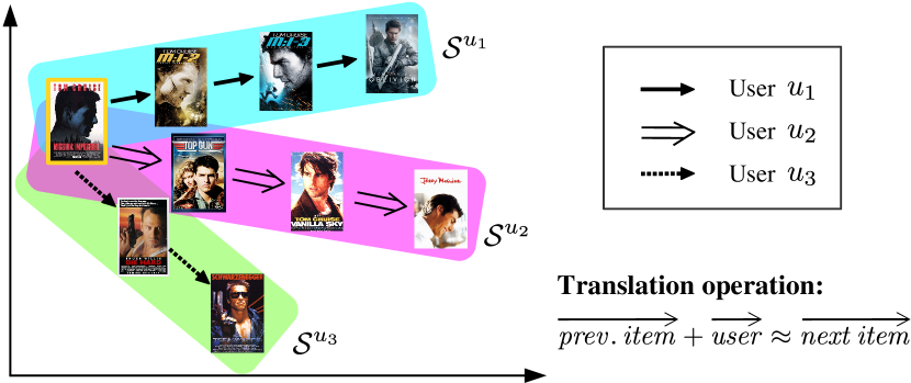
Figure 1. TransRec as a sequential model: Items (movies) are embedded into a ‘transition space’ where each user is modeled by a translation vector. The transition of a user from one item to another is captured by a user-specific translation operation. Here we demonstrate the historical sequences $\mathcal{S}^{u_{1}}$, $\mathcal{S}^{u_{2}}$, and $\mathcal{S}^{u_{3}}$ of three users. Given the same starting point, the movie Mission: Impossible I, $u_{1}$ went on to watch the whole series, $u_{2}$ continued to watch drama movies by Tom Cruise, and $u_{3}$ switched to similar action movies.

Traditional recommendation methods usually excel at modeling two-way (i.e., pairwise) interactions. There are Matrix Factorization (MF) techniques (Koren et al., 2009) that make use of inner products to model the compatibility between user-item pairs (i.e., user preferences). Likewise, there are also (first-order) Markov Chain (MC) models (Serfozo, 2009) that capture transition relationships between pairs of adjacent items in sequences (i.e., sequential dynamics), often by way of factorizing the transition matrix in favor of generalization ability. For the task of sequential recommendation, researchers have made use of scalable tensor factorization methods, such as Factorized Personalized Markov Chains (FPMC) proposed by Rendle et al. (Rendle et al., 2010). FPMC models third-order relationships between $u$, $i$, and $j$ by the summation of two pairwise relationships: one for the compatibility between $u$ and the next item $j$, and another for the sequential continuity between the previous item $i$ and the next item $j$. Ultimately, this is a combination of MF and MC (see Section 3.5 for details).

Recently, there have been two lines of works that aim to improve FPMC. Personalized metric embedding methods replace the inner products in FPMC with Euclidean distances, where the metricity assumption—especially the triangle inequality—enables the model to generalize better (Wu et al., 2013; Moore et al., 2013; Feng et al., 2015). However, these works still adopt the framework of modeling the user preference component and sequential continuity component separately, which may be disadvantageous as the two components are inherently correlated.

Another line of work (Wang et al., 2015) makes use of operations like average/max pooling to aggregate the representations of the user $u$ and the previous item $i$, before their compatibility with the next item $j$ is measured. These works partially address the issue of modeling the dependence of the two key components, though are hard to interpret and can not benefit from the generalization ability of metric embeddings.

In this paper, we aim to tackle the above issues by introducing a new framework called Translation-based Recommendation (TransRec). The key idea behind TransRec is presented in Figure 1: Items are embedded as points in a (latent) ‘transition space’; each user is represented as a ‘translation vector’ in the same space. Then, the third-order interactions mentioned earlier are captured by a personalized translation operation: the coordinates of previous item $i$, plus the translation vector of $u$ determine (approximately) the coordinates of the next item $j$, i.e., $\vec{\gamma}_{i}+\vec{t}_{u}\approx\vec{\gamma}_{j}$. Finally, we model the compatibility of the $(u,i,j)$ triplet with a distance function $d(\vec{\gamma}_{i}+\vec{t}_{u},\vec{\gamma}_{j})$. At prediction time, recommendations can be via nearest-neighbor search centered at $\vec{\gamma}_{i}+\vec{t}_{u}$.

The advantages of such an approach are three-fold: (1) TransRec naturally models third-order interactions with only a single component; (2) TransRec also enjoys the generalization benefits from the implicit metricity assumption; and (3) TransRec can easily handle large sequences (e.g., millions of instances) due to its simple form. Empirically, we conduct comprehensive experiments on a wide range of large, real-world datasets (which are publicly available), and quantitatively demonstrate the superior recommendation performance achieved by TransRec.

In addition to the sequential prediction task, we also investigate the strength of TransRec at tackling item-to-item recommendation where pairwise relations between items need to be captured, e.g., suggesting a shirt to match a previously purchased pair of pants. State-of-the-art works for this task are mainly based on metric or non-metric embeddings (e.g., (He et al., 2016; McAuley et al., 2015)). We empirically evaluate TransRec on eight large co-purchase datasets from Amazon and find it to significantly outperform multiple state-of-the-art models by using the translation structure.

Finally, we introduce a new large, sequential prediction dataset, from Google Local, that contains a large corpus of ratings and reviews on millions of businesses around the world.

2. Related Work

General recommendation. Traditional approaches to recommendation ignore sequential signals in the system. Such systems focus on modeling user preferences, and typically rely on Collaborative Filtering (CF) techniques, especially Matrix Factorization (MF) (Ricci et al., 2011). For implicit feedback data (like purchases, clicks, and thumbs-up), point-wise and pairwise methods based on MF have been proposed. Point-wise methods (e.g., (Hu et al., 2008; Pan et al., 2008; Ning and Karypis, 2011)) assume all non-observed feedback to be negative and factorize the user-item feedback matrix. In contrast, pairwise methods (e.g., (Rendle et al., 2009; Rendle and Schmidt-Thieme, 2010; Rendle and Freudenthaler, 2014)) make a weaker assumption that users simply prefer observed feedback over unobserved feedback and optimize the pairwise rankings of (positive, non-positive) pairs.

Modeling temporal dynamics. Several works extend general recommendation models to make use of timestamps associated with feedback. For example, early similarity-based CF (e.g., (Ding and Li, 2005)) uses time weighting schemes that assign decaying weights to previously-rated items when computing similarities. More recent efforts are mostly based on MF, where the goal is to model and understand the historical evolution of users and items, e.g., Koren et al. achieved state-of-the-art rating prediction results on Netflix data, largely by exploiting temporal signals (Koren, 2010; Koren et al., 2009). The sequential prediction task we are tackling is related to the above, except that instead of directly using those timestamps, it focuses on learning the sequential relationships between user actions (i.e., it focuses on the order of actions rather than the specific time).

Sequential recommendation. Scalable sequential models usually rely on Markov Chains (MC) to capture sequential patterns (e.g., (Rendle et al., 2010; Wang et al., 2015; Feng et al., 2015)). Rendle et al. proposed to factorize the third-order ‘cube’ that represents the transitions amongst items made by users. The resulting model, Factorized Personalized Markov Chains (FPMC), can be seen as a combination of MF and MC and achieves good performance for next-basket recommendation.

There are also works that have adopted metric embeddings for the recommendation task, leading to better generalization ability. For example, Chen et al. introduced Logistic Metric Embeddings (LME) for music playlist generation (Chen et al., 2012), where the Markov transitions among different songs are encoded by the distances among them. Recently, Feng et al. further extended LME to model personalized sequential behavior and used pairwise ranking for predicting next points-of-interest (Feng et al., 2015). On the other hand, Wang et al. recently introduced the Hierarchical Representation Model (HRM), which extends FPMC by applying aggregation operations (like max/average pooling) to model more complex interactions. We will give more details of these works in Section 3.5.2.

Our work differs from the above in that we introduce a translation-based structure which naturally models the third-order interactions between a user, the previous item, and the next item for personalized Markov transitions.

Table 1. Notation

Notation	Explanation
$\mathcal{U}$, $\mathcal{I}$	user set, item set
$u$, $i$, $j$	user $u\in\mathcal{U}$, items $i,j\in\mathcal{I}$
$\mathcal{S}^{u}$	historical sequence of user $u$: $(\mathcal{S}^{u}_{1},\mathcal{S}^{u}_{2},\cdots,\mathcal{S}^{u}_{|\mathcal{S}^{u}|})$
$\Phi$	transition space; $\Phi=\mathbb{R}^{K}$
$\Psi$	a subspace in $\Phi$; $\Psi\subseteq\Phi$
$\vec{\gamma}_{i}$	embedding vector associated with item $i$; $\vec{\gamma}_{i}\in\Psi$
$\vec{t}$	(global) translation vector $\vec{t}\in\Phi$
$\vec{t}_{u}$	translation vector associated with user $u$; $\vec{t}_{u}\in\Phi$
$\vec{T}_{u}$	$\vec{T}_{u}=\vec{t}+\vec{t}_{u}$; $\vec{T}_{u}\in\Phi$
$\beta_{i}$	bias term associated with item $i$; $\beta_{i}\in\mathbb{R}$
$\vec{f}_{i}$	explicit feature vectors associated with item $i$
$d(x,y)$	distance between $x$ and $y$

Knowledge bases. Although different from recommendation, there has been a large body of work in knowledge bases that focuses on modeling multiple, complex relationships between various entities. Recently, partially motivated by the findings made by word2vec (Mikolov et al., 2013), translation-based methods (e.g., (Bordes et al., 2013; Lin et al., 2015; Wang et al., 2014)) have achieved state-of-the-art accuracy and scalability, in contrast to those achieved by traditional embedding methods relying on tensor decomposition or collective matrix factorization (e.g., (Nickel et al., 2011, 2012; Singh and Gordon, 2008)). Our work is inspired by those findings, and we tackle the challenges from modeling large-scale, personalized, and complicated sequential data. This is the first work that explores this direction to the best of our knowledge.

3. The Translation-based Model

3.1. Problem Formulation

We refer to the objects that users ($\mathcal{U}$) interact with in the system as items ($\mathcal{I}$), e.g., products, movies, or places. The sequential, or ‘next-item,’ prediction task we are tackling is formulated as follows. For each user $u\in\mathcal{U}$ we have a sequence of items $\mathcal{S}^{u}=(\mathcal{S}^{u}_{1},\mathcal{S}^{u}_{2},\cdots,\mathcal{S}^{u}_{|\mathcal{S}^{u}|})$ that $u$ has interacted with. Given the sequence set from all users $\mathcal{S}=\{\mathcal{S}^{u_{1}},\mathcal{S}^{u_{2}},\cdots,\mathcal{S}^{u_{|\mathcal{U}|}}\}$, our objective is to predict the next item to be ‘consumed’ by each user and generate recommendation lists accordingly. Notation used throughout the paper is summarized in Table 1.

3.2. The Proposed Model

We aim to build a model that (1) naturally captures personalized sequential behavior, and (2) easily scales to large, real-world datasets. Methodologically, we learn a transition space $\Phi=\mathbb{R}^{K}$, where each item $i$ is represented with a point/vector $\vec{\gamma}_{i}\in\Phi$. $\vec{\gamma}_{i}$ can be latent, or transformed from certain explicit features of item $i$, e.g., the output of a neural network. In this paper we take $\vec{\gamma}_{i}$ as latent vectors.

Recall that the historical sequence $\mathcal{S}^{u}$ of user $u$ is a series of transitions $u$ has made from one item to another. To model the personalized sequential behavior, we represent each user $u$ with a translation vector $\vec{t_{u}}\in\Phi$ to capture $u$’s inherent intent or ‘long-term preferences’ that influenced her to make these decisions. In particular, if $u$ transitioned from item $i$ to item $j$, what we want is

$$\vec{\gamma}_{i}+\vec{t}_{u}\approx\vec{\gamma}_{j},$$

which means $\vec{\gamma}_{j}$ should be a nearest neighbor of $\vec{\gamma}_{i}+\vec{t}_{u}$ in $\Phi$ according to some distance metric $d(x,y)$, e.g., $\mathcal{L}_{1}$ distance.

Note that we are uncovering a metric space where (1) neighborhood captures the notion of similarity and (2) translation encapsulates various semantically complex transition relationships amongst items. In both cases, the inherent triangle inequality assumption plays an important role in helping the model to generalize well, as it does in canonical metric learning scenarios. For instance, if users tend to transition from item A to two items B and C, then TransRec will also put B close to C. This is a desirable property especially when data sparsity is a major concern. One plausible alternative is to use the inner product of $\vec{\gamma}_{i}+\vec{t}_{u}$ and $\vec{\gamma}_{j}$ to model their ‘compatibility.’ However, this way item B and C in our above example might be far from each other because inner products do not guarantee the triangle inequality condition.

Due to the sparsity of real-world datasets, it might not be affordable to learn separate translation vectors $\vec{t}_{u}$ for each user. Therefore we add another translation vector $\vec{t}$ to capture ‘global’ transition dynamics across all users, and we let

$$\vec{T}_{u}=\vec{t}+\vec{t}_{u}.$$

This way $\vec{t}_{u}$ can be seen as an offset vector associated with user $u$. Although doing so yields no additional expressive power, the advantage is that $\vec{t}_{u}$’s of cold-start users will be regularized towards 0 and we are essentially using $\vec{t}$—the ‘average’ behavior—to make predictions for these users.

Finally, the probability that a given user $u$ transitions from the previous item $i$ to the next item $j$ is predicted by

(1) $$\mathit{Prob}(j~{}|~{}u,i)\propto\beta_{j}-d(\vec{\gamma}_{i}+\vec{T}_{u},\vec{\gamma}_{j}),$$

$$\text{subject to}\quad\vec{\gamma}_{i}\in\Psi\subseteq\Phi,\;\;\;\text{for}{\ }i\in\mathcal{I}.$$

$\Psi$ is a subspace in $\Phi$, e.g., a unit ball, a technique which has been shown to be helpful for mitigating ‘curse of dimensionality’ issues (e.g., (Bordes et al., 2013; Wang et al., 2014; Lin et al., 2015)). In the above equation a single bias term $\beta_{j}$ is added to capture overall item popularity.

Ranking Optimization. Given a user and the associated historical sequence, the ultimate goal of the task is to rank the ground-truth item $j$ higher than all other items ($j^{\prime}\in\mathcal{I}\setminus j$). Therefore it is a natural choice to optimize the pairwise ranking between $j$ and $j^{\prime}$ by (e.g.) Sequential Bayesian Personalized Ranking (S-BPR) (Rendle et al., 2010). To this end, we optimize the total order $>_{u,i}$ given the user $u$ and the previous item $i$ in the sequence:

(2) $$\begin{split}\widehat{\Theta}&=\operatorname*{arg\,max}_{\Theta}~{}\ln\prod_{u\in\mathcal{U}}\prod_{j\in\mathcal{S}^{u}}\prod_{j^{\prime}\notin\mathcal{S}^{u}}\mathit{Prob}(j>_{u,i}j^{\prime}|\Theta)~{}\mathit{Prob}(\Theta)\\ &=\operatorname*{arg\,max}_{\Theta}~{}\sum_{u\in\mathcal{U}}\sum_{j\in\mathcal{S}^{u}}\sum_{j^{\prime}\notin\mathcal{S}^{u}}\ln\sigma(\widehat{p}_{u,i,j}-\widehat{p}_{u,i,j^{\prime}})-\Omega(\Theta),\end{split}$$

where $i$ is the preceding item of $j$ in $\mathcal{S}^{u}$, $\widehat{p}_{u,i,j}$ is a shorthand for the prediction in Eq. (1), $\Theta$ is the parameter set $\{\beta_{i\in\mathcal{I}},\vec{\gamma}_{i\in\mathcal{I}},\vec{t}_{u\in\mathcal{U}},\vec{t}\}$, and $\Omega(\Theta)$ is an $\mathcal{L}_{2}$ regularizer. Note that according to S-BPR, the probability that the ground-truth item $j$ is ranked higher than a ‘negative’ item $j^{\prime}$ (i.e., $\mathit{Prob}(j>_{u,i}j^{\prime}|\Theta)$) is estimated by the sigmoid function $\sigma(\widehat{p}_{u,i,j}-\widehat{p}_{u,i,j^{\prime}})$.

3.3. Inferring the Parameters

Initialization. Item embeddings $\vec{\gamma}_{i\in\mathcal{I}}$ and $\vec{t}$ are randomly initialized to be unit vectors. $\beta_{i\in\mathcal{I}}$ and $\vec{t}_{u\in\mathcal{U}}$ are initialized to be zero.

Learning Procedure. The objective function (Eq. (2)) is maximized by stochastic gradient ascent: First, we uniformly sample a user $u$ from $\mathcal{U}$. Then, a ‘positive’ item $j$ and a ‘negative’ item $j^{\prime}$ are uniformly sampled from $\mathcal{S}^{u}\setminus\mathcal{S}^{u}_{1}$ and $\mathcal{I}\setminus\mathcal{S}^{u}$ respectively. Next, parameters are updated via stochastic gradient ascent:

$$\Theta\leftarrow\Theta+\epsilon\cdot\left(\sigma(\widehat{p}_{u,i,j^{\prime}}-\widehat{p}_{u,i,j})~{}\frac{\partial(\widehat{p}_{u,i,j}-\widehat{p}_{u,i,j^{\prime}})}{\partial\Theta}-\lambda_{\Theta}\cdot\Theta\right),$$

where $\epsilon$ is the learning rate and $\lambda_{\Theta}$ is a regularization hyperparameter. Finally, we re-normalize $\vec{\gamma}_{i}$, $\vec{\gamma}_{j}$, and $\vec{\gamma}_{j^{\prime}}$ to be vectors in $\Psi$. For example, if we let $\Psi$ be the unit $\mathcal{L}_{2}$-ball, then $\vec{\gamma}\leftarrow\vec{\gamma}/\text{max}(1,\|\vec{\gamma}\|)$. The above steps are repeated until convergence or until the accuracy plateaus on the validation set.

3.4. Nearest Neighbor Search

At test time, recommendation can be made via nearest neighbor search. A small challenge lies in handling bias terms: First, we replace $\beta_{j}$ with $\beta^{\prime}_{j}=\beta_{j}-\max_{k\in\mathcal{I}}\beta_{k}$ for $j\in\mathcal{I}$. Shifting the bias terms does not change the ranking of items for any query. Next, we absorb $\beta^{\prime}_{j}$ into $\vec{\gamma}_{j}$ and get $\vec{\gamma}^{\prime}_{j}=(\vec{\gamma}_{j};\sqrt{-\beta^{\prime}_{j}})$ for (squared) $\mathcal{L}_{2}$ distance, or $\vec{\gamma}^{\prime}_{j}=(\vec{\gamma}_{j};\beta^{\prime}_{j})$ for $\mathcal{L}_{1}$ distance. Finally, given a user $u$ and an item $i$, we obtain the ‘query’ coordinate $(\vec{\gamma}_{i}+\vec{T}_{u};0)$, which can then be used for retrieving nearest neighbors in the space of $\vec{\gamma}^{\prime}_{j}$.

3.5. Connections to Existing Models

3.5.1. Knowledge Graphs

Our method is inspired by recent advances in knowledge graph completion, e.g., (Bordes et al., 2013; Wang et al., 2014; Lin et al., 2015; Yang et al., 2015; Trouillon et al., 2016), where the objective is to model multiple types of relations between pairs of entities, e.g., Turing was born in England (‘was_born_in’ is the relation between ‘Turing’ and ‘England’). One state-of-the-art technique (e.g., (Bordes et al., 2013; Wang et al., 2014; Lin et al., 2015)) is embedding entities as points and relations as translation vectors such that the relationship between two entities is captured by the corresponding translation operation. In the previous example, if we represent ‘Turing,’ ‘England,’ and ‘was_born_in’ with vectors $\overrightarrow{\mathit{head}}$, $\overrightarrow{\mathit{tail}}$, and $\overrightarrow{\mathit{relation}}$ respectively, then the following is desired: $\overrightarrow{\mathit{head}}+\overrightarrow{\mathit{relation}}\approx\overrightarrow{\mathit{tail}}$.

In recommendation settings, items are analogous to ‘entities’ in knowledge graphs. Our key idea is to represent each user as one particular type of ‘relation’ such that it captures the personalized reasons a user transitions from one item to another.

3.5.2. Sequential Models

State-of-the-art sequential prediction models are typically based on (personalized) Markov Chains. FPMC is a seminal model proposed by (Rendle et al., 2010), whose predictor consists of two key components: (1) the inner product of user and item factors (capturing users’ inherent preferences), and (2) the inner product of the factors of the previous and next item (capturing sequential dynamics). FPMC is essentially the combination of MF and factorized MC:

(3) $$\mathit{Prob}(j~{}|~{}u,i)\propto\langle\vec{M}_{u},\vec{N}_{j}\rangle+\langle\vec{P}_{i},\vec{Q}_{j}\rangle,$$

where user embeddings $\vec{M}_{u}$ and item embeddings $\vec{N}_{j}$, $\vec{P}_{i}$, $\vec{Q}_{j}$ are parameters learned from the data.

Recently, Personalized Ranking Metric Embedding (PRME) (Feng et al., 2015) was proposed to improve FPMC by learning two metric spaces: one for measuring user-item affinity and another for sequential continuity. It predicts according to:

(4) $$\mathit{Prob}(j~{}|~{}u,i)\propto-\;\left(\alpha\cdot\|\vec{M}_{u}-\vec{N}_{j}\|_{2}^{2}~{}+~{}(1-\alpha)\cdot\|\vec{P}_{i}-\vec{P}_{j}\|_{2}^{2}\right),$$

which replaces inner products in FPMC by distances. As argued in (Chen et al., 2012; Feng et al., 2015), the underlying metricity assumption brings better generalization ability. However, like FPMC, PRME still has to learn two closely correlated components in a separate manner, using a hyperparameter $\alpha$ to balance them.

Another recent work, Hierarchical Representation Model (HRM) (Wang et al., 2015), tries to extend FPMC by using an aggregation operation (max/average pooling) to blend users’ preferences ($\vec{M}_{u}$) and their recent activities ($\vec{N}_{i}$):

(5) $$\mathit{Prob}(j~{}|~{}u,i)\propto\langle\text{aggregation}(\vec{M}_{u},\vec{N}_{i}),\vec{N}_{j}\rangle.$$

Although the predictor can be seen as modeling the third-order interactions with a single component, the aggregation is hard to interpret and does not reap the benefits of using metric embeddings as PRME does.

TransRec also falls into the category of Markov Chain models; however, it applies a novel translation-based structure in a metric space, which enjoys the benefits of using a single, interpretable component as well as a metric space.

4. Experiments

4.1. Datasets and Statistics

To fully evaluate the capability and applicability of TransRec, in our experiments we include a wide range of publicly available datasets varying significantly in domain, size, data sparsity, and variability/complexity.

Table 2. Statistics (in ascending order of item density).

Dataset	#users ($|\mathcal{U}|$)	#items ($|\mathcal{I}|$)	#actions	avg. #actions /user	avg. #actions /item
Epinions	5,015	8,335	26,932	5.37	3.23
Automotive	34,316	40,287	183,573	5.35	4.56
Google	350,811	505,516	2,591,026	7.39	5.13
Office	16,716	22,357	128,070	7.66	5.73
Toys	57,617	69,147	410,920	7.13	5.94
Clothing	184,050	174,484	1,068,972	5.81	6.13
Cellphone	68,330	60,083	429,231	6.28	7.14
Games	31,013	23,715	287,107	9.26	12.11
Electronics	253,996	145,199	2,109,879	8.31	14.53
Foursquare	43,110	13,335	306,553	7.11	22.99
Flixter	69,485	25,759	8,000,971	115.15	310.61
Total	1.11M	1.09M	15.5M	-	-

Amazon. The first group of datasets, comprising large corpora of reviews and timestamps on various products, were recently introduced by (McAuley et al., 2015). These data are originally from Amazon.com and span May 1996 to July 2014. Top-level product categories on Amazon were constructed as separate datasets by (McAuley et al., 2015). In this paper, we take a series of large categories including ‘Automotive,’ ‘Cell Phones and Accessories,’ ‘Clothing, Shoes, and Jewelry,’ ‘Electronics,’ ‘Office Products,’ ‘Toys and Games,’ and ‘Video Games.’ This set of data is notable for its high sparsity and variability.

Epinions. This dataset was collected by (Zhao et al., 2014) from Epinions.com, a popular online consumer review website. The reviews span January 2001 to November 2013.

Foursquare. Is originally from Foursquare.com, containing a large number of check-ins of users at different venues from December 2011 to April 2012. This dataset was collected by (Levandoski et al., 2012) and is widely used for evaluating next point-of-interest prediction methods.

Flixter. A large, dense movie rating dataset from Flixter.com. The timespan is from November 2005 to November 2009.

Google Local. We introduce a new dataset from Google which contains 11,453,845 reviews and ratings from 4,567,431 users on 3,116,785 local businesses (with detailed name, hours, phone number, address, GPS, etc.). There are as many as 48,013 categories of local businesses distributed over five continents, ranging from restaurants, hotels, parks, shopping malls, movie theaters, schools, military recruiting offices, bird control, mediation services (etc.). Figure 2 shows the number of reviews and businesses associated with each of the top 1,000 popular categories. The vast vocabulary of items, variability, and data sparsity make it a challenging dataset to examine the effectiveness of our model. Although not the goal of our study, this is also a potentially useful dataset for location-based recommendation.

For each of the above datasets, we discard users and items with fewer than 5 associated actions in the system. In cases where star-ratings are available, we take all of them as users’ positive feedback, since we are dealing with implicit feedback settings and care about purchases/check-in actions (etc.) rather than the specific ratings. Statistics of our datasets (after pre-processing) are shown in Table 2.

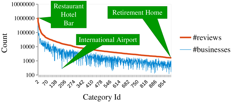
Figure 2. Number of reviews and local businesses associated with the top 1,000 popular categories from Google Local.

4.2. Comparison Methods

PopRec: This is a naïve baseline that ranks items according to their popularity, i.e., it recommends the most popular items to users and is not personalized.

Bayesian Personalized Ranking (BPR-MF) (Rendle et al., 2009): BPR-MF is a state-of-the-art item recommendation model which takes Matrix Factorization as the underlying predictor. It ignores the sequential signals in the system.

Factorized Markov Chain (FMC): Captures the ‘global’ sequential dynamics by factorizing the item-to-item transition matrix (shared by all users), but does not capture personalized behavior.

Factorized Personalized Markov Chain (FPMC) (Rendle et al., 2010): Uses a predictor that combines Matrix Factorization and factorized Markov Chains so that personalized Markov behavior can be captured (see Eq. (3)).

Personalized Ranking Metric Embedding (PRME) (Feng et al., 2015): PRME models personalized Markov behavior by the summation of two Euclidean distances (see Eq. (4)).

Hierarchical Representation Model (HRM) (Wang et al., 2015): HRM extends FPMC by using aggregation operations like max pooling to model more complex interactions (see Eq. (5)). We compare against HRM with both max pooling and average pooling, denoted by HRM${}_{\text{max}}$ and HRM${}_{\text{avg}}$ respectively.

Translation-based Recommendation (TransRec): Our method, which unifies user preferences and sequential dynamics with translations. In experiments we try both $\mathcal{L}_{1}$ and squared $\mathcal{L}_{2}$ distance for our predictor (see Eq. (1)).

Table 3 examines the properties of different methods. The ultimate goal of the baselines is to demonstrate (1) the performance achieved by state-of-the-art sequentially-unaware item recommendation models (BPR-MF) and purely sequential models without modeling personalization (FMC); (2) the benefits of combining personalization and sequential dynamics in a ‘linear’ (FPMC) and non-linear way (HRM), or using metric embeddings (PRME); and (3) the strength of TransRec using translations.

4.3. Evaluation Methodology

For each dataset, we partition the historical sequence $\mathcal{S}^{u}$ for each user $u$ into three parts: (1) the most recent one $\mathcal{S}^{u}_{|\mathcal{S}^{u}|}$ for test, (2) the second most recent one $\mathcal{S}^{u}_{|\mathcal{S}^{u}|-1}$ for validation, and (3) all the rest for training. Hyperparameters in all cases are tuned by grid search with the validation set. Finally, we report the performance of each method on the test set in terms of the following ranking metrics:

Area Under the ROC Curve (AUC):

$$\mathit{AUC}=\frac{1}{|\mathcal{U}|}\sum_{u\in\mathcal{U}}\frac{1}{|\mathcal{I}\setminus\mathcal{S}^{u}|}\sum_{j^{\prime}\in\mathcal{I}\setminus\mathcal{S}^{u}}\mathbf{1}(R_{u,g_{u}}<R_{u,j^{\prime}}),$$

Hit Rate at position 50 (Hit@50):

$$\mathit{Hit@50}=\frac{1}{|\mathcal{U}|}\sum_{u\in\mathcal{U}}\mathbf{1}(R_{u,g_{u}}\leq 50),$$

where $g_{u}$ is the ‘ground-truth’ item associated with user $u$ at the most recent time step, $R_{u,i}$ is the rank of item $i$ for user $u$ (smaller is better), and $\mathbf{1}(b)$ is an indicator function that returns $1$ if the argument $b$ is $\mathit{true}$; $0$ otherwise.

Table 3. Models. P: Personalized? S: Sequentially-aware? M: Metric-based? U: Unified model of third-order relations?

Property	PopRec	BPR-MF	FMC	FPMC	HRM	PRME	TransRec
P	✘	✔	✘	✔	✔	✔	✔
S	✘	✘	✔	✔	✔	✔	✔
M	✘	✘	✘	✘	✘	✔	✔
U	✘	✘	✘	✘	✔	✘	✔

Table 4. Ranking results on different datasets (higher is better). The number of latent dimensions $K$ for all comparison methods is set to 10. The best performance in each case is underlined. The last column shows the percentage improvement of TransRec over the best baseline.

Dataset	Metric	PopRec	BPR-MF	FMC	FPMC	HRM${}_{\text{avg}}$	HRM${}_{\text{max}}$	PRME	TransRec${}_{\mathcal{L}_{1}}$	TransRec${}_{\mathcal{L}_{2}}$	%Improv.
Epinions	AUC	0.4576	0.5523	0.5537	0.5517	0.6060	0.5617	0.6117	0.6063	0.6133	0.3%
	Hit@50	3.42%	3.70%	3.84%	2.93%	3.44%	2.79%	2.51%	3.18%	4.63%	20.6%
Automotive	AUC	0.5870	0.6342	0.6438	0.6427	0.6704	0.6556	0.6469	0.6779	0.6868	2.5%
	Hit@50	3.84%	3.80%	2.32%	3.11%	4.47%	3.71%	3.42%	5.07%	5.37%	20.1%
Google	AUC	0.5391	0.8188	0.7619	0.7740	0.8640	0.8102	0.8252	0.8359	0.8691	0.6%
	Hit@50	0.32%	4.27%	3.54%	3.99%	3.55%	4.59%	5.07%	6.37%	6.84%	32.5%
Office	AUC	0.6427	0.6979	0.6867	0.6866	0.6981	0.7005	0.7020	0.7186	0.7302	4.0%
	Hit@50	1.66%	4.09%	2.66%	2.97%	5.50%	4.17%	6.20%	6.86%	6.51%	10.7%
Toys	AUC	0.6240	0.7232	0.6645	0.7194	0.7579	0.7258	0.7261	0.7442	0.7590	0.2%
	Hit@50	1.69%	3.60%	1.55%	4.41%	5.25%	3.74%	4.80%	5.46%	5.44%	4.0%
Clothing	AUC	0.6189	0.6508	0.6640	0.6646	0.7057	0.6862	0.6886	0.7047	0.7243	2.6%
	Hit@50	1.11%	1.05%	0.57%	0.51%	1.70%	1.15%	1.00%	1.76%	2.12%	24.7%
Cellphone	AUC	0.6959	0.7569	0.7347	0.7375	0.7892	0.7654	0.7860	0.7988	0.8104	2.7%
	Hit@50	4.43%	5.15%	3.23%	2.81%	8.77%	6.32%	6.95%	9.46%	9.54%	8.8%
Games	AUC	0.7495	0.8517	0.8407	0.8523	0.8776	0.8566	0.8597	0.8711	0.8815	0.4%
	Hit@50	5.17%	10.93%	13.93%	12.29%	14.44%	12.86%	14.22%	16.61%	16.44%	15.0%
Electronics	AUC	0.7837	0.8096	0.8158	0.8082	0.8212	0.8148	0.8337	0.8457	0.8484	1.8%
	Hit@50	4.62%	2.98%	4.15%	2.82%	4.09%	2.59%	3.07%	4.89%	5.19%	12.3%
Foursquare	AUC	0.9168	0.9511	0.9463	0.9479	0.9559	0.9523	0.9565	0.9631	0.9651	0.9%
	Hit@50	55.60%	60.03%	63.00%	64.53%	60.75%	61.60%	65.32%	66.12%	67.09%	2.7%
Flixter	AUC	0.9459	0.9722	0.9568	0.9718	0.9695	0.9687	0.9728	0.9727	0.9750	0.2%
	Hit@50	11.92%	21.58%	22.23%	33.11%	32.34%	30.88%	40.81%	35.52%	35.02%	-13.0%

4.4. Performance and Quantitative Analysis

Results are collated in Table 4. Due to the sparsity of most of the datasets in consideration, the number of dimensions $K$ of all latent vectors in all cases is set to 10 for simplicity; we investigate the importance of the number of dimensions in our parameter study later. Note that in Table 4 datasets are ranked in ascending order of item density. The last column (%Improv.) demonstrates the percentage improvement of TransRec over the strongest baseline for each dataset. The main findings are summarized as follows:

BPR-MF and FMC achieve considerably better results than the popularity-based baseline in most cases, in spite of modeling personalization and sequential patterns in isolation. This means that uncovering the underlying user-item and item-item relationships is key to making meaningful recommendations.

FPMC and HRM are essentially combinations of MF and FMC. FPMC beats BPR-MF and FMC mainly on relatively dense datasets like Toys, Foursquare, and Flixter, and loses on sparse datasets—possibly due to the large number of parameters it introduces. From Table 4 we see that HRM achieves strong results amongst all baselines in most cases, presumably from the aggregation operations.

PRME replaces the inner products in FPMC by distance functions. It beats FPMC in most cases, though loses to HRM due to different modeling strategies. Note that like FPMC, PRME turns out to be quite strong at handling dense datasets like Foursquare and Flixter. We speculate that the two models could benefit from the considerable amount of additional parameters they use when data is dense.

TransRec outperforms other methods in nearly all cases. The improvements seem to be correlated with:

Variability. TransRec achieves large improvements (32.5% and 24.7% in terms of Hit@50) on Google and Clothing, two datasets with the largest vocabularies of items in our collection. Taking Google as an example, it includes all kinds of restaurants, bars, shops (etc.) as well as a global user base, which requires the ability to handle the vast variability.

Sparsity. TransRec beats all baselines especially on comparatively sparser datasets like Epinions, Automotive, and Google. The only exception is in terms of Hit@50 on Flixter, the densest dataset in consideration. We speculate that TransRec is at a disadvantage by using fewer parameters (than PRME) especially when $K$ is set to a small number (10). As we demonstrate in Section 4.6, we can achieve comparable results with the strongest baseline when increasing the model dimensionality.

In addition, we empirically find that (squared) $\mathcal{L}_{2}$ distance typically outperforms $\mathcal{L}_{1}$ distance, though the latter also beats baselines in most cases.

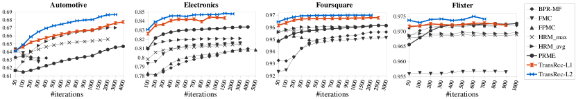
Figure 3. Convergence: Test AUCs on four datasets as the number of training iterations increases ($K=10$).

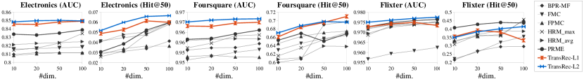
Figure 4. Sensitivity: Accuracy variation on the three densest datasets with increasing dimensionality (i.e., $K$).

4.5. Convergence

In Figure 3 we demonstrate (test) AUCs with increasing training iterations on four datasets with varying sparsity—Automotive, Electronics, Foursquare, and Flixter. Automotive is representative of sparse datasets in our collection. Simple baselines like FMC and BPR-MF converge faster than other methods on sparse datasets, presumably due to the relatively simpler dynamics they capture. FPMC also converges fast on such datasets as a result of its tendency to overfit (recall that we terminate once no further improvements are achieved on the validation set). On denser datasets like Electronics, Foursquare, and Flixter, all methods tend to converge at comparable speeds due to the need to unravel denser relationships amongst different entities.

4.6. Sensitivity

For the three densest datasets—Electronics, Foursquare, and Flixter—we also experimented with different numbers of dimensions for user/item representations. We increase $K$ from 10 to 100 and present AUC and Hit@50 values on the test set in Figure 4. TransRec still dominates other methods on Electronics and Foursquare. As for Flixter, from the rightmost subfigure we can see that in terms of Hit@50 the gap between TransRec ($\mathcal{L}_{2}$) and PRME, the strongest baseline on this data, closes as we increase the dimensionality.

4.7. Implementation Details

To make fair comparisons, we used stochastic gradient ascent to optimize pairwise rankings for all models (except PopRec) with a fixed learning rate of 0.05. Regularization hyperparamters are selected from $\{0,0.001,0.01,0.1,1\}$ (using the validation set). We did not make use of the dropout technique mentioned in the HRM paper to make it comparable to other methods. For PRME, we selected $\alpha$ from $\{0.2,0.5,0.8\}$. 0.2 was found to be the best in the PRME paper, which is consistent with our own observations. For TransRec, we used the unit $\mathcal{L}_{2}$-ball as our subspace $\Psi$. We also tried using the unit $\mathcal{L}_{2}$-sphere (i.e., the surface of the ball), but it led to slightly worse results in practice.

4.8. Recommendations

In Figure 5 we demonstrate some recommendations made by TransRec ($K=10$) on Electronics. We randomly sample a few users from the datasets and show their historical sequences on the left, and demonstrate the top-1 recommendation on the right. As we can see from these examples, TransRec can capture long-term dynamics successfully. For example, TransRec recommends a tripod to the first user who appears to be a photographer. The last user bought multiple headphones and similar items in history; TransRec recommends new headphones after the purchase of an iPod accessory. In addition, TransRec also captures short-term dynamics. For instance, it recommends a desktop case to the fifth user after the purchase of a motherboard. Similarly, the sixth user is recommended a HDTV after recently purchasing a home theater receiver/speaker.

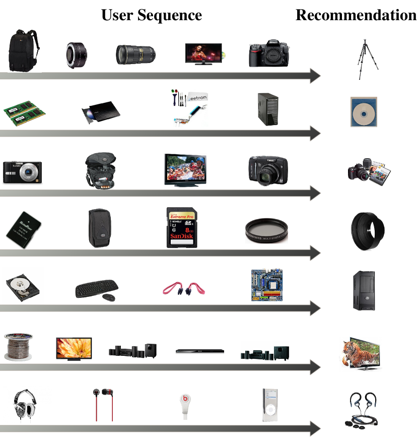
Figure 5. Recommendations made for a random sample of seven users by TransRec on Electronics data.

4.9. Item-to-item recommendation

By removing the personalization element, TransRec can straightforwardly be adapted to handle item-to-item recommendation, another classical setting where recommendations are made in the context of a specific item, e.g., recommending items that are likely to be purchased together. This setting is analogous to the knowledge graph completion task in that relationships among different items need to be modeled.

4.9.1. Datasets and Evaluation Methodology

We use 8 large datasets representing co-purchase relationships between products from Amazon (McAuley et al., 2015). They are a variety of top-level Amazon categories; to make the task more challenging, we only consider edges that connect two different top-level subcategories within each of the above datasets (e.g., recommending complementary items rather than substitutes). Statistics of these datasets are collated in Table 5.

Note that in these datasets edges are directed, e.g., it makes sense to recommend a charger/backpack after a customer purchases a laptop, but not the other way around.

Features. To further evaluate TransRec, we consider testing its capability here as a content-based method. To this end, we extract Bag-of-Words (BoW) features from each product’s review text. In short, for each dataset we removed stop-words and constructed a dictionary comprising the 5,000 most frequent nouns or adjectives or adjective-noun bigrams. These features have been shown to be effective on this data (He et al., 2016).

Table 5. Statistics (in ascending order of #edges).

Dataset	Full name	#items	#edges
Office	Office Products	130,006	52,942
Home	Home & Kitchen	410,244	122,955
Games	Video Games	50,210	314,124
Electronics	Electronics	476,004	549,914
Automotive	Automotive	320,116	637,814
Movies & TV	Movies & TV	200,941	648,256
Cellphone	Cell Phones & Accessories	319,678	667,918
Toys	Toys & Games	327,699	948,729
Total		2.23M	3.94M

Evaluation Methodology. For each of the above datasets, we randomly partition the edges with an 80%/10%/10% train/validation/test split. Validation is used to select hyperparameters and performance is reported on the test set. Again we report AUC and Hit@10 (see Section 4.3). Here we use 10 for the hit rate because, as we show later, item-to-item recommendation proves simpler than personalized sequential prediction.

4.9.2. The Translation-based Model

Here we adopt a content-based version of TransRec, to investigate its ability to tackle explicit features. Let $\vec{f}_{i}$ denote the explicit feature vector associated with item $i$. We add one additional embedding layer $E(\cdot)$ on top of $\vec{f}$ to project items into the ‘relational space’ $\Phi$. Formally, TransRec makes predictions according to

$$\mathit{Prob}(j~{}|~{}i)\propto-\;d\left(E(\vec{f}_{i})+\vec{t},E(\vec{f}_{j})\right),$$

$$\text{subject to}\quad E(\vec{f}_{i})\in\Psi\subseteq\Phi,\;\;\;\text{for}{\ }i\in\mathcal{I}.$$

$E(\cdot)$ could be a linear embedding layer, a non-linear layer like a neural network, or even some combination of latent and content-based representations.

4.9.3. Baselines

We mainly compare against two related models based on metric (or non-metric) embeddings. These are state-of-the-art content-based methods for item-to-item recommendation and have demonstrated strong results on the same data (McAuley et al., 2015; He et al., 2016). The complete list of baselines is as follows:

Weighted Nearest Neighbor (WNN): WNN measures the ‘dissimilarity’ between pairs of items by a weighted Euclidean distance in the raw feature space: $d_{\vec{w}}(i,j)=\|\vec{w}\circ(\vec{f}_{i}-\vec{f}_{j})\|_{2}^{2}$, where $\circ$ is the Hadamard product and $\vec{w}$ is a parameter to be learned.

Low-rank Mahalanobis Transform (LMT) (McAuley et al., 2015): A state-of-the-art embedding method for learning the notion of compatibilities among different items. LMT learns a single low-rank Mahalanobis transform matrix $W$ to embed all items into a relational space within which the distance between items is measured to make predictions: $d_{W}(i,j)=\|W\vec{f}_{i}-W\vec{f}_{j}\|_{2}^{2}$.

Mixtures of Non-metric Embeddings (Monomer) (He et al., 2016): Monomer extends LMT by learning mixtures of low-rank embeddings to uncover more complex reasons to explain the relationships between items. It relaxes the metricity assumption used by LMT and can naturally handle directed relationships.

4.9.4. Quantitative Results and Analyses

For fair comparison, we adopted the setting in (He et al., 2016), so that we use 100 dimensions for the relational spaces of LMT and TransRec; 5 spaces each with 20 dimensions are learned for Monomer. For simplicity, in our experiments we used squared $\mathcal{L}_{2}$ distance and $\Psi=\Phi$ for TransRec, i.e., no constraints on the vector $E(\vec{f})$. Also, a linear embedding layer is used as the function $E$ to make it more comparable with our baselines.

Experimental results are collated in Table 6. Our main findings are summarized as follows: (1) TransRec outperforms all baselines in all cases considerably, which indicates that translation-based structure seems to be stronger at modeling relationships among items compared to purely distance-based methods. This is also consistent with the findings from knowledge base literature (e.g., (Bordes et al., 2013; Wang et al., 2014; Lin et al., 2015)). (2) TransRec tends to lead to larger improvements for sparse datasets like Office, in contrast to the improvements on denser datasets like Toys and Games.

Table 6. Accuracy for co-purchase prediction (higher is better).

Dataset	Metric	WNN	LMT	Monomer	TransRec	%Improv.
Office	AUC	0.6952	0.8848	0.8736	0.9437	6.7%
	Hit@10	1.45%	3.08%	1.96%	12.69%	312.0%
Home	AUC	0.6696	0.9101	0.8841	0.9482	4.2%
	Hit@10	2.24%	4.46%	0.63%	8.80%	97.3%
Games	AUC	0.7199	0.9423	0.9239	0.9736	3.3%
	Hit@10	2.64%	4.19%	0.59%	7.78%	85.7%
Electronics	AUC	0.7538	0.9316	0.9299	0.9651	3.5%
	Hit@10	1.78%	2.59%	0.29%	5.32%	105.4%
Automotive	AUC	0.7317	0.9054	0.9152	0.9490	3.7%
	Hit@10	1.20%	1.97%	0.36%	4.48%	127.4%
Movies & TV	AUC	0.7668	0.9536	0.9516	0.9730	1.9%
	Hit@10	2.84%	4.37%	0.99%	6.19%	41.7%
Cellphone	AUC	0.6867	0.7932	0.8445	0.9127	8.1%
	Hit@10	0.80%	0.94%	0.04%	2.42%	157.5%
Toys	AUC	0.7529	0.9216	0.9353	0.9552	2.1%
	Hit@10	2.27%	2.67%	0.59%	3.99%	49.4%

5. Conclusion

We introduced a scalable translation-based method, TransRec, for modeling the semantically complex relationships between different entities in recommender systems. We analyzed the connections of TransRec to existing methods and demonstrated its suitability for modeling third-order interactions between users, their previously consumed item, and their next item. In addition to the superior results achieved on the sequential prediction task on a wide spectrum of large, real-world datasets, we also investigated the strength of TransRec at tackling item-to-item recommendation. The success of TransRec on the two tasks suggests that translation-based architectures are promising for general-purpose recommendation problems.

In addition, we introduced a large-scale dataset for sequential (and potentially geographical) recommendation from Google Local, that contains detailed information about millions of local businesses (e.g., restaurants, malls, shops) around the world as well as ratings and reviews from millions of users.

References

- (1)
- Bordes et al. (2013) Antoine Bordes, Nicolas Usunier, Alberto Garcia-Duran, Jason Weston, and Oksana Yakhnenko. 2013. Translating embeddings for modeling multi-relational data. In Proceedings of the Advances in Neural Information Processing Systems (NIPS). 2787–2795.
- Chen et al. (2012) Shuo Chen, Josh L. Moore, Douglas Turnbull, and Thorsten Joachims. 2012. Playlist prediction via metric embedding. In Proceedings of the ACM SIGKDD Conferences on Knowledge Discovery and Data Mining (SIGKDD). 714–722.
- Ding and Li (2005) Yi Ding and Xue Li. 2005. Time weight collaborative filtering. In Proceedings of the ACM International Conference on Information and Knowledge Management (CIKM). 485–492.
- Feng et al. (2015) Shanshan Feng, Xutao Li, Yifeng Zeng, Gao Cong, Yeow Meng Chee, and Quan Yuan. 2015. Personalized ranking metric embedding for next new POI recommendation. In Proceedings of the International Joint Conference on Artificial Intelligence (IJCAI). 2069–2075.
- He et al. (2016) Ruining He, Charles Packer, and Julian McAuley. 2016. Learning compatibility across categories for heterogeneous item recommendation. In IEEE International Conference on Data Mining (ICDM). 937–942.
- Hu et al. (2008) Yifan Hu, Yehuda Koren, and Chris Volinsky. 2008. Collaborative filtering for implicit feedback datasets. In Proceedings of the IEEE International Conference on Data Mining (ICDM). 263–272.
- Koren (2010) Yehuda Koren. 2010. Collaborative filtering with temporal dynamics. Commun. ACM 53, 4 (2010), 89–97.
- Koren et al. (2009) Yehuda Koren, Robert Bell, and Chris Volinsky. 2009. Matrix Factorization techniques for recommender systems. Computer 42, 8 (2009), 30–37.
- Levandoski et al. (2012) Justin J. Levandoski, Mohamed Sarwat, Ahmed Eldawy, and Mohamed F. Mokbel. 2012. LARS: A location-aware recommender system. In Proceedings of the IEEE International Conference on Data Engineering (ICDE). 450–461.
- Lin et al. (2015) Yankai Lin, Zhiyuan Liu, Maosong Sun, Yang Liu, and Xuan Zhu. 2015. Learning entity and relation embeddings for knowledge graph completion. In Proceedings of the AAAI Conference on Artificial Intelligence (AAAI). 2181–2187.
- McAuley et al. (2015) Julian J. McAuley, Christopher Targett, Qinfeng Shi, and Anton van den Hengel. 2015. Image-based recommendations on styles and substitutes. In Proceedings of the International ACM SIGIR Conference on Research and Development in Information Retrieval (SIGIR). 43–52.
- Mikolov et al. (2013) Tomas Mikolov, Ilya Sutskever, Kai Chen, Greg S Corrado, and Jeff Dean. 2013. Distributed representations of words and phrases and their compositionality. In Proceedings of the Advances in Neural Information Processing Systems (NIPS). 3111–3119.
- Moore et al. (2013) Joshua L. Moore, Shuo Chen, Douglas Turnbull, and Thorsten Joachims. 2013. Taste over time: the temporal dynamics of user preferences. In Proceedings of the International Society for Music Information Retrieval Conference (ISMIR). 401–406.
- Nickel et al. (2011) Maximilian Nickel, Volker Tresp, and Hans-Peter Kriegel. 2011. A three-way model for collective learning on multi-relational data. In Proceedings of the International Conference on Machine Learning (ICML). 809–816.
- Nickel et al. (2012) Maximilian Nickel, Volker Tresp, and Hans-Peter Kriegel. 2012. Factorizing yago: scalable machine learning for linked data. In Proceedings of the International Conference on World Wide Web (WWW). 271–280.
- Ning and Karypis (2011) Xia Ning and George Karypis. 2011. SLIM: Sparse linear methods for top-n recommender systems. In Proceedings of the IEEE International Conference on Data Mining (ICDM). 497–506.
- Pan et al. (2008) Rong Pan, Yunhong Zhou, Bin Cao, Nathan N. Liu, Rajan Lukose, Martin Scholz, and Qiang Yang. 2008. One-class collaborative filtering. In Proceedings of the IEEE International Conference on Data Mining (ICDM). 502–511.
- Rendle and Freudenthaler (2014) Steffen Rendle and Christoph Freudenthaler. 2014. Improving pairwise learning for item recommendation from implicit feedback. In Proceedings of the ACM International Conference on Web Search and Data Mining (WSDM). 273–282.
- Rendle et al. (2009) Steffen Rendle, Christoph Freudenthaler, Zeno Gantner, and Lars Schmidt-Thieme. 2009. BPR: Bayesian personalized ranking from implicit feedback. In Proceedings of the Conference on Uncertainty in Artificial Intelligence (UAI). 452–461.
- Rendle et al. (2010) Steffen Rendle, Christoph Freudenthaler, and Lars Schmidt-Thieme. 2010. Factorizing personalized markov chains for next-basket recommendation. In Proceedings of the International Conference on World Wide Web (WWW). 811–820.
- Rendle and Schmidt-Thieme (2010) Steffen Rendle and Lars Schmidt-Thieme. 2010. Pairwise interaction tensor factorization for personalized tag recommendation. In Proceedings of the ACM International Conference on Web Search and Data Mining (WSDM). 81–90.
- Ricci et al. (2011) Francesco Ricci, Lior Rokach, Bracha Shapira, and Paul Kantor. 2011. Recommender systems handbook. Springer US.
- Serfozo (2009) Richard Serfozo. 2009. Basics of applied stochastic processes. Springer Science & Business Media.
- Singh and Gordon (2008) Ajit P. Singh and Geoffrey J. Gordon. 2008. Relational learning via collective matrix factorization. In Proceedings of the ACM SIGKDD Conferences on Knowledge Discovery and Data Mining (SIGKDD). 650–658.
- Trouillon et al. (2016) Théo Trouillon, Johannes Welbl, Sebastian Riedel, Éric Gaussier, and Guillaume Bouchard. 2016. Complex embeddings for simple link prediction. In Proceedings of the International Conference on Machine Learning (ICML). 2071–2080.
- Wang et al. (2015) Pengfei Wang, Jiafeng Guo, Yanyan Lan, Jun Xu, Shengxian Wan, and Xueqi Cheng. 2015. Learning hierarchical representation model for nextbasket recommendation. In Proceedings of the International ACM SIGIR Conference on Research and Development in Information Retrieval (SIGIR). 403–412.
- Wang et al. (2014) Zhen Wang, Jianwen Zhang, Jianlin Feng, and Zheng Chen. 2014. Knowledge graph embedding by translating on hyperplanes. In Proceedings of the AAAI Conference on Artificial Intelligence (AAAI). 1112–1119.
- Wu et al. (2013) Xiang Wu, Qi Liu, Enhong Chen, Liang He, Jingsong Lv, Can Cao, and Guoping Hu. 2013. Personalized next-song recommendation in online karaokes. In Proceedings of the ACM Conference on Recommender Systems (RecSys). 137–140.
- Yang et al. (2015) Bishan Yang, Wen-tau Yih, Xiaodong He, Jianfeng Gao, and Li Deng. 2015. Embedding entities and relations for learning and inference in knowledge bases. In Proceedings of the International Conference on Learning Representations (ICLR). 1–13.
- Zhao et al. (2014) Tong Zhao, Julian McAuley, and Irwin King. 2014. Leveraging social connections to improve personalized ranking for collaborative filtering. In Proceedings of the ACM International Conference on Information and Knowledge Management (CIKM). 261–270.