Characterization of balls by generalized Riesz energy

Abstract

We show that balls, circles and $2$-spheres can be identified by generalized Riesz energy among compact submanifolds of the Euclidean space that are either closed or with codimension $0$, where the Riesz energy is defined as the double integral of some power of the distance between pairs of points. As a consequence, we obtain the identification by the interpoint distance distribution.

Keywords: integral geometry, convex geometry, Riesz energy

2010 Mathematics Subject Classification: 53C65, 60D05, 58A99.

1 Introduction

Suppose $X$ is a compact submanifold of $\mathbb{R}^{d}$ which is either a compact body $\Omega$, i.e. the closure of a bounded open set of $\mathbb{R}^{d}$, or a closed submanifold $M$. Let us consider the integral

$$I_{q}(X)=\int_{X\times X}|x-y|^{q}\,dxdy,$$ (1.1)

where $dx$ and $dy$ are the Lebesgue measures of $X$. It is well-defined if $q>-\dim X$. It is called the Riesz $q$-energy of $X$ when $X$ is a compact body and $-d<q<0$.

Fix a submanifold $X$ and consider the power $q$ in the integral as a complex number, denoted by $z$ in what follows. Then (1.1) is well-defined on a domain $\{z\in\mathbb{C}\,:\,\Re\mathfrak{e}\,z>-\dim X\}$, where the map $z\mapsto I_{z}(X)$ is holomorphic. Extend the domain of (1.1) by analytic continuation to a region of $\mathbb{C}$, which depends on the regularity of $X$ (it is the whole complex plane $\mathbb{C}$ if $X$ is smooth). Then we obtain a meromorphic function with only simple poles at some negative integers. We denote it by $B_{X}(z)$ and call it Brylinski’s beta function of $X$, as it can be expressed by the beta function when $X$ is a circle, sphere or a ball. It was introduced by Brylinski [B] for knots, studied by Fuller and Vemuri [FV] for closed (hyper-)surfaces, and by Solanes and the author [OS] for compact bodies.

The beta function provides geometric quantities of $X$. For example, the volumes of $X$ and of the boundary $\partial X$ if exists, the total squared curvature of closed curves or the Willmore functional of closed surfaces as residues, and some kind energies as values at special $z$’s. With these quantities, we are inclined to ask a question to what extent a space $X$ can be identified by the beta function $B_{X}(z)$. We begin with introducing some preceding results on the identification by closely related geometric quantities.

Let $f_{X}(r)$ be the interpoint distance distribution of $X$;

$$f_{X}(r)=\mbox{Vol}\left(\{(x,y)\in X\times X\,:\,|x-y|\leq r\}\right).$$

It is equivalent to the integral (1.1) in the sense that the Mellin transform of $f_{X}^{\,\prime}$ is equal to $I_{q-1}(X)$;

$$(\mathcal{M}f_{X}^{\,\prime})(q)=\int_{0}^{\infty}r^{q-1}f_{X}^{\,\prime}(r)\,dr=I_{q-1}(X),$$

and hence

$$f_{X}^{\,\prime}(r)=\left(\mathcal{M}^{-1}I_{\bullet-1}(X)\right)(r)=\frac{1}{2\pi i}\int_{c-i\infty}^{c+i\infty}r^{-z}I_{z-1}(X)\,dz\hskip 14.22636pt(c>1-\dim X).$$

The chord length distribution of a convex body $K$ is given by

$$g_{K}(r)=\mu\{\ell\in\mathcal{E}_{1}\,:\,L(K\cap\ell)\leq r\},$$

where $\mathcal{E}_{1}$ is the set of lines in $\mathbb{R}^{d}$, $\mu$ is a measure on $\mathcal{E}_{1}$ that is invariant under motions of $\mathbb{R}^{d}$, and $L$ means the length. It is equivalent to the interpoint distance distribution for convex bodies in the sense that $g_{K}$ uniquely determines and is uniquely determined by $f_{K}$ (for example, [M] p.25), which is a consequence of the Blaschke-Petkantschin formula (for example, [San2] (4.2) p.46).

Let us first consider the identification problem of $X$ by the interpoint distance distribution; whether $f_{X}(r)=f_{X^{\prime}}(r)$ for any $r$ implies $X=X^{\prime}$ up to motions of $\mathbb{R}^{d}$. The picture is quite different according to whether we assume the convexity of $X$ or not, although the answer is negative in both cases.

In fact, for convex bodies, Mallows and Clark [MC] gave a pair of non-congruent convex planar polygons with the same chord length distribution as illustrated in Figure 1,

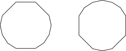
Figure 1: Mallows and Clark’s counter-example

whereas Waksman [W] pointed out that it is exceptional by showing that a “generic” planar convex polygon can be identified by the chord length distribution.

On the other hand, for general case, Caelli [Ca] gave a method to produce pairs of non-congruent subsets of $\mathbb{R}^{2}$, which are not convex in general, with the same interpoint distance distribution by using two axes of symmetry, as is illustrated in Figure 2.

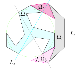
Figure 2: Let $I_{1}$ and $I_{2}$ be reflections in lines $L_{1}$ and $L_{2}$ respectively, which form the angle $q\pi$ $(q\in\mathbb{Q})$. Then $R=I_{1}I_{2}$ is the rotation by angle $2q\pi$. Let $\Omega_{1},\Omega_{2}$ and $\Omega_{3}$ be mutually disjoint regions satisfying $I_{1}\Omega_{1}=\Omega_{1}$, $I_{2}\Omega_{2}=\Omega_{2}$, $R\,\Omega_{3}=\Omega_{3}$ and $I_{1}\Omega_{3}\neq\Omega_{3}$. Then $X=\Omega_{1}\cup\Omega_{3}\cup\Omega_{2}$ and $X^{\prime}=\Omega_{1}\cup\Omega_{3}\cup R\,\Omega_{2}$ are not congruent, although they have the same interpoint distance distribution since $R\,\Omega_{2}=I_{1}\Omega_{2}$ implies $X^{\prime}=\Omega_{1}\cup R\,(\Omega_{3}\cup\Omega_{2})=\Omega_{3}\cup I_{1}(\Omega_{1}\cup\Omega_{2})$. This is a picture after Caelli’s paper.

Let us next consider a weaker problem, whether balls and spheres can be identified by the interpoint distance distribution. Again, the picutre is different according to whether we assume convexity or not.

Among convex bodies $K$, balls can be identified by the interpoint distance distribution. It follows directly from the fact that only balls give the maximum of the Riesz energy $I_{q}(K)$ for $-d<q<0$ among all convex bodies $K$ with a given volume $V=\sqrt{I_{0}(K)}$. This fact was proved by [D], [San1] and [Sch] independently. There is another proof. The volumes of a convex body $K$ and the boundary $\partial K$ can be expressed by the chord length distribution by

$$\int_{\mathcal{E}_{1}}L(K\cap\ell)\,d\mu(\ell)=\int_{0}^{\infty}rg_{K}^{\prime}(r)\,dr\quad\mbox{ and }\quad\int_{\mathcal{E}_{1}}\chi(K\cap\ell)\,d\mu(\ell)=\int_{0}^{\infty}g_{K}^{\prime}(r)\,dr$$

up to multiplication by constants, where $\chi$ is the Euler number. It is a consequence of Crofton’s intersection formula (see, for example [San2] 14.3 or [Fed] 3.2.26). Then the isoperimetric inequality in general dimension ([Fed]) implies the conclusion.

In this paper, we drop the assumption of convexity, and instead, we assume regularity of class $C^{3}$, namely, we restrict ouselves to the set of compact submanifolds $X$ of $\mathbb{R}^{d}$ of class $C^{3}$ with $\dim X=d$ or $\partial X=\emptyset$ ($\dim X<d$), and show that balls and circles can be identified by the beta function, and hence, by the interpoint distance distribution. We also show the identification of $2$-spheres under additional assumptions that the codimension of $X$ is not greater than $1$ and that the regularity is of class $C^{4}$.

2 Prelimanaries

We first show that the argument in [OS] goes almost parallel even if we weaken the assumption of regularity of $X$, and introduce some preceding results on the residues of the beta function from [B, FV, OS].

Let $M$ be an $m$ dimensional closed submanifold of $\mathbb{R}^{d}$ ($d>m$) and $x\in M$. Put

$$\psi_{M,x}(t)=\mbox{Vol}\left(M\cap B_{x}^{d}(t)\right)\,\mbox{ and }\>\varphi_{M,x}(t)=\psi_{M,x}^{\prime}(t),$$

where $B_{x}^{d}(t)$ is a $d$-ball with center $x$ and radius $t$. Then,

$$I_{z}(M)=\int_{M\times M}|x-y|^{z}\,dxdy=\int_{0}^{\infty}t^{z}\left(\int_{M}\varphi_{M,x}(t)\,dx\right)dt$$ (2.1)

for $\Re\mathfrak{e}\,z>-m$ ([OS] Proposition 3.3).

Let $\Omega$ be a compact body in $\mathbb{R}^{d}$ and $x\in M$. Put

$$\psi_{\nu,x}(t)=\int_{\partial\Omega\cap B_{x}^{d}(t)}\langle n_{x},n_{y}\rangle\,dy\>\mbox{ and }\>\varphi_{\nu,x}(t)=\psi_{\nu,x}^{\prime}(t),$$

where $n_{x}$ and $n_{y}$ are outer unit normal vectors to $\Omega$ at $x$ and $y$. Then,

$$\displaystyle I_{z}(\Omega)=\int_{\Omega\times\Omega}|x-y|^{z}\,dxdy = \displaystyle\frac{-1}{(z+2)(z+d)}\int_{\partial\Omega\times\partial\Omega}|x-y|^{z+2}\langle n_{x},n_{y}\rangle\,dxdy$$ (2.2)

$$= \displaystyle\frac{-1}{(z+2)(z+d)}\int_{0}^{\infty}t^{z+2}\left(\int_{\partial\Omega}\varphi_{\nu,x}(t)\,dx\right)dt$$ (2.3)

for $\Re\mathfrak{e}\,z>-d$ and $z\neq-2$ ([OS] Lemma 4.1).

Proposition 2.1

1. If $M$ is an $m$ dimensional closed submanifild of class $C^{k+1}$ $(k\geq 1)$, then

   $$\varphi_{M,x}(t)=t^{m-1}\,\overline{\varphi}_{M,x}(t)$$

   for some $\overline{\varphi}_{M,x}$ of class $C^{k}$. Moreover, $\overline{\varphi}_{M,x}(t)$ satisfies

   $$\overline{\varphi}_{M,x}(0)=\sigma_{m-1},\hskip 14.22636pt\frac{\partial^{2i-1}\,\overline{\varphi}_{M,x}}{\partial t^{2i-1}}(0)=0\>\>\>(1\leq 2i-1\leq k).$$

2. If $\Omega$ is a compact body of class $C^{k+1}$ $(k\geq 1)$, then $\varphi_{\nu,x}(t)=t^{d-2}\,\overline{\varphi}_{\nu,x}(t)$ for some $\overline{\varphi}_{\nu,x}$ of class $C^{k}$, which satisfies $\overline{\varphi}_{\nu,x}(0)=\sigma_{d-2}$ and $\overline{\varphi}_{\nu,x}^{(2i-1)}(0)=0$ $(1\leq 2i-1\leq k)$.

It is a $C^{k}$ analogue of Proposition 3.1 and Corollary 3.2 of [OS].

Proof. (1) Using the decomposition

$$\mathbb{R}^{d}\cong T_{x}\mathbb{R}^{d}=T_{x}M\oplus(T_{x}M)^{\perp}\cong\mathbb{R}^{m}\oplus\mathbb{R}^{d-m}$$

we can express a neighbourhood $N_{x}(M)$ of $x$ of $M$ as a graph of a function from $\mathbb{R}^{d}$ to $\mathbb{R}^{d-m}$. Let $S^{m-1}$ be the unit sphere in $T_{x}M\cong\mathbb{R}^{m}$. For a unit vector $v\in S^{m-1}$, let $s$ be the arc-length parameter of a curve $\gamma_{x,v}=N_{x}(M)\cap\left(\mbox{Span}\langle v\rangle\oplus\mathbb{R}^{d-m}\right)$ with $s=0$ at point $x$ and $\gamma_{x,v}^{\prime}(0)=v$. Let $t$ be another parameter of the curve given by the distance from the point $x$ endowed with the same signature as $s$. Then $s=s(x,v,t)$ is a function of $t$ of class $C^{k+1}$ defined on an open interval containing $0$. Then for small $t_{0}>0$,

$$\psi_{M,x}(t_{0})=\int_{0}^{t_{0}}\left(\int_{S^{m-1}}\frac{\partial s}{\partial t}(x,v,t)\,t^{m-1}\,dv\right)dt,$$

and therefore,

$$\varphi_{M,x}(t_{0})=t_{0}^{m-1}\int_{S^{m-1}}\frac{\partial s}{\partial t}(x,v,t_{0})\,dv,$$

which implies the first statement.

Since $({\partial t}/{\partial s})(0)=1$ we have $({\partial s}/{\partial t})(x,v,0)=1$, which implies $\overline{\varphi}_{M,x}(0)=\sigma_{m-1}$.

Since $s(x,v,t)=s(x,-v,-t)$ we have

$$\begin{array}[]{rcl}\overline{\varphi}_{M,x}(t_{0})&=&\displaystyle\int_{S^{m-1}}\frac{1}{2}\left(\frac{\partial s}{\partial t}(x,v,t_{0})+\frac{\partial s}{\partial t}(x,-v,t_{0})\right)dv\\[11.38109pt] &=&\displaystyle\int_{S^{m-1}}\frac{1}{2}\left(\frac{\partial s}{\partial t}(x,v,t_{0})+\frac{\partial s}{\partial t}(x,v,-t_{0})\right)dv,\end{array}$$

which implies $\overline{\varphi}_{M,x}^{(2i-1)}(0)=0$ $(1\leq 2i-1\leq k)$.

(2) The same statements for $\overline{\varphi}_{\nu,x}(t)$ can be proved in the same way. $\Box$

Since the formulae (2.1) and (2.3) imply

$$\begin{array}[]{l}\displaystyle I_{z}(M)=\int_{0}^{\infty}t^{z+m-1}\left(\int_{M}\overline{\varphi}_{M,x}(t)\,dx\right)dt,\\[11.38109pt] \displaystyle I_{z}(\Omega)=\frac{-1}{(z+2)(z+d)}\int_{0}^{\infty}t^{z+d}\left(\int_{\partial\Omega}\overline{\varphi}_{\nu,x}(t)\,dx\right)dt,\end{array}$$

the regularization of $I_{z}(M)$ and $I_{z}(\Omega)$ can be reduced to that of an integral of the form $I_{w,\phi}=\int_{0}^{\infty}t^{w}\phi(t)\,dt$. If $\phi(t)$ is of class $C^{k}$ then the integrand of the first term of the right hand side of

$$\begin{array}[]{rcl}\displaystyle I_{w,\phi}=\int_{0}^{\infty}t^{w}\,\phi(t)\,dt&=&\displaystyle\int_{0}^{1}t^{w}\left[\phi(t)-\phi(0)-\phi^{\prime}(0)t-\dots-\frac{\phi^{(k-1)}(0)}{(k-1)!}\,t^{k-1}\right]\,dt\\[14.22636pt] &&\displaystyle+\int_{1}^{\infty}t^{w}\,\phi(t)\,dt+\sum_{1\leq j\leq k}\frac{\phi^{(j-1)}(0)}{(j-1)!\,(z+j)}\end{array}$$

([GS] Ch.1, 3.2) can be estimated by $t^{w+k}$, and hence the integral converges for $\Re\mathfrak{e}\,w>-k-1$. Therefore $I_{w,\phi}=\int_{0}^{\infty}t^{w}\phi(t)\,dt$ is meromorphic on $\Re\mathfrak{e}\,w>-k-1$ having possible simple poles at $z=-1,\dots,-k$ with the residue at $z=-j$ given by $\phi^{(j-1)}/(j-1)!$ for $j=1,\dots,k$. Since $\overline{\varphi}_{M,x}$ and $\overline{\varphi}_{\nu,x}$ are of class $C^{k}$ and $\overline{\varphi}_{M,x}^{(2i-1)}(0)=\overline{\varphi}_{\nu,x}^{(2i-1)}(0)=0$, by putting $w=z+m-1$ for $M$ or $w=z+d$ for $\Omega$, we obtain the following.

Corollary 2.2

1. Suppose $M$ is an $m$ dimensional closed submanifold of $\mathbb{R}^{d}$ of class $C^{k+1}$ $(k\geq 1)$. The beta function $B_{M}(z)$ is meromorphic on $\Re\mathfrak{e}\,z>-m-k$ which has possible simple poles at $z=-m-2i$, where $0\leq 2i\leq k-1$, with

   $$\mbox{\rm Res}(B_{M},-m-2i)=\frac{1}{(2i)!}\int_{M}\overline{\varphi}_{M,x}^{(2i)}(0)\,dx\hskip 14.22636pt(0\leq 2i\leq k-1).$$

   In particular,

   $$\mbox{\rm Res}(B_{M},-m)=\sigma_{m-1}\mbox{\rm Vol}\,(M),$$ (2.4)

   where $\sigma_{j}$ is the volume of the unit $j$-sphere.

2. Suppose $\Omega$ is a compact body in $\mathbb{R}^{d}$ of class $C^{k+1}$ $(k\geq 1)$. The beta function $B_{\Omega}(z)$ is meromorphic on $\Re\mathfrak{e}\,z>-d-k-1$ which has possible simple poles at $z=-d$ and $z=-d-(2i+1)$, where $1\leq 2i+1\leq k$, with

   $$\mbox{\rm Res}(B_{\Omega},-d-(2i+1))=\frac{-1}{(d+2i-1)(2i+1)!}\int_{\partial\Omega}\overline{\varphi}_{\nu,x}^{(2i)}(0)\,dx\hskip 14.22636pt(1\leq 2i+1\leq k).$$

   In particular,

   $$\mbox{\rm Res}\,(B_{\Omega},-d-1)=-\frac{\sigma_{d-2}}{d-1}\mbox{\rm Vol}\,(\partial\Omega).$$ (2.5)

Remark 2.3

• The equation (2.4) for smooth closed curves was given in [B]. Two formulae of residues and the eqation (2.5) for smooth case were given in [OS].

• When $M$ is a closed surface in $\mathbb{R}^{3}$, the second residue which appears at $z=-4$ is given by

  $$\mbox{\rm Res}\,(B_{M},-4)=\frac{\pi}{8}\int_{M}(\kappa_{1}-\kappa_{2})^{2}dx,$$ (2.6)

  where $\kappa_{1}$ and $\kappa_{2}$ are principal curvatures of $M$ (Theorem 4.1 of [FV]; see also Proposition 3.8 of [OS] for the correction of the coefficient).

• The first residue of $B_{\Omega}(z)$ which appears at $z=-d$ is given by

  $$\mbox{\rm Res}\,(B_{\Omega},-d)=\sigma_{d-1}\mbox{\rm Vol}\,(\Omega),$$ (2.7)

  which can be computed using (2.2) without using differentiability of $\overline{\varphi}_{\nu,x}(t)$ ([OS] Lemma 4.5).

• The residues of the beta function do not indicate the number of the connected components of $X$ immediately.

3 Identification of balls and spheres

Let $B^{n}(r),S^{1}(r)$, and $S^{2}(r)$ be an $n$-ball, circle, and a $2$-sphere of radius $r$ respectively.

Lemma 3.1

If $X$ is a disjoint union of closed curves in $\mathbb{R}^{d}$, $B_{X}(-2)\geq 0$ with equality if and only if $X$ is a single circle.

Proof. Brylinski showed that $B_{C}(-2)=E(C)-4$ for a single curve $C$, where $E(C)$ is the so-called Möbius energy defined in [O] and studied in [FHW]. Freedman, He and Wang showed that $E(C)\geq 4$ for any single closed curve $C$ in $\mathbb{R}^{3}$ with equality if and only if $C$ is a circle. The easiest way to see this would be the “wasted length” argument and the cosine formula of $E$ by Doyle and Schramm (reported in [AS]).

Since the definition of the energy and the proofs of the above statements do not use the condition that the dimension of the ambiet space is equal to $3$, the above argument holds regardless of the codimension.

Suppose $X$ is a disjoint union of $n$ closed curves; $X=C_{1}\cup\dots\cup C_{n}$. We have

$$B_{X}(-2)=\sum_{i=1}^{n}B_{C_{i}}(-2)+2\sum_{i<j}\int_{C_{i}}\int_{C_{j}}|x-y|^{-2}\,dxdy\geq\sum_{i=1}^{n}B_{C_{i}}(-2)\geq 0,$$

where the second equality holds if and only if $C_{i}$ is a circle for any $i$ and the first equality holds if and only if $n=1$. $\Box$

Lemma 3.2

Let $X=S^{2}_{1}(r_{1})\cup S^{2}_{2}(r_{2})$ be a disjoint union of two $2$-spheres in $\mathbb{R}^{3}$ with radii $r_{1}$ and $r_{2}$ such that the diameter of $X$ is not greater than $2$. Put

$$\Delta_{2-\varepsilon}^{c}=\left\{(x,y)\in\mathbb{R}^{3}\times\mathbb{R}^{3}\,:\,|x-y|>2-\varepsilon\right\}.$$

Then there are positive constants $\varepsilon_{1}$ and $C$ such that if $0<\varepsilon<\varepsilon_{1}$ then

$$\frac{\mbox{\rm Vol}\left((S^{2}_{1}(r_{1})\times S^{2}_{2}(r_{2}))\cap\Delta_{2-\varepsilon}^{c}\right)}{\mbox{\rm Vol}\left(S^{2}_{1}(r_{1})\times S^{2}_{2}(r_{2})\right)}<C\varepsilon^{2}.$$

Proof. Put $\varepsilon_{1}=\min\{1,r_{1},r_{2}\}$. Since the numerator of the left hand side of (3.2) is an increasing function of the distance between two spheres, we have only to show the inequality when the distance is equal to $1-2r_{1}-2r_{2}$. Therefore we may assume both $S^{2}_{1}(r_{1})$ and $S^{2}_{2}(r_{2})$ are contained in the unit ball with center the origin.

If $(x,y)\in(S^{2}_{1}(r_{1})\times S^{2}_{2}(r_{2}))\cap\Delta_{2-\varepsilon}^{c}$ then

$$2-\varepsilon<|x-y|\leq|x|+|y|\leq|x|+1,$$

which means that $x$ is in the complement of the ball with center the origin and radius $1-\varepsilon$, which we denote by $\left(B^{3}(1-\varepsilon)\right)^{c}$. Since

$$A\left(S^{2}_{1}(r_{1})\cap\left(B^{3}(1-\varepsilon)\right)^{c}\,\right)=2\pi r_{1}\,\frac{\varepsilon(1-\frac{\varepsilon}{2})}{1-r_{1}},$$

where $A$ means the area. We have

$$\begin{array}[]{rcl}\displaystyle\frac{\mbox{Vol}\left((S^{2}_{1}(r_{1})\times S^{2}_{2}(r_{2}))\cap\Delta_{2-\varepsilon}^{c}\right)}{\mbox{Vol}\left(S^{2}_{1}(r_{1})\times S^{2}_{2}(r_{2})\right)}&\leq&\displaystyle\frac{A\left(S^{2}_{1}(r_{1})\cap\left(B^{3}(1-\varepsilon)\right)^{c}\,\right)\cdot A\left(S^{2}_{2}(r_{2})\cap\left(B^{3}(1-\varepsilon)\right)^{c}\,\right)}{A\left(S^{2}_{1}(r_{1})\right)\cdot A\left(S^{2}_{2}(r_{2})\right)}\\[11.38109pt] &=&\displaystyle\frac{\varepsilon^{2}(1-\frac{\varepsilon}{2})^{2}}{4r_{1}r_{2}(1-r_{1})(1-r_{2})},\end{array}$$

which implies that if we put

$$C=\frac{1}{4r_{1}r_{2}(1-r_{1})(1-r_{2})}$$

then the inequality (3.2) is satisfied. $\Box$

Lemma 3.3

Suppose $X$ is a disjoint union of $n$ two dimensional spheres in $\mathbb{R}^{3}$ that has the same area and diameter as $S^{2}(r)$. If $n>1$ then $X$ has a different interpoint distance distribution, and hence a different beta function, from $S^{2}(r)$.

Proof. We may assume without loss of generality that $r=1$. Assume that $X=S^{2}_{1}(r_{1})\cup\dots\cup S^{2}_{n}(r_{n})$ with $n>1$, $r_{1}\geq\dots\geq r_{n}$, $r_{1}^{2}+\cdots+r_{n}^{2}=1$ and that the diameter of $X$ is equal to $2$. Put $\varepsilon_{0}=\min\{2-2r_{1},r_{n},1\}$. Then if $0<\varepsilon<\varepsilon_{0}$ then $(S^{2}_{i}(r_{i})\times S^{2}_{i}(r_{i}))\cap\Delta_{2-\varepsilon}^{c}=\emptyset$ for any $i$. Therefore, Lemma 3.2 implies

$$\mbox{Vol}\left((X\times X)\cap\Delta_{2-\varepsilon}^{c}\right)\leq\sum_{i\neq j}\mbox{Vol}\left((S^{2}_{i}(r_{i})\times S^{2}_{j}(r_{j}))\cap\Delta_{2-\varepsilon}^{c}\right)\leq C_{0}\,\varepsilon^{2}\sum_{i\neq j}\mbox{Vol}\left(S^{2}_{i}(r_{i})\times S^{2}_{j}(r_{j})\right),$$

where

$$C_{0}=\max_{i\neq j}\frac{1}{4r_{i}r_{j}(1-r_{i})(1-r_{j})}.$$

If we take $\varepsilon>0$ so that $(C_{0}+\frac{1}{4})\varepsilon<1$ then

$$\mbox{Vol}\left((X\times X)\cap\Delta_{2-\varepsilon}^{c}\right)\leq C_{0}\,\varepsilon^{2}\,\mbox{Vol}\,(X\times X)<\left(\varepsilon-\frac{\varepsilon^{2}}{4}\right)\mbox{Vol}\,(S^{2}\times S^{2})=\mbox{Vol}\left((S^{2}\times S^{2})\cap\Delta_{2-\varepsilon}^{c}\right),$$

which completes the proof. $\Box$

Theorem 3.4

Assume $X$ is a compact submanifold of $\mathbb{R}^{d}$ that is either a body $(\dim X=d)$ or a closed submanifold $(\partial X=\emptyset,\,\dim X<d)$. Then the following hold up to congruence of $\mathbb{R}^{d}$.

1. If $X$ is a compact body of class $C^{2}$ and $B_{X}(z)=B_{B^{d}(r)}(z)$ holds for any $z\in\mathbb{C}$, then $X=B^{d}(r)$.

2. If $X$ is of class $C^{3}$ and $B_{X}(z)=B_{B^{n}(r)}(z)$ holds for any $z\in\mathbb{C}$, then $n=d$ and $X=B^{d}(r)$.

3. If $X$ is of class $C^{3}$ and $B_{X}(z)=B_{S^{1}(r)}(z)$ holds for any $z\in\mathbb{C}$, then $X=S^{1}(r)$.

4. If $X$ is of class $C^{4}$, $d-\dim X\leq 1$ and $B_{X}(z)=B_{S^{2}(r)}(z)$ for any $z\in\mathbb{C}$, then $d=3$ and $X=S^{2}(r)$.

Proof. We first give proof under the assumption that $X$ is smooth.

(1) By the equations (2.7) and (2.5), the residues at $z=-d$ and $-d-1$ imply that $\mbox{\rm Vol}(X)=\mbox{\rm Vol}(B^{d}(r))$ and $\mbox{\rm Vol}(\partial X)=\mbox{\rm Vol}(\partial B^{d}(r))$. Then the isoperimetric inequality in general dimension ([Fed]) implies that $X$ is an $d$-ball with radius $r$.

(2) Suppose $B_{X}(z)=B_{B^{n}}(z)$ for any $z\in\mathbb{C}$. The information of the poles implies that $X$ is a compact body in $\mathbb{R}^{n}$, and hence $n=d$ by the assumption of the theorem. The rest is same as in (1).

(3) Suppose $B_{X}(z)=B_{S^{1}}(z)$ for any $z\in\mathbb{C}$. The information of the poles implies that $X$ is a union of closed curves in $\mathbb{R}^{d}$. By Lemma 3.1, $X$ is a single circle. By the equation (2.4), the residue at $z=-1$ implies that $L(X)=2\pi r$, and hence $X=S^{1}(r)$.

(4) Suppose $B_{X}(z)=B_{S^{2}(r)}(z)$ for any $z\in\mathbb{C}$. The information of the poles implies that $X$ is a union of $2$-dimensional closed surfaces, and hence, by the additional assumption of the theorem, $d=3$. Since $\mbox{\rm Res}\,(B_{X},-4)=0$, the equation (2.6) shows that $X$ is totally umbilic, which implies that each connected component of $X$ is part of either a sphere or a plane (Meusnier 1785). Since $X$ is a closed surface, $X$ is a union of spheres. By (2.4), $\mbox{\rm Res}(B_{X},-2)=\mbox{\rm Res}(B_{S^{2}(r)},-2)$ implies that the area of $X$ is same as that of $S^{2}(r)$. Since the diameter of $X$ is given by $\lim_{n\to\infty}(B_{X}(n))^{1/n}$, $X$ has the same diameter as $S^{2}(r)$. Now the conclusion follows from Lemma 3.3.

We next show that the regularity of $X$ specified in each statement of the theorem is enough for the proof. Corollary 2.2 implies that if $M$ (or $\Omega$) is of class $C^{k+1}$, we obtain the first $k$ (or respectively, $k+1$) successive residues (including $0$) of $B_{M}(z)$ (or respectively, $B_{\Omega}(z)$) starting from $z=-m$ (or respectively, $z=-n$) which gives the first non-zero residue. Therefore, the regularity of $X$ guarantees the existence of a necessary number of residues for the proof of each statement. $\Box$

Corollary 3.5

Under the same assumption as in Theorem 3.4, balls, circles, and $2$-spheres can be identified by the interpoint distance distribution.

Jun O’Hara

Department of Mathematics and Informatics,Faculty of Science, Chiba University

1-33 Yayoi-cho, Inage, Chiba, 263-8522, JAPAN.

E-mail: ohara@math.s.chiba-u.ac.jp

References

• [AS] D.Β Auckly and L.Β Sadun, A family of MΓΆbius invariant 2-knot energies Geometric Topology (Proceedings of the 1993 Georgia International Topology Conference) AMS/IP Studies in Adv. Math., W. H. Kazez ed. Amer. Math. Soc. and International Press addr Cambridge, MA. (1997), 235 – 258
• [B] J.-L. Brylinski, The beta function of a knot. Internat. J. Math. 10 (1999), 415 – 423.
• [Ca] T.Β Caelli, On generating spatial configurations with identical interpoint distance distributions, in: Combinatorial Mathematics, VII (Proc. Seventh Australian Conf., Univ. Newcastle, Newcastle, 1979), in: Lecture Notes in Math., vol. 829, Springer, Berlin (1980), 69 – 75.
• [D] P.Β Davy, Inequalitiesf or moments of secant length, Z. Wahrscheinlichkeitsth 68 (1984), 243 – 246.
• [Fed] H.Β Federer, Geometric measure theory. Springer (1969).
• [Fen] W.Β Fenchel, Über KrΓΌmmung und Windung geschlossener Raumkurven. Math. Ann. 101 (1929), 238 – 252.
• [FHW] M. H.Β Freedman, Z-X.Β He and Z.Β Wang, MΓΆbius energy of knots and unknots. Ann. of Math. 139 (1994), 1 – 50.
• [FV] E. J.Β Fuller and M.K.Β Vemuri. The Brylinski Beta Function of a Surface. Geometriae Dedicata 179 (2015), 153 – 160, doi:10.1007/s10711-015-0071-y.
• [G] R.J.Gardner, Geometric Tomography, second edition, Cambridge University Press, New York, 2006.
• [GS] I.M. Gel’fand and G.E. Shilov, Generalized Functions. Volume I: Properties and Operations, Academic Press, New York and London, 1967.
• [MC] C.Β L.Β Mallows and J.Β M.Β C.Β Clark, Linear-Intercept Distributions Do Not Characterize Plane Sets. J. Appl. Prob. 7 (1970), 240 – 244.
• [M] B.Β MatΓ©rn, Spatial variation, Springer-Verlag, Berlin (1985).
• [O] J.Β O’Hara, Energy of a knot. Topology 30 (1991), 241 – 247.
• [OS] J.Β O’Hara and G.Β Solanes, Regularized Riesz energies of submanifolds. preprint, arXiv:1512.07935.
• [San1] L.A.Β SantalΓ³, On the measure of line segments entirely contained in a convex body, In Aspects of Mathematicsa nd Its Applications (North-Holland. Math. Library 34), North-Holland, Amsterdam (1986), 677 – 687.
• [San2] L.A.Β SantalΓ³, Integral Geometry and Geometric Probability, Addison- Wesley Publishing Company, 1976.
• [Sch] R.Β Schneider, Inequalitiesf or random flats meeting a convex body, J. Appl. Prob. 22 (1985), 710 – 716.
• [W] P.Β Waksman, Polygons and a conjecture of Blaschke’s, Adv. Appl. Prob. 17 (1985), 774 – 793.