Robust Wald-type tests for non-homogeneous observations based on minimum density power divergence estimator

Ayanendranath Basu1∗, Abhik Ghosh1, Nirian Martin2 and Leandro Pardo2
1 Indian Statistical Institute, Kolkata, India
2 Complutense University, Madrid, Spain
Corresponding author; Email: ayanbasu@isical.ac.in
Abstract

This paper considers the problem of robust hypothesis testing under non-identically distributed data. We propose Wald-type tests for both simple and composite hypothesis for independent but non-homogeneous observations based on the robust minimum density power divergence estimator of the common underlying parameter. Asymptotic and theoretical robustness properties of the proposed tests have been discussed. Application to the problem of testing the general linear hypothesis in a generalized linear model with fixed-design has been considered in detail with specific illustrations for its special cases under normal and Poisson distributions.

Keywords: Non-homogeneous Data; Robust Hypothesis Testing; Wald-Type Test; Minimum Density Power Divergence Estimator; Power Influence Function; Linear Regression; Poisson Regression.

1 Introduction

Suppose that the parametric model for the sample Y1,,Ynsubscript𝑌1subscript𝑌𝑛Y_{1},...,Y_{n} asserts that the distribution of Yisubscript𝑌𝑖Y_{i} is Fi,𝜽subscript𝐹𝑖𝜽F_{i,\boldsymbol{\theta}}, 𝜽Θ𝜽Θ\boldsymbol{\theta}\in\Theta pabsentsuperscript𝑝\subset\mathbb{R}^{p}. We shall denote by fi,𝜽subscript𝑓𝑖𝜽f_{i,\boldsymbol{\theta}} the probability density function associated with Fi,𝜽subscript𝐹𝑖𝜽F_{i,\boldsymbol{\theta}} with respect to a convenient σ𝜎\sigma-finite measure, for i=1,,n𝑖1𝑛i=1,...,n. This situation is very common for statistical modeling in many applications and an important example is the generalized linear model (GLM) with fixed design set-up.

The maximum likelihood score equation for these independently and non identically distributed data, Y1,,Ynsubscript𝑌1subscript𝑌𝑛Y_{1},...,Y_{n}, is given by

i=1n𝒖i,𝜽(yi)=𝟎,superscriptsubscript𝑖1𝑛subscript𝒖𝑖𝜽subscript𝑦𝑖0{\displaystyle\sum\limits_{i=1}^{n}}\boldsymbol{u}_{i,\boldsymbol{\theta}}\left(y_{i}\right)=\boldsymbol{0}, (1)

with 𝒖i,𝜽(yi)=𝜽logfi,𝜽(yi)subscript𝒖𝑖𝜽subscript𝑦𝑖𝜽subscript𝑓𝑖𝜽subscript𝑦𝑖\boldsymbol{u}_{i,\boldsymbol{\theta}}\left(y_{i}\right)=\frac{\partial}{\partial\boldsymbol{\theta}}\log f_{i,\boldsymbol{\theta}}(y_{i}). It is well-known that the maximum likelihood estimator, 𝜽^^𝜽\widehat{\boldsymbol{\theta}}, obtained as the solution of the system of equation (1), has serious problems of robustness. For this reason statistical solutions for several special cases like linear regression with normal errors (Huber, 1983; Muller, 1998) as well as some general cases (Beran, 1982; Ghosh and Basu, 2013) have been considered in the literature. In this paper, we shall follow the approach presented by Ghosh and Basu (2013) in order to propose some robust Wald-type tests. In the cited approach given by Ghosh and Basu (2013) a robust estimator was introduced based on the density power divergence (DPD) measure; details about this family of divergence measures can be found in Basu et al. (1998, 2011). This estimator, called the minimum density power divergence estimator (MDPDE) for non-homogeneous observations, is obtained as the solution of the system of equations

i=1n(fi,𝜽τ(Yi)𝒖i,𝜽(Yi)fi,𝜽τ+1(y)𝒖i,𝜽(y)𝑑y)=𝟎, τ>0.formulae-sequencesuperscriptsubscript𝑖1𝑛superscriptsubscript𝑓𝑖𝜽𝜏subscript𝑌𝑖subscript𝒖𝑖𝜽subscript𝑌𝑖superscriptsubscript𝑓𝑖𝜽𝜏1𝑦subscript𝒖𝑖𝜽𝑦differential-d𝑦0 𝜏0{\displaystyle\sum\limits_{i=1}^{n}}\left(f_{i,\boldsymbol{\theta}}^{\tau}(Y_{i})\boldsymbol{u}_{i,\boldsymbol{\theta}}\left(Y_{i}\right)-{\displaystyle\int}f_{i,\boldsymbol{\theta}}^{\tau+1}(y)\boldsymbol{u}_{i,\boldsymbol{\theta}}\left(y\right)dy\right)=\boldsymbol{0},\text{ }\tau>0. (2)

Note that in the limit as τ0𝜏0\tau\rightarrow 0, the system of equations given in (2) tends to the system given in (1).

In Ghosh and Basu (2013) it was established under some standard regularity conditions, that the asymptotic distribution of the MDPDE for non-homogeneous observations, say 𝜽^τsubscript^𝜽𝜏\widehat{\boldsymbol{\theta}}_{\tau}, at the true model distribution {fi,𝜽0:i=1,,n},conditional-setsubscript𝑓𝑖subscript𝜽0𝑖1𝑛\{f_{i,\boldsymbol{\theta}_{0}}:i=1,\ldots,n\}, is given by

𝛀n,τ1/2(𝜽0)𝚿n,τ(𝜽0)[n(𝜽^τ𝜽0)]n𝒩(𝟎,𝑰p),superscriptsubscript𝛀𝑛𝜏12subscript𝜽0subscript𝚿𝑛𝜏subscript𝜽0delimited-[]𝑛subscript^𝜽𝜏subscript𝜽0𝑛𝒩0subscript𝑰𝑝\boldsymbol{\Omega}_{n,\tau}^{-1/2}(\boldsymbol{\theta}_{0})\boldsymbol{\Psi}_{n,\tau}(\boldsymbol{\theta}_{0})\left[\sqrt{n}(\widehat{\boldsymbol{\theta}}_{\tau}-\boldsymbol{\theta}_{0})\right]\overset{\mathcal{L}}{\underset{n\mathcal{\rightarrow}\infty}{\longrightarrow}}\mathcal{N}\left(\boldsymbol{0},\boldsymbol{I}_{p}\right), (3)

or equivalently,

n(𝜽^τ𝜽0)n𝒩(𝟎,𝚺τ(𝜽0)),𝑛subscript^𝜽𝜏subscript𝜽0𝑛𝒩0subscript𝚺𝜏subscript𝜽0\sqrt{n}(\widehat{\boldsymbol{\theta}}_{\tau}-\boldsymbol{\theta}_{0})\overset{\mathcal{L}}{\underset{n\mathcal{\rightarrow}\infty}{\longrightarrow}}\mathcal{N}\left(\boldsymbol{0},\boldsymbol{\Sigma}_{\tau}(\boldsymbol{\theta}_{0})\right), (4)

with

𝚺τ(𝜽0)=limn𝚿n,τ1(𝜽0)𝛀n,τ(𝜽0)𝚿n,τ1(𝜽0),subscript𝚺𝜏subscript𝜽0subscript𝑛superscriptsubscript𝚿𝑛𝜏1subscript𝜽0subscript𝛀𝑛𝜏subscript𝜽0superscriptsubscript𝚿𝑛𝜏1subscript𝜽0\boldsymbol{\Sigma}_{\tau}(\boldsymbol{\theta}_{0})=\lim_{n\rightarrow\infty}\boldsymbol{\Psi}_{n,\tau}^{-1}(\boldsymbol{\theta}_{0})\boldsymbol{\Omega}_{n,\tau}(\boldsymbol{\theta}_{0})\boldsymbol{\Psi}_{n,\tau}^{-1}(\boldsymbol{\theta}_{0}), (5)

where we define

𝚿n,τ(𝜽)subscript𝚿𝑛𝜏𝜽\displaystyle\boldsymbol{\Psi}_{n,\tau}(\boldsymbol{\theta}) =1ni=1n𝑱i,τ(𝜽),absent1𝑛superscriptsubscript𝑖1𝑛subscript𝑱𝑖𝜏𝜽\displaystyle=\frac{1}{n}{\displaystyle\sum\limits_{i=1}^{n}}\boldsymbol{J}_{i,\tau}(\boldsymbol{\theta}), (6)
with 𝑱i,τ(𝜽)with subscript𝑱𝑖𝜏𝜽\displaystyle\mbox{with }~{}~{}~{}~{}~{}~{}~{}~{}~{}~{}~{}~{}~{}~{}~{}~{}~{}~{}~{}~{}~{}~{}~{}~{}~{}~{}~{}~{}~{}~{}\boldsymbol{J}_{i,\tau}(\boldsymbol{\theta}) =𝒖i,𝜽(y)𝒖i,𝜽T(y)fi,𝜽τ+1(y)𝑑y,absentsubscript𝒖𝑖𝜽𝑦superscriptsubscript𝒖𝑖𝜽𝑇𝑦superscriptsubscript𝑓𝑖𝜽𝜏1𝑦differential-d𝑦\displaystyle={\displaystyle\int}\boldsymbol{u}_{i,\boldsymbol{\theta}}\left(y\right)\boldsymbol{u}_{i,\boldsymbol{\theta}}^{T}\left(y\right)f_{i,\boldsymbol{\theta}}^{\tau+1}(y)dy,~{}~{}~{}~{}~{}~{}~{}~{}~{}~{}~{}~{}~{}~{}~{}~{}~{}~{}~{}~{}~{}~{}~{}~{}~{}~{}~{}~{}~{}~{}~{}~{}~{}~{}~{}~{}~{}~{}~{}~{}~{}~{}~{}~{}~{}~{}~{}~{}~{}~{}~{}~{}~{}~{}~{}~{}~{}~{}~{}~{}~{}~{}~{}~{}

and

𝛀n,τ(𝜽)subscript𝛀𝑛𝜏𝜽\displaystyle\boldsymbol{\Omega}_{n,\tau}(\boldsymbol{\theta}) =1ni=1n(𝒖i,𝜽(y)𝒖i,𝜽T(y)fi,𝜽2τ+1(yi)𝑑y𝝃i,τ(𝜽)𝝃i,τT(𝜽)),absent1𝑛superscriptsubscript𝑖1𝑛subscript𝒖𝑖𝜽𝑦superscriptsubscript𝒖𝑖𝜽𝑇𝑦superscriptsubscript𝑓𝑖𝜽2𝜏1subscript𝑦𝑖differential-d𝑦subscript𝝃𝑖𝜏𝜽superscriptsubscript𝝃𝑖𝜏𝑇𝜽\displaystyle=\frac{1}{n}{\displaystyle\sum\limits_{i=1}^{n}}\left({\displaystyle\int}\boldsymbol{u}_{i,\boldsymbol{\theta}}\left(y\right)\boldsymbol{u}_{i,\boldsymbol{\theta}}^{T}\left(y\right)f_{i,\boldsymbol{\theta}}^{2\tau+1}(y_{i})dy-\boldsymbol{\xi}_{i,\tau}(\boldsymbol{\theta})\boldsymbol{\xi}_{i,\tau}^{T}(\boldsymbol{\theta})\right),~{}~{}~{}~{}~{}~{}~{}~{}~{}~{}~{}~{}~{}~{}~{}~{}~{}~{}~{} (7)
with 𝝃i,τ(𝜽)with subscript𝝃𝑖𝜏𝜽\displaystyle\mbox{with }~{}~{}~{}~{}~{}~{}~{}~{}~{}~{}~{}~{}~{}~{}~{}~{}~{}~{}~{}~{}~{}~{}~{}~{}~{}~{}\boldsymbol{\xi}_{i,\tau}(\boldsymbol{\theta}) =𝒖i,𝜽(y)fi,𝜽τ(y)𝑑y.absentsubscript𝒖𝑖𝜽𝑦superscriptsubscript𝑓𝑖𝜽𝜏𝑦differential-d𝑦\displaystyle={\displaystyle\int}\boldsymbol{u}_{i,\boldsymbol{\theta}}\left(y\right)f_{i,\boldsymbol{\theta}}^{\tau}(y)dy. (8)

The required regularity conditions are listed in Appendix A for the sake of completeness and will be referred as the “Ghosh-Basu Conditions” throughout the rest of the paper.

Motivated by the strong robustness properties of the Wald-type test statistics based on MDPDEs (Basu et al., 2016, 2017a; Ghosh et al., 2016, 2017) in case of independently and identically distributed observations, in this paper we shall introduce and study the corresponding MDPDE based Wald-type tests for independently but non identically distributed data. In particular, we will develop the asymptotic and theoretical robustness of these Wald-type tests for both simple and composite hypotheses, along with applications to the generalized linear models (GLMs) and its important subclasses. It is important to note that there is no established robust hypothesis testing procedure under such general non-homogeneous data set-up except for one recent attempt by Ghosh and Basu (2017), who developed the divergence based test statistics with DPD measure. However, the asymptotic null distribution of their proposed test statistics is a linear combination of chi-square distributions occasionally limiting its application in complicated situations. On the contrary, our proposed Wald-type test statistics in this paper will be shown to have an ordinary chi-square distribution along with all the other competitive properties and hence easier to implement in any practical applications.

The rest of the paper is organized as follows: In Section 2, we shall introduce the Wald-type tests for testing simple null hypothesis as well as composite null hypothesis and we study their asymptotic distributions under the null hypotheses as well as alternative hypotheses. The robustness of these Wald-type tests will be studied in Section 3. In Section 4 the results are particularized to the GLM model. Some examples are studied in Section 5 and the paper ends with some insightful discussions in Section 6.

2 Wald-type tests under independent but non-homogeneous data

In the following two sections we shall consider the simple null hypothesis as well as composite null hypothesis versions of the Wald-type test statistics for independently and non identically distributed data.

2.1 Wald-type tests for simple null hypotheses

Let Y1,,Ynsubscript𝑌1subscript𝑌𝑛Y_{1},...,Y_{n} independently and non identically distributed data according to the probability density function fi,𝜽subscript𝑓𝑖𝜽f_{i,\boldsymbol{\theta}}, where 𝜽Θp.𝜽Θsuperscript𝑝\boldsymbol{\theta}\in\Theta\subset\mathbb{R}^{p}. In this section we define a family of Wald-type test statistics based on MDPDE for testing the hypothesis

H0:𝜽=𝜽0 against H1:𝜽𝜽0,:subscript𝐻0𝜽subscript𝜽0 against subscript𝐻1:𝜽subscript𝜽0H_{0}:\boldsymbol{\theta}=\boldsymbol{\theta}_{0}\text{ against }H_{1}:\boldsymbol{\theta}\neq\boldsymbol{\theta}_{0}, (9)

for a given 𝜽0Θsubscript𝜽0Θ\boldsymbol{\theta}_{0}\in\Theta, which will henceforth be referred to as the proposed Wald-type statistics.

Definition 1

Let 𝛉^τsubscript^𝛉𝜏\widehat{\boldsymbol{\theta}}_{\tau} be the MDPDE of 𝛉𝛉\boldsymbol{\theta}. The family of proposed Wald-type test statistics for testing the null hypothesis (9) is given by

Wn0(𝜽0)=n(𝜽^τ𝜽0)T𝚺τ1(𝜽0)(𝜽^τ𝜽0),superscriptsubscript𝑊𝑛0subscript𝜽0𝑛superscriptsubscript^𝜽𝜏subscript𝜽0𝑇superscriptsubscript𝚺𝜏1subscript𝜽0subscript^𝜽𝜏subscript𝜽0W_{n}^{0}(\boldsymbol{\theta}_{0})=n(\widehat{\boldsymbol{\theta}}_{\tau}-\boldsymbol{\theta}_{0})^{T}\boldsymbol{\Sigma}_{\tau}^{-1}(\boldsymbol{\theta}_{0})(\widehat{\boldsymbol{\theta}}_{\tau}-\boldsymbol{\theta}_{0}), (10)

where 𝚺τ(𝛉0)subscript𝚺𝜏subscript𝛉0\boldsymbol{\Sigma}_{\tau}(\boldsymbol{\theta}_{0}) is as defined in (5).

The asymptotic distribution of Wn0(𝜽0)superscriptsubscript𝑊𝑛0subscript𝜽0W_{n}^{0}(\boldsymbol{\theta}_{0}) is presented in the next theorem. The result follows easily from the asymptotic distribution of the MDPDE considered in (4) and so we omit the proof. Throughout the rest of the paper, for all the theoretical results, we will assume that the Ghosh-Basu conditions hold and 𝚺τ(𝜽)subscript𝚺𝜏𝜽\boldsymbol{\Sigma}_{\tau}(\boldsymbol{\theta}) is continuous in 𝜽Θ𝜽Θ\boldsymbol{\theta}\in\Theta.

Theorem 2

The asymptotic distribution, under the null hypothesis considered in (9), of the proposed Wald-type test statistics given in (10) is χp2superscriptsubscript𝜒𝑝2\chi_{p}^{2}, a chi-square distribution with p𝑝p degrees of freedom.

In the next Theorem we are going to present a result that will be important in order to get an approximation to the power function of the proposed Wald-type test statistic given in (10) because in many practical situation is not possible to get a simple expression for the exact power function.

Theorem 3

Let 𝛉superscript𝛉\boldsymbol{\theta}^{\ast} be the the true value of parameter with 𝛉𝛉0superscript𝛉subscript𝛉0\boldsymbol{\theta}^{\ast}\neq\boldsymbol{\theta}_{0}. Then, we have

n(s(𝜽^τ)s(𝜽))n𝒩(0,σWn0(𝜽0)2(𝜽))),\sqrt{n}(s(\widehat{\boldsymbol{\theta}}_{\tau})-s(\boldsymbol{\theta}^{\ast}))\overset{\mathcal{L}}{\underset{n\mathcal{\rightarrow}\infty}{\longrightarrow}}\mathcal{N}\left(0,\sigma_{W_{n}^{0}(\boldsymbol{\theta}_{0})}^{2}(\boldsymbol{\theta}^{\ast}))\right),

where s(𝛉)=(𝛉𝛉0)T𝚺τ1(𝛉0)(𝛉𝛉0)𝑠𝛉superscript𝛉subscript𝛉0𝑇superscriptsubscript𝚺𝜏1subscript𝛉0𝛉subscript𝛉0s\left(\boldsymbol{\theta}\right)=\left(\boldsymbol{\theta}-\boldsymbol{\theta}_{0}\right)^{T}\boldsymbol{\Sigma}_{\tau}^{-1}(\boldsymbol{\theta}_{0})\left(\boldsymbol{\theta}-\boldsymbol{\theta}_{0}\right) and σWn0(𝛉0)2(𝛉)=4(𝛉𝛉0)T[𝚺τ1(𝛉0)𝚺τ(𝛉)𝚺τ1(𝛉0)](𝛉𝛉0).superscriptsubscript𝜎superscriptsubscript𝑊𝑛0subscript𝛉02superscript𝛉4superscriptsuperscript𝛉subscript𝛉0𝑇delimited-[]superscriptsubscript𝚺𝜏1subscript𝛉0subscript𝚺𝜏superscript𝛉superscriptsubscript𝚺𝜏1subscript𝛉0superscript𝛉subscript𝛉0\sigma_{W_{n}^{0}(\boldsymbol{\theta}_{0})}^{2}(\boldsymbol{\theta}^{\ast})=4\left(\boldsymbol{\theta}^{\ast}-\boldsymbol{\theta}_{0}\right)^{T}\left[\boldsymbol{\Sigma}_{\tau}^{-1}(\boldsymbol{\theta}_{0})\boldsymbol{\Sigma}_{\tau}(\boldsymbol{\theta}^{\ast})\boldsymbol{\Sigma}_{\tau}^{-1}(\boldsymbol{\theta}_{0})\right]\left(\boldsymbol{\theta}^{\ast}-\boldsymbol{\theta}_{0}\right).

Proof. A first-order Taylor expansion of s(𝜽)𝑠𝜽s\left(\boldsymbol{\theta}\right) around 𝜽superscript𝜽\boldsymbol{\theta}^{\ast} at 𝜽^τsubscript^𝜽𝜏\widehat{\boldsymbol{\theta}}_{\tau} is given by

s(𝜽^τ)s(𝜽)=s(𝜽)𝜽T|𝜽=𝜽(𝜽^τ𝜽)+op(n1/2).𝑠subscript^𝜽𝜏𝑠superscript𝜽evaluated-at𝑠𝜽superscript𝜽𝑇𝜽superscript𝜽subscript^𝜽𝜏superscript𝜽subscript𝑜𝑝superscript𝑛12s(\widehat{\boldsymbol{\theta}}_{\tau})-s(\boldsymbol{\theta}^{\ast})=\left.\frac{\partial s\left(\boldsymbol{\theta}\right)}{\partial\boldsymbol{\theta}^{T}}\right|_{\boldsymbol{\theta=\theta}^{\ast}}(\widehat{\boldsymbol{\theta}}_{\tau}-\boldsymbol{\theta}^{\ast})+o_{p}(n^{-1/2}).

Then the asymptotic distribution of the random variable n(s(𝜽^τ)s(𝜽))𝑛𝑠subscript^𝜽𝜏𝑠superscript𝜽\sqrt{n}(s(\widehat{\boldsymbol{\theta}}_{\tau})-s(\boldsymbol{\theta}^{\ast})) matches the asymptotic distribution of the random variable s(𝜽)𝜽T|𝜽=𝜽n(𝜽^τ𝜽)evaluated-at𝑠𝜽superscript𝜽𝑇𝜽superscript𝜽𝑛subscript^𝜽𝜏superscript𝜽\left.\frac{\partial s\left(\boldsymbol{\theta}\right)}{\partial\boldsymbol{\theta}^{T}}\right|_{\boldsymbol{\theta=\theta}^{\ast}}\sqrt{n}\left(\widehat{\boldsymbol{\theta}}_{\tau}-\boldsymbol{\theta}^{\ast}\right) and the desired result follows.    

Based on Theorem 2 we shall reject the null hypothesis given in (9) if

Wn0(𝜽0)>χp,α2,superscriptsubscript𝑊𝑛0subscript𝜽0superscriptsubscript𝜒𝑝𝛼2W_{n}^{0}(\boldsymbol{\theta}_{0})>\chi_{p,\alpha}^{2}, (11)

and Theorem 3 makes it possible to have an approximation of the power function for the test given in (11). This is given by

πWn0(𝜽0)τ(𝜽)subscriptsuperscript𝜋𝜏superscriptsubscript𝑊𝑛0subscript𝜽0superscript𝜽\displaystyle\pi^{\tau}_{W_{n}^{0}(\boldsymbol{\theta}_{0})}(\boldsymbol{\theta}^{\ast}) =Pr(Rejecting H0|𝜽=𝜽)=Pr(Wn0(𝜽0)>χp,α2|𝜽=𝜽)absentPrconditionalRejecting subscript𝐻0𝜽superscript𝜽Prsuperscriptsubscript𝑊𝑛0subscript𝜽0conditionalsuperscriptsubscript𝜒𝑝𝛼2𝜽superscript𝜽\displaystyle=\Pr\left(\text{Rejecting }H_{0}|\boldsymbol{\theta}=\boldsymbol{\theta}^{\ast}\right)=\Pr\left(W_{n}^{0}(\boldsymbol{\theta}_{0})>\chi_{p,\alpha}^{2}|\boldsymbol{\theta}=\boldsymbol{\theta}^{\ast}\right)
=Pr(s(𝜽^τ)s(𝜽)>χp,α2ns(𝜽))absentPr𝑠subscript^𝜽𝜏𝑠superscript𝜽superscriptsubscript𝜒𝑝𝛼2𝑛𝑠superscript𝜽\displaystyle=\Pr\left(s(\widehat{\boldsymbol{\theta}}_{\tau})-s(\boldsymbol{\theta}^{\ast})>\frac{\chi_{p,\alpha}^{2}}{n}-s(\boldsymbol{\theta}^{\ast})\right)
=1Φn(n1/2σWn0(𝜽0)(𝜽)(χp,α2ns(𝜽))),absent1subscriptΦ𝑛superscript𝑛12subscript𝜎superscriptsubscript𝑊𝑛0subscript𝜽0superscript𝜽superscriptsubscript𝜒𝑝𝛼2𝑛𝑠superscript𝜽\displaystyle=1-\Phi_{n}\left(\frac{n^{1/2}}{\sigma_{W_{n}^{0}(\boldsymbol{\theta}_{0})}(\boldsymbol{\theta}^{\ast})}\left(\frac{\chi_{p,\alpha}^{2}}{n}-s(\boldsymbol{\theta}^{\ast})\right)\right), (12)

where χp,α2superscriptsubscript𝜒𝑝𝛼2\chi_{p,\alpha}^{2} denote the (1α)1𝛼(1-\alpha)-th quantile of χp2superscriptsubscript𝜒𝑝2\chi_{p}^{2} distribution, and Φn()subscriptΦ𝑛\Phi_{n}(\cdot) is a sequence of distribution functions tending uniformly to the standard normal distribution function Φ()Φ\Phi(\cdot). We can observe that the Wald-type tests are consistent in the Fraser sense since

limnπWn0(𝜽0)τ(𝜽)=1 τ0.subscript𝑛subscriptsuperscript𝜋𝜏superscriptsubscript𝑊𝑛0subscript𝜽0superscript𝜽1 for-all𝜏0\displaystyle\lim_{n\rightarrow\infty}\pi^{\tau}_{W_{n}^{0}(\boldsymbol{\theta}_{0})}(\boldsymbol{\theta}^{\ast})=1\text{ }\forall\tau\geq 0. (13)

This result can be applied in the sense of getting the necessary sample size for the Wald-type tests to have a predetermined power, πWn0(𝜽0)τ(𝜽)πsubscriptsuperscript𝜋𝜏superscriptsubscript𝑊𝑛0subscript𝜽0superscript𝜽superscript𝜋\pi^{\tau}_{W_{n}^{0}(\boldsymbol{\theta}_{0})}(\boldsymbol{\theta}^{\ast})\approx\pi^{\ast} and size α𝛼\alpha. The necessary sample size is given by

n=[A+B+A(A+2B)2s2(𝜽)]+1𝑛delimited-[]𝐴𝐵𝐴𝐴2𝐵2superscript𝑠2superscript𝜽1n=\left[\frac{A+B+\sqrt{A(A+2B)}}{2s^{2}(\boldsymbol{\theta}^{\ast})}\right]+1

where [z]delimited-[]𝑧\left[z\right] denotes the largest integer less than or equal to z𝑧z, A=σWn0(𝜽0)2(𝜽)(Φ1(1π))2,𝐴superscriptsubscript𝜎superscriptsubscript𝑊𝑛0subscript𝜽02superscript𝜽superscriptsuperscriptΦ11superscript𝜋2A=\sigma_{W_{n}^{0}(\boldsymbol{\theta}_{0})}^{2}(\boldsymbol{\theta}^{\ast})\left(\Phi^{-1}(1-\pi^{\ast})\right)^{2}, and B=2s(𝜽)χp,α2𝐵2𝑠superscript𝜽superscriptsubscript𝜒𝑝𝛼2B=2s(\boldsymbol{\theta}^{\ast})\chi_{p,\alpha}^{2}.

In order to produce a non-trivial asymptotic power, see (13), Cochran (1952) suggested using a set of local alternatives contiguous to the null hypothesis given in (9) as n𝑛n increases. In the next theorem we shall present the asymptotic distribution of the Wald-type test statistics under contiguous alternative hypotheses.

Theorem 4

Under the contiguous alternative hypothesis

H1,n:𝜽n=𝜽0+n1/2𝒅,:subscript𝐻1𝑛subscript𝜽𝑛subscript𝜽0superscript𝑛12𝒅H_{1,n}:\boldsymbol{\theta}_{n}=\boldsymbol{\theta}_{0}+n^{-1/2}\boldsymbol{d}, (14)

where 𝐝𝐝\boldsymbol{d} is a fixed vector in psuperscript𝑝\mathbb{R}^{p} such that 𝛉nΘpsubscript𝛉𝑛Θsuperscript𝑝\boldsymbol{\theta}_{n}\in\Theta\subset\mathbb{R}^{p}, the asymptotic distribution of the Wald-type test statistics given in (10) is χp2(δ)superscriptsubscript𝜒𝑝2𝛿\chi_{p}^{2}(\delta), a non-central chi-square distribution with p𝑝p degrees of freedom and non-centrality parameter

δ=𝒅T𝚺τ1(𝜽0)𝒅.𝛿superscript𝒅𝑇superscriptsubscript𝚺𝜏1subscript𝜽0𝒅\delta=\boldsymbol{d}^{T}\boldsymbol{\Sigma}_{\tau}^{-1}(\boldsymbol{\theta}_{0})\boldsymbol{d}. (15)

Proof. We can write

𝜽^τ𝜽0=𝜽^τ𝜽n+𝜽n𝜽0=(𝜽^τ𝜽n)+n1/2𝒅.subscript^𝜽𝜏subscript𝜽0subscript^𝜽𝜏subscript𝜽𝑛subscript𝜽𝑛subscript𝜽0subscript^𝜽𝜏subscript𝜽𝑛superscript𝑛12𝒅\widehat{\boldsymbol{\theta}}_{\tau}-\boldsymbol{\theta}_{0}=\widehat{\boldsymbol{\theta}}_{\tau}-\boldsymbol{\theta}_{n}+\boldsymbol{\theta}_{n}-\boldsymbol{\theta}_{0}=(\widehat{\boldsymbol{\theta}}_{\tau}-\boldsymbol{\theta}_{n})+n^{-1/2}\boldsymbol{d}.

Therefore, under H1,nsubscript𝐻1𝑛H_{1,n} given in (14), we have from (4),

n(𝜽^τ𝜽n)n𝒩(𝟎,𝚺τ(𝜽0))𝑛subscript^𝜽𝜏subscript𝜽𝑛𝑛𝒩0subscript𝚺𝜏subscript𝜽0\sqrt{n}(\widehat{\boldsymbol{\theta}}_{\tau}-\boldsymbol{\theta}_{n})\overset{\mathcal{L}}{\underset{n\mathcal{\rightarrow}\infty}{\longrightarrow}}\mathcal{N}\left(\boldsymbol{0},\boldsymbol{\Sigma}_{\tau}(\boldsymbol{\theta}_{0})\right)

and hence

n(𝜽^τ𝜽0)n𝒩(𝒅,𝚺τ(𝜽0)).𝑛subscript^𝜽𝜏subscript𝜽0𝑛𝒩𝒅subscript𝚺𝜏subscript𝜽0\sqrt{n}(\widehat{\boldsymbol{\theta}}_{\tau}-\boldsymbol{\theta}_{0})\overset{\mathcal{L}}{\underset{n\mathcal{\rightarrow}\infty}{\longrightarrow}}\mathcal{N}\left(\boldsymbol{d},\boldsymbol{\Sigma}_{\tau}(\boldsymbol{\theta}_{0})\right).

Note that Wn0(𝜽0)superscriptsubscript𝑊𝑛0subscript𝜽0W_{n}^{0}(\boldsymbol{\theta}_{0}) can be written by

Wn(𝜽0)=(n1/2𝚺τ1/2(𝜽0)(𝜽^τ𝜽0))T(n1/2𝚺τ1/2(𝜽0)(𝜽^τ𝜽0))subscript𝑊𝑛subscript𝜽0superscriptsuperscript𝑛12superscriptsubscript𝚺𝜏12subscript𝜽0subscript^𝜽𝜏subscript𝜽0𝑇superscript𝑛12superscriptsubscript𝚺𝜏12subscript𝜽0subscript^𝜽𝜏subscript𝜽0W_{n}(\boldsymbol{\theta}_{0})=\left(n^{1/2}\boldsymbol{\Sigma}_{\tau}^{-1/2}(\boldsymbol{\theta}_{0})(\widehat{\boldsymbol{\theta}}_{\tau}-\boldsymbol{\theta}_{0})\right)^{T}\left(n^{1/2}\boldsymbol{\Sigma}_{\tau}^{-1/2}(\boldsymbol{\theta}_{0})(\widehat{\boldsymbol{\theta}}_{\tau}-\boldsymbol{\theta}_{0})\right)

and under H1,nsubscript𝐻1𝑛H_{1,n} given in (14), we have,

n1/2𝚺τ1/2(𝜽0)(𝜽^τ𝜽0)n𝒩(𝚺τ1/2(𝜽0)𝒅,𝑰p×p).superscript𝑛12superscriptsubscript𝚺𝜏12subscript𝜽0subscript^𝜽𝜏subscript𝜽0𝑛𝒩superscriptsubscript𝚺𝜏12subscript𝜽0𝒅subscript𝑰𝑝𝑝n^{1/2}\boldsymbol{\Sigma}_{\tau}^{-1/2}(\boldsymbol{\theta}_{0})(\widehat{\boldsymbol{\theta}}_{\tau}-\boldsymbol{\theta}_{0})\overset{\mathcal{L}}{\underset{n\mathcal{\rightarrow}\infty}{\longrightarrow}}\mathcal{N}\left(\boldsymbol{\Sigma}_{\tau}^{-1/2}(\boldsymbol{\theta}_{0})\boldsymbol{d},\boldsymbol{I}_{p\times p}\right).

We apply the following result concerning quadratic forms. “If 𝒁𝒩(𝝁,𝚺)similar-to𝒁𝒩𝝁𝚺\boldsymbol{Z\sim}\mathcal{N}\left(\boldsymbol{\mu},\boldsymbol{\Sigma}\right), 𝚺𝚺\boldsymbol{\Sigma} is a symmetric projection of rank k𝑘k and 𝚺𝝁=𝝁𝚺𝝁𝝁\boldsymbol{\Sigma\mu=\mu}, then 𝒁T𝒁superscript𝒁𝑇𝒁\boldsymbol{Z}^{T}\boldsymbol{Z} is a chi-square distribution with k𝑘k degrees of freedom and non-centrality parameter 𝝁T𝝁superscript𝝁𝑇𝝁\boldsymbol{\mu}^{T}\boldsymbol{\mu}”. Therefore

Wn0(𝜽0)nχp2(δ),superscriptsubscript𝑊𝑛0subscript𝜽0𝑛superscriptsubscript𝜒𝑝2𝛿W_{n}^{0}(\boldsymbol{\theta}_{0})\overset{\mathcal{L}}{\underset{n\mathcal{\rightarrow}\infty}{\longrightarrow}}\chi_{p}^{2}\left(\delta\right),

where δ𝛿\delta was defined in (15).    

The last theorem permits us to get an approximation to the power function at 𝜽nsubscript𝜽𝑛\boldsymbol{\theta}_{n} by

πWn0(𝜽0)τ(𝜽n)=1Gχp2(δ)(χp,α2),subscriptsuperscript𝜋𝜏superscriptsubscript𝑊𝑛0subscript𝜽0subscript𝜽𝑛1subscript𝐺superscriptsubscript𝜒𝑝2𝛿superscriptsubscript𝜒𝑝𝛼2\displaystyle\pi^{\tau}_{W_{n}^{0}(\boldsymbol{\theta}_{0})}(\boldsymbol{\theta}_{n})=1-G_{\chi_{p}^{2}\left(\delta\right)}\left(\chi_{p,\alpha}^{2}\right), (16)

where Gχp2(δ)(z)subscript𝐺superscriptsubscript𝜒𝑝2𝛿𝑧G_{\chi_{p}^{2}\left(\delta\right)}\left(z\right) is the distribution function of χp2(δ)superscriptsubscript𝜒𝑝2𝛿\chi_{p}^{2}\left(\delta\right) evaluated at the point z𝑧z.

Based on this result we can also obtain an approximation of the power function at a generic point 𝜽superscript𝜽\boldsymbol{\theta}^{\ast}, because we can consider 𝒅=n1/2(𝜽𝜽0)𝒅superscript𝑛12superscript𝜽subscript𝜽0\boldsymbol{d}=n^{1/2}\left(\boldsymbol{\theta}^{\ast}-\boldsymbol{\theta}_{0}\right) and then 𝜽n=𝜽subscript𝜽𝑛superscript𝜽\boldsymbol{\theta}_{n}=\boldsymbol{\theta}^{\ast}.

2.2 Wald-type tests for composite null hypotheses

In many practical hypothesis testing problems, the restricted parameter space Θ0ΘsubscriptΘ0Θ\Theta_{0}\subset\Theta is defined by a set of r<p𝑟𝑝r<p non-redundant restrictions of the form

𝒉(𝜽)=𝟎𝒉𝜽0\boldsymbol{h}(\boldsymbol{\theta})=\boldsymbol{0} (17)

on ΘΘ\Theta, where 𝒉:pr:𝒉superscript𝑝superscript𝑟\boldsymbol{h}:\mathbb{R}^{p}\rightarrow\mathbb{R}^{r} is a vector-valued function such that the full rank p×r𝑝𝑟p\times r matrix

𝑯(𝜽)=𝒉(𝜽)𝜽T𝑯𝜽𝒉𝜽superscript𝜽𝑇\boldsymbol{H}\left(\boldsymbol{\theta}\right)=\frac{\partial\boldsymbol{h}(\boldsymbol{\theta})}{\partial\boldsymbol{\theta}^{T}} (18)

exists and is continuous in 𝜽𝜽\boldsymbol{\theta}.

Our interest will be in testing

H0:𝜽Θ0pr against H1:𝜽ΘΘ0:subscript𝐻0𝜽subscriptΘ0superscript𝑝𝑟 against subscript𝐻1:𝜽ΘsubscriptΘ0H_{0}:\boldsymbol{\theta}\in\Theta_{0}\subset{\mathbb{R}}^{p-r}\text{ against }H_{1}:\boldsymbol{\theta}\in\Theta-\Theta_{0} (19)

using Wald-type test statistics.

Definition 5

Let 𝛉^τsubscript^𝛉𝜏\widehat{\boldsymbol{\theta}}_{\tau} be the MDPDE of 𝛉𝛉\boldsymbol{\theta}. The family of proposed Wald-type test statistics for testing the composite null hypothesis (19) is given by

Wn(𝜽^τ)=n𝒉T(𝜽^τ)(𝑯T(𝜽^τ)𝚺τ(𝜽^τ)𝑯(𝜽^τ))1𝒉(𝜽^τ),subscript𝑊𝑛subscript^𝜽𝜏𝑛superscript𝒉𝑇subscript^𝜽𝜏superscriptsuperscript𝑯𝑇subscript^𝜽𝜏subscript𝚺𝜏subscript^𝜽𝜏𝑯subscript^𝜽𝜏1𝒉subscript^𝜽𝜏W_{n}(\widehat{\boldsymbol{\theta}}_{\tau})=n\boldsymbol{h}^{T}(\widehat{\boldsymbol{\theta}}_{\tau})\left(\boldsymbol{H}^{T}(\widehat{\boldsymbol{\theta}}_{\tau})\boldsymbol{\Sigma}_{\tau}(\widehat{\boldsymbol{\theta}}_{\tau})\boldsymbol{H}(\widehat{\boldsymbol{\theta}}_{\tau})\right)^{-1}\boldsymbol{h}(\widehat{\boldsymbol{\theta}}_{\tau}), (20)

In the next theorem we are going to present the asymptotic distribution of Wn(𝜽^τ)subscript𝑊𝑛subscript^𝜽𝜏W_{n}(\widehat{\boldsymbol{\theta}}_{\tau}).

Theorem 6

The asymptotic distribution of the Wald-type test statistics Wn(𝛉^τ)subscript𝑊𝑛subscript^𝛉𝜏W_{n}(\widehat{\boldsymbol{\theta}}_{\tau}), under the null hypothesis given in (19), is chi-squared with r𝑟r degrees of freedom.

Proof. Let 𝜽0Θ0subscript𝜽0subscriptΘ0\boldsymbol{\theta}_{0}\in\Theta_{0} be the true value of the parameter. A Taylor expansion gives

𝒉(𝜽^τ)𝒉subscript^𝜽𝜏\displaystyle\boldsymbol{h}(\widehat{\boldsymbol{\theta}}_{\tau}) =𝒉(𝜽0)+𝑯T(𝜽0)(𝜽^τ𝜽0)+op(n1/2𝟏)absent𝒉subscript𝜽0superscript𝑯𝑇subscript𝜽0subscript^𝜽𝜏subscript𝜽0subscript𝑜𝑝superscript𝑛121\displaystyle=\boldsymbol{h}(\boldsymbol{\theta}_{0})\boldsymbol{+H}^{T}(\boldsymbol{\theta}_{0})(\widehat{\boldsymbol{\theta}}_{\tau}-\boldsymbol{\theta}_{0})+o_{p}(n^{-1/2}\boldsymbol{1})
=𝑯T(𝜽0)(𝜽^τ𝜽0)+op(n1/2𝟏).absentsuperscript𝑯𝑇subscript𝜽0subscript^𝜽𝜏subscript𝜽0subscript𝑜𝑝superscript𝑛121\displaystyle=\boldsymbol{H}^{T}(\boldsymbol{\theta}_{0})(\widehat{\boldsymbol{\theta}}_{\tau}-\boldsymbol{\theta}_{0})+o_{p}(n^{-1/2}\boldsymbol{1}).

Under H0subscript𝐻0H_{0}

n(𝜽^τ𝜽0)n𝒩(𝟎p,𝚺τ(𝜽0))𝑛subscript^𝜽𝜏subscript𝜽0𝑛𝒩subscript0𝑝subscript𝚺𝜏subscript𝜽0\sqrt{n}(\widehat{\boldsymbol{\theta}}_{\tau}-\boldsymbol{\theta}_{0})\overset{\mathcal{L}}{\underset{n\mathcal{\rightarrow}\infty}{\longrightarrow}}\mathcal{N}\left(\boldsymbol{0}_{p},\boldsymbol{\Sigma}_{\tau}(\boldsymbol{\theta}_{0})\right)

and so

n𝒉(𝜽^τ)n𝒩(𝟎p,𝑯T(𝜽0)𝚺τ(𝜽0)𝑯(𝜽0)).𝑛𝒉subscript^𝜽𝜏𝑛𝒩subscript0𝑝superscript𝑯𝑇subscript𝜽0subscript𝚺𝜏subscript𝜽0𝑯subscript𝜽0\sqrt{n}\boldsymbol{h}(\widehat{\boldsymbol{\theta}}_{\tau})\overset{\mathcal{L}}{\underset{n\mathcal{\rightarrow}\infty}{\longrightarrow}}\mathcal{N}\left(\boldsymbol{0}_{p},\boldsymbol{H}^{T}(\boldsymbol{\theta}_{0})\boldsymbol{\Sigma}_{\tau}(\boldsymbol{\theta}_{0})\boldsymbol{H}(\boldsymbol{\theta}_{0})\right).

Taking into account that rank(𝑯(𝜽))=rrank𝑯𝜽𝑟\mathrm{rank}\left(\boldsymbol{H}\left(\boldsymbol{\theta}\right)\right)=r, we get

n𝒉T(𝜽^τ)(𝑯T(𝜽0)𝚺τ(𝜽0)𝑯(𝜽0))1𝒉(𝜽^τ)nχr2.𝑛superscript𝒉𝑇subscript^𝜽𝜏superscriptsuperscript𝑯𝑇subscript𝜽0subscript𝚺𝜏subscript𝜽0𝑯subscript𝜽01𝒉subscript^𝜽𝜏𝑛superscriptsubscript𝜒𝑟2n\boldsymbol{h}^{T}(\widehat{\boldsymbol{\theta}}_{\tau})\left(\boldsymbol{H}^{T}(\boldsymbol{\theta}_{0})\boldsymbol{\Sigma}_{\tau}(\boldsymbol{\theta}_{0})\boldsymbol{H}(\boldsymbol{\theta}_{0})\right)^{-1}\boldsymbol{h}(\widehat{\boldsymbol{\theta}}_{\tau})\overset{\mathcal{L}}{\underset{n\mathcal{\rightarrow}\infty}{\longrightarrow}}\chi_{r}^{2}.

But 𝑯T(𝜽^τ)𝚺τ(𝜽^τ)𝑯(𝜽^τ)superscript𝑯𝑇subscript^𝜽𝜏subscript𝚺𝜏subscript^𝜽𝜏𝑯subscript^𝜽𝜏\boldsymbol{H}^{T}(\widehat{\boldsymbol{\theta}}_{\tau})\boldsymbol{\Sigma}_{\tau}(\widehat{\boldsymbol{\theta}}_{\tau})\boldsymbol{H}(\widehat{\boldsymbol{\theta}}_{\tau}) is a consistent estimator of 𝑯T(𝜽0)𝚺τ(𝜽0)𝑯(𝜽0)superscript𝑯𝑇subscript𝜽0subscript𝚺𝜏subscript𝜽0𝑯subscript𝜽0\boldsymbol{H}^{T}(\boldsymbol{\theta}_{0})\boldsymbol{\Sigma}_{\tau}(\boldsymbol{\theta}_{0})\boldsymbol{H}(\boldsymbol{\theta}_{0}) by continuity of the matrices 𝑯(𝜽)𝑯𝜽\boldsymbol{H}(\boldsymbol{\theta}) and 𝚺τ(𝜽)subscript𝚺𝜏𝜽\boldsymbol{\Sigma}_{\tau}(\boldsymbol{\theta}) at 𝜽=𝜽0𝜽subscript𝜽0\boldsymbol{\theta}=\boldsymbol{\theta}_{0}. Then, it holds that

Wn(𝜽^τ)nχr2.subscript𝑊𝑛subscript^𝜽𝜏𝑛superscriptsubscript𝜒𝑟2W_{n}(\widehat{\boldsymbol{\theta}}_{\tau})\overset{\mathcal{L}}{\underset{n\mathcal{\rightarrow}\infty}{\longrightarrow}}\chi_{r}^{2}.


Based on the previous result, we shall reject the null hypothesis given in (19) if

Wn(𝜽^τ)>χr,α2.subscript𝑊𝑛subscript^𝜽𝜏superscriptsubscript𝜒𝑟𝛼2W_{n}(\widehat{\boldsymbol{\theta}}_{\tau})>\chi_{r,\alpha}^{2}. (21)

It is not easy to get an exact expression for the power function of the test given in (21). For that reason we are going to present a theorem that will be important in order to get an approximation of the power function for the test statistic presented in (21).

Theorem 7

Let 𝛉Θ0superscript𝛉subscriptΘ0\boldsymbol{\theta}^{\ast}\notin\Theta_{0} the true value of the parameter with 𝛉^τn𝒫𝛉subscript^𝛉𝜏𝒫𝑛superscript𝛉\widehat{\boldsymbol{\theta}}_{\tau}\overset{\mathcal{P}}{\underset{n\mathcal{\rightarrow}\infty}{\longrightarrow}}\boldsymbol{\theta}^{\ast}. Define

s(𝜽1,𝜽2)=𝒉T(𝜽1)(𝑯T(𝜽2)𝚺τ(𝜽2)𝑯(𝜽2))1𝒉(𝜽1).superscript𝑠subscript𝜽1subscript𝜽2superscript𝒉𝑇subscript𝜽1superscriptsuperscript𝑯𝑇subscript𝜽2subscript𝚺𝜏subscript𝜽2𝑯subscript𝜽21𝒉subscript𝜽1s^{\ast}\left(\boldsymbol{\theta}_{1},\boldsymbol{\theta}_{2}\right)=\boldsymbol{h}^{T}(\boldsymbol{\theta}_{1}\boldsymbol{)}\left(\boldsymbol{H}^{T}(\boldsymbol{\theta}_{2})\boldsymbol{\Sigma}_{\tau}(\boldsymbol{\theta}_{2})\boldsymbol{H}(\boldsymbol{\theta}_{2})\right)^{-1}\boldsymbol{h}(\boldsymbol{\theta}_{1}).

Then, we have

n(s(𝜽^τ,𝜽^τ)s(𝜽,𝜽))n𝒩(0,σ2(𝜽)),𝑛superscript𝑠subscript^𝜽𝜏subscript^𝜽𝜏superscript𝑠superscript𝜽superscript𝜽𝑛𝒩0superscript𝜎2superscript𝜽\sqrt{n}\left(s^{\ast}(\widehat{\boldsymbol{\theta}}_{\tau},\widehat{\boldsymbol{\theta}}_{\tau})-s^{\ast}(\boldsymbol{\theta}^{\ast},\boldsymbol{\theta}^{\ast})\right)\overset{\mathcal{L}}{\underset{n\mathcal{\rightarrow}\infty}{\longrightarrow}}\mathcal{N}\left(0,\sigma^{2}(\boldsymbol{\theta}^{\ast})\right),

where

σ2(𝜽)=4𝒉T(𝜽)(𝑯T(𝜽)𝚺τ(𝜽)𝑯(𝜽))1𝒉(𝜽).superscript𝜎2superscript𝜽4superscript𝒉𝑇superscript𝜽superscriptsuperscript𝑯𝑇superscript𝜽subscript𝚺𝜏superscript𝜽𝑯superscript𝜽1𝒉superscript𝜽\sigma^{2}(\boldsymbol{\theta}^{\ast})=4\boldsymbol{h}^{T}(\boldsymbol{\theta}^{\ast})\left(\boldsymbol{H}^{T}(\boldsymbol{\theta}^{\ast})\boldsymbol{\Sigma}_{\tau}(\boldsymbol{\theta}^{\ast})\boldsymbol{H}(\boldsymbol{\theta}^{\ast})\right)^{-1}\boldsymbol{h}(\boldsymbol{\theta}^{\ast}).

Proof. We can observe that s(𝜽^τ,𝜽^τ)superscript𝑠subscript^𝜽𝜏subscript^𝜽𝜏s^{\ast}(\widehat{\boldsymbol{\theta}}_{\tau},\widehat{\boldsymbol{\theta}}_{\tau}) and s(𝜽^τ,𝜽)superscript𝑠subscript^𝜽𝜏superscript𝜽s^{\ast}(\widehat{\boldsymbol{\theta}}_{\tau},\boldsymbol{\theta}^{\ast}) have the same asymptotic distribution because 𝜽^τn𝒫𝜽.subscript^𝜽𝜏𝒫𝑛superscript𝜽\widehat{\boldsymbol{\theta}}_{\tau}\overset{\mathcal{P}}{\underset{n\mathcal{\rightarrow}\infty}{\longrightarrow}}\boldsymbol{\theta}^{\ast}. A first-order Talyor expansion of s(𝜽,𝜽)superscript𝑠𝜽superscript𝜽s^{\ast}({\boldsymbol{\theta}},\boldsymbol{\theta}^{\ast}) at 𝜽^τsubscript^𝜽𝜏\widehat{\boldsymbol{\theta}}_{\tau} around 𝜽superscript𝜽\boldsymbol{\theta}^{\ast} gives

s(𝜽^τ,𝜽)s(𝜽,𝜽)=s(𝜽,𝜽)𝜽T|𝜽=𝜽(𝜽^τ𝜽)+op(n1/2).superscript𝑠subscript^𝜽𝜏superscript𝜽superscript𝑠superscript𝜽superscript𝜽evaluated-atsuperscript𝑠𝜽superscript𝜽superscript𝜽𝑇𝜽superscript𝜽subscript^𝜽𝜏superscript𝜽subscript𝑜𝑝superscript𝑛12s^{\ast}(\widehat{\boldsymbol{\theta}}_{\tau},\boldsymbol{\theta}^{\ast})-s^{\ast}(\boldsymbol{\theta}^{\ast},\boldsymbol{\theta}^{\ast})=\left.\frac{\partial s^{\ast}\left(\boldsymbol{\theta},\boldsymbol{\theta}^{\ast}\right)}{\partial\boldsymbol{\theta}^{T}}\right|_{\boldsymbol{\theta=\theta}^{\ast}}(\widehat{\boldsymbol{\theta}}_{\tau}-\boldsymbol{\theta}^{\ast})+o_{p}(n^{-1/2}).

Now the result follows, because

σ2(𝜽)=s(𝜽,𝜽)𝜽T|𝜽=𝜽𝚺τ(𝜽)s(𝜽,𝜽)𝜽|𝜽=𝜽.superscript𝜎2superscript𝜽evaluated-atevaluated-atsuperscript𝑠𝜽superscript𝜽superscript𝜽𝑇𝜽superscript𝜽subscript𝚺𝜏superscript𝜽superscript𝑠𝜽superscript𝜽𝜽𝜽superscript𝜽\sigma^{2}(\boldsymbol{\theta}^{\ast})=\left.\frac{\partial s^{\ast}\left(\boldsymbol{\theta},\boldsymbol{\theta}^{\ast}\right)}{\partial\boldsymbol{\theta}^{T}}\right|_{\boldsymbol{\theta=\theta}^{\ast}}\boldsymbol{\Sigma}_{\tau}(\boldsymbol{\theta}^{\ast})\left.\frac{\partial s^{\ast}\left(\boldsymbol{\theta},\boldsymbol{\theta}^{\ast}\right)}{\partial\boldsymbol{\theta}}\right|_{\boldsymbol{\theta=\theta}^{\ast}}.

and

s(𝜽,𝜽)𝜽T=2𝒉T(𝜽)(𝑯T(𝜽)𝚺τ(𝜽)𝑯(𝜽))1𝑯T(𝜽).superscript𝑠𝜽superscript𝜽superscript𝜽𝑇2superscript𝒉𝑇𝜽superscriptsuperscript𝑯𝑇superscript𝜽subscript𝚺𝜏superscript𝜽𝑯superscript𝜽1superscript𝑯𝑇𝜽\frac{\partial s^{\ast}\left(\boldsymbol{\theta},\boldsymbol{\theta}^{\ast}\right)}{\partial\boldsymbol{\theta}^{T}}=2\boldsymbol{h}^{T}(\boldsymbol{\theta})\left(\boldsymbol{H}^{T}(\boldsymbol{\theta}^{\ast})\boldsymbol{\Sigma}_{\tau}(\boldsymbol{\theta}^{\ast})\boldsymbol{H}(\boldsymbol{\theta}^{\ast})\right)^{-1}\boldsymbol{H}^{T}(\boldsymbol{\theta}).


Using the above theorem we can derive an approximation to the power of the proposed Wald-type tests of composite null hypothesis at any 𝜽Θ0superscript𝜽subscriptΘ0\boldsymbol{\theta}^{\ast}\notin\Theta_{0} using an argument similar to that of the derivation of the expression in (12) for the case of simple null hypothesis. This further indicates the consistency of our proposal at any fixed alternatives even for the composite hypotheses.

We may also find an approximation of the power of Wn(𝜽^τ)subscript𝑊𝑛subscript^𝜽𝜏W_{n}(\widehat{\boldsymbol{\theta}}_{\tau}) at an alternative close to the null hypothesis. Let 𝜽nΘΘ0subscript𝜽𝑛ΘsubscriptΘ0\boldsymbol{\theta}_{n}\in\Theta-\Theta_{0} be a given alternative and let 𝜽0subscript𝜽0\boldsymbol{\theta}_{0} be the element in Θ0subscriptΘ0\Theta_{0} closest to 𝜽nsubscript𝜽𝑛\boldsymbol{\theta}_{n} in the Euclidean distance sense. A first possibility to introduce contiguous alternative hypotheses is to consider a fixed 𝒅p𝒅superscript𝑝\boldsymbol{d}\in\mathbb{R}^{p} and to permit 𝜽nsubscript𝜽𝑛\boldsymbol{\theta}_{n} to move towards 𝜽0subscript𝜽0\boldsymbol{\theta}_{0} as n𝑛n increases through the relation

H1,n:𝜽n=𝜽0+n1/2𝒅.:subscript𝐻1𝑛subscript𝜽𝑛subscript𝜽0superscript𝑛12𝒅H_{1,n}:\boldsymbol{\theta}_{n}=\boldsymbol{\theta}_{0}+n^{-1/2}\boldsymbol{d}. (22)

A second approach is to relax the condition 𝒉(𝜽)=𝟎𝒉𝜽0\boldsymbol{h}\left(\boldsymbol{\theta}\right)=\boldsymbol{0} defining Θ0.subscriptΘ0\Theta_{0}. Let 𝒅rsuperscript𝒅superscript𝑟\boldsymbol{d}^{\ast}\in\mathbb{R}^{r} and consider the following sequence, {𝜽n}subscript𝜽𝑛\left\{\boldsymbol{\theta}_{n}\right\}, of parameters moving towards 𝜽0subscript𝜽0\boldsymbol{\theta}_{0} according to

H1,n:𝒉(𝜽n)=n1/2𝒅.:superscriptsubscript𝐻1𝑛𝒉subscript𝜽𝑛superscript𝑛12superscript𝒅H_{1,n}^{\ast}:\boldsymbol{h}(\boldsymbol{\theta}_{n})=n^{-1/2}\boldsymbol{d}^{\ast}. (23)

Note that a Taylor series expansion of 𝒉(𝜽n)𝒉subscript𝜽𝑛\boldsymbol{h}(\boldsymbol{\theta}_{n}) around 𝜽0subscript𝜽0\boldsymbol{\theta}_{0} yields

𝒉(𝜽n)=𝒉(𝜽0)+𝑯T(𝜽0)(𝜽n𝜽0)+o(𝜽n𝜽0𝟏).𝒉subscript𝜽𝑛𝒉subscript𝜽0superscript𝑯𝑇subscript𝜽0subscript𝜽𝑛subscript𝜽0𝑜normsubscript𝜽𝑛subscript𝜽01\displaystyle\boldsymbol{h}(\boldsymbol{\theta}_{n})=\boldsymbol{h}(\boldsymbol{\theta}_{0})+\boldsymbol{H}^{T}(\boldsymbol{\theta}_{0})\left(\boldsymbol{\theta}_{n}-\boldsymbol{\theta}_{0}\right)+o\left(\left\|\boldsymbol{\theta}_{n}-\boldsymbol{\theta}_{0}\right\|\boldsymbol{1}\right). (24)

By substituting 𝜽n=𝜽0+n1/2𝒅subscript𝜽𝑛subscript𝜽0superscript𝑛12𝒅\boldsymbol{\theta}_{n}=\boldsymbol{\theta}_{0}+n^{-1/2}\boldsymbol{d} in (24) and taking into account that h(θ0)=𝟎subscript𝜃00\boldsymbol{h}(\boldsymbol{\theta}_{0})=\boldsymbol{0}, we get

𝒉(𝜽n)=n1/2𝑯T(𝜽0)𝒅+o(𝜽n𝜽0𝟏),𝒉subscript𝜽𝑛superscript𝑛12superscript𝑯𝑇subscript𝜽0𝒅𝑜normsubscript𝜽𝑛subscript𝜽01\boldsymbol{h}(\boldsymbol{\theta}_{n})=n^{-1/2}\boldsymbol{H}^{T}(\boldsymbol{\theta}_{0})\boldsymbol{d}+o\left(\left\|\boldsymbol{\theta}_{n}-\boldsymbol{\theta}_{0}\right\|\boldsymbol{1}\right), (25)

so that the equivalence in the limit is obtained for 𝒅=𝑯T(𝜽0)𝒅superscript𝒅superscript𝑯𝑇subscript𝜽0𝒅\boldsymbol{d}^{\ast}\boldsymbol{=H}^{T}(\boldsymbol{\theta}_{0})\boldsymbol{d}.

Theorem 8

Under the contiguous alternative hypotheses given in (22) and (23), we have

  1. i)

    Wn(𝜽^τ)nχr2(a)subscript𝑊𝑛subscript^𝜽𝜏𝑛superscriptsubscript𝜒𝑟2𝑎W_{n}(\widehat{\boldsymbol{\theta}}_{\tau})\underset{n\rightarrow\infty}{\overset{\mathcal{L}}{\longrightarrow}}\chi_{r}^{2}\left(a\right) under H1,nsubscript𝐻1𝑛H_{1,n} given in (22), where the non-centrality parameter “a𝑎a” is given by

    a=𝒅T𝑯(𝜽0)(𝑯T(𝜽0)𝚺τ(𝜽0)𝑯(𝜽0))1𝑯T(𝜽0)𝒅.𝑎superscript𝒅𝑇𝑯subscript𝜽0superscriptsuperscript𝑯𝑇subscript𝜽0subscript𝚺𝜏subscript𝜽0𝑯subscript𝜽01superscript𝑯𝑇subscript𝜽0𝒅a=\boldsymbol{d}^{T}\boldsymbol{H}(\boldsymbol{\theta}_{0})\left(\boldsymbol{H}^{T}(\boldsymbol{\theta}_{0})\boldsymbol{\Sigma}_{\tau}(\boldsymbol{\theta}_{0})\boldsymbol{H}(\boldsymbol{\theta}_{0})\right)^{-1}\boldsymbol{H}^{T}(\boldsymbol{\theta}_{0})\boldsymbol{d}.
  2. ii)

    Wn(𝜽^τ)nχr2(b)subscript𝑊𝑛subscript^𝜽𝜏𝑛superscriptsubscript𝜒𝑟2𝑏W_{n}(\widehat{\boldsymbol{\theta}}_{\tau})\underset{n\rightarrow\infty}{\overset{\mathcal{L}}{\longrightarrow}}\chi_{r}^{2}\left(b\right) under H1,nsuperscriptsubscript𝐻1𝑛H_{1,n}^{\ast} given in (23), where the non-centrality parameter “b𝑏b” is given by

    b=𝒅T(𝑯T(𝜽0)𝚺τ(𝜽0)𝑯(𝜽0))1𝒅.𝑏superscript𝒅absent𝑇superscriptsuperscript𝑯𝑇subscript𝜽0subscript𝚺𝜏subscript𝜽0𝑯subscript𝜽01superscript𝒅b=\boldsymbol{\boldsymbol{d}}^{\ast T}\left(\boldsymbol{H}^{T}(\boldsymbol{\theta}_{0})\boldsymbol{\Sigma}_{\tau}(\boldsymbol{\theta}_{0})\boldsymbol{H}(\boldsymbol{\theta}_{0})\right)^{-1}\boldsymbol{\boldsymbol{d}}^{\ast}.

Proof. A Taylor series expansion of 𝒉(𝜽^τ)𝒉subscript^𝜽𝜏\boldsymbol{h}(\widehat{\boldsymbol{\theta}}_{{\tau}}) around 𝜽nsubscript𝜽𝑛\boldsymbol{\theta}_{n} yields

𝒉(𝜽^τ)=𝒉(𝜽n)+𝑯T(𝜽n)(𝜽^τ𝜽n)+o(𝜽^τ𝜽n𝟏).𝒉subscript^𝜽𝜏𝒉subscript𝜽𝑛superscript𝑯𝑇subscript𝜽𝑛subscript^𝜽𝜏subscript𝜽𝑛𝑜normsubscript^𝜽𝜏subscript𝜽𝑛1\boldsymbol{h}(\widehat{\boldsymbol{\theta}}_{{\tau}})=\boldsymbol{h}(\boldsymbol{\theta}_{n})+\boldsymbol{H}^{T}(\boldsymbol{\theta}_{n})(\widehat{\boldsymbol{\theta}}_{{\tau}}-\boldsymbol{\theta}_{n})+o\left(\left\|\widehat{\boldsymbol{\theta}}_{{\tau}}-\boldsymbol{\theta}_{n}\right\|\boldsymbol{1}\right).

From (25), we have

𝒉(𝜽^τ)=n1/2𝑯T(𝜽0)𝒅+𝑯T(𝜽n)(𝜽^τ𝜽n)+o(𝜽^τ𝜽n𝟏)+o(𝜽n𝜽0𝟏).𝒉subscript^𝜽𝜏superscript𝑛12superscript𝑯𝑇subscript𝜽0𝒅superscript𝑯𝑇subscript𝜽𝑛subscript^𝜽𝜏subscript𝜽𝑛𝑜normsubscript^𝜽𝜏subscript𝜽𝑛1𝑜normsubscript𝜽𝑛subscript𝜽01\boldsymbol{h}(\widehat{\boldsymbol{\theta}}_{{\tau}})=n^{-1/2}\boldsymbol{H}^{T}(\boldsymbol{\theta}_{0})\boldsymbol{d}+\boldsymbol{H}^{T}(\boldsymbol{\theta}_{n})(\widehat{\boldsymbol{\theta}}_{{\tau}}-\boldsymbol{\theta}_{n})+o\left(\left\|\widehat{\boldsymbol{\theta}}_{{\tau}}-\boldsymbol{\theta}_{n}\right\|\boldsymbol{1}\right)+o\left(\left\|\boldsymbol{\theta}_{n}-\boldsymbol{\theta}_{0}\right\|\boldsymbol{1}\right).

As n(𝜽^τ𝜽n)n𝒩(𝟎,𝚺τ(𝜽0))𝑛subscript^𝜽𝜏subscript𝜽𝑛𝑛𝒩0subscript𝚺𝜏subscript𝜽0\sqrt{n}(\widehat{\boldsymbol{\theta}}_{{\tau}}-\boldsymbol{\theta}_{n})\underset{n\rightarrow\infty}{\overset{\mathcal{L}}{\longrightarrow}}\mathcal{N}(\boldsymbol{0},\boldsymbol{\Sigma}_{\tau}(\boldsymbol{\theta}_{0})) and n(o(𝜽^τ𝜽n𝟏)+o(𝜽n𝜽0𝟏))=op(𝟏)𝑛𝑜normsubscript^𝜽𝜏subscript𝜽𝑛1𝑜normsubscript𝜽𝑛subscript𝜽01subscript𝑜𝑝1\sqrt{n}\left(o\left(\left\|\widehat{\boldsymbol{\theta}}_{{\tau}}-\boldsymbol{\theta}_{n}\right\|\boldsymbol{1}\right)+o\left(\left\|\boldsymbol{\theta}_{n}-\boldsymbol{\theta}_{0}\right\|\boldsymbol{1}\right)\right)=o_{p}\left(\boldsymbol{1}\right), we have

n𝒉(𝜽^τ)n𝒩(𝑯T(𝜽0)𝒅,𝑯T(𝜽0)𝚺τ(𝜽0)𝑯(𝜽0)).𝑛𝒉subscript^𝜽𝜏𝑛𝒩superscript𝑯𝑇subscript𝜽0𝒅superscript𝑯𝑇subscript𝜽0subscript𝚺𝜏subscript𝜽0𝑯subscript𝜽0\sqrt{n}\boldsymbol{h}(\widehat{\boldsymbol{\theta}}_{{\tau}})\underset{n\rightarrow\infty}{\overset{\mathcal{L}}{\longrightarrow}}\mathcal{N}(\boldsymbol{H}^{T}(\boldsymbol{\theta}_{0})\boldsymbol{d},\boldsymbol{H}^{T}(\boldsymbol{\theta}_{0})\boldsymbol{\Sigma}_{\tau}(\boldsymbol{\theta}_{0})\boldsymbol{H}(\boldsymbol{\theta}_{0})).

We can observe by the relationship 𝒅=𝑯T(𝜽0)𝒅superscript𝒅superscript𝑯𝑇subscript𝜽0𝒅\boldsymbol{d}^{\ast}\boldsymbol{=H}^{T}(\boldsymbol{\theta}_{0})\boldsymbol{d}, if 𝒉(𝜽n)=n1/2𝒅𝒉subscript𝜽𝑛superscript𝑛12superscript𝒅\boldsymbol{h}(\boldsymbol{\theta}_{n})=n^{-1/2}\boldsymbol{d}^{\ast} that

n𝒉(𝜽^τ)n𝒩(𝒅,𝑯T(𝜽0)𝚺τ(𝜽0)𝑯(𝜽0)).𝑛𝒉subscript^𝜽𝜏𝑛𝒩superscript𝒅superscript𝑯𝑇subscript𝜽0subscript𝚺𝜏subscript𝜽0𝑯subscript𝜽0\sqrt{n}\boldsymbol{h}(\widehat{\boldsymbol{\theta}}_{{\tau}})\underset{n\rightarrow\infty}{\overset{\mathcal{L}}{\longrightarrow}}\mathcal{N}(\boldsymbol{d}^{\ast},\boldsymbol{H}^{T}(\boldsymbol{\theta}_{0})\boldsymbol{\Sigma}_{\tau}(\boldsymbol{\theta}_{0})\boldsymbol{H}(\boldsymbol{\theta}_{0})).

In our case, the quadratic form is Wn=𝒁T𝒁subscript𝑊𝑛superscript𝒁𝑇𝒁W_{n}=\boldsymbol{Z}^{T}\boldsymbol{Z} with 𝒁=n𝒉(𝜽^τ)(𝑯T(𝜽0)𝚺τ(𝜽0)𝑯(𝜽0))1/2𝒁𝑛𝒉subscript^𝜽𝜏superscriptsuperscript𝑯𝑇subscript𝜽0subscript𝚺𝜏subscript𝜽0𝑯subscript𝜽012\boldsymbol{Z}=\sqrt{n}\boldsymbol{h}(\widehat{\boldsymbol{\theta}}_{{\tau}})\left(\boldsymbol{H}^{T}(\boldsymbol{\theta}_{0})\boldsymbol{\Sigma}_{\tau}(\boldsymbol{\theta}_{0})\boldsymbol{H}(\boldsymbol{\theta}_{0})\right)^{-1/2} and

𝒁n𝒩((𝑯T(𝜽0)𝚺τ(𝜽0)𝑯(𝜽0))1/2𝑯T(𝜽0)𝒅,𝑰),𝒁𝑛𝒩superscriptsuperscript𝑯𝑇subscript𝜽0subscript𝚺𝜏subscript𝜽0𝑯subscript𝜽012superscript𝑯𝑇subscript𝜽0𝒅𝑰\boldsymbol{Z}\underset{n\rightarrow\infty}{\overset{\mathcal{L}}{\longrightarrow}}\mathcal{N}\left(\left(\boldsymbol{H}^{T}(\boldsymbol{\theta}_{0})\boldsymbol{\Sigma}_{\tau}(\boldsymbol{\theta}_{0})\boldsymbol{H}(\boldsymbol{\theta}_{0})\right)^{-1/2}\boldsymbol{H}^{T}(\boldsymbol{\theta}_{0})\boldsymbol{d},\boldsymbol{I}\right),

where 𝑰𝑰\boldsymbol{I} is the identity r×r𝑟𝑟r\times r matrix. Hence, the application of the result is immediate and the non-centrality parameter is

𝒅T𝑯(𝜽0)(𝑯T(𝜽0)𝚺τ(𝜽0)𝑯(𝜽0))1𝑯T(𝜽0)𝒅=𝒅T(𝑯T(𝜽0)𝚺τ(𝜽0)𝑯(𝜽0))1𝒅.superscript𝒅𝑇𝑯subscript𝜽0superscriptsuperscript𝑯𝑇subscript𝜽0subscript𝚺𝜏subscript𝜽0𝑯subscript𝜽01superscript𝑯𝑇subscript𝜽0𝒅superscript𝒅absent𝑇superscriptsuperscript𝑯𝑇subscript𝜽0subscript𝚺𝜏subscript𝜽0𝑯subscript𝜽01superscript𝒅\boldsymbol{d}^{T}\boldsymbol{H}(\boldsymbol{\theta}_{0})\left(\boldsymbol{H}^{T}(\boldsymbol{\theta}_{0})\boldsymbol{\Sigma}_{\tau}(\boldsymbol{\theta}_{0})\boldsymbol{H}(\boldsymbol{\theta}_{0})\right)^{-1}\boldsymbol{H}^{T}(\boldsymbol{\theta}_{0})\boldsymbol{d}=\boldsymbol{d}^{\ast T}\left(\boldsymbol{H}^{T}(\boldsymbol{\theta}_{0})\boldsymbol{\Sigma}_{\tau}(\boldsymbol{\theta}_{0})\boldsymbol{H}(\boldsymbol{\theta}_{0})\right)^{-1}\boldsymbol{d}^{\ast}.


3 Robustness of the Wald-type tests for Non-homogeneous Observations

3.1 Influence functions of the Wald-type test statistics

In order to study the robustness of a testing procedure, the first measure to consider is Hampel’s influence function (IF) of the test statistics, introduced by Rousseeuw and Ronchetti (1979) for i.i.d. data; see also Rousseeuw and Ronchetti (1981) and Hampel et al. (1986) for detail. In case of non-homogeneous data, the concept of IF has been extended suitably by Huber (1983) and Ghosh and Basu (2013, 2016) for the estimators and by Ghosh and Basu (2017) and Aerts and Haesbroeck (2016) for test statistics. Here, we will follow these extended definitions of IF to study the robustness of our proposed Wald-type test statistics for non-homogeneous observations.

In order to define and study the IF for the Wald-type test statistics, we first need the same for the MDPDE used in constructing the Wald-type test statistics; we will briefly recall the IF of the MDPDE under non-homogeneous observations for the sake of completeness. Suppose Gisubscript𝐺𝑖G_{i} denote the true distribution of Yisubscript𝑌𝑖Y_{i} having corresponding density gisubscript𝑔𝑖g_{i} for each i=1,,n𝑖1𝑛i=1,\ldots,n; under the model null distribution with true parameter value 𝜽0subscript𝜽0\boldsymbol{\theta}_{0} we have Gi=Fi,𝜽subscript𝐺𝑖subscript𝐹𝑖𝜽G_{i}=F_{i,\boldsymbol{\theta}} and gi=fi,𝜽subscript𝑔𝑖subscript𝑓𝑖𝜽g_{i}=f_{i,\boldsymbol{\theta}} for each i𝑖i. Denote 𝑮¯=(G1,,Gn)¯𝑮subscript𝐺1subscript𝐺𝑛\underline{\boldsymbol{G}}=(G_{1},\cdots,G_{n}) and 𝐅¯𝜽0=(F1,𝜽0,,Fn,𝜽0)subscript¯𝐅subscript𝜽0subscript𝐹1subscript𝜽0subscript𝐹𝑛subscript𝜽0\mathbf{\underline{F}}_{{\boldsymbol{\theta}}_{0}}=(F_{1,\boldsymbol{\theta}_{0}},\cdots,F_{n,\boldsymbol{\theta}_{0}}). Then the minimum DPD functional 𝑻τ(𝑮¯)subscript𝑻𝜏¯𝑮\boldsymbol{T}_{\tau}(\underline{\boldsymbol{G}}) for independent but non-homogeneous observations at the true distribution 𝑮¯¯𝑮\underline{\boldsymbol{G}} is defined as the minimizer, with respect to 𝜽Θ𝜽Θ{\boldsymbol{\theta}}\in\Theta, of the average DPD measure 1ni=1ndτ(gi,fi,𝜽)1𝑛superscriptsubscript𝑖1𝑛subscript𝑑𝜏subscript𝑔𝑖subscript𝑓𝑖𝜽\frac{1}{n}\displaystyle\sum_{i=1}^{n}d_{\tau}(g_{i},f_{i,\boldsymbol{\theta}}) with

dτ(gi,fi,𝜽)={fi,𝜽(y)1+τ(1+1τ)fi,𝜽(y)τgi(y)+1τgi(y)1+τ}𝑑y.subscript𝑑𝜏subscript𝑔𝑖subscript𝑓𝑖𝜽subscript𝑓𝑖𝜽superscript𝑦1𝜏11𝜏subscript𝑓𝑖𝜽superscript𝑦𝜏subscript𝑔𝑖𝑦1𝜏subscript𝑔𝑖superscript𝑦1𝜏differential-d𝑦d_{\tau}(g_{i},f_{i,\boldsymbol{\theta}})=\int\left\{f_{i,\boldsymbol{\theta}}(y)^{1+\tau}-\left(1+\frac{1}{\tau}\right)f_{i,\boldsymbol{\theta}}(y)^{\tau}g_{i}(y)+\frac{1}{\tau}g_{i}(y)^{1+\tau}\right\}dy.

Now, for each i=1,,n𝑖1𝑛i=1,\ldots,n, let us denote by Gi,ϵ=(1ϵ)Gi+ϵtisubscript𝐺𝑖italic-ϵ1italic-ϵsubscript𝐺𝑖limit-fromitalic-ϵsubscriptsubscript𝑡𝑖G_{i,\epsilon}=(1-\epsilon)G_{i}+\epsilon\wedge_{t_{i}} the ϵitalic-ϵ\epsilon-contaminated distribution in the i𝑖i-th direction, where tisubscriptsubscript𝑡𝑖\wedge_{t_{i}} denotes the degenerate distribution at the contamination point tisubscript𝑡𝑖t_{i}. Note that, in the case of non-homogeneous data the contamination can be either in any fixed direction, say i0subscript𝑖0i_{0}-th direction, or in all the n𝑛n directions. The corresponding IF of the minimum DPD functional 𝑻τ(𝑮¯)subscript𝑻𝜏¯𝑮\boldsymbol{T}_{\tau}(\underline{\boldsymbol{G}}) has been established in Ghosh and Basu (2013); their forms at the model null distributions are given by

IFi0(ti0;𝑻τ,𝐅¯𝜽0)𝐼subscript𝐹subscript𝑖0subscript𝑡subscript𝑖0subscript𝑻𝜏subscript¯𝐅subscript𝜽0\displaystyle IF_{i_{0}}(t_{i_{0}};\boldsymbol{T}_{\tau},\mathbf{\underline{F}}_{{\boldsymbol{\theta}}_{0}}) =\displaystyle= 𝚿n,τ1(𝜽0)1n𝑫τ,i0(ti0;𝜽0),superscriptsubscript𝚿𝑛𝜏1subscript𝜽01𝑛subscript𝑫𝜏subscript𝑖0subscript𝑡subscript𝑖0subscript𝜽0\displaystyle\boldsymbol{\Psi}_{n,\tau}^{-1}({\boldsymbol{\theta}}_{0})\frac{1}{n}\boldsymbol{D}_{\tau,i_{0}}(t_{i_{0}};{\boldsymbol{\theta}}_{0}), (26)
IF(t1,,tn;𝑻τ,𝐅¯𝜽0)𝐼𝐹subscript𝑡1subscript𝑡𝑛subscript𝑻𝜏subscript¯𝐅subscript𝜽0\displaystyle IF(t_{1},\ldots,t_{n};\boldsymbol{T}_{\tau},\mathbf{\underline{F}}_{{\boldsymbol{\theta}}_{0}}) =\displaystyle= 𝚿n,τ1(𝜽0)1ni=1n𝑫τ,i(ti;𝜽0),superscriptsubscript𝚿𝑛𝜏1subscript𝜽01𝑛superscriptsubscript𝑖1𝑛subscript𝑫𝜏𝑖subscript𝑡𝑖subscript𝜽0\displaystyle\boldsymbol{\Psi}_{n,\tau}^{-1}({\boldsymbol{\theta}}_{0})\frac{1}{n}\sum_{i=1}^{n}\boldsymbol{D}_{\tau,i}(t_{i};{\boldsymbol{\theta}}_{0}), (27)

where 𝑫τ,i(t;𝜽)=[fi,𝜽(t)τ𝒖i,𝜽(t)𝝃i,τ]subscript𝑫𝜏𝑖𝑡𝜽delimited-[]subscript𝑓𝑖𝜽superscript𝑡𝜏subscript𝒖𝑖𝜽𝑡subscript𝝃𝑖𝜏\boldsymbol{D}_{\tau,i}(t;{\boldsymbol{\theta}})=\left[f_{i,\boldsymbol{\theta}}(t)^{\tau}{\boldsymbol{u}_{i,\boldsymbol{\theta}}}(t)-\boldsymbol{\xi}_{i,\tau}\right] with 𝝃i,τsubscript𝝃𝑖𝜏\boldsymbol{\xi}_{i,\tau} being as defined in Equation (8). Note that these IFs are bounded at τ>0𝜏0\tau>0 and unbounded at τ=0𝜏0\tau=0, implying the robustness of the MDPDEs with τ>0𝜏0\tau>0 over the classical MLE (at τ=0𝜏0\tau=0).

Now, we can defined the IF for the proposed Wald-type test statistics. We define the associated statistical functional, evaluated at 𝑮¯¯𝑮\underline{\boldsymbol{G}}, as (ignoring the multiplier n𝑛n)

Wτ0(𝑮¯)superscriptsubscript𝑊𝜏0¯𝑮\displaystyle W_{{\tau}}^{0}(\underline{\boldsymbol{G}}) =\displaystyle= (𝑻τ(𝑮¯)𝜽0)T𝚺τ1(𝜽0)(𝑻τ(𝑮¯)𝜽0)superscriptsubscript𝑻𝜏¯𝑮subscript𝜽0𝑇superscriptsubscript𝚺𝜏1subscript𝜽0subscript𝑻𝜏¯𝑮subscript𝜽0\displaystyle(\boldsymbol{T}_{{\tau}}(\underline{\boldsymbol{G}})-\boldsymbol{\theta}_{0})^{T}\boldsymbol{\Sigma}_{{\tau}}^{-1}(\boldsymbol{\theta}_{0})(\boldsymbol{T}_{{\tau}}(\underline{\boldsymbol{G}})-\boldsymbol{\theta}_{0}) (28)

corresponding to (10) for the simple null hypothesis, and

Wτ(𝑮¯)subscript𝑊𝜏¯𝑮\displaystyle W_{{\tau}}(\underline{\boldsymbol{G}}) =\displaystyle= 𝒉T(𝑻τ(𝑮¯))(𝑯T(𝑻τ(𝑮¯))𝚺τ(𝑻τ(𝑮¯))𝑯(𝑻τ(𝑮¯)))1𝒉(𝑻τ(𝑮¯))superscript𝒉𝑇subscript𝑻𝜏¯𝑮superscriptsuperscript𝑯𝑇subscript𝑻𝜏¯𝑮subscript𝚺𝜏subscript𝑻𝜏¯𝑮𝑯subscript𝑻𝜏¯𝑮1𝒉subscript𝑻𝜏¯𝑮\displaystyle\boldsymbol{h}^{T}(\boldsymbol{T}_{{\tau}}(\underline{\boldsymbol{G}}))\left(\boldsymbol{H}^{T}(\boldsymbol{T}_{{\tau}}(\underline{\boldsymbol{G}}))\boldsymbol{\Sigma}_{\tau}(\boldsymbol{T}_{{\tau}}(\underline{\boldsymbol{G}}))\boldsymbol{H}(\boldsymbol{T}_{{\tau}}(\underline{\boldsymbol{G}}))\right)^{-1}\boldsymbol{h}(\boldsymbol{T}_{{\tau}}(\underline{\boldsymbol{G}})) (29)

corresponding to (20) for the composite null hypothesis.

First we consider the Wald-type test functional Wτ0superscriptsubscript𝑊𝜏0W_{{\tau}}^{0} for the simple null hypothesis and contamination only one direction, say i0subscript𝑖0i_{0}-th direction. The corresponding IF is then defined as

IFi0(ti0;Wτ0,𝐆¯)=ϵWτ0(G1,,Gi01,Gi0,ϵ,Gi0+1,,Gn)|ϵ=0=2(𝑻τ(𝑮¯)𝜽0)T𝚺τ1(𝜽0)IFi0(ti0;𝑻τ,𝐆¯),𝐼subscript𝐹subscript𝑖0subscript𝑡subscript𝑖0superscriptsubscript𝑊𝜏0¯𝐆evaluated-atitalic-ϵsuperscriptsubscript𝑊𝜏0subscript𝐺1subscript𝐺subscript𝑖01subscript𝐺subscript𝑖0italic-ϵsubscript𝐺subscript𝑖01subscript𝐺𝑛italic-ϵ02superscriptsubscript𝑻𝜏¯𝑮subscript𝜽0𝑇superscriptsubscript𝚺𝜏1subscript𝜽0𝐼subscript𝐹subscript𝑖0subscript𝑡subscript𝑖0subscript𝑻𝜏¯𝐆\displaystyle IF_{i_{0}}(t_{i_{0}};W_{\tau}^{0},\underline{\mathbf{G}})=\left.\frac{\partial}{\partial\epsilon}W_{\tau}^{0}(G_{1},\cdots,G_{i_{0}-1},G_{i_{0},\epsilon},G_{i_{0}+1},\cdots,G_{n})\right|_{\epsilon=0}=2(\boldsymbol{T}_{{\tau}}(\underline{\boldsymbol{G}})-\boldsymbol{\theta}_{0})^{T}\boldsymbol{\Sigma}_{{\tau}}^{-1}(\boldsymbol{\theta}_{0})IF_{i_{0}}(t_{i_{0}};\boldsymbol{T}_{\tau},\underline{\mathbf{G}}),

which, when evaluated at the null distribution 𝐆¯=𝐅¯𝜽0¯𝐆subscript¯𝐅subscript𝜽0\underline{\mathbf{G}}=\mathbf{\underline{F}}_{{\boldsymbol{\theta}}_{0}}, becomes identically zero as 𝑻τ(𝐅¯𝜽0)=𝜽0subscript𝑻𝜏subscript¯𝐅subscript𝜽0subscript𝜽0\boldsymbol{T}_{\tau}(\mathbf{\underline{F}}_{{\boldsymbol{\theta}}_{0}})={\boldsymbol{\theta}}_{0}. So, one need to consider the second order IF of the proposed Wald-type test functional Wτ0superscriptsubscript𝑊𝜏0W_{\tau}^{0} defined as

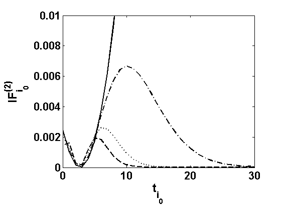
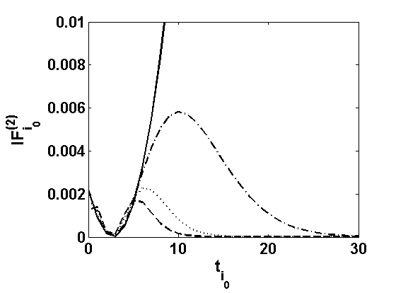
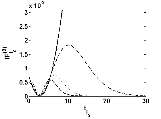
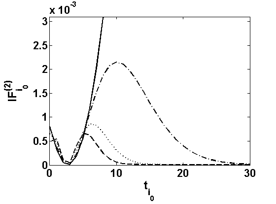
IFi0(2)(ti0;Wτ0,𝐆¯)𝐼superscriptsubscript𝐹subscript𝑖02subscript𝑡subscript𝑖0superscriptsubscript𝑊𝜏0¯𝐆\displaystyle IF_{i_{0}}^{(2)}(t_{i_{0}};W_{\tau}^{0},\underline{\mathbf{G}}) =\displaystyle= 22ϵWτ0(G1,,Gi01,Gi0,ϵ,Gi0+1,,Gn)|ϵ=0.evaluated-atsuperscript2superscript2italic-ϵsuperscriptsubscript𝑊𝜏0subscript𝐺1subscript𝐺subscript𝑖01subscript𝐺subscript𝑖0italic-ϵsubscript𝐺subscript𝑖01subscript𝐺𝑛italic-ϵ0\displaystyle\frac{\partial^{2}}{\partial^{2}\epsilon}W_{\tau}^{0}(G_{1},\cdots,G_{i_{0}-1},G_{i_{0},\epsilon},G_{i_{0}+1},\cdots,G_{n})\big{|}_{\epsilon=0}.

When evaluated at the null model distribution 𝐆¯=𝐅¯𝜽0¯𝐆subscript¯𝐅subscript𝜽0\underline{\mathbf{G}}=\mathbf{\underline{F}}_{{\boldsymbol{\theta}}_{0}}, this second order IF has the simplified form

IFi0(2)(ti0;Wτ0,𝐅¯𝜽0)𝐼superscriptsubscript𝐹subscript𝑖02subscript𝑡subscript𝑖0superscriptsubscript𝑊𝜏0subscript¯𝐅subscript𝜽0\displaystyle IF_{i_{0}}^{(2)}(t_{i_{0}};W_{\tau}^{0},\mathbf{\underline{F}}_{{\boldsymbol{\theta}}_{0}}) =\displaystyle= 2IFi0(ti0;𝑻τ,𝐅¯𝜽0)T𝚺τ1(𝜽0)IFi0(ti0;𝑻τ,𝐅¯𝜽0)2𝐼subscript𝐹subscript𝑖0superscriptsubscript𝑡subscript𝑖0subscript𝑻𝜏subscript¯𝐅subscript𝜽0𝑇superscriptsubscript𝚺𝜏1subscript𝜽0𝐼subscript𝐹subscript𝑖0subscript𝑡subscript𝑖0subscript𝑻𝜏subscript¯𝐅subscript𝜽0\displaystyle 2IF_{i_{0}}(t_{i_{0}};\boldsymbol{T}_{\tau},\mathbf{\underline{F}}_{{\boldsymbol{\theta}}_{0}})^{T}\boldsymbol{\Sigma}_{{\tau}}^{-1}(\boldsymbol{\theta}_{0})IF_{i_{0}}(t_{i_{0}};\boldsymbol{T}_{\tau},\mathbf{\underline{F}}_{{\boldsymbol{\theta}}_{0}}) (30)
=\displaystyle= 2[1n𝑫τ,i0(ti0;𝜽0)]T[𝚿n,τ1(𝜽0)𝚺τ1(𝜽0)𝚿n,τ1(𝜽0)][1n𝑫τ,i0(ti0;𝜽0)].2superscriptdelimited-[]1𝑛subscript𝑫𝜏subscript𝑖0subscript𝑡subscript𝑖0subscript𝜽0𝑇delimited-[]superscriptsubscript𝚿𝑛𝜏1subscript𝜽0superscriptsubscript𝚺𝜏1subscript𝜽0superscriptsubscript𝚿𝑛𝜏1subscript𝜽0delimited-[]1𝑛subscript𝑫𝜏subscript𝑖0subscript𝑡subscript𝑖0subscript𝜽0\displaystyle 2\left[\frac{1}{n}\boldsymbol{D}_{\tau,i_{0}}(t_{i_{0}};{\boldsymbol{\theta}}_{0})\right]^{T}\left[\boldsymbol{\Psi}_{n,\tau}^{-1}({\boldsymbol{\theta}}_{0})\boldsymbol{\Sigma}_{{\tau}}^{-1}(\boldsymbol{\theta}_{0})\boldsymbol{\Psi}_{n,\tau}^{-1}({\boldsymbol{\theta}}_{0})\right]\left[\frac{1}{n}\boldsymbol{D}_{\tau,i_{0}}(t_{i_{0}};{\boldsymbol{\theta}}_{0})\right].

Similarly, we can derive the first and second order IF of Wτ0superscriptsubscript𝑊𝜏0W_{\tau}^{0} for contamination in all directions at the point 𝒕=(t1,,tn)𝒕subscript𝑡1subscript𝑡𝑛\boldsymbol{t}=(t_{1},\ldots,t_{n}) respectively defined as

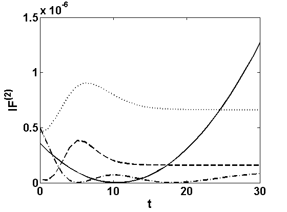
IF(𝒕;Wτ0,𝐆¯)=ϵWτ0(G1,ϵ,,Gn,ϵ)|ϵ=0, and IF(2)(𝒕;Wτ0,𝐆¯)=22ϵWτ0(G1,ϵ,,Gn,ϵ)|ϵ=0.formulae-sequence𝐼𝐹𝒕superscriptsubscript𝑊𝜏0¯𝐆evaluated-atitalic-ϵsuperscriptsubscript𝑊𝜏0subscript𝐺1italic-ϵsubscript𝐺𝑛italic-ϵitalic-ϵ0 and 𝐼superscript𝐹2𝒕superscriptsubscript𝑊𝜏0¯𝐆evaluated-atsuperscript2superscript2italic-ϵsuperscriptsubscript𝑊𝜏0subscript𝐺1italic-ϵsubscript𝐺𝑛italic-ϵitalic-ϵ0\displaystyle IF(\boldsymbol{t};W_{\tau}^{0},\underline{\mathbf{G}})=\frac{\partial}{\partial\epsilon}W_{\tau}^{0}(G_{1,\epsilon},\cdots,G_{n,\epsilon})\big{|}_{\epsilon=0},\mbox{ and }~{}IF^{(2)}(\boldsymbol{t};W_{\tau}^{0},\underline{\mathbf{G}})=\frac{\partial^{2}}{\partial^{2}\epsilon}W_{\tau}^{0}(G_{1,\epsilon},\cdots,G_{n,\epsilon})\big{|}_{\epsilon=0}.

A direct calculation shows that, at the simple null model distribution 𝐆¯=𝐅¯𝜽0¯𝐆subscript¯𝐅subscript𝜽0\underline{\mathbf{G}}=\mathbf{\underline{F}}_{{\boldsymbol{\theta}}_{0}}, these IFs simplifies to

IF(𝒕;Wτ0,𝐅¯𝜽0)𝐼𝐹𝒕superscriptsubscript𝑊𝜏0subscript¯𝐅subscript𝜽0\displaystyle IF(\boldsymbol{t};W_{\tau}^{0},\mathbf{\underline{F}}_{{\boldsymbol{\theta}}_{0}}) =\displaystyle= 0,0\displaystyle 0,
IF(2)(𝒕;Wτ0,𝐅¯𝜽0)𝐼superscript𝐹2𝒕superscriptsubscript𝑊𝜏0subscript¯𝐅subscript𝜽0\displaystyle IF^{(2)}(\boldsymbol{t};W_{\tau}^{0},\mathbf{\underline{F}}_{{\boldsymbol{\theta}}_{0}}) =\displaystyle= 2IF(𝒕;𝑻τ,𝐅¯𝜽0)T𝚺τ1(𝜽0)IF(𝒕;𝑻τ,𝐅¯𝜽0)2𝐼𝐹superscript𝒕subscript𝑻𝜏subscript¯𝐅subscript𝜽0𝑇superscriptsubscript𝚺𝜏1subscript𝜽0𝐼𝐹𝒕subscript𝑻𝜏subscript¯𝐅subscript𝜽0\displaystyle 2IF(\boldsymbol{t};\boldsymbol{T}_{\tau},\mathbf{\underline{F}}_{{\boldsymbol{\theta}}_{0}})^{T}\boldsymbol{\Sigma}_{{\tau}}^{-1}(\boldsymbol{\theta}_{0})IF(\boldsymbol{t};\boldsymbol{T}_{\tau},\mathbf{\underline{F}}_{{\boldsymbol{\theta}}_{0}}) (31)
=\displaystyle= 2[1ni=1n𝑫τ,i(ti;𝜽0)]T[𝚿n,τ1(𝜽0)𝚺τ1(𝜽0)𝚿n,τ1(𝜽0)][1ni=1n𝑫τ,i(ti;𝜽0)].2superscriptdelimited-[]1𝑛superscriptsubscript𝑖1𝑛subscript𝑫𝜏𝑖subscript𝑡𝑖subscript𝜽0𝑇delimited-[]superscriptsubscript𝚿𝑛𝜏1subscript𝜽0superscriptsubscript𝚺𝜏1subscript𝜽0superscriptsubscript𝚿𝑛𝜏1subscript𝜽0delimited-[]1𝑛superscriptsubscript𝑖1𝑛subscript𝑫𝜏𝑖subscript𝑡𝑖subscript𝜽0\displaystyle 2\left[\frac{1}{n}\sum_{i=1}^{n}\boldsymbol{D}_{\tau,i}(t_{i};{\boldsymbol{\theta}}_{0})\right]^{T}\left[\boldsymbol{\Psi}_{n,\tau}^{-1}({\boldsymbol{\theta}}_{0})\boldsymbol{\Sigma}_{{\tau}}^{-1}(\boldsymbol{\theta}_{0})\boldsymbol{\Psi}_{n,\tau}^{-1}({\boldsymbol{\theta}}_{0})\right]\left[\frac{1}{n}\sum_{i=1}^{n}\boldsymbol{D}_{\tau,i}(t_{i};{\boldsymbol{\theta}}_{0})\right].

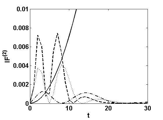
Note that, both the second order IF in (30) and (31) of the Wald-type test functional Wτ0superscriptsubscript𝑊𝜏0W_{\tau}^{0} for testing simple null hypothesis under contamination in one or all directions are bounded, whenever the corresponding MDPDE functional has bounded IF, i.e., for any τ>0𝜏0\tau>0. This implies robustness of our proposed Wald-type tests for simple null hypothesis with τ>0𝜏0\tau>0.

Next we can similarly derive the first and second order IFs of the proposed Wald-type tests functional Wτsubscript𝑊𝜏W_{\tau} in (29) for composite null hypotheses. For brevity, we will skip the details and present only the final results under composite null 𝐆¯=𝐅¯𝜽0¯𝐆subscript¯𝐅subscript𝜽0\underline{\mathbf{G}}=\mathbf{\underline{F}}_{{\boldsymbol{\theta}}_{0}} with 𝜽0Θsubscript𝜽0Θ\boldsymbol{\theta}_{0}\in\Theta. In particular, the first order IF for contamination in either one or all directions are both identically zero, i.e.,

IFi0(ti0;Wτ0,𝐅¯𝜽0)=0,IF(𝒕;Wτ,𝐅¯𝜽0)=0,formulae-sequence𝐼subscript𝐹subscript𝑖0subscript𝑡subscript𝑖0superscriptsubscript𝑊𝜏0subscript¯𝐅subscript𝜽00𝐼𝐹𝒕subscript𝑊𝜏subscript¯𝐅subscript𝜽00IF_{i_{0}}(t_{i_{0}};W_{\tau}^{0},\mathbf{\underline{F}}_{{\boldsymbol{\theta}}_{0}})=0,~{}~{}~{}IF(\boldsymbol{t};W_{\tau},\mathbf{\underline{F}}_{{\boldsymbol{\theta}}_{0}})=0,

and the corresponding second order IF has the form

IFi0(2)(ti0;Wτ,𝐅¯𝜽0)𝐼superscriptsubscript𝐹subscript𝑖02subscript𝑡subscript𝑖0subscript𝑊𝜏subscript¯𝐅subscript𝜽0\displaystyle IF_{i_{0}}^{(2)}(t_{i_{0}};W_{\tau},\mathbf{\underline{F}}_{{\boldsymbol{\theta}}_{0}}) =\displaystyle= 2IFi0(ti0;𝑻τ,𝐅¯𝜽0)T𝑯(𝜽0)[𝑯T(𝜽0)𝚺τ(𝜽0)𝑯(𝜽0)]1𝑯T(𝜽0)IFi0(ti0;𝑻τ,𝐅¯𝜽0)2𝐼subscript𝐹subscript𝑖0superscriptsubscript𝑡subscript𝑖0subscript𝑻𝜏subscript¯𝐅subscript𝜽0𝑇𝑯subscript𝜽0superscriptdelimited-[]superscript𝑯𝑇subscript𝜽0subscript𝚺𝜏subscript𝜽0𝑯subscript𝜽01superscript𝑯𝑇subscript𝜽0𝐼subscript𝐹subscript𝑖0subscript𝑡subscript𝑖0subscript𝑻𝜏subscript¯𝐅subscript𝜽0\displaystyle 2IF_{i_{0}}(t_{i_{0}};\boldsymbol{T}_{\tau},\mathbf{\underline{F}}_{{\boldsymbol{\theta}}_{0}})^{T}\boldsymbol{H}(\boldsymbol{\theta}_{0})\left[\boldsymbol{H}^{T}(\boldsymbol{\theta}_{0})\boldsymbol{\Sigma}_{\tau}(\boldsymbol{\theta}_{0})\boldsymbol{H}(\boldsymbol{\theta}_{0})\right]^{-1}\boldsymbol{H}^{T}(\boldsymbol{\theta}_{0})IF_{i_{0}}(t_{i_{0}};\boldsymbol{T}_{\tau},\mathbf{\underline{F}}_{{\boldsymbol{\theta}}_{0}})
IF(2)(𝒕;Wτ,𝐅¯𝜽0)𝐼superscript𝐹2𝒕subscript𝑊𝜏subscript¯𝐅subscript𝜽0\displaystyle IF^{(2)}(\boldsymbol{t};W_{\tau},\mathbf{\underline{F}}_{{\boldsymbol{\theta}}_{0}}) =\displaystyle= 2IF(𝒕;𝑻τ,𝐅¯𝜽0)T𝑯(𝜽0)[𝑯T(𝜽0)𝚺τ(𝜽0)𝑯(𝜽0)]1𝑯T(𝜽0)IF(𝒕;𝑻τ,𝐅¯𝜽0).2𝐼𝐹superscript𝒕subscript𝑻𝜏subscript¯𝐅subscript𝜽0𝑇𝑯subscript𝜽0superscriptdelimited-[]superscript𝑯𝑇subscript𝜽0subscript𝚺𝜏subscript𝜽0𝑯subscript𝜽01superscript𝑯𝑇subscript𝜽0𝐼𝐹𝒕subscript𝑻𝜏subscript¯𝐅subscript𝜽0\displaystyle 2IF(\boldsymbol{t};\boldsymbol{T}_{\tau},\mathbf{\underline{F}}_{{\boldsymbol{\theta}}_{0}})^{T}\boldsymbol{H}(\boldsymbol{\theta}_{0})\left[\boldsymbol{H}^{T}(\boldsymbol{\theta}_{0})\boldsymbol{\Sigma}_{\tau}(\boldsymbol{\theta}_{0})\boldsymbol{H}(\boldsymbol{\theta}_{0})\right]^{-1}\boldsymbol{H}^{T}(\boldsymbol{\theta}_{0})IF(\boldsymbol{t};\boldsymbol{T}_{\tau},\mathbf{\underline{F}}_{{\boldsymbol{\theta}}_{0}}).

Again these second order IFs are bounded for any τ>0𝜏0\tau>0 and unbounded at τ=0𝜏0\tau=0 implying the robustness of our proposed Wald-type tests for composite hypothesis testing also.

3.2 Level and Power Influence Functions

We will now study the robustness of the level and power of the proposed Wald-type tests through the corresponding influence functions for their asymptotic level and powers (Hampel et al., 1986; Heritier and Ronchetti, 1994; Toma and Broniatowski, 2010; Ghosh and Basu, 2017). Noting the consistency of these proposed Wald-type tests, we consider their asymptotic power under the contiguous alternatives in (14) and (22) respectively for the simple and composite hypotheses. Additionally, considering suitable contamination over these alternatives and the null hypothesis, we define the contaminated distributions, for each i=1,,n𝑖1𝑛i=1,\ldots,n,

Fi,n,ϵ,tiL=(1ϵn)Fi,𝜽0+ϵnti, and Fi,n,ϵ,tiP=(1ϵn)Fi,𝜽n+ϵnti,formulae-sequencesuperscriptsubscript𝐹𝑖𝑛italic-ϵsubscript𝑡𝑖𝐿1italic-ϵ𝑛subscript𝐹𝑖subscript𝜽0limit-fromitalic-ϵ𝑛subscriptsubscript𝑡𝑖 and superscriptsubscript𝐹𝑖𝑛italic-ϵsubscript𝑡𝑖𝑃1italic-ϵ𝑛subscript𝐹𝑖subscript𝜽𝑛limit-fromitalic-ϵ𝑛subscriptsubscript𝑡𝑖F_{i,n,\epsilon,t_{i}}^{L}=\left(1-\frac{\epsilon}{\sqrt{n}}\right)F_{i,{\boldsymbol{\theta}}_{0}}+\frac{\epsilon}{\sqrt{n}}\wedge_{t_{i}},\mbox{ and }F_{i,n,\epsilon,t_{i}}^{P}=\left(1-\frac{\epsilon}{\sqrt{n}}\right)F_{i,{\boldsymbol{\theta}}_{n}}+\frac{\epsilon}{\sqrt{n}}\wedge_{t_{i}},

respectively for the analysis of level and power stability. Denote 𝐭=(t1,,tn)T𝐭superscriptsubscript𝑡1subscript𝑡𝑛𝑇\mathbf{t}=(t_{1},\cdots,t_{n})^{T}, 𝐅¯n,ϵ,𝐭P=(F1,n,ϵ,tiP,,Fn,n,ϵ,tiP)superscriptsubscript¯𝐅𝑛italic-ϵ𝐭𝑃superscriptsubscript𝐹1𝑛italic-ϵsubscript𝑡𝑖𝑃superscriptsubscript𝐹𝑛𝑛italic-ϵsubscript𝑡𝑖𝑃\mathbf{\underline{F}}_{n,\epsilon,\mathbf{t}}^{P}=(F_{1,n,\epsilon,t_{i}}^{P},\cdots,F_{n,n,\epsilon,t_{i}}^{P}) and 𝐅¯n,ϵ,𝐭L=(F1,n,ϵ,tiL,,Fn,n,ϵ,tiL)superscriptsubscript¯𝐅𝑛italic-ϵ𝐭𝐿superscriptsubscript𝐹1𝑛italic-ϵsubscript𝑡𝑖𝐿superscriptsubscript𝐹𝑛𝑛italic-ϵsubscript𝑡𝑖𝐿\mathbf{\underline{F}}_{n,\epsilon,\mathbf{t}}^{L}=(F_{1,n,\epsilon,t_{i}}^{L},\cdots,F_{n,n,\epsilon,t_{i}}^{L}). Then the level influence function (LIF) and the power influence function (PIF) for the proposed Wald-type test statistics Wn0(𝜽0)superscriptsubscript𝑊𝑛0subscript𝜽0W_{n}^{0}(\boldsymbol{\theta}_{0}) for the simple null hypothesis (9) are defined, assuming the nominal level of significance to be α𝛼\alpha, as

LIF(𝐭;Wn0,𝐅¯𝜽0)𝐿𝐼𝐹𝐭superscriptsubscript𝑊𝑛0subscript¯𝐅subscript𝜽0\displaystyle LIF(\mathbf{t};W_{n}^{0},\mathbf{\underline{F}}_{{\boldsymbol{\theta}}_{0}}) =\displaystyle= limnϵP𝐅¯n,ϵ,𝐭L(Wn0(𝜽0)>χp,α2)|ϵ=0,evaluated-atsubscript𝑛italic-ϵsubscript𝑃superscriptsubscript¯𝐅𝑛italic-ϵ𝐭𝐿superscriptsubscript𝑊𝑛0subscript𝜽0superscriptsubscript𝜒𝑝𝛼2italic-ϵ0\displaystyle\lim_{n\rightarrow\infty}~{}\frac{\partial}{\partial\epsilon}P_{\mathbf{\underline{F}}_{n,\epsilon,\mathbf{t}}^{L}}(W_{n}^{0}(\boldsymbol{\theta}_{0})>\chi_{p,\alpha}^{2})\big{|}_{\epsilon=0},
PIF(𝐭;Wn0,𝐅¯𝜽0)𝑃𝐼𝐹𝐭superscriptsubscript𝑊𝑛0subscript¯𝐅subscript𝜽0\displaystyle PIF(\mathbf{t};W_{n}^{0},\mathbf{\underline{F}}_{{\boldsymbol{\theta}}_{0}}) =\displaystyle= limnϵP𝐅¯n,ϵ,𝐭P(Wn0(𝜽0)>χp,α2)|ϵ=0.evaluated-atsubscript𝑛italic-ϵsubscript𝑃superscriptsubscript¯𝐅𝑛italic-ϵ𝐭𝑃superscriptsubscript𝑊𝑛0subscript𝜽0superscriptsubscript𝜒𝑝𝛼2italic-ϵ0\displaystyle\lim_{n\rightarrow\infty}~{}\frac{\partial}{\partial\epsilon}P_{\mathbf{\underline{F}}_{n,\epsilon,\mathbf{t}}^{P}}(W_{n}^{0}(\boldsymbol{\theta}_{0})>\chi_{p,\alpha}^{2})\big{|}_{\epsilon=0}.

Similarly the LIF and PIF of the proposed Wald-type test statistics Wn(𝜽^τ)subscript𝑊𝑛subscript^𝜽𝜏W_{n}(\widehat{\boldsymbol{\theta}}_{\tau}) for the composite null hypothesis (19) can be defined through above expressions by replacing Wn0(𝜽0)superscriptsubscript𝑊𝑛0subscript𝜽0W_{n}^{0}(\boldsymbol{\theta}_{0}) and χp,α2superscriptsubscript𝜒𝑝𝛼2\chi_{p,\alpha}^{2} by Wn(𝜽^τ)subscript𝑊𝑛subscript^𝜽𝜏W_{n}(\widehat{\boldsymbol{\theta}}_{\tau}) and χr,α2superscriptsubscript𝜒𝑟𝛼2\chi_{r,\alpha}^{2} respectively, where 𝜽0subscript𝜽0\boldsymbol{\theta}_{0} is now the true null parameter in Θ0subscriptΘ0\Theta_{0}.

Let us first consider the case of simple null hypothesis and derive the asymptotic power under the contiguous contaminated distribution 𝐅¯n,ϵ,𝐭Psuperscriptsubscript¯𝐅𝑛italic-ϵ𝐭𝑃\mathbf{\underline{F}}_{n,\epsilon,\mathbf{t}}^{P} in the following theorem.

Theorem 9

Consider the problem of testing the simple null hypothesis (9) by the proposed Wald-type test statistics Wn0(𝛉0)superscriptsubscript𝑊𝑛0subscript𝛉0W_{n}^{0}(\boldsymbol{\theta}_{0}) at α𝛼\alpha-level of significance and consider the contiguous alternative hypotheses given by (14). Then the following results hold.

  1. 1.

    The asymptotic distribution of Wn0(𝜽0)superscriptsubscript𝑊𝑛0subscript𝜽0W_{n}^{0}({\boldsymbol{\theta}}_{0}) under 𝐅¯n,ϵ,𝐭Psuperscriptsubscript¯𝐅𝑛italic-ϵ𝐭𝑃\mathbf{\underline{F}}_{n,\epsilon,\mathbf{t}}^{P} is χp2(δϵ)superscriptsubscript𝜒𝑝2subscript𝛿italic-ϵ\chi_{p}^{2}(\delta_{\epsilon}) with

    δϵ=𝒅~ϵ,𝒕,τT(𝜽0)𝚺τ1(𝜽0)𝒅~ϵ,𝒕,τ(𝜽0),subscript𝛿italic-ϵsuperscriptsubscript~𝒅italic-ϵ𝒕𝜏𝑇subscript𝜽0superscriptsubscript𝚺𝜏1subscript𝜽0subscript~𝒅italic-ϵ𝒕𝜏subscript𝜽0\delta_{\epsilon}=\widetilde{\boldsymbol{d}}_{\epsilon,\boldsymbol{t},{\tau}}^{T}(\boldsymbol{\theta}_{0})\boldsymbol{\Sigma}_{{\tau}}^{-1}(\boldsymbol{\theta}_{0})\widetilde{\boldsymbol{d}}_{\epsilon,\boldsymbol{t},{\tau}}(\boldsymbol{\theta}_{0}),

    where 𝒅~ϵ,𝒕,τ(𝜽0)=𝒅+ϵIF(𝒕;𝑻τ,𝐅¯𝜽0)subscript~𝒅italic-ϵ𝒕𝜏subscript𝜽0𝒅italic-ϵ𝐼𝐹𝒕subscript𝑻𝜏subscript¯𝐅subscript𝜽0\widetilde{\boldsymbol{d}}_{\epsilon,\boldsymbol{t},{\tau}}(\boldsymbol{\theta}_{0})=\boldsymbol{d}+\epsilon IF(\boldsymbol{t};\boldsymbol{T}_{\tau},\mathbf{\underline{F}}_{{\boldsymbol{\theta}}_{0}}) with IF(𝒕;𝑻τ,𝐅¯𝜽0)𝐼𝐹𝒕subscript𝑻𝜏subscript¯𝐅subscript𝜽0IF(\boldsymbol{t};\boldsymbol{T}_{\tau},\mathbf{\underline{F}}_{{\boldsymbol{\theta}}_{0}}) being given by (27).

  2. 2.

    The corresponding asymptotic power under contiguous contaminated distribution 𝐅¯n,ϵ,𝐭Psuperscriptsubscript¯𝐅𝑛italic-ϵ𝐭𝑃\mathbf{\underline{F}}_{n,\epsilon,\mathbf{t}}^{P} is given by

    πWn0(𝜽n,ϵ,𝒕)subscript𝜋superscriptsubscript𝑊𝑛0subscript𝜽𝑛italic-ϵ𝒕\displaystyle{\pi}_{W_{n}^{0}}(\boldsymbol{\theta}_{n},\epsilon,\boldsymbol{t}) =limnP𝐅¯n,ϵ,𝐭P(Wn0(𝜽0)>χp,α2)=1Gχp2(δϵ)(χp,α2)absentsubscript𝑛subscript𝑃superscriptsubscript¯𝐅𝑛italic-ϵ𝐭𝑃superscriptsubscript𝑊𝑛0subscript𝜽0superscriptsubscript𝜒𝑝𝛼21subscript𝐺superscriptsubscript𝜒𝑝2subscript𝛿italic-ϵsuperscriptsubscript𝜒𝑝𝛼2\displaystyle=\lim_{n\rightarrow\infty}P_{\mathbf{\underline{F}}_{n,\epsilon,\mathbf{t}}^{P}}(W_{n}^{0}(\boldsymbol{\theta}_{0})>\chi_{p,\alpha}^{2})=1-G_{\chi_{p}^{2}(\delta_{\epsilon})}(\chi_{p,\alpha}^{2})
    =v=0Cv(𝒅~ϵ,𝒕,τ(𝜽0),𝚺τ1(𝜽0))P(χp+2v2>χp,α2),absentsuperscriptsubscript𝑣0subscript𝐶𝑣subscript~𝒅italic-ϵ𝒕𝜏subscript𝜽0superscriptsubscript𝚺𝜏1subscript𝜽0𝑃superscriptsubscript𝜒𝑝2𝑣2superscriptsubscript𝜒𝑝𝛼2\displaystyle=\sum\limits_{v=0}^{\infty}C_{v}\left(\widetilde{\boldsymbol{d}}_{\epsilon,\boldsymbol{t},{\tau}}(\boldsymbol{\theta}_{0}),\boldsymbol{\Sigma}_{{\tau}}^{-1}(\boldsymbol{\theta}_{0})\right)P\left(\chi_{p+2v}^{2}>\chi_{p,\alpha}^{2}\right), (32)

    where Cv(𝒔,𝑨)=(𝐬T𝑨𝐬)vv!2ve12𝐬T𝑨𝐬.subscript𝐶𝑣𝒔𝑨superscriptsuperscript𝐬𝑇𝑨𝐬𝑣𝑣superscript2𝑣superscript𝑒12superscript𝐬𝑇𝑨𝐬C_{v}\left(\boldsymbol{s},\boldsymbol{A}\right)=\frac{\left(\mathbf{s}^{T}\boldsymbol{A}\mathbf{s}\right)^{v}}{v!2^{v}}e^{-\frac{1}{2}\mathbf{s}^{T}\boldsymbol{A}\mathbf{s}}.

Proof. Denote 𝛉n=𝐓τ(𝐅¯n,ϵ,𝐭P)superscriptsubscript𝛉nsubscript𝐓τsuperscriptsubscript¯𝐅nϵ𝐭P\boldsymbol{\theta}_{n}^{\ast}=\boldsymbol{T}_{\tau}(\mathbf{\underline{F}}_{n,\epsilon,\mathbf{t}}^{P}). Then, we can express our Wald-type test statistics in (10) as

Wn0(𝜽0)=n(𝜽^τ𝜽0)T𝚺τ1(𝜽0)(𝜽^τ𝜽0)superscriptsubscript𝑊𝑛0subscript𝜽0𝑛superscriptsubscript^𝜽𝜏subscript𝜽0𝑇superscriptsubscript𝚺𝜏1subscript𝜽0subscript^𝜽𝜏subscript𝜽0\displaystyle W_{n}^{0}(\boldsymbol{\theta}_{0})=n(\widehat{\boldsymbol{\theta}}_{\tau}-\boldsymbol{\theta}_{0})^{T}\boldsymbol{\Sigma}_{\tau}^{-1}(\boldsymbol{\theta}_{0})(\widehat{\boldsymbol{\theta}}_{\tau}-\boldsymbol{\theta}_{0}) (33)
=\displaystyle= n(𝜽^τ𝜽n)T𝚺τ1(𝜽0)(𝜽^τ𝜽n)+2n(𝜽^τ𝜽n)T𝚺τ1(𝜽0)(𝜽n𝜽0)+n(𝜽n𝜽0)T𝚺τ1(𝜽0)(𝜽n𝜽0).𝑛superscriptsubscript^𝜽𝜏superscriptsubscript𝜽𝑛𝑇superscriptsubscript𝚺𝜏1subscript𝜽0subscript^𝜽𝜏superscriptsubscript𝜽𝑛2𝑛superscriptsubscript^𝜽𝜏superscriptsubscript𝜽𝑛𝑇superscriptsubscript𝚺𝜏1subscript𝜽0superscriptsubscript𝜽𝑛subscript𝜽0𝑛superscriptsuperscriptsubscript𝜽𝑛subscript𝜽0𝑇superscriptsubscript𝚺𝜏1subscript𝜽0superscriptsubscript𝜽𝑛subscript𝜽0\displaystyle n(\widehat{\boldsymbol{\theta}}_{\tau}-\boldsymbol{\theta}_{n}^{\ast})^{T}\boldsymbol{\Sigma}_{\tau}^{-1}(\boldsymbol{\theta}_{0})(\widehat{\boldsymbol{\theta}}_{\tau}-\boldsymbol{\theta}_{n}^{\ast})+2n(\widehat{\boldsymbol{\theta}}_{\tau}-\boldsymbol{\theta}_{n}^{\ast})^{T}\boldsymbol{\Sigma}_{\tau}^{-1}(\boldsymbol{\theta}_{0})(\boldsymbol{\theta}_{n}^{\ast}-\boldsymbol{\theta}_{0})+n(\boldsymbol{\theta}_{n}^{\ast}-\boldsymbol{\theta}_{0})^{T}\boldsymbol{\Sigma}_{\tau}^{-1}(\boldsymbol{\theta}_{0})(\boldsymbol{\theta}_{n}^{\ast}-\boldsymbol{\theta}_{0}).~{}~{}~{}~{}~{}~{}

A suitable Taylor series expansion of 𝛉nsuperscriptsubscript𝛉𝑛\boldsymbol{\theta}_{n}^{\ast}, as a function of ϵitalic-ϵ\epsilon at ϵn=0subscriptitalic-ϵ𝑛0\epsilon_{n}=0 yields (Ghosh et al., 2016)

𝜽nsuperscriptsubscript𝜽𝑛\displaystyle\boldsymbol{\theta}_{n}^{\ast} =𝜽n+ϵnIF(𝒕;𝑻τ,𝐅¯𝜽0)+op(1n𝟏p)absentsubscript𝜽𝑛italic-ϵ𝑛𝐼𝐹𝒕subscript𝑻𝜏subscript¯𝐅subscript𝜽0subscript𝑜𝑝1𝑛subscript1𝑝\displaystyle=\boldsymbol{\theta}_{n}+\tfrac{\epsilon}{\sqrt{n}}IF(\boldsymbol{t};\boldsymbol{T}_{\tau},\mathbf{\underline{F}}_{{\boldsymbol{\theta}}_{0}})+o_{p}(\frac{1}{\sqrt{n}}\boldsymbol{1}_{p})

and hence

n(𝜽n𝜽n)𝑛superscriptsubscript𝜽𝑛subscript𝜽𝑛\displaystyle\sqrt{n}(\boldsymbol{\theta}_{n}^{\ast}-\boldsymbol{\theta}_{n}) =ϵIF(𝒕;𝑻τ,𝐅¯𝜽0)+op(𝟏p),absentitalic-ϵ𝐼𝐹𝒕subscript𝑻𝜏subscript¯𝐅subscript𝜽0subscript𝑜𝑝subscript1𝑝\displaystyle=\epsilon IF(\boldsymbol{t};\boldsymbol{T}_{\tau},\mathbf{\underline{F}}_{{\boldsymbol{\theta}}_{0}})+o_{p}(\boldsymbol{1}_{p}),
n(𝜽n𝜽0n1/2𝒅)𝑛superscriptsubscript𝜽𝑛subscript𝜽0superscript𝑛12𝒅\displaystyle\sqrt{n}(\boldsymbol{\theta}_{n}^{\ast}-\boldsymbol{\theta}_{0}-n^{-1/2}\boldsymbol{d}) =ϵIF(𝒕;𝑻τ,𝐅¯𝜽0)+op(𝟏p).absentitalic-ϵ𝐼𝐹𝒕subscript𝑻𝜏subscript¯𝐅subscript𝜽0subscript𝑜𝑝subscript1𝑝\displaystyle=\epsilon IF(\boldsymbol{t};\boldsymbol{T}_{\tau},\mathbf{\underline{F}}_{{\boldsymbol{\theta}}_{0}})+o_{p}(\boldsymbol{1}_{p}).

Writing 𝛉nsuperscriptsubscript𝛉𝑛\boldsymbol{\theta}_{n}^{\ast} in terms of 𝛉0subscript𝛉0\boldsymbol{\theta}_{0}, we get

n(𝜽n𝜽0)𝑛superscriptsubscript𝜽𝑛subscript𝜽0\displaystyle\sqrt{n}(\boldsymbol{\theta}_{n}^{\ast}-\boldsymbol{\theta}_{0}) =𝒅+ϵIF(𝒕;𝑻τ,𝐅¯𝜽0)+op(𝟏p)absent𝒅italic-ϵ𝐼𝐹𝒕subscript𝑻𝜏subscript¯𝐅subscript𝜽0subscript𝑜𝑝subscript1𝑝\displaystyle=\boldsymbol{d}+\epsilon IF(\boldsymbol{t};\boldsymbol{T}_{\tau},\mathbf{\underline{F}}_{{\boldsymbol{\theta}}_{0}})+o_{p}(\boldsymbol{1}_{p})
=𝒅~ϵ,𝒕,τ(𝜽0)+op(𝟏p).absentsubscript~𝒅italic-ϵ𝒕𝜏subscript𝜽0subscript𝑜𝑝subscript1𝑝\displaystyle=\widetilde{\boldsymbol{d}}_{\epsilon,\boldsymbol{t},\tau}(\boldsymbol{\theta}_{0})+o_{p}(\boldsymbol{1}_{p}). (34)

Using these, we can rewrite (33) as

Wn0(𝜽0)=n(n(𝜽^τ𝜽n)+𝒅~ϵ,𝒙,τ(𝜽0))T𝚺τ1(𝜽0)(n(𝜽^τ𝜽n)+𝒅~ϵ,𝒙,τ(𝜽0))+op(1).superscriptsubscript𝑊𝑛0subscript𝜽0𝑛superscript𝑛subscript^𝜽𝜏superscriptsubscript𝜽𝑛subscript~𝒅italic-ϵ𝒙𝜏subscript𝜽0𝑇superscriptsubscript𝚺𝜏1subscript𝜽0𝑛subscript^𝜽𝜏superscriptsubscript𝜽𝑛subscript~𝒅italic-ϵ𝒙𝜏subscript𝜽0subscript𝑜𝑝1\displaystyle W_{n}^{0}(\boldsymbol{\theta}_{0})=n\left(\sqrt{n}(\widehat{\boldsymbol{\theta}}_{\tau}-\boldsymbol{\theta}_{n}^{\ast})+\widetilde{\boldsymbol{d}}_{\epsilon,\boldsymbol{x},\tau}(\boldsymbol{\theta}_{0})\right)^{T}\boldsymbol{\Sigma}_{\tau}^{-1}(\boldsymbol{\theta}_{0})\left(\sqrt{n}(\widehat{\boldsymbol{\theta}}_{\tau}-\boldsymbol{\theta}_{n}^{\ast})+\widetilde{\boldsymbol{d}}_{\epsilon,\boldsymbol{x},\tau}(\boldsymbol{\theta}_{0})\right)+o_{p}(1). (35)

But, under 𝐅¯n,ϵ,𝐭Psuperscriptsubscript¯𝐅𝑛italic-ϵ𝐭𝑃\mathbf{\underline{F}}_{n,\epsilon,\mathbf{t}}^{P}, the asymptotic distribution of MDPDE and continuity of 𝚺τ(𝛉)subscript𝚺𝜏𝛉\boldsymbol{\Sigma}_{\tau}(\boldsymbol{\theta}) implies that

n(𝜽^τ𝜽n)n𝒩(𝟎p,𝚺τ(𝜽0)).𝑛subscript^𝜽𝜏superscriptsubscript𝜽𝑛𝑛𝒩subscript0𝑝subscript𝚺𝜏subscript𝜽0\sqrt{n}(\widehat{\boldsymbol{\theta}}_{\tau}-\boldsymbol{\theta}_{n}^{\ast})\underset{n\rightarrow\infty}{\overset{\mathcal{L}}{\longrightarrow}}\mathcal{N}(\boldsymbol{0}_{p},\boldsymbol{\Sigma}_{\tau}(\boldsymbol{\theta}_{0})). (36)

Hence combining (35) and (36), we finally get

Wn0(𝜽^τ)nχp2(δϵ)superscriptsubscript𝑊𝑛0subscript^𝜽𝜏𝑛superscriptsubscript𝜒𝑝2subscript𝛿italic-ϵW_{n}^{0}(\widehat{\boldsymbol{\theta}}_{\tau})\underset{n\rightarrow\infty}{\overset{\mathcal{L}}{\longrightarrow}}\chi_{p}^{2}\left(\delta_{\epsilon}\right)

with δϵsubscript𝛿italic-ϵ\delta_{\epsilon} as defined in the statement of the theorem. This completes the proof of Part 1 of the theorem.

Next, Part 2 of the theorem follows directly from the infinite series expansion of non-central distribution functions in terms of that of the central chi-square variables as follows:

πWn0(𝜽n,ϵ,𝒕)subscript𝜋superscriptsubscript𝑊𝑛0subscript𝜽𝑛italic-ϵ𝒕\displaystyle{\pi}_{W_{n}^{0}}(\boldsymbol{\theta}_{n},\epsilon,\boldsymbol{t}) =limnP𝐅¯n,ϵ,𝐭P(Wn0(𝜽0)>χp,α2)absentsubscript𝑛subscript𝑃superscriptsubscript¯𝐅𝑛italic-ϵ𝐭𝑃superscriptsubscript𝑊𝑛0subscript𝜽0superscriptsubscript𝜒𝑝𝛼2\displaystyle=\lim_{n\rightarrow\infty}P_{\mathbf{\underline{F}}_{n,\epsilon,\mathbf{t}}^{P}}(W_{n}^{0}(\boldsymbol{\theta}_{0})>\chi_{p,\alpha}^{2})
=P(χp2(δϵ)>χp,α2)=1Gχp2(δϵ)(χp,α2)absent𝑃superscriptsubscript𝜒𝑝2subscript𝛿italic-ϵsuperscriptsubscript𝜒𝑝𝛼21subscript𝐺superscriptsubscript𝜒𝑝2subscript𝛿italic-ϵsuperscriptsubscript𝜒𝑝𝛼2\displaystyle=P(\chi_{p}^{2}\left(\delta_{\epsilon}\right)>\chi_{p,\alpha}^{2})=1-G_{\chi_{p}^{2}\left(\delta_{\epsilon}\right)}\left(\chi_{p,\alpha}^{2}\right)
=v=0Cv(𝒅~ϵ,𝒕,τ(𝜽0),𝚺τ1(𝜽0))P(χp+2v2>χp,α2).absentsuperscriptsubscript𝑣0subscript𝐶𝑣subscript~𝒅italic-ϵ𝒕𝜏subscript𝜽0superscriptsubscript𝚺𝜏1subscript𝜽0𝑃superscriptsubscript𝜒𝑝2𝑣2superscriptsubscript𝜒𝑝𝛼2\displaystyle=\sum\limits_{v=0}^{\infty}C_{v}\left(\widetilde{\boldsymbol{d}}_{\epsilon,\boldsymbol{t},{\tau}}(\boldsymbol{\theta}_{0}),\boldsymbol{\Sigma}_{{\tau}}^{-1}(\boldsymbol{\theta}_{0})\right)P\left(\chi_{p+2v}^{2}>\chi_{p,\alpha}^{2}\right).


Note that, substituting ϵ=0italic-ϵ0\epsilon=0 in Expression (32) of the above theorem, we have an infinite series expression for the asymptotic power of the proposed Wald-type tests under the contiguous alternative hypotheses (14) as given by

πWn0(𝜽n)=πWn0(𝜽n,0,𝒕)=v=0Cv(𝒅,𝚺τ1(𝜽0))P(χp+2v2>χp,α2),subscript𝜋superscriptsubscript𝑊𝑛0subscript𝜽𝑛subscript𝜋superscriptsubscript𝑊𝑛0subscript𝜽𝑛0𝒕superscriptsubscript𝑣0subscript𝐶𝑣𝒅superscriptsubscript𝚺𝜏1subscript𝜽0𝑃superscriptsubscript𝜒𝑝2𝑣2superscriptsubscript𝜒𝑝𝛼2{\pi}_{W_{n}^{0}}(\boldsymbol{\theta}_{n})={\pi}_{W_{n}^{0}}(\boldsymbol{\theta}_{n},0,\boldsymbol{t})=\sum\limits_{v=0}^{\infty}C_{v}\left(\boldsymbol{d},\boldsymbol{\Sigma}_{{\tau}}^{-1}(\boldsymbol{\theta}_{0})\right)P\left(\chi_{p+2v}^{2}>\chi_{p,\alpha}^{2}\right),

which has been previously obtained in terms of suitable distribution function in (16).

Further, substituting 𝒅=𝟎p𝒅subscript0𝑝\boldsymbol{d}=\boldsymbol{0}_{p} in Expression (32), we get the asymptotic level of the proposed Wald-type tests under the contaminated distribution 𝐅¯n,ϵ,𝐭Lsuperscriptsubscript¯𝐅𝑛italic-ϵ𝐭𝐿\mathbf{\underline{F}}_{n,\epsilon,\mathbf{t}}^{L} as given by

αWn0(ϵ,𝒕)subscript𝛼superscriptsubscript𝑊𝑛0italic-ϵ𝒕\displaystyle\alpha_{W_{n}^{0}}(\epsilon,\boldsymbol{t}) =πWn0(𝜽0,ϵ,𝒕)|𝒅=𝟎p=v=0Cv(ϵIF(𝒕;𝑻τ,𝐅¯𝜽0),𝚺τ1(𝜽0))P(χp+2v2>χp,α2).absentevaluated-atsubscript𝜋superscriptsubscript𝑊𝑛0subscript𝜽0italic-ϵ𝒕𝒅subscript0𝑝superscriptsubscript𝑣0subscript𝐶𝑣italic-ϵ𝐼𝐹𝒕subscript𝑻𝜏subscript¯𝐅subscript𝜽0superscriptsubscript𝚺𝜏1subscript𝜽0𝑃superscriptsubscript𝜒𝑝2𝑣2superscriptsubscript𝜒𝑝𝛼2\displaystyle={\pi}_{W_{n}^{0}}(\boldsymbol{\theta}_{0},\epsilon,\boldsymbol{t})\big{|}_{\boldsymbol{d}=\boldsymbol{0}_{p}}=\sum\limits_{v=0}^{\infty}C_{v}\left(\epsilon IF(\boldsymbol{t};\boldsymbol{T}_{\tau},\mathbf{\underline{F}}_{{\boldsymbol{\theta}}_{0}}),\boldsymbol{\Sigma}_{{\tau}}^{-1}(\boldsymbol{\theta}_{0})\right)P\left(\chi_{p+2v}^{2}>\chi_{p,\alpha}^{2}\right).

Finally, using the expression of the asymptotic power πWn0(𝜽0,ϵ,𝒕)subscript𝜋superscriptsubscript𝑊𝑛0subscript𝜽0italic-ϵ𝒕{\pi}_{W_{n}^{0}}(\boldsymbol{\theta}_{0},\epsilon,\boldsymbol{t}) from (32) and differentiating it suitably, we get the required PIF and then get the LIF by substituting 𝒅=𝟎p𝒅subscript0𝑝\boldsymbol{d}=\boldsymbol{0}_{p} as presented in the following theorem.

Theorem 10

Under the assumptions of Theorem 9, the power and level influence functions of the proposed Wald-type tests for the simple null hypothesis (9) are given by

PIF(𝐭;Wn0,𝐅¯𝜽0)=Kp(𝐝T𝚺τ1(𝜽0)𝐝)𝒅T𝚺τ1(𝜽0)IF(𝒕;𝑻τ,𝐅¯𝜽0),𝑃𝐼𝐹𝐭superscriptsubscript𝑊𝑛0subscript¯𝐅subscript𝜽0superscriptsubscript𝐾𝑝superscript𝐝𝑇superscriptsubscript𝚺𝜏1subscript𝜽0𝐝superscript𝒅𝑇superscriptsubscript𝚺𝜏1subscript𝜽0𝐼𝐹𝒕subscript𝑻𝜏subscript¯𝐅subscript𝜽0PIF(\mathbf{t};W_{n}^{0},\mathbf{\underline{F}}_{{\boldsymbol{\theta}}_{0}})=K_{p}^{\ast}\left(\mathbf{d}^{T}\boldsymbol{\Sigma}_{{\tau}}^{-1}(\boldsymbol{\theta}_{0})\mathbf{d}\right)\boldsymbol{d}^{T}\boldsymbol{\Sigma}_{{\tau}}^{-1}(\boldsymbol{\theta}_{0})IF(\boldsymbol{t};\boldsymbol{T}_{\tau},\mathbf{\underline{F}}_{{\boldsymbol{\theta}}_{0}}),

with Kp(s)=es2v=0sv1v!2v(2vs)P(χp+2v2>χp,τ2)superscriptsubscript𝐾𝑝𝑠superscript𝑒𝑠2superscriptsubscript𝑣0superscript𝑠𝑣1𝑣superscript2𝑣2𝑣𝑠𝑃superscriptsubscript𝜒𝑝2𝑣2superscriptsubscript𝜒𝑝𝜏2K_{p}^{\ast}(s)=e^{-\frac{s}{2}}\sum\limits_{v=0}^{\infty}\frac{s^{v-1}}{v!2^{v}}(2v-s)P\left(\chi_{p+2v}^{2}>\chi_{p,\tau}^{2}\right) and

LIF(𝐭;Wn0,𝐅¯𝜽0)=0.𝐿𝐼𝐹𝐭superscriptsubscript𝑊𝑛0subscript¯𝐅subscript𝜽00LIF(\mathbf{t};W_{n}^{0},\mathbf{\underline{F}}_{{\boldsymbol{\theta}}_{0}})=0.

Proof. Considering the expression of πWn0(𝜽0,ϵ,𝒕)subscript𝜋superscriptsubscript𝑊𝑛0subscript𝜽0italic-ϵ𝒕{\pi}_{W_{n}^{0}}(\boldsymbol{\theta}_{0},\epsilon,\boldsymbol{t}) from (32) in Theorem 9 and using the definition of the PIF along with the chain rule of derivatives, we get

PIF(𝐭;Wn0,𝐅¯𝜽0)𝑃𝐼𝐹𝐭superscriptsubscript𝑊𝑛0subscript¯𝐅subscript𝜽0\displaystyle PIF(\mathbf{t};W_{n}^{0},\mathbf{\underline{F}}_{{\boldsymbol{\theta}}_{0}}) =\displaystyle= ϵπWn0(𝜽0,ϵ,𝒕)|ϵ=0evaluated-atitalic-ϵsubscript𝜋superscriptsubscript𝑊𝑛0subscript𝜽0italic-ϵ𝒕italic-ϵ0\displaystyle\frac{\partial}{\partial\epsilon}\left.{\pi}_{W_{n}^{0}}(\boldsymbol{\theta}_{0},\epsilon,\boldsymbol{t})\right|_{\epsilon=0} (37)
=\displaystyle= v=0ϵCv(𝒅~ϵ,𝒕,τ(𝜽0),𝚺τ1(𝜽0))|ϵ=0P(χp+2v2>χp,α2)evaluated-atsuperscriptsubscript𝑣0italic-ϵsubscript𝐶𝑣subscript~𝒅italic-ϵ𝒕𝜏subscript𝜽0superscriptsubscript𝚺𝜏1subscript𝜽0italic-ϵ0𝑃superscriptsubscript𝜒𝑝2𝑣2superscriptsubscript𝜒𝑝𝛼2\displaystyle\sum\limits_{v=0}^{\infty}\frac{\partial}{\partial\epsilon}\left.C_{v}\left(\widetilde{\boldsymbol{d}}_{\epsilon,\boldsymbol{t},{\tau}}(\boldsymbol{\theta}_{0}),\boldsymbol{\Sigma}_{{\tau}}^{-1}(\boldsymbol{\theta}_{0})\right)\right|_{\epsilon=0}P\left(\chi_{p+2v}^{2}>\chi_{p,\alpha}^{2}\right)
=\displaystyle= v=0{𝐬Cv(𝐬,𝚺τ1(𝜽0))|𝐬=𝒅~0,𝒕,τ(𝜽0)}T{ϵ𝒅~ϵ,𝒕,τ(𝜽0)|ϵ=0}P(χp+2v2>χp,α2).superscriptsubscript𝑣0superscriptevaluated-at𝐬subscript𝐶𝑣𝐬superscriptsubscript𝚺𝜏1subscript𝜽0𝐬subscript~𝒅0𝒕𝜏subscript𝜽0𝑇evaluated-atitalic-ϵsubscript~𝒅italic-ϵ𝒕𝜏subscript𝜽0italic-ϵ0𝑃superscriptsubscript𝜒𝑝2𝑣2superscriptsubscript𝜒𝑝𝛼2\displaystyle\sum\limits_{v=0}^{\infty}\left\{\frac{\partial}{\partial\mathbf{s}}\left.C_{v}\left(\mathbf{s},\boldsymbol{\Sigma}_{\tau}^{-1}(\boldsymbol{\theta}_{0})\right)\right|_{\mathbf{s}=\widetilde{\boldsymbol{d}}_{0,\boldsymbol{t},\tau}(\boldsymbol{\theta}_{0})}\right\}^{T}\left\{\frac{\partial}{\partial\epsilon}\left.\widetilde{\boldsymbol{d}}_{\epsilon,\boldsymbol{t},\tau}(\boldsymbol{\theta}_{0})\right|_{\epsilon=0}\right\}P\left(\chi_{p+2v}^{2}>\chi_{p,\alpha}^{2}\right).~{}~{}~{}~{}~{}

Now, one can check that 𝒅~0,𝒙,τ(𝜽0)=𝒅subscript~𝒅0𝒙𝜏subscript𝜽0𝒅\widetilde{\boldsymbol{d}}_{0,\boldsymbol{x},\tau}(\boldsymbol{\theta}_{0})=\boldsymbol{d}, ϵ𝒅~ϵ,𝒕,τ(𝜽0)=IF(𝒕;𝑻τ,𝐅¯𝜽0)italic-ϵsubscript~𝒅italic-ϵ𝒕𝜏subscript𝜽0𝐼𝐹𝒕subscript𝑻𝜏subscript¯𝐅subscript𝜽0\frac{\partial}{\partial\epsilon}\widetilde{\boldsymbol{d}}_{\epsilon,\boldsymbol{t},\tau}(\boldsymbol{\theta}_{0})=IF(\boldsymbol{t};\boldsymbol{T}_{\tau},\mathbf{\underline{F}}_{{\boldsymbol{\theta}}_{0}}) and

𝐭Cv(𝐭,𝐀)=(𝐭T𝐀𝐭)v1v!2v(2v𝐭T𝐀𝐭)𝐀𝐭e12𝐭T𝐀𝐭.𝐭subscript𝐶𝑣𝐭𝐀superscriptsuperscript𝐭𝑇𝐀𝐭𝑣1𝑣superscript2𝑣2𝑣superscript𝐭𝑇𝐀𝐭𝐀𝐭superscript𝑒12superscript𝐭𝑇𝐀𝐭\frac{\partial}{\partial\mathbf{t}}C_{v}\left(\mathbf{t},\mathbf{A}\right)=\frac{\left(\mathbf{t}^{T}\mathbf{A}\mathbf{t}\right)^{v-1}}{v!2^{v}}\left(2v-\mathbf{t}^{T}\mathbf{A}\mathbf{t}\right)\mathbf{A}\mathbf{t}e^{-\frac{1}{2}\mathbf{t}^{T}\mathbf{A}\mathbf{t}}.

Substituting these expressions in (37) and simplifying, we obtain the required expression of the PIF as given in the theorem.

Finally, the LIF follows from the PIF by substituting 𝒅=𝟎p𝒅subscript0𝑝\boldsymbol{d}=\boldsymbol{0}_{p}.    


Note that the above PIF is clearly bounded if and only if the IF of the MDPDE functional 𝑻τsubscript𝑻𝜏\boldsymbol{T}_{\tau} is bounded, i.e., whenever τ>0𝜏0\tau>0. This again implies the robustness of the asymptotic power of the proposed Wald-type tests with τ>0𝜏0\tau>0 under contiguous contamination, over the classical MLE based Wald test (at τ=0𝜏0\tau=0) that has an unbounded PIF. Further, the asymptotic level of the Wald-type tests will not also be affected by a contiguous contamination as suggested by its zero LIF.

Next we can similarly derive the PIF and LIF for the proposed Wald-type test statistics Wn(𝜽^τ)subscript𝑊𝑛subscript^𝜽𝜏W_{n}(\widehat{\boldsymbol{\theta}}_{\tau}) for composite null hypotheses also. For brevity, we only present the main results corresponding to Theorem 9 and 10 for the composite hypotheses case in the following theorems; proofs are similar and hence omitted. The main implications are again the same proving the claimed robustness of our proposal with τ>0𝜏0\tau>0 in terms of its asymptotic level and power under contiguous contamination through zero LIF and bounded PIF.

Theorem 11

Consider the problem of testing the composite null hypothesis (19) by the proposed Wald-type test statistics Wn(𝛉^τ)subscript𝑊𝑛subscript^𝛉𝜏W_{n}(\widehat{\boldsymbol{\theta}}_{\tau}) at α𝛼\alpha-level of significance and consider the contiguous alternative hypotheses given by (22). Then the following results hold.

  1. 1.

    The asymptotic distribution of Wn(𝜽^τ)subscript𝑊𝑛subscript^𝜽𝜏W_{n}(\widehat{\boldsymbol{\theta}}_{\tau}) under 𝐅¯n,ϵ,𝐭Psuperscriptsubscript¯𝐅𝑛italic-ϵ𝐭𝑃\mathbf{\underline{F}}_{n,\epsilon,\mathbf{t}}^{P} is χr2(δϵ)superscriptsubscript𝜒𝑟2superscriptsubscript𝛿italic-ϵ\chi_{r}^{2}(\delta_{\epsilon}^{\ast}) with

    δϵ=𝒅~ϵ,𝒕,τT(𝜽0)𝑯(𝜽0)[𝑯T(𝜽0)𝚺τ(𝜽0)𝑯(𝜽0)]1𝑯T(𝜽0)𝒅~ϵ,𝒕,τ(𝜽0),superscriptsubscript𝛿italic-ϵsuperscriptsubscript~𝒅italic-ϵ𝒕𝜏𝑇subscript𝜽0𝑯subscript𝜽0superscriptdelimited-[]superscript𝑯𝑇subscript𝜽0subscript𝚺𝜏subscript𝜽0𝑯subscript𝜽01superscript𝑯𝑇subscript𝜽0subscript~𝒅italic-ϵ𝒕𝜏subscript𝜽0\delta_{\epsilon}^{\ast}=\widetilde{\boldsymbol{d}}_{\epsilon,\boldsymbol{t},{\tau}}^{T}(\boldsymbol{\theta}_{0})\boldsymbol{H}(\boldsymbol{\theta}_{0})\left[\boldsymbol{H}^{T}(\boldsymbol{\theta}_{0})\boldsymbol{\Sigma}_{{\tau}}(\boldsymbol{\theta}_{0})\boldsymbol{H}(\boldsymbol{\theta}_{0})\right]^{-1}\boldsymbol{H}^{T}(\boldsymbol{\theta}_{0})\widetilde{\boldsymbol{d}}_{\epsilon,\boldsymbol{t},{\tau}}(\boldsymbol{\theta}_{0}),
  2. 2.

    The corresponding asymptotic power under contiguous contaminated distribution 𝐅¯n,ϵ,𝐭Psuperscriptsubscript¯𝐅𝑛italic-ϵ𝐭𝑃\mathbf{\underline{F}}_{n,\epsilon,\mathbf{t}}^{P} is given by

    πWn(𝜽n,ϵ,𝒕)subscript𝜋subscript𝑊𝑛subscript𝜽𝑛italic-ϵ𝒕\displaystyle{\pi}_{W_{n}}(\boldsymbol{\theta}_{n},\epsilon,\boldsymbol{t}) limnP𝐅¯n,ϵ,𝐭P(Wn(𝜽^τ)>χr,α2)=1Gχr2(δϵ)(χr,α2)subscript𝑛subscript𝑃superscriptsubscript¯𝐅𝑛italic-ϵ𝐭𝑃subscript𝑊𝑛subscript^𝜽𝜏superscriptsubscript𝜒𝑟𝛼21subscript𝐺superscriptsubscript𝜒𝑟2superscriptsubscript𝛿italic-ϵsuperscriptsubscript𝜒𝑟𝛼2\displaystyle\lim_{n\rightarrow\infty}P_{\mathbf{\underline{F}}_{n,\epsilon,\mathbf{t}}^{P}}(W_{n}(\widehat{\boldsymbol{\theta}}_{\tau})>\chi_{r,\alpha}^{2})=1-G_{\chi_{r}^{2}(\delta_{\epsilon}^{\ast})}(\chi_{r,\alpha}^{2})
    =v=0Cv(𝑯T(𝜽0)𝒅~ϵ,𝒕,τ(𝜽0),[𝑯T(𝜽0)𝚺τ(𝜽0)𝑯(𝜽0)]1)P(χr+2v2>χr,α2).absentsuperscriptsubscript𝑣0subscript𝐶𝑣superscript𝑯𝑇subscript𝜽0subscript~𝒅italic-ϵ𝒕𝜏subscript𝜽0superscriptdelimited-[]superscript𝑯𝑇subscript𝜽0subscript𝚺𝜏subscript𝜽0𝑯subscript𝜽01𝑃superscriptsubscript𝜒𝑟2𝑣2superscriptsubscript𝜒𝑟𝛼2\displaystyle=\sum\limits_{v=0}^{\infty}C_{v}\left(\boldsymbol{H}^{T}(\boldsymbol{\theta}_{0})\widetilde{\boldsymbol{d}}_{\epsilon,\boldsymbol{t},{\tau}}(\boldsymbol{\theta}_{0}),\left[\boldsymbol{H}^{T}(\boldsymbol{\theta}_{0})\boldsymbol{\Sigma}_{{\tau}}(\boldsymbol{\theta}_{0})\boldsymbol{H}(\boldsymbol{\theta}_{0})\right]^{-1}\right)P\left(\chi_{r+2v}^{2}>\chi_{r,\alpha}^{2}\right). (38)
Theorem 12

Under the assumptions of Theorem 11, the power and level influence functions of the proposed Wald-type test of the composite null hypothesis are given by

PIF(𝐭;Wn,𝐅¯𝜽0)𝑃𝐼𝐹𝐭subscript𝑊𝑛subscript¯𝐅subscript𝜽0\displaystyle PIF(\mathbf{t};W_{n},\mathbf{\underline{F}}_{{\boldsymbol{\theta}}_{0}}) =\displaystyle= Kr(δ0)𝒅T𝑯(𝜽0)[𝑯T(𝜽0)𝚺τ(𝜽0)𝑯(𝜽0)]1𝑯T(𝜽0)IF(𝒕;𝑻τ,𝐅¯𝜽0),superscriptsubscript𝐾𝑟superscriptsubscript𝛿0superscript𝒅𝑇𝑯subscript𝜽0superscriptdelimited-[]superscript𝑯𝑇subscript𝜽0subscript𝚺𝜏subscript𝜽0𝑯subscript𝜽01superscript𝑯𝑇subscript𝜽0𝐼𝐹𝒕subscript𝑻𝜏subscript¯𝐅subscript𝜽0\displaystyle K_{r}^{\ast}\left(\delta_{0}^{\ast}\right)\boldsymbol{d}^{T}\boldsymbol{H}(\boldsymbol{\theta}_{0})\left[\boldsymbol{H}^{T}(\boldsymbol{\theta}_{0})\boldsymbol{\Sigma}_{{\tau}}(\boldsymbol{\theta}_{0})\boldsymbol{H}(\boldsymbol{\theta}_{0})\right]^{-1}\boldsymbol{H}^{T}(\boldsymbol{\theta}_{0})IF(\boldsymbol{t};\boldsymbol{T}_{\tau},\mathbf{\underline{F}}_{{\boldsymbol{\theta}}_{0}}),
LIF(𝐭;Wn,𝐅¯𝜽0)𝐿𝐼𝐹𝐭subscript𝑊𝑛subscript¯𝐅subscript𝜽0\displaystyle LIF(\mathbf{t};W_{n},\mathbf{\underline{F}}_{{\boldsymbol{\theta}}_{0}}) =\displaystyle= 0.0\displaystyle 0. (39)

4 Application: Testing for Linear Hypotheses in Generalized Linear Models (GLMs) with fixed design

In this Section we apply the theoretical results obtained in this paper for non-homogeneous observations to the generalized linear model (GLM). Therefore now the density function associated to the independent random variables Yi,subscript𝑌𝑖Y_{i}, 1in,1𝑖𝑛1\leq i\leq n, is given by

fi,𝜽(yi)=f(yi,ηi,ϕ)=exp{yiηib(ηi)a(ϕ)+c(yi,ϕ)}, 1in,formulae-sequencesubscript𝑓𝑖𝜽subscript𝑦𝑖𝑓subscript𝑦𝑖subscript𝜂𝑖italic-ϕsubscript𝑦𝑖subscript𝜂𝑖𝑏subscript𝜂𝑖𝑎italic-ϕ𝑐subscript𝑦𝑖italic-ϕ 1𝑖𝑛f_{i,\boldsymbol{\theta}}(y_{i})=f\left(y_{i},\eta_{i},\phi\right)=\exp\left\{\frac{y_{i}\eta_{i}-b(\eta_{i})}{a(\phi)}+c\left(y_{i},\phi\right)\right\},\text{ }1\leq i\leq n, (40)

where the canonical parameter, ηisubscript𝜂𝑖\eta_{i}, is an unknown measure of localization depending on the given fixed design points 𝒙iksubscript𝒙𝑖superscript𝑘\boldsymbol{x}_{i}\in\mathbb{R}^{k}, 1in1𝑖𝑛1\leq i\leq n and ϕitalic-ϕ\phi is a known or unknown nuisance scale or dispersion parameter typically required to produce standard errors following Gaussian, Gamma or inverse Gaussian distributions. The functions a(ϕ)𝑎italic-ϕa(\phi), b(ηi)𝑏subscript𝜂𝑖b(\eta_{i}) and c(yi,ϕ)𝑐subscript𝑦𝑖italic-ϕc\left(y_{i},\phi\right) are known. In particular, a(ϕ)𝑎italic-ϕa(\phi) is set to 111 for binomial, Poisson, and negative binomial distribution (known ϕitalic-ϕ\phi) and it does not enter into the calculations for standard errors. The mean μisubscript𝜇𝑖\mu_{i} of Yisubscript𝑌𝑖Y_{i} is given by μi=μ(ηi)=E[Yi]=b(ηi)subscript𝜇𝑖𝜇subscript𝜂𝑖Edelimited-[]subscript𝑌𝑖superscript𝑏subscript𝜂𝑖\mu_{i}=\mu\left(\eta_{i}\right)=\mathrm{E}\left[Y_{i}\right]=b^{\prime}(\eta_{i}) and the variance by σi2=σ2(ηi,ϕ)=Var[Yi]=a(ϕ)b′′(ηi).superscriptsubscript𝜎𝑖2superscript𝜎2subscript𝜂𝑖italic-ϕVardelimited-[]subscript𝑌𝑖𝑎italic-ϕsuperscript𝑏′′subscript𝜂𝑖\sigma_{i}^{2}=\sigma^{2}(\eta_{i},\phi)=\mathrm{Var}\left[Y_{i}\right]=a(\phi)b^{\prime\prime}(\eta_{i}). The mean response is assumed, according to GLMs, to be modeled linearly with respect to 𝒙isubscript𝒙𝑖\boldsymbol{x}_{i} through a known link function, g𝑔g, i.e., g(μi)=𝒙iT𝜷𝑔subscript𝜇𝑖superscriptsubscript𝒙𝑖𝑇𝜷g(\mu_{i})=\boldsymbol{x}_{i}^{T}\boldsymbol{\beta}, where g𝑔g is a monotone and differentiable function and 𝜷k𝜷superscript𝑘\boldsymbol{\beta\in}\mathbb{R}^{k} is an unknown parameter. In this setting, since ηi=ηi(𝒙iT𝜷)subscript𝜂𝑖subscript𝜂𝑖superscriptsubscript𝒙𝑖𝑇𝜷\eta_{i}=\eta_{i}\left(\boldsymbol{x}_{i}^{T}\boldsymbol{\beta}\right), we shall also denote (40) by f(yi,𝒙iT𝜷,ϕ)𝑓subscript𝑦𝑖superscriptsubscript𝒙𝑖𝑇𝜷italic-ϕf\left(y_{i},\boldsymbol{x}_{i}^{T}\boldsymbol{\beta},\phi\right) and the common parameters of the GLM by 𝜽=(𝜷T,ϕ)T𝜽superscriptsuperscript𝜷𝑇italic-ϕ𝑇\boldsymbol{\theta}=(\boldsymbol{\beta}^{T},\phi)^{T}, p=k+1𝑝𝑘1p=k+1. At the same time we denote by 𝜽^τsubscript^𝜽𝜏\widehat{\boldsymbol{\theta}}_{\tau}=(𝜷^τT,ϕ^τ)Tsuperscriptsuperscriptsubscript^𝜷𝜏𝑇subscript^italic-ϕ𝜏𝑇\left(\widehat{\boldsymbol{\beta}}_{\tau}^{T},\widehat{\phi}_{\tau}\right)^{T} the minimum density power divergence estimator of 𝜽𝜽\boldsymbol{\theta} with tuning parameter τ𝜏\tau. The estimating equations, based on (2), to get 𝜽^τsubscript^𝜽𝜏\widehat{\boldsymbol{\theta}}_{\tau} in this present case are given by

i=1n[γ1,τ(𝒙i)K1(yi,𝒙iT𝜷,ϕ)fτ(yi,𝒙iT𝜷,ϕ)]𝒙i=𝟎,superscriptsubscript𝑖1𝑛delimited-[]subscript𝛾1𝜏subscript𝒙𝑖subscript𝐾1subscript𝑦𝑖superscriptsubscript𝒙𝑖𝑇𝜷italic-ϕsuperscript𝑓𝜏subscript𝑦𝑖superscriptsubscript𝒙𝑖𝑇𝜷italic-ϕsubscript𝒙𝑖0\sum\limits_{i=1}^{n}\left[\gamma_{1,\tau}(\boldsymbol{x}_{i})-K_{1}(y_{i},\boldsymbol{x}_{i}^{T}\boldsymbol{\beta},\phi)f^{\tau}(y_{i},\boldsymbol{x}_{i}^{T}\boldsymbol{\beta},\phi)\right]\boldsymbol{x}_{i}=\boldsymbol{0}, (41)

and

i=1n[γ2,τ(𝒙i)K2(yi,𝒙iT𝜷,ϕ)fτ(yi,𝒙iT𝜷,ϕ)]=0.superscriptsubscript𝑖1𝑛delimited-[]subscript𝛾2𝜏subscript𝒙𝑖subscript𝐾2subscript𝑦𝑖superscriptsubscript𝒙𝑖𝑇𝜷italic-ϕsuperscript𝑓𝜏subscript𝑦𝑖superscriptsubscript𝒙𝑖𝑇𝜷italic-ϕ0\sum\limits_{i=1}^{n}\left[\gamma_{2,\tau}(\boldsymbol{x}_{i})-K_{2}(y_{i},\boldsymbol{x}_{i}^{T}\boldsymbol{\beta},\phi)f^{\tau}(y_{i},\boldsymbol{x}_{i}^{T}\boldsymbol{\beta},\phi)\right]=0. (42)

where

K1(yi,𝒙iT𝜷,ϕ)subscript𝐾1subscript𝑦𝑖superscriptsubscript𝒙𝑖𝑇𝜷italic-ϕ\displaystyle K_{1}(y_{i},\boldsymbol{x}_{i}^{T}\boldsymbol{\beta},\phi) =yiμ(ηi)σ2(ηi)g(μ(θi)),K2(yi,𝒙iT𝜷,ϕ)=yiηib(ηi)a2(ϕ)a(ϕ)+c(yi,ϕ)ϕ.formulae-sequenceabsentsubscript𝑦𝑖𝜇subscript𝜂𝑖superscript𝜎2subscript𝜂𝑖superscript𝑔𝜇subscript𝜃𝑖subscript𝐾2subscript𝑦𝑖superscriptsubscript𝒙𝑖𝑇𝜷italic-ϕsubscript𝑦𝑖subscript𝜂𝑖𝑏subscript𝜂𝑖superscript𝑎2italic-ϕsuperscript𝑎italic-ϕ𝑐subscript𝑦𝑖italic-ϕitalic-ϕ\displaystyle=\frac{y_{i}-\mu(\eta_{i})}{\sigma^{2}(\eta_{i})g^{\prime}\left(\mu(\theta_{i})\right)},~{}~{}K_{2}(y_{i},\boldsymbol{x}_{i}^{T}\boldsymbol{\beta},\phi)=-\frac{y_{i}\eta_{i}-b\left(\eta_{i}\right)}{a^{2}(\phi)}a^{\prime}(\phi)+\frac{\partial c\left(y_{i},\phi\right)}{\partial\phi}.

and

γj,τ(𝒙i)=Kj(y,𝒙iT𝜷,ϕ)f1+τ(y,𝒙iT𝜷,ϕ)𝑑y,for j=1,2.formulae-sequencesubscript𝛾𝑗𝜏subscript𝒙𝑖subscript𝐾𝑗𝑦superscriptsubscript𝒙𝑖𝑇𝜷italic-ϕsuperscript𝑓1𝜏𝑦superscriptsubscript𝒙𝑖𝑇𝜷italic-ϕdifferential-d𝑦for 𝑗12\gamma_{j,\tau}(\boldsymbol{x}_{i})=\int K_{j}(y,\boldsymbol{x}_{i}^{T}\boldsymbol{\beta},\phi)f^{1+\tau}(y,\boldsymbol{x}_{i}^{T}\boldsymbol{\beta},\phi)dy,\quad\text{for }j=1,2. (43)

If we want to ignore the parameter ϕitalic-ϕ\phi and to estimate 𝜷𝜷\boldsymbol{\beta} taking ϕitalic-ϕ\phi fixed (or, substituted suitably), it is enough to consider only the set of estimating equations in (41). Further, τ=0𝜏0\tau=0, we have γ1,0(𝒙i)=0subscript𝛾10subscript𝒙𝑖0\gamma_{1,0}(\boldsymbol{x}_{i})=0 and the estimating equations for 𝜷𝜷\boldsymbol{\beta} are

i=1nyiμ(ηi)σ2(ηi)g(μ(ηi))𝒙i=𝟎.superscriptsubscript𝑖1𝑛subscript𝑦𝑖𝜇subscript𝜂𝑖superscript𝜎2subscript𝜂𝑖superscript𝑔𝜇subscript𝜂𝑖subscript𝒙𝑖0\sum\limits_{i=1}^{n}\frac{y_{i}-\mu(\eta_{i})}{\sigma^{2}(\eta_{i})g^{\prime}\left(\mu(\eta_{i})\right)}\boldsymbol{x}_{i}=\boldsymbol{0}.

The asymptotic distribution of 𝜽^τsubscript^𝜽𝜏\widehat{\boldsymbol{\theta}}_{\tau} is then given by (4), where we now have

𝛀n,τ(𝜽)=(i=1n(γ11,2τ(𝒙i)γ1,τ2(𝒙i))𝒙i𝒙iTi=1n(γ12,2τ(𝒙i)γ1,τ(𝒙i)γ1,τ(𝒙i))𝒙ii=1n(γ12,2τ(𝒙i)γ1,τ(𝒙i)γ1,τ(𝒙))𝒙iTi=1n(γ22,2τ(𝒙i)γ2,τ2(𝒙i))),subscript𝛀𝑛𝜏𝜽matrixsuperscriptsubscript𝑖1𝑛subscript𝛾112𝜏subscript𝒙𝑖superscriptsubscript𝛾1𝜏2subscript𝒙𝑖subscript𝒙𝑖superscriptsubscript𝒙𝑖𝑇superscriptsubscript𝑖1𝑛subscript𝛾122𝜏subscript𝒙𝑖subscript𝛾1𝜏subscript𝒙𝑖subscript𝛾1𝜏subscript𝒙𝑖subscript𝒙𝑖superscriptsubscript𝑖1𝑛subscript𝛾122𝜏subscript𝒙𝑖subscript𝛾1𝜏subscript𝒙𝑖subscript𝛾1𝜏𝒙superscriptsubscript𝒙𝑖𝑇superscriptsubscript𝑖1𝑛subscript𝛾222𝜏subscript𝒙𝑖superscriptsubscript𝛾2𝜏2subscript𝒙𝑖\boldsymbol{\Omega}_{n,\tau}(\boldsymbol{\theta})=\begin{pmatrix}\sum\limits_{i=1}^{n}\left(\gamma_{11,2\tau}(\boldsymbol{x}_{i})-\gamma_{1,\tau}^{2}(\boldsymbol{x}_{i})\right)\boldsymbol{x}_{i}\boldsymbol{x}_{i}^{T}&\sum\limits_{i=1}^{n}\left(\gamma_{12,2\tau}(\boldsymbol{x}_{i})-\gamma_{1,\tau}(\boldsymbol{x}_{i})\gamma_{1,\tau}(\boldsymbol{x}_{i})\right)\boldsymbol{x}_{i}\\ \sum\limits_{i=1}^{n}\left(\gamma_{12,2\tau}(\boldsymbol{x}_{i})-\gamma_{1,\tau}(\boldsymbol{x}_{i})\gamma_{1,\tau}(\boldsymbol{x})\right)\boldsymbol{x}_{i}^{T}&\sum\limits_{i=1}^{n}\left(\gamma_{22,2\tau}(\boldsymbol{x}_{i})-\gamma_{2,\tau}^{2}(\boldsymbol{x}_{i})\right)\end{pmatrix},

and

𝚿n,τ(𝜽)=(i=1nγ11,τ(𝒙i)𝒙i𝒙iTi=1nγ12,τ(𝒙i)𝒙ii=1nγ12,τ(𝒙i)𝒙ii=1nγ22,τ(𝒙i)),subscript𝚿𝑛𝜏𝜽matrixsuperscriptsubscript𝑖1𝑛subscript𝛾11𝜏subscript𝒙𝑖subscript𝒙𝑖superscriptsubscript𝒙𝑖𝑇superscriptsubscript𝑖1𝑛subscript𝛾12𝜏subscript𝒙𝑖subscript𝒙𝑖superscriptsubscript𝑖1𝑛subscript𝛾12𝜏subscript𝒙𝑖subscript𝒙𝑖superscriptsubscript𝑖1𝑛subscript𝛾22𝜏subscript𝒙𝑖\boldsymbol{\Psi}_{n,\tau}(\boldsymbol{\theta})=\begin{pmatrix}\sum\limits_{i=1}^{n}\gamma_{11,\tau}(\boldsymbol{x}_{i})\boldsymbol{x}_{i}\boldsymbol{x}_{i}^{T}&\sum\limits_{i=1}^{n}\gamma_{12,\tau}(\boldsymbol{x}_{i})\boldsymbol{x}_{i}\\ \sum\limits_{i=1}^{n}\gamma_{12,\tau}(\boldsymbol{x}_{i})\boldsymbol{x}_{i}&\sum\limits_{i=1}^{n}\gamma_{22,\tau}(\boldsymbol{x}_{i})\end{pmatrix},

with γj,τ(𝒙)subscript𝛾𝑗𝜏𝒙\gamma_{j,\tau}(\boldsymbol{x}), j=1,2𝑗12j=1,2, being given by (43) and

γjh,τ(𝒙)=Kj(y,𝒙T𝜷,ϕ)Kh(y,𝒙T𝜷,ϕ)f1+τ(y,𝒙T𝜷,ϕ)𝑑y, for j,h=1,2.formulae-sequencesubscript𝛾𝑗𝜏𝒙subscript𝐾𝑗𝑦superscript𝒙𝑇𝜷italic-ϕsubscript𝐾𝑦superscript𝒙𝑇𝜷italic-ϕsuperscript𝑓1𝜏𝑦superscript𝒙𝑇𝜷italic-ϕdifferential-d𝑦, for 𝑗12\gamma_{jh,\tau}(\boldsymbol{x})=\int K_{j}\left(y,\boldsymbol{x}^{T}\boldsymbol{\beta},\phi\right)K_{h}\left(y,\boldsymbol{x}^{T}\boldsymbol{\beta},\phi\right)f^{1+\tau}\left(y,\boldsymbol{x}^{T}\boldsymbol{\beta},\phi\right)dy\text{, for }j,h=1,2.

Notice that for the case where ϕitalic-ϕ\phi is known we get

𝛀n,τ(𝜽)=i=1n(γ11,τ(𝒙i)γ1,τ2(𝒙i))𝒙i𝒙iT,and𝚿n,τ(𝜽)=i=1nγ11,τ(𝒙i)𝒙i𝒙iT.formulae-sequencesubscript𝛀𝑛𝜏𝜽superscriptsubscript𝑖1𝑛subscript𝛾11𝜏subscript𝒙𝑖superscriptsubscript𝛾1𝜏2subscript𝒙𝑖subscript𝒙𝑖superscriptsubscript𝒙𝑖𝑇andsubscript𝚿𝑛𝜏𝜽superscriptsubscript𝑖1𝑛subscript𝛾11𝜏subscript𝒙𝑖subscript𝒙𝑖superscriptsubscript𝒙𝑖𝑇\boldsymbol{\Omega}_{n,\tau}(\boldsymbol{\theta})=\sum\limits_{i=1}^{n}\left(\gamma_{11,\tau}(\boldsymbol{x}_{i})-\gamma_{1,\tau}^{2}(\boldsymbol{x}_{i})\right)\boldsymbol{x}_{i}\boldsymbol{x}_{i}^{T},~{}\mbox{and}~{}\boldsymbol{\Psi}_{n,\tau}(\boldsymbol{\theta})=\sum\limits_{i=1}^{n}\gamma_{11,\tau}(\boldsymbol{x}_{i})\boldsymbol{x}_{i}\boldsymbol{x}_{i}^{T}. (44)

See Ghosh and Basu (2016) for more details on the properties of the MDPDE 𝜽^τsubscript^𝜽𝜏\widehat{\boldsymbol{\theta}}_{\tau} under this fixed-design GLM.

Here, we consider the most important hypothesis testing problem in the context of GLM, namely testing the linear hypothesis on regression coefficient 𝜷𝜷\boldsymbol{\beta} as given by

H0:𝑳𝜷=𝒍0 versus H1:𝑳𝜷𝒍0,:subscript𝐻0𝑳𝜷subscript𝒍0 versus subscript𝐻1:𝑳𝜷subscript𝒍0H_{0}:\boldsymbol{L}\boldsymbol{\beta}=\boldsymbol{l}_{0}\text{ versus }H_{1}:\boldsymbol{L}\boldsymbol{\beta}\neq\boldsymbol{l}_{0}, (45)

with 𝑳𝑳\boldsymbol{L} being an r×k𝑟𝑘r\times k known matrix of rank r𝑟r and 𝒍0subscript𝒍0\boldsymbol{l}_{0} being an known r𝑟r-vector with rk𝑟𝑘r\leq k. Note that, this particular hypothesis (45) belongs to the general class of hypothesis in (19) with 𝒉(𝜼)=𝑳𝜷𝒍0𝒉𝜼𝑳𝜷subscript𝒍0\boldsymbol{h}\left(\boldsymbol{\eta}\right)=\boldsymbol{L}\boldsymbol{\beta}-\boldsymbol{l}_{0} and 𝑯(𝜼)=𝑳T𝑯𝜼superscript𝑳𝑇\boldsymbol{H}\left(\boldsymbol{\eta}\right)=\boldsymbol{L}^{T}. Now for testing (45), we can consider the family of Wald-type test statistics presented in Section 2.2, given by

Wn(𝜽^τ)=n(𝑳𝜷^τ𝒍0)T[𝑳𝚺τ(𝜽^τ)𝑳T]1(𝑳𝜷^τ𝒍0).subscript𝑊𝑛subscript^𝜽𝜏𝑛superscript𝑳subscript^𝜷𝜏subscript𝒍0𝑇superscriptdelimited-[]𝑳subscript𝚺𝜏subscript^𝜽𝜏superscript𝑳𝑇1𝑳subscript^𝜷𝜏subscript𝒍0W_{n}(\widehat{\boldsymbol{\theta}}_{\tau})=n\left(\boldsymbol{L}\widehat{\boldsymbol{\beta}}_{\tau}-\boldsymbol{l}_{0}\right)^{T}\left[\boldsymbol{L}\boldsymbol{\Sigma}_{\tau}(\widehat{\boldsymbol{\theta}}_{\tau})\boldsymbol{L}^{T}\right]^{-1}\left(\boldsymbol{L}\widehat{\boldsymbol{\beta}}_{\tau}-\boldsymbol{l}_{0}\right). (46)

Based on our Theorem 6, the null hypothesis given in (45) will be rejected if we have that

Wn(𝜽^τ)>χr,α2.subscript𝑊𝑛subscript^𝜽𝜏superscriptsubscript𝜒𝑟𝛼2W_{n}(\widehat{\boldsymbol{\theta}}_{\tau})>\chi_{r,\alpha}^{2}. (47)

Further, following discussions in Section 2.2, this proposed Wald-type test is consistent at any fixed alternatives and one can obtain an approximation to its power function at any fixed alternatives.

Next, suppose the true null parameter value is 𝜽0=(𝜷0T,ϕ0)Tsubscript𝜽0superscriptsuperscriptsubscript𝜷0𝑇subscriptitalic-ϕ0𝑇\boldsymbol{\theta}_{0}=\left(\boldsymbol{\beta}_{0}^{T},\phi_{0}\right)^{T} and consider the sequence of contiguous alternatives H1,n:𝜷n=𝜷0+n1/2𝒅:subscript𝐻1𝑛subscript𝜷𝑛subscript𝜷0superscript𝑛12𝒅H_{1,n}:\boldsymbol{\beta}_{n}=\boldsymbol{\beta}_{0}+n^{-1/2}\boldsymbol{d} with 𝒅k{𝟎}𝒅superscript𝑘0\boldsymbol{d}\in\mathbb{R}^{k}-\{\boldsymbol{0}\}. This is also equivalent to the alternative contiguous hypothesis H1,n:𝑳𝜷n=𝒍0+n1/2𝒅:subscript𝐻1𝑛𝑳subscript𝜷𝑛subscript𝒍0superscript𝑛12superscript𝒅H_{1,n}:\boldsymbol{L}\boldsymbol{\beta}_{n}=\boldsymbol{l}_{0}+n^{-1/2}\boldsymbol{d}^{\ast} with 𝒅=𝑳𝒅r{𝟎}superscript𝒅𝑳𝒅superscript𝑟0\boldsymbol{d}^{\ast}=\boldsymbol{L}\boldsymbol{d}\in\mathbb{R}^{r}-\{\boldsymbol{0}\}. Under these contiguous alternatives, the proposed Wald-type test statistics have the asymptotic distribution as non-central chi-square with degrees of freedom r𝑟r and non-centrality parameter

δ=𝒅T𝑳T[𝑳𝚺τ(𝜽0)𝑳T]1𝑳𝒅=𝒅T[𝑳𝚺τ(𝜽0)𝑳T]1𝒅.𝛿superscript𝒅𝑇superscript𝑳𝑇superscriptdelimited-[]𝑳subscript𝚺𝜏subscript𝜽0superscript𝑳𝑇1𝑳𝒅superscript𝒅absent𝑇superscriptdelimited-[]𝑳subscript𝚺𝜏subscript𝜽0superscript𝑳𝑇1superscript𝒅\delta=\boldsymbol{d}^{T}\boldsymbol{L}^{T}\left[\boldsymbol{L}\boldsymbol{\Sigma}_{\tau}(\boldsymbol{\theta}_{0})\boldsymbol{L}^{T}\right]^{-1}\boldsymbol{L}\boldsymbol{d}=\boldsymbol{d}^{\ast T}\left[\boldsymbol{L}\boldsymbol{\Sigma}_{\tau}(\boldsymbol{\theta}_{0})\boldsymbol{L}^{T}\right]^{-1}\boldsymbol{d}^{\ast}. (48)

Then, the asymptotic power at these contiguous alternatives can easily be obtained through the upper cumulative distribution functions of the above non-central chi-square distributions. We will examine their behavior for some special cases of GLM in the next section.

Next, considering the robustness of the proposed Wald-type tests under GLM, the first order influence function of the test statistics and the level influence functions are always identically zero under contamination in any fixed direction or in all directions following the general theory developed in Section 3. For both types of contaminations, the non-zero second order influence function of the proposed Wald-type test statistics (46) under fixed-design GLM is given by

IFi0(2)(ti0;Wτ,𝐅¯𝜽0)𝐼superscriptsubscript𝐹subscript𝑖02subscript𝑡subscript𝑖0subscript𝑊𝜏subscript¯𝐅subscript𝜽0\displaystyle IF_{i_{0}}^{(2)}(t_{i_{0}};W_{\tau},\mathbf{\underline{F}}_{{\boldsymbol{\theta}}_{0}}) =\displaystyle= 2IFi0(ti0;𝑻τ,𝐅¯𝜽0)T𝑳T[𝑳𝚺τ(𝜽0)𝑳T]1𝑳IFi0(ti0;𝑻τ,𝐅¯𝜽0)2𝐼subscript𝐹subscript𝑖0superscriptsubscript𝑡subscript𝑖0subscript𝑻𝜏subscript¯𝐅subscript𝜽0𝑇superscript𝑳𝑇superscriptdelimited-[]𝑳subscript𝚺𝜏subscript𝜽0superscript𝑳𝑇1𝑳𝐼subscript𝐹subscript𝑖0subscript𝑡subscript𝑖0subscript𝑻𝜏subscript¯𝐅subscript𝜽0\displaystyle 2IF_{i_{0}}(t_{i_{0}};\boldsymbol{T}_{\tau},\mathbf{\underline{F}}_{{\boldsymbol{\theta}}_{0}})^{T}\boldsymbol{L}^{T}\left[\boldsymbol{L}\boldsymbol{\Sigma}_{\tau}(\boldsymbol{\theta}_{0})\boldsymbol{L}^{T}\right]^{-1}\boldsymbol{L}IF_{i_{0}}(t_{i_{0}};\boldsymbol{T}_{\tau},\mathbf{\underline{F}}_{{\boldsymbol{\theta}}_{0}})
IF(2)(𝒕;Wτ,𝐅¯𝜽0)𝐼superscript𝐹2𝒕subscript𝑊𝜏subscript¯𝐅subscript𝜽0\displaystyle IF^{(2)}(\boldsymbol{t};W_{\tau},\mathbf{\underline{F}}_{{\boldsymbol{\theta}}_{0}}) =\displaystyle= 2IF(𝒕;𝑻τ,𝐅¯𝜽0)T𝑳T[𝑳𝚺τ(𝜽0)𝑳T]1𝑳IF(𝒕;𝑻τ,𝐅¯𝜽0),2𝐼𝐹superscript𝒕subscript𝑻𝜏subscript¯𝐅subscript𝜽0𝑇superscript𝑳𝑇superscriptdelimited-[]𝑳subscript𝚺𝜏subscript𝜽0superscript𝑳𝑇1𝑳𝐼𝐹𝒕subscript𝑻𝜏subscript¯𝐅subscript𝜽0\displaystyle 2IF(\boldsymbol{t};\boldsymbol{T}_{\tau},\mathbf{\underline{F}}_{{\boldsymbol{\theta}}_{0}})^{T}\boldsymbol{L}^{T}\left[\boldsymbol{L}\boldsymbol{\Sigma}_{\tau}(\boldsymbol{\theta}_{0})\boldsymbol{L}^{T}\right]^{-1}\boldsymbol{L}IF(\boldsymbol{t};\boldsymbol{T}_{\tau},\mathbf{\underline{F}}_{{\boldsymbol{\theta}}_{0}}),

where IFi0(ti0;𝑻τ,𝐅¯𝜽0)𝐼subscript𝐹subscript𝑖0subscript𝑡subscript𝑖0subscript𝑻𝜏subscript¯𝐅subscript𝜽0IF_{i_{0}}(t_{i_{0}};\boldsymbol{T}_{\tau},\mathbf{\underline{F}}_{{\boldsymbol{\theta}}_{0}}) and IF(𝒕;𝑻τ,𝐅¯𝜽0)𝐼𝐹𝒕subscript𝑻𝜏subscript¯𝐅subscript𝜽0IF(\boldsymbol{t};\boldsymbol{T}_{\tau},\mathbf{\underline{F}}_{{\boldsymbol{\theta}}_{0}}) are corresponding influence functions of the MDPDE 𝜽^τsubscript^𝜽𝜏\widehat{\boldsymbol{\theta}}_{\tau} under the fixed-design GLM for contamination in the i0subscript𝑖0i_{0}-th direction and all directions respectively. These influence functions of the MDPDE under fixed-design GLM have been studied by Ghosh and Basu (2016); using the explicit form of these IFs, the second order IFs of our test statistics become

IFi0(2)(ti0;Wτ,𝐅¯(𝜷0,ϕ0))𝐼superscriptsubscript𝐹subscript𝑖02subscript𝑡subscript𝑖0subscript𝑊𝜏subscript¯𝐅subscript𝜷0subscriptitalic-ϕ0\displaystyle IF_{i_{0}}^{(2)}(t_{i_{0}};W_{\tau},\mathbf{\underline{F}}_{({\boldsymbol{\beta}}_{0},\phi_{0})}) =\displaystyle= 2[1n𝑺τ,i0(ti0;𝜷0,ϕ0)]T𝑳0,τ[1n𝑺τ,i0(ti0;𝜷0,ϕ)],2superscriptdelimited-[]1𝑛subscript𝑺𝜏subscript𝑖0subscript𝑡subscript𝑖0subscript𝜷0subscriptitalic-ϕ0𝑇superscriptsubscript𝑳0𝜏delimited-[]1𝑛subscript𝑺𝜏subscript𝑖0subscript𝑡subscript𝑖0subscript𝜷0italic-ϕ\displaystyle 2\left[\frac{1}{n}\boldsymbol{S}_{\tau,i_{0}}(t_{i_{0}};{\boldsymbol{\beta}}_{0},\phi_{0})\right]^{T}\boldsymbol{L}_{0,\tau}^{\ast}\left[\frac{1}{n}\boldsymbol{S}_{\tau,i_{0}}(t_{i_{0}};{\boldsymbol{\beta}}_{0},\phi)\right],
IF(2)(𝒕;Wτ,𝐅¯(𝜷0,ϕ0))𝐼superscript𝐹2𝒕subscript𝑊𝜏subscript¯𝐅subscript𝜷0subscriptitalic-ϕ0\displaystyle IF^{(2)}(\boldsymbol{t};W_{\tau},\mathbf{\underline{F}}_{({\boldsymbol{\beta}}_{0},\phi_{0})}) =\displaystyle= 2[1ni=1n𝑺τ,i(ti;𝜷0,ϕ0)]T𝑳0[1ni=1n𝑺τ,i(ti;𝜷0,ϕ0)],2superscriptdelimited-[]1𝑛superscriptsubscript𝑖1𝑛subscript𝑺𝜏𝑖subscript𝑡𝑖subscript𝜷0subscriptitalic-ϕ0𝑇superscriptsubscript𝑳0delimited-[]1𝑛superscriptsubscript𝑖1𝑛subscript𝑺𝜏𝑖subscript𝑡𝑖subscript𝜷0subscriptitalic-ϕ0\displaystyle 2\left[\frac{1}{n}\sum_{i=1}^{n}\boldsymbol{S}_{\tau,i}(t_{i};{\boldsymbol{\beta}}_{0},\phi_{0})\right]^{T}\boldsymbol{L}_{0}^{\ast}\left[\frac{1}{n}\sum_{i=1}^{n}\boldsymbol{S}_{\tau,i}(t_{i};{\boldsymbol{\beta}}_{0},\phi_{0})\right],

where 𝑳0,τ=𝚿n,τ1(𝜷0,ϕ0)𝑳T[𝑳𝚺τ(𝜷0,ϕ0)𝑳T]1𝑳𝚿n,τ1(𝜷0,ϕ0)superscriptsubscript𝑳0𝜏superscriptsubscript𝚿𝑛𝜏1subscript𝜷0subscriptitalic-ϕ0superscript𝑳𝑇superscriptdelimited-[]𝑳subscript𝚺𝜏subscript𝜷0subscriptitalic-ϕ0superscript𝑳𝑇1𝑳superscriptsubscript𝚿𝑛𝜏1subscript𝜷0subscriptitalic-ϕ0\boldsymbol{L}_{0,\tau}^{\ast}=\boldsymbol{\Psi}_{n,\tau}^{-1}({\boldsymbol{\beta}}_{0},\phi_{0})\boldsymbol{L}^{T}\left[\boldsymbol{L}\boldsymbol{\Sigma}_{\tau}({\boldsymbol{\beta}}_{0},\phi_{0})\boldsymbol{L}^{T}\right]^{-1}\boldsymbol{L}\boldsymbol{\Psi}_{n,\tau}^{-1}({\boldsymbol{\beta}}_{0},\phi_{0}) and

𝑺τ,i(ti;𝜷,ϕ)=[(K1(ti,𝒙iT𝜷,ϕ)fτ(ti,𝒙iT𝜷,ϕ)γ1,τ(𝒙i))𝒙i(K2(ti,𝒙iT𝜷,ϕ)fτ(ti,𝒙iT𝜷,ϕ)γ2,τ(𝒙i))].subscript𝑺𝜏𝑖subscript𝑡𝑖𝜷italic-ϕmatrixsubscript𝐾1subscript𝑡𝑖superscriptsubscript𝒙𝑖𝑇𝜷italic-ϕsuperscript𝑓𝜏subscript𝑡𝑖superscriptsubscript𝒙𝑖𝑇𝜷italic-ϕsubscript𝛾1𝜏subscript𝒙𝑖subscript𝒙𝑖missing-subexpressionsubscript𝐾2subscript𝑡𝑖superscriptsubscript𝒙𝑖𝑇𝜷italic-ϕsuperscript𝑓𝜏subscript𝑡𝑖superscriptsubscript𝒙𝑖𝑇𝜷italic-ϕsubscript𝛾2𝜏subscript𝒙𝑖\displaystyle\boldsymbol{S}_{\tau,i}(t_{i};{\boldsymbol{\beta}},\phi)=\begin{bmatrix}\begin{array}[]{c}\left(K_{1}(t_{i},\boldsymbol{x}_{i}^{T}\boldsymbol{\beta},\phi)f^{\tau}(t_{i},\boldsymbol{x}_{i}^{T}\boldsymbol{\beta},\phi)-\gamma_{1,\tau}(\boldsymbol{x}_{i})\right)\boldsymbol{x}_{i}\\ \\ \left(K_{2}(t_{i},\boldsymbol{x}_{i}^{T}\boldsymbol{\beta},\phi)f^{\tau}(t_{i},\boldsymbol{x}_{i}^{T}\boldsymbol{\beta},\phi)-\gamma_{2,\tau}(\boldsymbol{x}_{i})\right)\end{array}\end{bmatrix}. (49)

Clearly these influence functions will be bounded whenever the function 𝑺τ,i(ti;𝜷0,ϕ0)subscript𝑺𝜏𝑖subscript𝑡𝑖subscript𝜷0subscriptitalic-ϕ0\boldsymbol{S}_{\tau,i}(t_{i};{\boldsymbol{\beta}}_{0},\phi_{0}) is bounded in tisubscript𝑡𝑖t_{i}. However, due to the particular exponential form of the density in GLM, we have Kj(ti,𝒙iT𝜷,ϕ)subscript𝐾𝑗subscript𝑡𝑖superscriptsubscript𝒙𝑖𝑇𝜷italic-ϕK_{j}(t_{i},\boldsymbol{x}_{i}^{T}\boldsymbol{\beta},\phi) is a polynomial function of tisubscript𝑡𝑖t_{i} and the integral γj,τ(𝒙i)subscript𝛾𝑗𝜏subscript𝒙𝑖\gamma_{j,\tau}(\boldsymbol{x}_{i}) is bounded for any given finite 𝒙isubscript𝒙𝑖\boldsymbol{x}_{i} for each j=1,2𝑗12j=1,2. Hence, for any τ>0𝜏0\tau>0, the function 𝑺τ,i(ti;𝜷0,ϕ0)subscript𝑺𝜏𝑖subscript𝑡𝑖subscript𝜷0subscriptitalic-ϕ0\boldsymbol{S}_{\tau,i}(t_{i};{\boldsymbol{\beta}}_{0},\phi_{0}) will bounded in tisubscript𝑡𝑖t_{i} and it will be unbounded at τ=0𝜏0\tau=0. This implies that the proposed Wald-type tests with τ>0𝜏0\tau>0 under fixed-design GLM will be robust compared to the non-robust classical Wald-test at τ=0𝜏0\tau=0.

We can similarly also check the power robustness of our proposal at τ>0𝜏0\tau>0 under fixed-design GLM by deriving the form of PIF from Theorem 12, whose boundedness again depends directly on the boundedness of the function 𝑺τ,i(ti;𝜷0,ϕ0)subscript𝑺𝜏𝑖subscript𝑡𝑖subscript𝜷0subscriptitalic-ϕ0\boldsymbol{S}_{\tau,i}(t_{i};{\boldsymbol{\beta}}_{0},\phi_{0}) with respect to the contamination points tisubscript𝑡𝑖t_{i}s. In particular, the form of the PIF under contiguous alternatives H1,nsubscript𝐻1𝑛H_{1,n} for the present case of fixed-design GLM simplifies to

PIF(𝐭;Wn,𝐅¯(𝜷0,ϕ0))𝑃𝐼𝐹𝐭subscript𝑊𝑛subscript¯𝐅subscript𝜷0subscriptitalic-ϕ0\displaystyle PIF(\mathbf{t};W_{n},\mathbf{\underline{F}}_{({\boldsymbol{\beta}}_{0},\phi_{0})}) =\displaystyle= Kr(δ)𝒅T𝑳T[𝑳𝚺τ(𝜷0,ϕ0)𝑳T]1𝑳[1ni=1n𝑺τ,i(ti;𝜷0,ϕ0)],superscriptsubscript𝐾𝑟𝛿superscript𝒅𝑇superscript𝑳𝑇superscriptdelimited-[]𝑳subscript𝚺𝜏subscript𝜷0subscriptitalic-ϕ0superscript𝑳𝑇1𝑳delimited-[]1𝑛superscriptsubscript𝑖1𝑛subscript𝑺𝜏𝑖subscript𝑡𝑖subscript𝜷0subscriptitalic-ϕ0\displaystyle K_{r}^{\ast}\left(\delta\right)\boldsymbol{d}^{T}\boldsymbol{L}^{T}\left[\boldsymbol{L}\boldsymbol{\Sigma}_{\tau}({\boldsymbol{\beta}}_{0},\phi_{0})\boldsymbol{L}^{T}\right]^{-1}\boldsymbol{L}\left[\frac{1}{n}\sum_{i=1}^{n}\boldsymbol{S}_{\tau,i}(t_{i};{\boldsymbol{\beta}}_{0},\phi_{0})\right],

where δ𝛿\delta is as given by Equation (48). We will further study the behavior of these influence functions for some particular examples of GLM in the next section.

It is worthwhile to note that the GLM considered in this paper as an special case of general non-homogeneous set-up is different from the usual GLM with stochastic covariates (random design); here we are assuming that the values of covariates (design-points) 𝒙isubscript𝒙𝑖\boldsymbol{x}_{i} are fixed and known previously. The problem of robust hypothesis testing under GLM with random design has been considered in Basu et al. (2017a, b).

5 Examples and Illustrations

5.1 Testing Significance of a Normal Linear Regression Model

As our first illustrative example, we will consider the most common and simplest case of GLM, namely the normal regression model where the model density f(yi,𝒙iT𝜷,ϕ)𝑓subscript𝑦𝑖superscriptsubscript𝒙𝑖𝑇𝜷italic-ϕf(y_{i},\boldsymbol{x}_{i}^{T}\boldsymbol{\beta},\phi) is normal with mean 𝒙iT𝜷superscriptsubscript𝒙𝑖𝑇𝜷\boldsymbol{x}_{i}^{T}\boldsymbol{\beta} and common variance ϕ>0italic-ϕ0\phi>0. This model has a simpler representation given by

yi=𝒙iT𝜷+εi,i=1,,n,formulae-sequencesubscript𝑦𝑖superscriptsubscript𝒙𝑖𝑇𝜷subscript𝜀𝑖𝑖1𝑛y_{i}=\boldsymbol{x}_{i}^{T}\boldsymbol{\beta}+\varepsilon_{i},~{}~{}i=1,\ldots,n,

where εisubscript𝜀𝑖\varepsilon_{i}s are independent normally distributed errors with mean 00 and variance ϕitalic-ϕ\phi. When the design points 𝒙isubscript𝒙𝑖\boldsymbol{x}_{i}s are pre-fixed, we can apply the results derived above to construct and study robust Wald-type tests for general linear hypothesis under this simpler model. In particular, for illustration, let us consider the problem of testing for the significance of this linear model characterized by the hypothesis

H0:𝜷=𝜷0 versus H1:𝜷𝜷0,:subscript𝐻0𝜷subscript𝜷0 versus subscript𝐻1:𝜷subscript𝜷0\displaystyle H_{0}:\boldsymbol{\beta}=\boldsymbol{\beta}_{0}\text{ versus }H_{1}:\boldsymbol{\beta}\neq\boldsymbol{\beta}_{0}, (50)

where 𝜷0subscript𝜷0\boldsymbol{\beta}_{0} is a known k𝑘k-vector of hypothesized regression coefficients (usually a zero vector) and we assume ϕitalic-ϕ\phi to be unknown under both hypotheses. The classical F-test for this problem is a version of the classical Wald test based on the MLE of the parameters 𝜽=(𝜷T,ϕ)T𝜽superscriptsuperscript𝜷𝑇italic-ϕ𝑇\boldsymbol{\theta}=(\boldsymbol{\beta}^{T},\phi)^{T} and hence known to be highly non-robust. We will now study the performances of the proposed Wald-type tests for this hypothesis.

Note that the hypothesis in (50) under the normal linear regression model belongs to the class of general linear hypothesis with 𝑳=(𝑰k𝟎𝟎0)𝑳matrixsubscript𝑰𝑘000\boldsymbol{L}=\begin{pmatrix}\begin{array}[]{cc}\boldsymbol{I}_{k}&\boldsymbol{0}\\ \boldsymbol{0}&0\end{array}\end{pmatrix} with 𝑰ksubscript𝑰𝑘\boldsymbol{I}_{k} being the identity matrix of order k𝑘k and 𝒍0=(𝜷0T0)Tsubscript𝒍0superscriptsuperscriptsubscript𝜷0𝑇0𝑇\boldsymbol{l}_{0}=(\boldsymbol{\beta}_{0}^{T}0)^{T}. So, using the results of the previous section, the robust Wald-type test statistics for this testing problem simplifies to

Wn(𝜷^τ,ϕ^τ)=n(𝜷^τ𝜷0)T[𝑳𝚺τ(𝜷^τ,ϕ^τ)𝑳T]1(𝜷^τ𝜷0),subscript𝑊𝑛subscript^𝜷𝜏subscript^italic-ϕ𝜏𝑛superscriptsubscript^𝜷𝜏subscript𝜷0𝑇superscriptdelimited-[]𝑳subscript𝚺𝜏subscript^𝜷𝜏subscript^italic-ϕ𝜏superscript𝑳𝑇1subscript^𝜷𝜏subscript𝜷0W_{n}(\widehat{\boldsymbol{\beta}}_{\tau},\widehat{\phi}_{\tau})=n\left(\widehat{\boldsymbol{\beta}}_{\tau}-\boldsymbol{\beta}_{0}\right)^{T}\left[\boldsymbol{L}\boldsymbol{\Sigma}_{\tau}(\widehat{\boldsymbol{\beta}}_{\tau},\widehat{\phi}_{\tau})\boldsymbol{L}^{T}\right]^{-1}\left(\widehat{\boldsymbol{\beta}}_{\tau}-\boldsymbol{\beta}_{0}\right), (51)

where 𝜷^τsubscript^𝜷𝜏\widehat{\boldsymbol{\beta}}_{\tau} and ϕ^τsubscript^italic-ϕ𝜏\widehat{\phi}_{\tau} are the MDPDE of 𝜷𝜷\boldsymbol{\beta} and ϕitalic-ϕ\phi respectively with tuning parameter τ𝜏\tau and have asymptotic joint covariance matrix 𝚺τ(𝜷0,ϕ0)subscript𝚺𝜏subscript𝜷0subscriptitalic-ϕ0\boldsymbol{\Sigma}_{\tau}(\boldsymbol{\beta}_{0},\phi_{0}) at the true null parameter values (𝜷0,ϕ0)subscript𝜷0subscriptitalic-ϕ0(\boldsymbol{\beta}_{0},\phi_{0}). Ghosh and Basu (2013) studied the properties of these MDPDEs under fixed design normal linear model in detail. In particular it follows that, under assumptions (R1)–(R2) of their paper (also listed in Appendix A), asymptotically

n((𝜷^τT,ϕ^τ)T(𝜷0T,ϕ0)T)𝑛superscriptsuperscriptsubscript^𝜷𝜏𝑇subscript^italic-ϕ𝜏𝑇superscriptsuperscriptsubscript𝜷0𝑇subscriptitalic-ϕ0𝑇\sqrt{n}\left((\widehat{\boldsymbol{\beta}}_{\tau}^{T},\widehat{\phi}_{\tau})^{T}-(\boldsymbol{\beta}_{0}^{T},\phi_{0})^{T}\right)

follows a k+1𝑘1k+1-variate normal distribution with mean vector 𝟎0\boldsymbol{0} and covariance matrix given by

𝚺τ(𝜷0,ϕ0)=[υτβ𝑪x1𝟎𝟎Tυτϕ],subscript𝚺𝜏subscript𝜷0subscriptitalic-ϕ0matrixsuperscriptsubscript𝜐𝜏𝛽superscriptsubscript𝑪𝑥10superscript0𝑇superscriptsubscript𝜐𝜏italic-ϕ\boldsymbol{\Sigma}_{\tau}(\boldsymbol{\beta}_{0},\phi_{0})=\begin{bmatrix}\begin{array}[]{cc}\upsilon_{\tau}^{\beta}\boldsymbol{C}_{x}^{-1}&\boldsymbol{0}\\ \boldsymbol{0}^{T}&\upsilon_{\tau}^{\phi}\end{array}\end{bmatrix},

where 𝑪x=limn1n(𝑿T𝑿)subscript𝑪𝑥subscript𝑛1𝑛superscript𝑿𝑇𝑿\boldsymbol{C}_{x}=\displaystyle\lim\limits_{n\rightarrow\infty}\frac{1}{n}(\boldsymbol{X}^{T}\boldsymbol{X}) with 𝑿T=[𝒙1𝒙n]superscript𝑿𝑇delimited-[]subscript𝒙1subscript𝒙𝑛\boldsymbol{X}^{T}=\left[\boldsymbol{x}_{1}\cdots\boldsymbol{x}_{n}\right] being the design matrix and

υτβ=ϕ(1+τ21+2τ)3/2,υτϕ=4ϕ2(2+τ2)2[2(1+2τ2)(1+τ21+2τ)5/2τ2(1+τ)2].formulae-sequencesuperscriptsubscript𝜐𝜏𝛽italic-ϕsuperscript1superscript𝜏212𝜏32superscriptsubscript𝜐𝜏italic-ϕ4superscriptitalic-ϕ2superscript2superscript𝜏22delimited-[]212superscript𝜏2superscript1superscript𝜏212𝜏52superscript𝜏2superscript1𝜏2\upsilon_{\tau}^{\beta}=\phi\left(1+\frac{\tau^{2}}{1+2\tau}\right)^{3/2},~{}~{}\upsilon_{\tau}^{\phi}=\frac{4\phi^{2}}{(2+\tau^{2})^{2}}\left[2(1+2\tau^{2})\left(1+\frac{\tau^{2}}{1+2\tau}\right)^{5/2}-\tau^{2}(1+\tau)^{2}\right].

Using these expressions, our proposed Wald-type test statistics (51) for testing (50) further simplifies to

Wn(𝜷^τ,ϕ^τ)=nϕ^τ(1+τ21+2τ)3/2(𝜷^τ𝜷0)T𝑪x(𝜷^τ𝜷0),subscript𝑊𝑛subscript^𝜷𝜏subscript^italic-ϕ𝜏𝑛subscript^italic-ϕ𝜏superscript1superscript𝜏212𝜏32superscriptsubscript^𝜷𝜏subscript𝜷0𝑇subscript𝑪𝑥subscript^𝜷𝜏subscript𝜷0W_{n}(\widehat{\boldsymbol{\beta}}_{\tau},\widehat{\phi}_{\tau})=\frac{n}{\widehat{\phi}_{\tau}}\left(1+\frac{\tau^{2}}{1+2\tau}\right)^{-3/2}\left(\widehat{\boldsymbol{\beta}}_{\tau}-\boldsymbol{\beta}_{0}\right)^{T}\boldsymbol{C}_{x}\left(\widehat{\boldsymbol{\beta}}_{\tau}-\boldsymbol{\beta}_{0}\right), (52)

which coincides with the classical Wald test at τ=0𝜏0\tau=0. Following the theory of Section 4, these Wald-type test statistics have asymptotic null distribution as χk2subscriptsuperscript𝜒2𝑘\chi^{2}_{k} and consistent against any fixed alternatives. To study its power against contiguous alternatives H1,n:𝜷n=𝜷0+n1/2𝒅:subscript𝐻1𝑛subscript𝜷𝑛subscript𝜷0superscript𝑛12𝒅H_{1,n}:\boldsymbol{\beta}_{n}=\boldsymbol{\beta}_{0}+n^{-1/2}\boldsymbol{d} with 𝒅k{𝟎}𝒅superscript𝑘0\boldsymbol{d}\in\mathbb{R}^{k}-\{\boldsymbol{0}\}, note that the asymptotic distribution of the proposed Wald-type test statistics under H1,nsubscript𝐻1𝑛H_{1,n} is non-central χ2superscript𝜒2\chi^{2} with degrees of freedom r𝑟r and non-centrality parameter

δ=1ϕ0(1+τ21+2τ)3/2[𝒅T𝑪x𝒅].𝛿1subscriptitalic-ϕ0superscript1superscript𝜏212𝜏32delimited-[]superscript𝒅𝑇subscript𝑪𝑥𝒅\delta=\frac{1}{\phi_{0}}\left(1+\frac{\tau^{2}}{1+2\tau}\right)^{-3/2}\left[\boldsymbol{d}^{T}\boldsymbol{C}_{x}\boldsymbol{d}\right]. (53)

Clearly the asymptotic contiguous power of our proposed test statistics depends on the given fixed values of design points through the quantity dx=[𝒅T𝑪x𝒅]subscript𝑑𝑥delimited-[]superscript𝒅𝑇subscript𝑪𝑥𝒅d_{x}=\left[\boldsymbol{d}^{T}\boldsymbol{C}_{x}\boldsymbol{d}\right] along with the tuning parameter τ𝜏\tau. Table 1 presents the empirical values of these contiguous powers over τ𝜏\tau for different values of dxsubscript𝑑𝑥d_{x}, with ϕ0=1subscriptitalic-ϕ01\phi_{0}=1 and 5%percent55\% level of significance. Note that, as the number (k𝑘k) of regressors to be tested increases, we need larger values of dxsubscript𝑑𝑥d_{x} to achieve any fixed values of the contiguous power; for a given fixed design this corresponds to larger values of 𝒅norm𝒅||\boldsymbol{d}||. Further, for any fixed τ𝜏\tau the values of contiguous power increases as dxsubscript𝑑𝑥d_{x} increases but for any fixed dx>0subscript𝑑𝑥0d_{x}>0 it decreases as τ𝜏\tau increases as expected; the choice dx=0subscript𝑑𝑥0d_{x}=0 leads to the level of the tests for all τ0𝜏0\tau\geq 0. However, interestingly, the loss in power compared to the classical Wald test at τ=0𝜏0\tau=0 is not quite significant at small values of τ>0𝜏0\tau>0. And, against this relatively small price, we will gain substantially robustness against contamination in data as illustrated below with the specific forms of the influence functions.

Table 1: Contiguous power of the proposed Wald-type test for testing (50) under the normal regression model
k=1𝑘1k=1 k=20𝑘20k=20
τ𝜏\tau τ𝜏\tau
dxsubscript𝑑𝑥d_{x} 0 0.1 0.3 0.5 0.7 1 0 0.1 0.3 0.5 0.7 1
0 0.050 0.050 0.050 0.050 0.050 0.050 0.050 0.050 0.050 0.050 0.050 0.050
2 0.293 0.290 0.274 0.254 0.234 0.207 0.096 0.096 0.092 0.088 0.083 0.078
5 0.609 0.603 0.574 0.535 0.494 0.437 0.193 0.191 0.179 0.164 0.150 0.133
10 0.885 0.882 0.859 0.825 0.786 0.722 0.402 0.397 0.367 0.331 0.296 0.252
15 0.972 0.971 0.961 0.944 0.921 0.877 0.611 0.604 0.565 0.513 0.461 0.391
20 0.994 0.994 0.990 0.984 0.973 0.950 0.775 0.768 0.730 0.675 0.616 0.531
25 0.999 0.999 0.998 0.996 0.992 0.981 0.883 0.878 0.847 0.800 0.745 0.657
50 1.000 1.000 1.000 1.000 1.000 1.000 0.944 0.941 0.920 0.885 0.840 0.761

Again, based on the general theory developed in Section 4, one can readily check that the second order influence function of the proposed Wald-type tests at the true null distribution having parameters 𝜽0=(𝜷0T,ϕ0)Tsubscript𝜽0superscriptsuperscriptsubscript𝜷0𝑇subscriptitalic-ϕ0𝑇\boldsymbol{\theta}_{0}=(\boldsymbol{\beta}_{0}^{T},\phi_{0})^{T} under the present case simplifies to

IFi0(2)(ti0;Wτ,𝐅¯𝜽0)𝐼superscriptsubscript𝐹subscript𝑖02subscript𝑡subscript𝑖0subscript𝑊𝜏subscript¯𝐅subscript𝜽0\displaystyle IF_{i_{0}}^{(2)}(t_{i_{0}};W_{\tau},\mathbf{\underline{F}}_{{\boldsymbol{\theta}}_{0}}) =\displaystyle= 2ϕ0(1+2τ)3/2(ti0𝒙i0T𝜷0)2eτ(ti0𝒙i0T𝜷0)2ϕ0[𝒙i0T(𝑿T𝑿)1𝑪x(𝑿T𝑿)1𝒙i0],2subscriptitalic-ϕ0superscript12𝜏32superscriptsubscript𝑡subscript𝑖0superscriptsubscript𝒙subscript𝑖0𝑇subscript𝜷02superscript𝑒𝜏superscriptsubscript𝑡subscript𝑖0superscriptsubscript𝒙subscript𝑖0𝑇subscript𝜷02subscriptitalic-ϕ0delimited-[]superscriptsubscript𝒙subscript𝑖0𝑇superscriptsuperscript𝑿𝑇𝑿1subscript𝑪𝑥superscriptsuperscript𝑿𝑇𝑿1subscript𝒙subscript𝑖0\displaystyle\frac{2}{\phi_{0}}(1+2\tau)^{3/2}\left(t_{i_{0}}-\boldsymbol{x}_{i_{0}}^{T}\boldsymbol{\beta}_{0}\right)^{2}e^{-\frac{\tau\left(t_{i_{0}}-\boldsymbol{x}_{i_{0}}^{T}\boldsymbol{\beta}_{0}\right)^{2}}{\phi_{0}}}\left[\boldsymbol{x}_{i_{0}}^{T}(\boldsymbol{X}^{T}\boldsymbol{X})^{-1}\boldsymbol{C}_{x}(\boldsymbol{X}^{T}\boldsymbol{X})^{-1}\boldsymbol{x}_{i_{0}}\right],
IF(2)(𝒕;Wτ,𝐅¯𝜽0)𝐼superscript𝐹2𝒕subscript𝑊𝜏subscript¯𝐅subscript𝜽0\displaystyle IF^{(2)}(\boldsymbol{t};W_{\tau},\mathbf{\underline{F}}_{{\boldsymbol{\theta}}_{0}}) =\displaystyle= 2ϕ0(1+2τ)3/2i=1n(ti𝒙iT𝜷0)2eτ(ti𝒙iT𝜷0)2ϕ0[𝒙iT(𝑿T𝑿)1𝑪x(𝑿T𝑿)1𝒙i].2subscriptitalic-ϕ0superscript12𝜏32superscriptsubscript𝑖1𝑛superscriptsubscript𝑡𝑖superscriptsubscript𝒙𝑖𝑇subscript𝜷02superscript𝑒𝜏superscriptsubscript𝑡𝑖superscriptsubscript𝒙𝑖𝑇subscript𝜷02subscriptitalic-ϕ0delimited-[]superscriptsubscript𝒙𝑖𝑇superscriptsuperscript𝑿𝑇𝑿1subscript𝑪𝑥superscriptsuperscript𝑿𝑇𝑿1subscript𝒙𝑖\displaystyle\frac{2}{\phi_{0}}(1+2\tau)^{3/2}\sum_{i=1}^{n}\left(t_{i}-\boldsymbol{x}_{i}^{T}\boldsymbol{\beta}_{0}\right)^{2}e^{-\frac{\tau\left(t_{i}-\boldsymbol{x}_{i}^{T}\boldsymbol{\beta}_{0}\right)^{2}}{\phi_{0}}}\left[\boldsymbol{x}_{i}^{T}(\boldsymbol{X}^{T}\boldsymbol{X})^{-1}\boldsymbol{C}_{x}(\boldsymbol{X}^{T}\boldsymbol{X})^{-1}\boldsymbol{x}_{i}\right].

Clearly, these influence functions depend on the values of the given fixed design-points in the direction of contamination. However, for any given finite design-points, they are bounded in contamination points tisubscript𝑡𝑖t_{i}s for each τ>0𝜏0\tau>0 and unbounded at τ=0𝜏0\tau=0. We will explicitly examine their nature for some particular cases of design matrix; in particular, we consider the following four fixed designs:
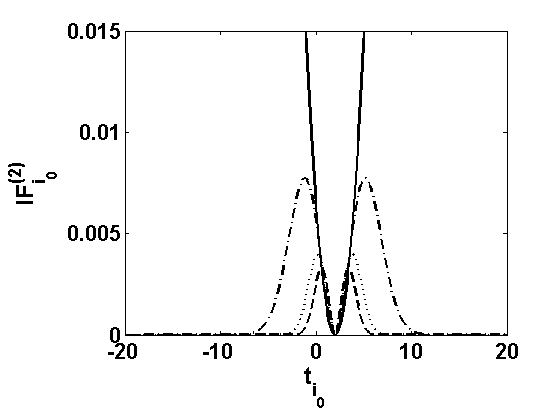
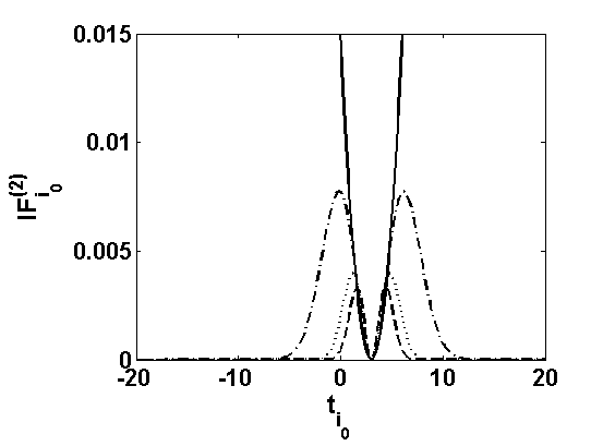
Refer to caption
(a) Design 1, i0=10subscript𝑖010i_{0}=10
Refer to caption
(b) Design 1, i0=40subscript𝑖040i_{0}=40
Refer to caption
(c) Design 1, all directions
Refer to caption
(d) Design 2, i0=10subscript𝑖010i_{0}=10
Refer to caption
(e) Design 2, i0=40subscript𝑖040i_{0}=40
Refer to caption
(f) Design 2, all directions
Refer to caption
(g) Design 3, i0=10subscript𝑖010i_{0}=10
Refer to caption
(h) Design 3, i0=40subscript𝑖040i_{0}=40
Refer to caption
(i) Design 3, all directions
Refer to caption
(j) Design 4, i0=10subscript𝑖010i_{0}=10
Refer to caption
(k) Design 4, i0=40subscript𝑖040i_{0}=40
Refer to caption
(l) Design 4, all directions
Figure 1: Second order influence function of the proposed Wald-type test statistics for testing (50) under the normal regression model with fixed designs 1 – 4 and contamination in the direction i0=10,40subscript𝑖01040i_{0}=10,40 or in all directions at 𝒕=t𝟏𝒕𝑡1\boldsymbol{t}=t\boldsymbol{1} [solid line: τ=0𝜏0\tau=0; dash-dotted line: τ=0.1𝜏0.1\tau=0.1; dotted line: τ=0.3𝜏0.3\tau=0.3; dashed line: τ=0.5𝜏0.5\tau=0.5].                                                                      indicates that the values for τ=0𝜏0\tau=0 (solid line) has been shown in multiple of 102superscript10210^{-2} for this graph only.
Design 1:𝒙i=(1,xi1)T;xi1=a,i=1,,n/2;xi1=b,i=n/2+1,,n.(two-point design)Design 2:𝒙i=(1,xi1)T;xi1,i=1,,n,are pre-fixed iid observations from N(μx,σx2).(Fixed-Normal design)Design 3:𝒙i=(1,xi1)T;xi1=ifori=1,,n.(Divergent design)Design 4:𝒙i=(1,xi1,xi2)T;xi1=1i,xi2=1i2fori=1,,n.(Convergent design)Design 1:formulae-sequencesubscript𝒙𝑖superscript1subscript𝑥𝑖1𝑇formulae-sequencesubscript𝑥𝑖1𝑎formulae-sequence𝑖1𝑛2formulae-sequencesubscript𝑥𝑖1𝑏𝑖𝑛21𝑛(two-point design)Design 2:formulae-sequencesubscript𝒙𝑖superscript1subscript𝑥𝑖1𝑇subscript𝑥𝑖1𝑖1𝑛are pre-fixed iid observations from 𝑁subscript𝜇𝑥superscriptsubscript𝜎𝑥2(Fixed-Normal design)Design 3:formulae-sequenceformulae-sequencesubscript𝒙𝑖superscript1subscript𝑥𝑖1𝑇subscript𝑥𝑖1𝑖for𝑖1𝑛(Divergent design)Design 4:formulae-sequenceformulae-sequencesubscript𝒙𝑖superscript1subscript𝑥𝑖1subscript𝑥𝑖2𝑇formulae-sequencesubscript𝑥𝑖11𝑖subscript𝑥𝑖21superscript𝑖2for𝑖1𝑛(Convergent design)\begin{array}[]{lll}\mbox{Design 1:}&\boldsymbol{x}_{i}=(1,x_{i1})^{T};~{}~{}x_{i1}=a,i=1,\ldots,n/2;x_{i1}=b,i=n/2+1,\ldots,n.&\mbox{(two-point design)}\\ \mbox{Design 2:}&\boldsymbol{x}_{i}=(1,x_{i1})^{T};~{}~{}{x}_{i1},i=1,\ldots,n,\mbox{are pre-fixed iid observations from }N(\mu_{x},\sigma_{x}^{2}).&\mbox{(Fixed-Normal design)}\\ \mbox{Design 3:}&\boldsymbol{x}_{i}=(1,x_{i1})^{T};~{}~{}x_{i1}=i~{}\mbox{for}~{}i=1,\ldots,n.&\mbox{(Divergent design)}\\ \mbox{Design 4:}&\boldsymbol{x}_{i}=(1,x_{i1},x_{i2})^{T};~{}~{}x_{i1}=\frac{1}{i},~{}x_{i2}=\frac{1}{i^{2}}~{}\mbox{for}~{}i=1,\ldots,n.&\mbox{(Convergent design)}\end{array}

Note that, the 𝑪xsubscript𝑪𝑥\boldsymbol{C}_{x} matrix is finitely defined and is positive definite for the first two designs with values

𝑪x=(112(a+b)12(a+b)12(a2+b2))and𝑪x=(1μxμxσx2+μx2)subscript𝑪𝑥matrix112𝑎𝑏12𝑎𝑏12superscript𝑎2superscript𝑏2andsubscript𝑪𝑥matrix1subscript𝜇𝑥subscript𝜇𝑥superscriptsubscript𝜎𝑥2superscriptsubscript𝜇𝑥2\boldsymbol{C}_{x}=\begin{pmatrix}\begin{array}[]{cc}1&\frac{1}{2}(a+b)\\ \frac{1}{2}(a+b)&\frac{1}{2}(a^{2}+b^{2})\end{array}\end{pmatrix}~{}~{}\mbox{and}~{}~{}\boldsymbol{C}_{x}=\begin{pmatrix}\begin{array}[]{cc}1&\mu_{x}\\ \mu_{x}&\sigma_{x}^{2}+\mu_{x}^{2}\end{array}\end{pmatrix}

respectively. In our illustrations, we have taken a=1𝑎1a=1, b=2𝑏2b=2 in design 1 and μx=0subscript𝜇𝑥0\mu_{x}=0, σx=1subscript𝜎𝑥1\sigma_{x}=1 in Design 2 so that the first one is asymmetric and non-orthogonal but the second one is symmetric and orthogonal. The design matrix for Designs 3 and 4 are positive definite for any finite sample sizes, but the corresponding 𝑪xsubscript𝑪𝑥\boldsymbol{C}_{x} matrices have all elements except their (1,1)11(1,1)-th element as \infty and 00 respectively; however, for the computation of the above fixed sample IFs in these cases we can use the finite sample approximation of 𝑪xsubscript𝑪𝑥\boldsymbol{C}_{x} by 1n(𝑿T𝑿)1𝑛superscript𝑿𝑇𝑿\frac{1}{n}(\boldsymbol{X}^{T}\boldsymbol{X}). Figure 1 presents the second order IF of our test statistics for different contamination direction under these four designs at the finite sample size n=50𝑛50n=50 with 𝜷0=𝟏subscript𝜷01\boldsymbol{\beta}_{0}=\boldsymbol{1}, the vector of ones, ϕ0=1subscriptitalic-ϕ01\phi_{0}=1 and different values of τ𝜏\tau. The boundedness of these IFs at τ>0𝜏0\tau>0 clearly indicates the robustness of our proposed Wald-type tests. Further, the (absolute) supremum of these IFs also decreases as τ𝜏\tau increases which implies the increasing robustness of the proposal with increasing τ𝜏\tau. The extent of this increase in robustness for τ>0𝜏0\tau>0 over τ=0𝜏0\tau=0 becomes more prominent when contamination is in all directions and/or the size of the fixed design matrix increases (an extreme increment is in the case of Figure 3i).

Noting that the LIF is always zero, we can next study the power influence function also. In the present case, the PIF can be seen to have the form

PIF(𝐭;Wn,𝐅¯𝜽0)𝑃𝐼𝐹𝐭subscript𝑊𝑛subscript¯𝐅subscript𝜽0\displaystyle PIF(\mathbf{t};W_{n},\mathbf{\underline{F}}_{{\boldsymbol{\theta}}_{0}}) =\displaystyle= Kk(δ)2ϕ0(1+2τ)3/2(1+τ)3/2i=1n(ti𝒙iT𝜷0)eτ(ti𝒙iT𝜷0)22ϕ0[𝒅T𝑪x(𝑿T𝑿)1𝒙i],superscriptsubscript𝐾𝑘𝛿2subscriptitalic-ϕ0superscript12𝜏32superscript1𝜏32superscriptsubscript𝑖1𝑛subscript𝑡𝑖superscriptsubscript𝒙𝑖𝑇subscript𝜷0superscript𝑒𝜏superscriptsubscript𝑡𝑖superscriptsubscript𝒙𝑖𝑇subscript𝜷022subscriptitalic-ϕ0delimited-[]superscript𝒅𝑇subscript𝑪𝑥superscriptsuperscript𝑿𝑇𝑿1subscript𝒙𝑖\displaystyle K_{k}^{\ast}\left(\delta\right)\frac{2}{\phi_{0}}(1+2\tau)^{3/2}(1+\tau)^{-3/2}\sum_{i=1}^{n}\left(t_{i}-\boldsymbol{x}_{i}^{T}\boldsymbol{\beta}_{0}\right)e^{-\frac{\tau\left(t_{i}-\boldsymbol{x}_{i}^{T}\boldsymbol{\beta}_{0}\right)^{2}}{2\phi_{0}}}\left[\boldsymbol{d}^{T}\boldsymbol{C}_{x}(\boldsymbol{X}^{T}\boldsymbol{X})^{-1}\boldsymbol{x}_{i}\right],

where δ𝛿\delta is as given by Equation (53). Figure 2 presents these PIFs for the above four designs with different τ𝜏\tau at the finite sample size n=50𝑛50n=50 with 𝜷0=𝟏subscript𝜷01\boldsymbol{\beta}_{0}=\boldsymbol{1}, ϕ0=1subscriptitalic-ϕ01\phi_{0}=1, 𝒅=102𝜷𝒅superscript102𝜷\boldsymbol{d}=10^{-2}\boldsymbol{\beta} and 5%percent55\% level of significance. Again, the power of the proposed Wald-type tests under the normal model seems to be robust for all τ>0𝜏0\tau>0 and for all the fixed designs over the classical non-robust choice of τ=0𝜏0\tau=0. Further, the extent of robustness increases as τ𝜏\tau increases or the size of the design matrix decreases.
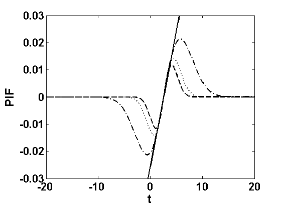
Refer to caption
(a) Design 1
Refer to caption
(b) Design 2
Refer to caption
(c) Design 3
Refer to caption
(d) Design 4
Figure 2: Power influence function of the proposed Wald-type test statistics for testing (50) under the normal regression model with fixed designs 1 – 4 at contamination point 𝒕=t𝟏𝒕𝑡1\boldsymbol{t}=t\boldsymbol{1} [solid line: τ=0𝜏0\tau=0; dash-dotted line: τ=0.1𝜏0.1\tau=0.1; dotted line: τ=0.3𝜏0.3\tau=0.3; dashed line: τ=0.5𝜏0.5\tau=0.5].

5.2 Testing for individual regression coefficients in Poisson model for Count Data

Let us consider another popular special class of GLM applicable to the analysis of count responses, namely the Poisson regression model. Here the response yisubscript𝑦𝑖y_{i} is assumed to have a Poisson distribution with mean e𝒙iT𝜷superscript𝑒superscriptsubscript𝒙𝑖𝑇𝜷e^{\boldsymbol{x}_{i}^{T}\boldsymbol{\beta}} depending on the given predictor values 𝒙isubscript𝒙𝑖\boldsymbol{x}_{i}. In terms of the GLM notations of Section 4, the density in (40) is then a Poisson density with ηi=𝒙iT𝜷subscript𝜂𝑖superscriptsubscript𝒙𝑖𝑇𝜷\eta_{i}=\boldsymbol{x}_{i}^{T}\boldsymbol{\beta}, known ϕ=1italic-ϕ1\phi=1 and the logarithmic link function. So, we can obtain the robust MDPDE 𝜽^τ=𝜷^τsubscript^𝜽𝜏subscript^𝜷𝜏\widehat{\boldsymbol{\theta}}_{\tau}=\widehat{\boldsymbol{\beta}}_{\tau} of the regression parameter 𝜽=𝜷𝜽𝜷\boldsymbol{\theta}=\boldsymbol{\beta} in this case following the general theory of Section 4. Ghosh and Basu (2016) studied these MDPDEs 𝜷^τsubscript^𝜷𝜏\widehat{\boldsymbol{\beta}}_{\tau} under the fixed-design Poisson regression model and their properties in detail with examples. In particular, in the notations of Section 4, we have estimating equations given only by (41) with K1(yi,𝒙iT𝜷,ϕ)=(yi𝒙iT𝜷)subscript𝐾1subscript𝑦𝑖superscriptsubscript𝒙𝑖𝑇𝜷italic-ϕsubscript𝑦𝑖superscriptsubscript𝒙𝑖𝑇𝜷K_{1}(y_{i},\boldsymbol{x}_{i}^{T}\boldsymbol{\beta},\phi)=\left(y_{i}-\boldsymbol{x}_{i}^{T}\boldsymbol{\beta}\right), and the required asymptotic variance matrix 𝚺τsubscript𝚺𝜏\boldsymbol{\Sigma}_{\tau} can be obtained in terms of 𝛀n,τsubscript𝛀𝑛𝜏\boldsymbol{\Omega}_{n,\tau} and 𝚿n,τsubscript𝚿𝑛𝜏\boldsymbol{\Psi}_{n,\tau} as defined in (44).

Here, as our second illustration of the proposed Wald-type testing procedures, we will consider the problem of testing for the significance of any predictor (say, hh-th predictor) in the model. For a fixed integer hh between 1 to k𝑘k, the corresponding hypothesis is given by

H0:βh=0 versus H1:βh0,:subscript𝐻0subscript𝛽0 versus subscript𝐻1:subscript𝛽0H_{0}:\beta_{h}=0\text{ versus }H_{1}:{\beta_{h}}\neq 0, (54)

where βhsubscript𝛽\beta_{h} denotes the hh-th component of the regression vector β𝛽\beta. Clearly this important hypothesis in (54) is a special case of the general linear hypotheses in (45) with r=1𝑟1r=1, 𝑳Tsuperscript𝑳𝑇\boldsymbol{L}^{T} being an k𝑘k-vector with all entries zero except the hh-th entry as 1 and l0=0subscript𝑙00{l}_{0}=0. So, our proposed Wald-type test statistics for this problem, following the general theory of Section 4, can be simplified as

Wn(𝜷^τ)=nβ^h,τ2σhh,τ2(𝜷^τ),subscript𝑊𝑛subscript^𝜷𝜏𝑛superscriptsubscript^𝛽𝜏2superscriptsubscript𝜎𝜏2subscript^𝜷𝜏W_{n}(\widehat{\boldsymbol{\beta}}_{\tau})=\frac{n\widehat{{\beta}}_{h,\tau}^{2}}{\sigma_{hh,\tau}^{2}(\widehat{\boldsymbol{\beta}}_{\tau})}, (55)

where β^h,τsubscript^𝛽𝜏\widehat{{\beta}}_{h,\tau} is the hh-th entry of 𝜷^τsubscript^𝜷𝜏\widehat{\boldsymbol{\beta}}_{\tau} denoting the MDPDE of βhsubscript𝛽\beta_{h} and σhh,τ2subscriptsuperscript𝜎2𝜏\sigma^{2}_{hh,\tau} denote the hh-th diagonal element of the asymptotic covariance matrix 𝚺τsubscript𝚺𝜏\boldsymbol{\Sigma}_{\tau} at the null parameter values denoting the null asymptotic variance of nβ^h,τ𝑛subscript^𝛽𝜏\sqrt{n}\widehat{{\beta}}_{h,\tau}. Following Section 4, this test statistics in (55) is asymptotically distributed as χ12superscriptsubscript𝜒12\chi_{1}^{2} distribution and consistent at any fixed alternatives. Further, denoting the null parameter value as 𝜷0subscript𝜷0\boldsymbol{\beta}_{0} having hh-th entry βh,0=0subscript𝛽00\beta_{h,0}=0, the asymptotic distribution of the proposed Wald-type test statistics under the contiguous alternatives

H1,n:𝜷nwithβh,n=n1/2d,βl,n=βl,0forlh,d{0}H_{1,n}:\boldsymbol{\beta}_{n}~{}\mbox{with}~{}\beta_{h,n}=n^{-1/2}d,\beta_{l,n}=\beta_{l,0}~{}\mbox{for}~{}l\neq h,d\in\mathbb{R}-\{{0}\}

is a non-central χ2superscript𝜒2\chi^{2} distribution with one degree of freedom and non-centrality parameter

δ=d2σhh,τ2(𝜷0).𝛿superscript𝑑2superscriptsubscript𝜎𝜏2subscript𝜷0\delta=\frac{d^{2}}{\sigma_{hh,\tau}^{2}({\boldsymbol{\beta}}_{0})}. (56)

Note that σhh,τ2(𝜷0)superscriptsubscript𝜎𝜏2subscript𝜷0\sigma_{hh,\tau}^{2}({\boldsymbol{\beta}}_{0}) has no closed form expression in this case but can be estimated numerically for any fixed sample size and any given design-matrix by σ^hh,τ2(𝜷0)superscriptsubscript^𝜎𝜏2subscript𝜷0\widehat{\sigma}_{hh,\tau}^{2}({\boldsymbol{\beta}}_{0}), the hh-th diagonal entry of the matrix

𝚿n,τ1(𝜷0)𝛀n,τ(𝜷0)𝚿n,τ1(𝜷0)superscriptsubscript𝚿𝑛𝜏1subscript𝜷0subscript𝛀𝑛𝜏subscript𝜷0superscriptsubscript𝚿𝑛𝜏1subscript𝜷0\boldsymbol{\Psi}_{n,\tau}^{-1}({\boldsymbol{\beta}}_{0})\boldsymbol{\Omega}_{n,\tau}({\boldsymbol{\beta}}_{0})\boldsymbol{\Psi}_{n,\tau}^{-1}({\boldsymbol{\beta}}_{0})

estimating 𝚺τ(𝜷0)subscript𝚺𝜏subscript𝜷0\boldsymbol{\Sigma}_{\tau}({\boldsymbol{\beta}}_{0}). Therefore, the effect of given design points can not be separated out explicitly from the form of asymptotic contiguous power based on this non-central distribution as was the case for previous normal model. We again consider the four given designs 1–4 from Section 5.1 and numerically compute the asymptotic contiguous power of the proposed Wald-type tests for testing (54) with different values of hh, d𝑑d and τ𝜏\tau assuming n=50𝑛50n=50, βl,0=1subscript𝛽𝑙01\beta_{l,0}=1 for all lh𝑙l\neq h and 5%percent55\% level of significance; the results are shown in Table 2. Once again, the power loss is not quite significant for any small positive values of τ𝜏\tau. Also, we need larger values of d𝑑d to attain any fixed power by the proposed Wald-type test statistics with fixed tuning parameter whenever the values of the fixed design variables increases.

Table 2: Contiguous power of the proposed Wald-type test for testing (54) under the Poisson regression model
Design τ𝜏\tau τ𝜏\tau
dxsubscript𝑑𝑥d_{x} 0 0.1 0.3 0.5 0.7 1 0 0.1 0.3 0.5 0.7 1
Design 1 h=11h=1 h=22h=2
0 0.050 0.050 0.050 0.050 0.050 0.050 0.050 0.050 0.050 0.050 0.050 0.050
2 0.200 0.199 0.189 0.178 0.167 0.152 0.378 0.375 0.355 0.331 0.308 0.276
3 0.388 0.383 0.364 0.339 0.315 0.282 0.696 0.691 0.663 0.627 0.589 0.534
5 0.796 0.792 0.766 0.730 0.692 0.634 0.985 0.984 0.978 0.968 0.954 0.926
7 0.974 0.973 0.964 0.950 0.932 0.897 1.000 1.000 1.000 1.000 0.999 0.998
10 1.000 1.000 1.000 0.999 0.999 0.996 1.000 1.000 1.000 1.000 1.000 1.000
Design 2 h=11h=1 h=22h=2
0 0.050 0.050 0.050 0.050 0.050 0.050 0.050 0.050 0.050 0.050 0.050 0.050
1 0.140 0.139 0.132 0.124 0.117 0.110 0.320 0.316 0.300 0.280 0.261 0.234
2 0.414 0.408 0.381 0.351 0.326 0.299 0.846 0.842 0.819 0.786 0.749 0.693
3 0.743 0.735 0.700 0.658 0.619 0.574 0.994 0.994 0.991 0.985 0.977 0.959
5 0.992 0.991 0.985 0.976 0.965 0.947 1.000 1.000 1.000 1.000 1.000 1.000
7 1.000 1.000 1.000 1.000 1.000 0.999 1.000 1.000 1.000 1.000 1.000 1.000
Design 3 h=11h=1 h=22h=2
0 0.050 0.050 0.050 0.050 0.050 0.050 0.050 0.050 0.050 0.050 0.050 0.050
0.01 1.000 1.000 1.000 1.000 1.000 1.000 0.057 0.056 0.056 0.056 0.055 0.055
0.05 1.000 1.000 1.000 1.000 1.000 1.000 0.221 0.219 0.209 0.196 0.183 0.166
0.1 1.000 1.000 1.000 1.000 1.000 1.000 0.662 0.657 0.630 0.593 0.557 0.503
0.2 1.000 1.000 1.000 1.000 1.000 1.000 0.997 0.997 0.996 0.993 0.988 0.976
0.5 1.000 1.000 1.000 1.000 1.000 1.000 1.000 1.000 1.000 1.000 1.000 1.000
Design 4 h=22h=2 h=33h=3
0 0.050 0.050 0.050 0.050 0.050 0.050 0.050 0.050 0.050 0.050 0.050 0.050
10 0.153 0.152 0.145 0.137 0.129 0.119 0.168 0.167 0.159 0.149 0.140 0.128
20 0.459 0.455 0.431 0.402 0.373 0.333 0.510 0.506 0.479 0.445 0.412 0.366
30 0.795 0.792 0.765 0.728 0.689 0.630 0.845 0.841 0.816 0.781 0.740 0.679
50 0.996 0.996 0.994 0.990 0.983 0.968 0.999 0.999 0.998 0.995 0.992 0.981
70 1.000 1.000 1.000 1.000 1.000 1.000 1.000 1.000 1.000 1.000 1.000 1.000
Refer to caption
(a) Design 1, i0=10subscript𝑖010i_{0}=10
Refer to caption
(b) Design 1, i0=40subscript𝑖040i_{0}=40
Refer to caption
(c) Design 1, all directions
Refer to caption
(d) Design 2, i0=10subscript𝑖010i_{0}=10
Refer to caption
(e) Design 2, i0=40subscript𝑖040i_{0}=40
Refer to caption
(f) Design 2, all directions
Refer to caption
(g) Design 3, i0=10subscript𝑖010i_{0}=10
Refer to caption
(h) Design 3, i0=40subscript𝑖040i_{0}=40
Refer to caption
(i) Design 3, all directions
Refer to caption
(j) Design 4, i0=10subscript𝑖010i_{0}=10
Refer to caption
(k) Design 4, i0=40subscript𝑖040i_{0}=40
Refer to caption
(l) Design 4, all directions
Figure 3: Second order influence function of the proposed Wald-type test statistics for testing (54) under Poisson regression model with fixed designs 1 – 4 and contamination in the direction i0=10,40subscript𝑖01040i_{0}=10,40 or in all directions at 𝒕=t𝟏𝒕𝑡1\boldsymbol{t}=t\boldsymbol{1} [solid line: τ=0𝜏0\tau=0; dash-dotted line: τ=0.1𝜏0.1\tau=0.1; dotted line: τ=0.3𝜏0.3\tau=0.3; dashed line: τ=0.5𝜏0.5\tau=0.5].

Further, the robustness of our proposed Wald-type tests can also be verified by examining the second order influence function of the test statistics and the power influence functions from their general expressions derived in Section 4. However, in the present case of Poisson regression model, we cannot have more simplified explicit expressions for them except for the particular form of K1(yi,𝒙iT𝜷,ϕ)subscript𝐾1subscript𝑦𝑖superscriptsubscript𝒙𝑖𝑇𝜷italic-ϕK_{1}(y_{i},\boldsymbol{x}_{i}^{T}\boldsymbol{\beta},\phi) as defined above and no K2(yi,𝒙iT𝜷,ϕ)subscript𝐾2subscript𝑦𝑖superscriptsubscript𝒙𝑖𝑇𝜷italic-ϕK_{2}(y_{i},\boldsymbol{x}_{i}^{T}\boldsymbol{\beta},\phi); but they can be easily computed numerically for any given fixed design. We again present the numerical values of the second order influence functions of the proposed Wald-type test statistics for testing significance of the first slope parameter β2subscript𝛽2\beta_{2} (h=22h=2 in (54)) at different values of τ𝜏\tau under the four designs considered in Section 5.1 with n=50𝑛50n=50 and βl,0=1subscript𝛽𝑙01\beta_{l,0}=1 for all l2𝑙2l\neq 2; these are presented in Figures 3. The redescending nature of all the influence functions with increasing τ𝜏\tau is again quite clear from the figures, which indicates the increasing robustness of our proposed Wald-types tests as τ>0𝜏0\tau>0 increases over the non-robust choice τ=0𝜏0\tau=0 (having unbounded IFs). The nature of the power influence functions in this case are also seen to be very similar implying the robustness of our proposal at τ>0𝜏0\tau>0; so we skip them for brevity.

6 Concluding remarks and the Choice of τ𝜏\tau

We have proposed a robust parametric hypothesis testing approach for general non-homogeneous observations involving a common model parameter. The test statistics have been constructed by generalizing the Wald test statistics using the robust minimum density power divergence estimator (with parameter τ0𝜏0\tau\geq 0) of the underlying common parameter in place of its non-robust maximum likelihood estimator. The properties of the proposed test have been studied for both simple and composite hypotheses under general non-homogeneous set-up and applied to the cases of several fixed design GLMs. In particular, it has been observed that the proposed tests have simple chi-square asymptotic limit under null hypothesis in contrast to the linear combination of chi-square limit for the robust tests of Ghosh and Basu (2017) making its application much easier under complex models. Also, the tests are always consistent at any fixed alternatives and have bounded second order influence functions of the test statistics and bounded power influence functions for τ>0𝜏0\tau>0 implying robustness of our proposal.

Further, in each of the examples considered, we have seen that the asymptotic power of the proposed Wald-type tests under any contiguous alternatives as well as the extent of robustness depends on the tuning parameter τ𝜏\tau. In particular, as τ𝜏\tau increases, the contiguous power decreases slightly from its highest value at τ=0𝜏0\tau=0 corresponding to the non-robust classical MLE based Wald test but the robustness increases significantly. Thus, the tuning parameter τ𝜏\tau yields a trade-off between asymptotic contiguous power and robustness of these Wald-type tests; note the similarity with the trade-off between asymptotic efficiency and robustness of the underlying MDPDE as studied in Ghosh and Basu (2013). In fact one can explicitly examine, from the theoretical results derived here, that the dependence of the power and robustness of the proposed Wald-type tests comes directly through the similar dependence of the efficiency and robustness of the MDPDE used in constructing the test statistics. Hence a proper choice of the tuning parameter τ𝜏\tau balancing the asymptotic power and robustness can be equivalently obtained by balancing the corresponding trade-off for the underlying MDPDE. This latter problem under the non-homogeneous set-up has been proposed and studied by Ghosh and Basu (2013, 2015, 2016), where it is proposed that a data-driven estimate of the mean square error of the MDPDE be minimized to obtain the optimum tuning parameter for any given practical dataset. The same optimum τ𝜏\tau can also be used as well for applying our proposed Wald-type tests for any practical hypothesis testing problems. However, more detailed investigation on this issue could ba an interesting future research work.

Another possible future extension of the present paper will be to construct similar robust testing procedures for two independent samples of non-homogeneous data. This problem is of high practical relevance as one can then use the construction to test between two regression lines from fixed design clinical trials occurring frequently in medical sciences and epidemiology. The corresponding problem with homogeneous sample has been recently tackled by Ghosh et al. (2017) which should be extended to the cases with non-homogeneous data and fixed-design regressions as in the present paper. We hope to pursue some such extensions in future.

Appendix A Assumptions

Assumptions required for Asymptotic distributions of the MDPDE under non-homogeneous data (Ghosh and Basu, 2013):

  1. (A1)

    For all i=1,,n𝑖1𝑛i=1,\ldots,n, the support of model distribution given by χ={y|fi,𝜽(y)>0}𝜒conditional-set𝑦subscript𝑓𝑖𝜽𝑦0\chi=\{y|f_{i,\boldsymbol{\theta}}(y)>0\} is independent of i𝑖i and 𝜽𝜽\boldsymbol{\theta} and is the same as the support of true distribution Gisubscript𝐺𝑖G_{i} for each i𝑖i.

  2. (A2)

    There exists an open subset ωΘ𝜔Θ\omega\subseteq\Theta that contains the best fitting parameter 𝜽g=𝑻τ(𝑮¯)superscript𝜽𝑔subscript𝑻𝜏¯𝑮\boldsymbol{\theta}^{g}=\boldsymbol{T}_{\tau}(\underline{\boldsymbol{G}}) and, at each 𝜽ω𝜽𝜔\boldsymbol{\theta}\in\omega, the model density fi,𝜽(y)subscript𝑓𝑖𝜽𝑦f_{i,\boldsymbol{\theta}}(y) is thrice continuously differentiable with respect to θ𝜃\theta for almost all yχ𝑦𝜒y\in\chi and all i=1,,n𝑖1𝑛i=1,\ldots,n.

  3. (A3)

    fi,𝜽(y)1+α𝑑ysubscript𝑓𝑖𝜽superscript𝑦1𝛼differential-d𝑦\int f_{i,\boldsymbol{\theta}}(y)^{1+\alpha}dy and fi,𝜽(y)αgi(y)𝑑ysubscript𝑓𝑖𝜽superscript𝑦𝛼subscript𝑔𝑖𝑦differential-d𝑦\int f_{i,\boldsymbol{\theta}}(y)^{\alpha}g_{i}(y)dy can be differentiated three times with respect to θ𝜃\theta, and the derivatives can be taken under the integral sign for any i=1,,n𝑖1𝑛i=1,\ldots,n.

  4. (A4)

    The matrix 𝑱i,τsubscript𝑱𝑖𝜏\boldsymbol{J}_{i,\tau} is positive definite for any i=1,,n𝑖1𝑛i=1,\ldots,n, and, infn[mineigenvalue of 𝚿n,τ]>0.subscriptinfimum𝑛delimited-[]eigenvalue of subscript𝚿𝑛𝜏0\displaystyle\inf_{n}[\min~{}\mbox{eigenvalue of }\boldsymbol{\Psi}_{n,\tau}]>0.

  5. (A5)

    Define Vi,𝜽(y)=[fi,𝜽(y)1+α𝑑y(1+1α)fi,𝜽(y)α]subscript𝑉𝑖𝜽𝑦delimited-[]subscript𝑓𝑖𝜽superscript𝑦1𝛼differential-d𝑦11𝛼subscript𝑓𝑖𝜽superscript𝑦𝛼V_{i,\boldsymbol{\theta}}(y)=\left[\int f_{i,\boldsymbol{\theta}}(y)^{1+\alpha}dy-\left(1+\frac{1}{\alpha}\right)f_{i,\boldsymbol{\theta}}(y)^{\alpha}\right]. For all 𝜽Θ𝜽Θ\boldsymbol{\theta}\in\Theta, i=1,,n𝑖1𝑛i=1,\ldots,n, and all j,h,l=1,,kformulae-sequence𝑗𝑙1𝑘j,h,l=1,\ldots,k, the (j,h,l)𝑗𝑙(j,h,l)-th (third order) partial derivatives of Vi,𝜽(y)subscript𝑉𝑖𝜽𝑦V_{i,\boldsymbol{\theta}}(y) is bounded in absolute value by some functions Mjhl(i)(y)superscriptsubscript𝑀𝑗𝑙𝑖𝑦M_{jhl}^{(i)}(y) satisfying 1ni=1nEgi[Mjhl(i)(Y)]=O(1)1𝑛superscriptsubscript𝑖1𝑛subscript𝐸subscript𝑔𝑖delimited-[]superscriptsubscript𝑀𝑗𝑙𝑖𝑌𝑂1\displaystyle\frac{1}{n}\sum_{i=1}^{n}E_{g_{i}}\left[M_{jhl}^{(i)}(Y)\right]=O(1).

  6. (A6)

    For all j,h=1,,kformulae-sequence𝑗1𝑘j,h=1,\ldots,k, define 𝑵ijh(1)(y)=jVi,𝜽(y)superscriptsubscript𝑵𝑖𝑗1𝑦subscript𝑗subscript𝑉𝑖𝜽𝑦\boldsymbol{N}_{ijh}^{(1)}(y)=\nabla_{j}V_{i,\boldsymbol{\theta}}(y) and 𝑵ijh(2)(y)=jhVi,𝜽(y)Egi(jhVi,𝜽(y))superscriptsubscript𝑵𝑖𝑗2𝑦subscript𝑗subscript𝑉𝑖𝜽𝑦subscript𝐸subscript𝑔𝑖subscript𝑗subscript𝑉𝑖𝜽𝑦\boldsymbol{N}_{ijh}^{(2)}(y)=\nabla_{jh}V_{i,\boldsymbol{\theta}}(y)-E_{g_{i}}(\nabla_{jh}V_{i,\boldsymbol{\theta}}(y)). Then, we have

    limNsupn>1{1ni=1nEgi|𝑵ijh(l)(y)|I(|𝑵ijh(l)(y))|>N)}=0,l=1,2.\displaystyle\lim_{N\rightarrow\infty}\sup_{n>1}\Biggl{\{}\frac{1}{n}\sum_{i=1}^{n}E_{g_{i}}|\boldsymbol{N}_{ijh}^{(l)}(y)|I(|\boldsymbol{N}_{ijh}^{(l)}(y))|>N)\Biggr{\}}=0,~{}~{}l=1,2.
  7. (A7)

    For any ϵ>0italic-ϵ0\epsilon>0,

    limn{1ni=1nEgi[𝛀n1/2Vi,𝜽(y)2I(𝛀n1/2Vi,𝜽(y)>ϵn)]}=0.subscript𝑛1𝑛superscriptsubscript𝑖1𝑛subscript𝐸subscript𝑔𝑖delimited-[]superscriptnormsuperscriptsubscript𝛀𝑛12subscript𝑉𝑖𝜽𝑦2𝐼normsuperscriptsubscript𝛀𝑛12subscript𝑉𝑖𝜽𝑦italic-ϵ𝑛0\lim_{n\rightarrow\infty}\left\{\frac{1}{n}\sum_{i=1}^{n}E_{g_{i}}\left[||\boldsymbol{\Omega}_{n}^{-1/2}\nabla V_{i,\boldsymbol{\theta}}(y)||^{2}I(||\boldsymbol{\Omega}_{n}^{-1/2}\nabla V_{i,\boldsymbol{\theta}}(y)||>\epsilon\sqrt{n})\right]\right\}=0. (57)

Assumptions required for Asymptotic distributions of the MDPDE under Normal Fixed-Design Linear Model (Ghosh and Basu, 2013):
The values of given design point 𝒙i=(x1i,,xki)Tsubscript𝒙𝑖superscriptsubscript𝑥1𝑖subscript𝑥𝑘𝑖𝑇\boldsymbol{x}_{i}=(x_{1i},\ldots,x_{ki})^{T} are such that

  1. (R1)

    supn>1max1in|xji|=O(1)subscriptsupremum𝑛1subscript1𝑖𝑛subscript𝑥𝑗𝑖𝑂1\displaystyle\sup_{n>1}\max_{1\leq i\leq n}~{}|x_{ji}|=O(1), supn>1max1in|xjixli|=O(1)subscriptsupremum𝑛1subscript1𝑖𝑛subscript𝑥𝑗𝑖subscript𝑥𝑙𝑖𝑂1\displaystyle\sup_{n>1}\max_{1\leq i\leq n}~{}|x_{ji}x_{li}|=O(1), and 1ni=1n|xjixlixhi|=O(1)1𝑛superscriptsubscript𝑖1𝑛subscript𝑥𝑗𝑖subscript𝑥𝑙𝑖subscript𝑥𝑖𝑂1\displaystyle\frac{1}{n}\sum_{i=1}^{n}~{}|x_{ji}x_{li}x_{hi}|=O(1), for all j,l,h=1,,k.formulae-sequence𝑗𝑙1𝑘j,l,h=1,\ldots,k.

  2. (R2)

    infn[mineigenvalue of 1n(𝑿T𝑿)]>0.subscriptinfimum𝑛delimited-[]eigenvalue of 1𝑛superscript𝑿𝑇𝑿0\displaystyle\inf_{n}\left[\min~{}\mbox{eigenvalue of }\frac{1}{n}(\boldsymbol{X}^{T}\boldsymbol{X})\right]>0.

References

  • Aerts and Haesbroeck (2016) Aerts, S. and Haesbroeck, G. (2016). Robust asymptotic tests for the equality of multivariate coefficients of variation Test, doi: 10.1007/s11749-016-0504-4.
  • Basu et al. (1998) Basu, A., Harris, I. R., Hjort, N. L., and Jones, M. C. (1998). Robust and efficient estimation by minimising a density power divergence. Biometrika, 85, 549–559.
  • Basu et al. (2011) Basu, A., Shioya, H. and Park, C. (2011). Statistical Inference: The Minimum Distance Approach. Chapman &\& Hall/CRC, Boca de Raton.
  • Basu et al. (2016) Basu, A., Mandal, A., Martin, N. and Pardo, L. (2016) Generalized Wald-type tests based on minimum density power divergence estimators. Statistics, 50(1), 1–26.
  • Basu et al. (2017a) Basu, A., Ghosh, A., Mandal, A., Martin, N. and Pardo, L. (2017a) A Wald-type test statistic for testing linear Hypothesis in logistic regression models based on minimum density power divergence estimator. Electronic Journal of Statistics, 11, 2741–2772.
  • Basu et al. (2017b) Basu, A., Ghosh, A., Mandal, A., Martin, N. and Pardo, L. (2017b) Robust Wald-type tests in GLM with random design based on minimum density power divergence estimators. Pre-print.
  • Beran (1982) Beran, R. (1982). Robust estimation in models for independent non-identically distributed data. The Annals of Statistics, 10, 2, 418-428.
  • Cochran (1952) Cochran, W. G. (1952). The χ2superscript𝜒2\chi^{2} test of goodness of fit. Annals of Mathematical Statistics, 23, 15-28.
  • Ghosh and Basu (2013) Ghosh, A., and Basu, A. (2013). Robust estimation for independent non-homogeneous observations using density power divergence with applications to linear regression. Electronic Journal of Statistics, 7, 2420–2456.
  • Ghosh and Basu (2015) Ghosh, A., and Basu, A. (2015). Robust Estimation for Non-Homogeneous Data and the Selection of the Optimal Tuning Parameter: The DPD Approach Journal of Applied Statistics, 42(9), 2056–2072.
  • Ghosh and Basu (2016) Ghosh, A., and Basu, A. (2016). Robust Estimation in Generalized Linear Models : The Density Power Divergence Approach. Test, 25(2), 269–290.
  • Ghosh and Basu (2017) Ghosh, A., and Basu, A. (2017). Robust Bounded Influence Tests for Independent but Non-Homogeneous Observations. Statistica Sinica, doi:10.5705/ss.202015.0320.
  • Ghosh et al. (2015) Ghosh, A., Basu, A., and Pardo, L. (2015). On the robustness of a divergence based test of simple statistical hypotheses. Journal of Statistical Planning and Inference, 116, 91–108.
  • Ghosh et al. (2016) Ghosh, A., Mandal, A., Martin, N. and Pardo, L. (2016). Influence analysis of robust Wald-type tests. Journal of Multivariate Analysis, 147, 102–126.
  • Ghosh et al. (2017) Ghosh, A., Martin, N., Basu, A., and Pardo, L. (2017). A New Class of Robust Two-Sample Wald-Type Tests. ArXiv Pre-print, arXiv:1702.04552 [stat.ME].
  • Hampel et al. (1986) Hampel, F. R., Ronchetti, E., Rousseeuw, P. J., and Stahel W.(1986). Robust Statistics: The Approach Based on Influence Functions. New York, USA: John Wiley & Sons.
  • Heritier and Ronchetti (1994) Heritier, S. and Ronchetti, E. (1994). Robust bounded-influence tests in general parametric models. Journal of the American Statistical Association, 89, 897–904.
  • Huber (1983) Huber, P. J. (1983). Minimax aspects of bounded-influence regression (with discussion). Journal of the American Statistical Association, 69, 383-393.
  • Muller (1998) Muller, C. (1998). Optimum robust testing in linear models. The Annals of Statistics, 26, 3, 1126-1146.
  • Rousseeuw and Ronchetti (1979) Rousseeuw, P. J. and Ronchetti, E. (1979). The influence curve for tests. Research Report 21, Fachgruppe für Statistik, ETH, Zurich.
  • Rousseeuw and Ronchetti (1981) Rousseeuw, P. J. and Ronchetti, E. (1981). Influence curves for general statistics. J. Comput. Appl. Math., 7, 161–166.
  • Toma and Broniatowski (2010) Toma, A. and Broniatowski, M. (2010). Dual divergence estimators and tests: robustness results. Journal of Multivariate Analysis, 102, 20–36.