Pure states in the SYK model
and nearly- gravity
Ioanna Kourkoulou1 and Juan Maldacena2
1Jadwin Hall, Princeton University, Princeton, NJ 08540, USA
2Institute for Advanced Study, Princeton, NJ 08540, USA
We consider pure states in the SYK model. These are given by a simple local condition on the Majorana fermions, evolved over an interval in Euclidean time to project on to low energy states. We find that “diagonal” correlators are exactly the same as thermal correlators at leading orders in the large expansion. We also describe “off diagonal” correlators that decay in time, and are given simply in terms of thermal correlators. We also solved the model numerically for low values of and noticed that subsystems become typically entangled after an interaction time. In addition, we identified configurations in two dimensional nearly- gravity with similar symmetries. These gravity configurations correspond to states with regions behind horizons. The region behind the horizon can be made accessible by modifying the Hamiltonian of the boundary theory using the the knowledge of the particular microstate. The set of microstates in the SYK theory with these properties generates the full Hilbert space.
1 Introduction
The SYK model involves Majorana fermions undergoing few body interactions with random couplings [1, 2]. At low energies, it is a maximally chaotic model that has some features in common with near extremal black holes, or more precisely, with nearly- gravity [3, 2, 4, 5, 6, 7]. In this paper, we consider the evolution of particular pure states in the SYK model. We study some aspects of the thermalization of these states. We also attempt to draw some lessons for the geometry associated to particular microstates for nearly- black holes.
The particular initial pure states are obtained by combining pairs of Majorana fermions into qubit like operators and choosing states with definite eigenvalues for the components of all qubits. By choosing different eigenvalues we get a whole basis of the Hilbert space. We further evolve these states over some distance in Euclidean time in order to get low energy states.
Up to the first few orders in the expansion, one can compute the correlators of this model in terms of finite temperature correlation functions, with . The correlators of fermions with the same index turn out to be the same as thermal correlators. We interpret this as saying that the “gravitational background” for these states is the same as that of the thermal state. Some other correlators, such as correlators involving fermions with different indices, are different from the thermal ones, which are zero for different indices. However, they can still be computed in terms of suitable thermal correlators. These are such that they decay away under Lorentzian evolution, reflecting the thermalization of the system.
The gravity dual of the SYK model is not precisely known. However, at low energies there is an emergent reparametrization symmetry that is both spontaneously and explicitly broken [2]. This pattern of symmetries is also present in nearly- gravity, where the reparametrization symmetry is the asymptotic symmetry of [4, 5, 6, 7]. In the same spirit, we identify some nearly- gravity configurations that have properties similar to the pure states in the SYK model. Namely, we will see that the symmetries are broken in a similar fashion. These pure states have a gravity description which involves again the full space, but we introduce a shockwave at on the left boundary. Correspondingly, in Euclidean space, we continue to have a disk, but with a special point at the boundary. This special point is the source of the shock wave in the Lorentzian geometry. An interesting feature of the geometric configuration is that it contains a region behind the horizon. The shock wave is separated from the horizon. This suggests that we have a whole basis of states in the Hilbert space with a smooth horizon. The region behind the horizon is not accesible to simple experiments by the boundary observer. However, as studied in [8], evolving the system with a modified Hamiltonian we can make some of the region behind the horizon visible. Here, we can make the whole spatial slice visible.
For this purpose he/she has to add a term to the Hamiltonian that depends on the particular microstate that is chosen. The procedure is essentially the same as the one that renders wormholes traversable [9, 10].
This paper is organized as follows. In section two we define the model and define a set of simple initial states. In section three we display the large solution. In section four we discuss some aspects of the low energy limit. In section five we present some numerical diagonalization results, discussing the decay of correlators, the rise of entanglement entropy, and we check statements about the large solution. In section 6 we discuss some aspects of the gravity interpretation. In section 7 we give the protocol for looking behind the horizon for these states. We end with a final discussion.
2 Definition of the model and the initial states
We consider the SYK model [1, 2]. We consider a Hilbert space generated by an even number, , of Majorana fermions , with . It has a Hamiltonian of the form
| (2.1) |
with couplings which are all independent random numbers drawn from a gaussian distribution with variance set by , see [11] for more details. More generally one can also consider a model with a Hamiltonian involving fermions .
We are interested in considering the evolution of special pure states. For example, we can consider the state that obeys the conditions
| (2.2) |
If we imagine and as proportional to the and Pauli matrices, then will have spin minus under . More precisely, we can say that the state has all plus eigenvalues for the operators
| (2.3) |
More generally, we can define a whole set of states by the conditions
| (2.4) |
This defines states, one for each choice of the signs of all the , which form a basis of the Hilbert space.
The SYK evolution with (2.1) will give states which are linear combinations of these states. At long times we expect to get fairly generic linear combinations so that the state becomes effectively thermalized (even though it remains a pure state). If we think of as a simple state were all qubits point up, then the evolution will start flipping some of the qubits so that we start getting a more general superposition of states with qubits pointing up and down111 The SYK evolution does preserve the sign of .. More importantly, we get linear superpositions of such states. The SYK evolution can be viewed as a set of simple quantum gates that acts on the simple state generating a more complex state.
We expect these states, (2.4), to have an energy close to zero for the SYK hamiltonian. These are states of high energy compared to the minimal energy of the SYK model which is of order .
We can produce lower energy states by evolving with the Euclidean Hamiltonian . In this way we can form an overcomplete set of low energy states. We expect that the expansion of is in terms of the energy eigenstates is
| (2.5) |
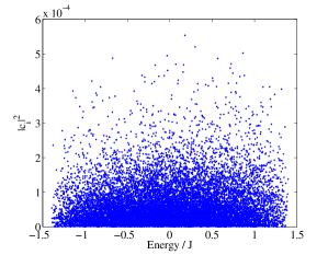
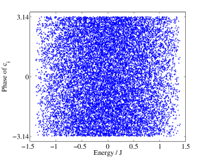
where the typical is of order of 222 Of course, some of the are zero for symmetry reasons. For example, since commutes with the Hamiltonian, all states that appear have to have the same value of as the state . . In figure 2 we see an example for obtained by exact numerical diagonalization.
Note that we can average the correlators over all choices of signs . This reproduces the thermal ensemble exactly,
| (2.6) |
This means that we can view the states as an (overcomplete) basis of the low energy states relevant to the dynamics at temperature . We see that after averaging over all sign choices for the states we get the exact thermal average. Of course, (2.6) is not at all surprising, given the way we have defined the states. What is more interesting is that each individual state gives rise to correlators that look thermal to high accuracy, as we will demonstrate below.
3 The large solution
3.1 Two point functions from thermal ones
In this section we analyze this problem in the large limit. The proper way to treat the average over random couplings is to introduce replicas [11]. However, one finds that (for the replica diagonal solution) the interaction between replicas is down by (or more generally). This means that, to leading orders in , we can treat the couplings as time independent gaussian fields with the two point function in (2.1). In this approximation, the model has an symmetry. A particularly interesting subgroup of is the one that flips the sign of any of the even indexed fermions. For example, we can consider the element that flips the sign of leaving the rest unchanged. There is another element that flips the sign of , etc. We call this collection of group elements, the “Flip Group” (it is generated by reflections along the even directions). The boundary states (2.4) are not invariant under these elements. The element that flips the sign of , changes the sign of in , so it maps one possible state into another. We can think of this as flipping the sign of the first spin. Notice that two point functions such as or are individually invariant under the “Flip Group”. We call such two point function “diagonal” two point functions. Diagonal correlators have the same values in all states. On the other hand we have also shown that the average over all states is the same as the thermal average (2.6). This means that these two point functions have a value with is identical to their thermal averages. The same argument also implies that the following overlap is given in terms of the partition function
| (3.7) |
since the same argument indicates that it is independent of , to leading order in the expansion. Note that both sides of (3.7) also have a expansion. This equation says that (2.6) holds to good approximation for each state, not just in average. This is the same self averaging that we can invoque regarding the random couplings, but now applied to the initial state333 These two self averages are related if we view the initial state as arising from a long Euclidean time evolution with random cuadratic couplings..
The operator is not invariant under a reflection of the axis. However, we can consider the combination which is indeed invariant. Note that
| (3.8) | |||||
| (3.9) |
Since is invariant under the “Flip Group”, (3.9) also shows that the final result also holds over element of the first sum, for each state .
In conclusion, defining the two point functions in the state as
| (3.10) | |||||
| (3.11) | |||||
| (3.12) |
we find that
| (3.13) | |||||
| (3.14) |
These results are valid at leading order in the expansion, but the last equality in (3.14) is valid only to leading order in the expansion. In principle, it is possible to add the first correction to (3.14) that comes from the connected part of the four point function. Notice that part of the statement is that in (3.10) (3.12) there is no dependence on or or the set of . In the second line of (3.10) we have assumed that (otherwise it needs to be reordered).
3.2 Comments

Let us note the following points
-
•
The diagonal correlators are exactly thermal at large . In particular, they only depend on the difference of times, despite the presence of the boundary at . If we know the numerical or analytic (e.g. at large ) large solution of the finite temperature model, then (3.13), (3.14) give us a direct solution for the pure state problem.
-
•
Note that there is no singularity in at since the two different fields anticommute.
- •
- •
-
•
The diagonal correlators are independent of the state we started from. They are independent of the choice of in (2.4).
-
•
The off diagonal correlators are non-zero and they depend on the precise initial state we start from, through the signs .
-
•
Notice that these formulas are valid for all values of , or , to leading order in the expansion (for ).
-
•
For , (3.13) at order implies that all the operators that appear in the OPE of also have the expectation values as in the thermal state.
-
•
If we interpret the diagonal correlators as giving rise to the full “gravity” background, then this background is exactly the same as the one we have for the thermal state, or the thermofield double.
- •
-
•
We can view the Euclidean interval as a full circle with a point where the states running along the circle are projected to joint eigenstates of the operators , see figure 1(b).
-
•
By inserting operators at Euclidean times , we can get other “close-by” states, see figure 1(d).
- •
-
•
The following is a side comment. One could imagine starting with the SYK model in (2.1) and then attempt to introduce a time dependence by taking a Hamiltonian which is , where is in (2.1). However, this time dependence can be completely removed by redefining the time to , via . In terms of the time we have the standard time independent Hamiltonian. Of course, if we were to change individual couplings relative to each other, that can change the physics.
-
•
Suppose we define the ratio
(3.15) instead of the more natural one in (3.10). We can now argue that the average over couplings of this new ratio gives exactly the same as the average over couplings of the thermal correlator. The reason is that when we compute this ratio using the replica trick, we impose the boundary condition on one replica but the thermal one on the rest. Then the same symmetry argument we used to get (3.7) is valid for the replicated problem. We checked this for in figure (5).
4 Low energy limit , almost conformal limit
In this section we will discuss some low energy aspects of the above formulas (3.13) (3.14). We consider so that we go to the almost conformal limit. In this case we can use the conformal limit of the thermal correlators [1, 2, 11]
| (4.16) |
where for the Hamiltonian in (2.1)444When we get [11].. We get the off diagonal correlator in Lorentzian time by setting in (4.16)
| (4.17) |
The correlator looks like the product of two thermal thermal correlators and it decays in time as expected for a system that is thermalizing. Notice that the decay time is of the order of the temperature.
It is instructive to consider the small euclidean time limit of the correlators (or large ) to obtain
| (4.18) |
These are the correlators in Euclidean time, close to the boundary state . We see that we cannot check the boundary condition (2.2) purely within the low energy limit (4.18), since the limit of the conformal limit of gives infinity. This is not a problem, it is merely saying that in order to check the boundary condition we need to evaluate the first factor of in (3.14) at zero, and we should use the short distance form of the exact solution which is . This then allows us to check the boundary condition, which is of course obeyed already at the level of (3.14).
In the thermal case, we develop an emergent reparametrization symmetry that is also explicitly broken by the Schwarzian action [2, 11]. We expect something similar in our problem. One difference is that there is a special point at (and ) where the boundary sits. So we expect that the reparametrization mode, , should obey the boundary condition , . In addition, it also needs to obey , . Namely, we should fix its gradient at the position of the boundary. Indeed, if we define
| (4.19) |
then the boundary condition at zero will be obeyed only if .
We know that the thermal solution spontaneously breaks the reparametrization symmetry to . The boundary conditions imply that only one element of survives. Indeed, out of the three conformal Killing vectors on the circle: (for ), only the combination remains as a symmetry. Importantly, this is a symmetry also of the off diagonal correlator . The other two generators are not a symmetry of .
We mentioned above that it is useful to think of the interval as a circle with a special point, see figure 1(b). It is useful to send this special point to infinity and map the circle to a line. Explicitly, we map . Under this map, the off diagonal correlator becomes simply a constant,
| (4.20) |
And the surviving element of is simply translations along this line, (constant).
The Schwarzian action on the circle becomes
| (4.21) |
where is a numerical constant [11], with boundary conditions , .
In accordance with (3.7), the one loop correction is the same as for the thermal partition function. The boundary conditions for the Schwarzian variable are removing two of the zero modes. They are still leaving one zero mode. But we should not integrate over any of these zero modes anyway, so we get the same answer.
5 Some exact diagonalization results
In this section we present some results obtained by exact diagonalization of the Hamiltonian (2.1) for some values of .
5.1 The pure states as a typical state in Hilbert space
First we consider the state (2.2) for with no further Euclidean evolution. We expand the state in terms of energy eigenstates as in (2.5). Up to constraints given by the discrete symmetries, we get random looking values for , see figure (2). The average energy for this state is close to zero, as expected. This is a relatively high energy state compared to the minimum energy state.
5.2 Correlation functions
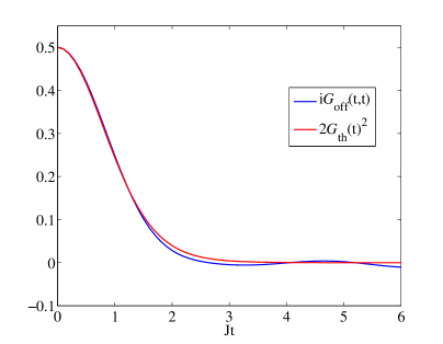
We consider the expectation value of the operator evaluated in Lorentzian time on the state . See figure 3. We see that it decays to zero as we expect for a thermalizing system. But it has small oscillations as we expect in a unitary theory. In a unitary theory this correlator cannot decay to zero for all initial states because a suitable linear combination of initial states should be able to give us a state with eigenvalue at any time. For a detailed analysis of the long time behavior in SYK see [16]. We have also compared the answer to the twice the square of the thermal correlator, as predicted by (3.14). They match fairly closely despite the relatively low value of .
5.3 Entanglement entropy of subsystems
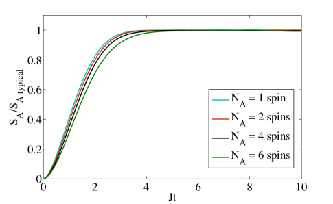
Here we consider the boundary state and we evolve it in Lorentzian time. We can organize the Hilbert space as a tensor product of qubits, viewing the first qubit as the one whose is given by , and similarly with the other qubits. More precisely, we represent the in terms of qubits by a Jordan Wigner transformation555Explicitly: . , and then we look at the tensor decomposition of the Hilbert space in terms of the Hilbert spaces of each of these qubits. The initial state is simple in terms of these qubits because it obeys a condition . It is a factorized state. However, the evolution by the SYK Hamiltonian gives us general linear combinations of states with definite spins. So if we consider the subfactor of the Hilbert space generated by the first few qubits, the initial state is unentangled with the rest, but it will become entangled under time evolution. In fact, it becomes rapidly entangled as in a typical state of the Hilbert space [17]. By rapidly, we mean a time of order , which is the characteristic interaction time. Interestingly, the time to reach the typical entanglement is independent of the size of the subsystem666We thank D. Stanford for emphasizing this point to us.. This fact was demonstrated analytically at large in [18], by showing that the density matrix for a subset of spins factorizes at large (see also [19, 20, 21]). In figure (4) we see a plot of the ratio of these entanglement entropies to the values we expect for a typical state in the Hilbert space, as computed in [17]. For , this typical entanglement entropy is close to maximal, , where is the number qubits of the subsystem. However, at finite the typical entanglement is slightly less than maximal. It is given by a formula , computed in [17]. We see in figure (4) that the evolution of entanglement is fairly independent of the subsystem size and that it reaches the maximal value at the same time for all subsystem sizes. Similar subsytem entanglement entropies were computed for the ground state in [22].
5.4 Euclidean correlators at finite
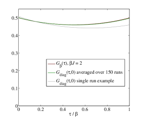
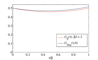
Here we compute the diagonal Euclidean correlators for finite and compare to the thermal answer, also computed at finite . Here we are testing whether (3.13) works at finite . We fix an order one value of so as to have contributions from a large number of states (we are not in the conformal limit). For low values of , such as we have large deviations of order 20 %. However, as becomes large, we get closer results with smaller errors, see figure (5) for examples with . The way the error decreases seems consistent with the scaling777 In the left plot of (5) we are using the normalization in (3.15) where the correlator does not have to be at (at finite ). In the right we used the more natural normalization (3.10) where indeed the correlator is at ..
6 Gravity interpretation
It is interesting to ask whether we can give a gravity interpretation to the above results. At the time of writing, the full bulk dual of the SYK model is unknown. However, we know that general Nearly- gravity or string theory has some features in common with the low energy limit of the SYK model. In particular, in both cases we have an emergent reparametrization symmetry that is both spontaneously and explicitly broken, with an explicit breaking given by the Schwarzian action. A simple Nearly- model is the Jackiw Teitelboim model coupled to matter, see [4, 5, 6, 7] for further discussion.
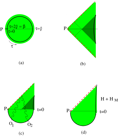
Here we will give a qualitative gravity picture for the solutions we had above. More precisely we will discuss gravity theories with similar features (symmetries) to the ones discussed above. The fact that we continue to have the same diagonal correlators as the thermal state is here interpreted as saying that we continue to have the same geometry as in the Euclidean black hole. In particular, at low energies, we continue to have the same geometry that we had in the thermal case. In Eulidean space we have the hyperbolic disk and we imagine that there is a boundary at some finite but very large circle. See figure 6(a). The new feature is that we have a special point labelled by in figure 6, where we have a kind of defect. We imagine that we have bulk fields and that there is a boundary condition at the marked point that relates the bulk fields in pairs. For example, we can add an interaction of the form for very large which kills all states except the ones with eigenvalue for the operators in (2.3), which are interpreted in the bulk as the product of two fermion fields at the corresponding bulk point. We can also imagine measuring the values of all the fields at the point on the boundary and projecting onto the simultaneous eigenstates of all these measurements888 Complete measurements on an Einstein Rosen bridge were discussed in [23, 24]. . In any case, we are doing a very high energy or UV-like insertion because it is localized at one point P of the boundary circle. At all other points of the boundary circle we have the standard boundary conditions, the same as the ones we have in the thermal state. If we had bulk scalar fields, we can imagine that at , we are putting a source for the bulk scalar fields.
This picture has the advantage of realizing the symmetries of the problem. In fact, we can see this more clearly if we work in the so called poincare coordinates, where we send the point to infinity. The metric can then be written as
| (6.22) |
with Euclidean or Lorentzian signature. The Lorentzian coordinates cover the whole light (and dark) green regions of figure 6(b). On this metric we want to consider a field configuration or a boundary condition at large that is invariant under translations. This is because this was the symmetry preserved by the off diagonal low energy correlator (4.17).
We can continue this configuration to Lorentzian time in various ways. If we just continue in (6.22) we get a zero temperature configuration.
More interestingly, we can continue the metric along a moment of time reflection symmetry and obtain the Rindler coordinates, or finite temperature solution. See figure 6(b). This time reflection symmetry acts as a reflection the leaves fixed the horizontal line passing through point in figure 6. In these coordinates the metric is the same as the one for the thermofield double, but the fields obey different boundary conditions which break some of the isometries of . One important point is that we get a whole region behind the horizon. Notice that only a portion of is visible outside the horizon, the dark green region in figure 6(b).
Furthermore, inserting operators in Euclidean time, we can create more general states on the lorentzian slice. This gives us a precise way to generate states on this slice. Any perturbative state can be produced by a superposition of operator insertions. In particular, we can insert wavefunctions which are localized behind the horizon. Notice that the map between operator insertions on the boundary and the wavefunctions on the bulk is purely kinematical, so we can formally follow the same procedure in the SYK model to define the “bulk wavefunctions”. In the gravity picture we can localize these excitations behind the horizon. When we evolve in Lorentzian signature, such particles will not be visible from the outside. One practical way we can try to see them, is to compute the expectation value of the same field and ask whether it can become significantly large, as it would be the case with a particle that comes out the black hole and hits the boundary. This will not happen for the modes localized behind the horizon if we evolve with the lorentzian SYK hamiltonian as in figure 6(c). This suggests that for each state we have a picture which is similar to a gravity configuration with a smooth horizon. Of course, there is a shock wave some distance behind the horizon999 The distance (or time) to the shock wave becomes very small for an observer who is drops into the black hole at very early times, at lorentzian times . For such observers the starting configuration is one that is complex and it is becoming simpler. As observed in [25] such observers see some kind of firewall. . Though each of the states is special, this set of special states spans the whole Hilbert space. Each of these states is special because they have non-trivial correlators for the operators . These non-trivial correlators decay in time as these states thermalize and become more generic, see figure 3.
6.1 Qualitative connection with other boundary state solutions
In this subsection we consider nearly- gravity configurations containing an end of the world brane. These are configurations that can describe pure states. The end of the world “brane” is a particle in this case. We will see that by tuning its tension to high values we get a configuration that is qualitatively similar to that shown in figure 6(a).
Let us first remind the reader that a simple way to generate a gravity solution dual to a pure state is to take the eternal Schwarzschild solution and perform a quotient that exchanges the left and the right sides, a reflection along a vertical line in the Penrose diagrams, see figure 7(a,a’). Whether we can or cannot do this quotient depends on the full gravity theory in question. In some examples that arise from string theory we can certainly do it and the end of the world branes are the ones familiar in string constructions, see e.g. [26]. We will not discuss the full UV complete gravity theory here, we will simply consider a phenomenological model where we have nearly- gravity and we have an end of the world particle with an arbitrary mass . We generate these configurations by going to a covering space containing a particle of mass and then doing a quotient, where the particle sits as the invariant points. We will see that, as we increase the mass, the effects of gravitational backreaction move this end of the world brane deeper into the left side of the black hole geometry until we get a picture rather similar to the one in figure 6. We will now discuss this in more detail.
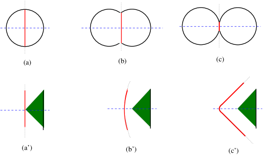
As explained in [10], the gravitational dynamics in nearly- gravity can be expressed in terms of the motion of a boundary particle in a rigid 101010 Do not confuse the boundary of with the actual physical boundary which sits at the location of the boundary particle. The boundary particle is in the interior of but far away from the central region of interest [10].. Therefore, we are looking for a invariant configuration that contains the boundary particle and the particle of mass going between two points on the boundary particle trajectory. The boundary particle emits the massive bulk particle and it absorbes it again later, see figure 7. Computing the classical solution including backreaction amounts to finding particle trajectories of this kind so that the energy momentum is conserved at the vertices. Each of the particle trajectories is specified in terms of their charges, and the energy momentum conservation amounts to the requirement that the total charge is zero [10]. It is convenient to describe in terms of embedding coordinates , . We can also view the charges associated to the particle trajectories as a vector . We can pick the charge for the massive particle as
| (6.23) |
where we have also written the equation for the geodesic trajectory. The boundary particles do not follow geodesics, they move as if they where charged particles of charge and mass in a uniform electric field in 111111 In terms of the parameters of the nearly- gravity theory we have and , where is the ADM mass of the black hole, and we imagine taking [10].. Their trajectories are instead given by [10]
| (6.24) |
The trajectories specified by (6.24) look like circles in Euclidean space where the center is at . The center of these circles is also the position where the future and past horizons intersect in the corresponding Lorentzian black hole. For the problem we are interested in, we expect that these circles will be displaced as in figure 7(b,c). Therefore we make the ansatz
| (6.25) |
where we can view as the displacement of the center of the circle relative to the origin, . Demanding that the sum of the charges is zero we find that
| (6.26) |
But due to (6.24) we find that the size of each circular trajector is given by . In order for to be larger than in (6.26) we need that
| (6.27) |
Which is clear if we think in terms of the balance of forces at the vertex of figure 7(c). The point is that as the two circles become almost tangent to each other, and after the quotient we get a geometry qualitatively similar to that in figure 6(a). This is a large value for , which is comparable to the size of the UV cutoff where the boundary particle sits.
The analytic continuation of these configurations is such that we get a geometry that contains a horizon and an end of the world particle inside the horizon. The trajectory of this particle is following a geodesic in the ambient spacetime. As we move from figure 7(a’) to 7(c’) this is a geodesic that starts closer and closer to the boundary. So as we get to figure 7(c’) it looks like a shock wave.
7 Evolution of the state under a different Hamiltonian
Previously we have claimed that if we start with the state at and evolve it in Lorentzian time, then we get a state that is similar to the gravity configurations in (6)(b,c) which contain a horizon and an inaccessible region behind it.
Here we will show that by evolving with a different Hamiltonian, one that is fine tuned to the particular state that used to prepare the initial state, then we can get a modified evolution for the Schwarzian degree of freedom. Interpreted as a statement in nearly- gravity, this modified evolution is such that it allows us to see behind the horizon. A related modified evolution involving a double trace deformation for pure black holes in is being considered by [8].
This is done as follows. We add to the SYK Hamiltonian (2.1) a new term of the form
| (7.28) |
here is an operator which looks like a “mass term” for the fermions. The factor of in is setting the units so that that is dimensionless121212 The SYK model plus a mass term was discussed in [27, 28].. It is very important for our discussion that we choose the signs in (7.28) to be the same as the ones that describe the state (2.4).
At large we could analyze this problem by solving the real time Schwinger-Dyson equations for the full Hamiltonian (7.28). This was done in [14] for a closely related situation. Here we will further assume that is small enough so that we can first solve the SYK problem and then treat as a small perturbation that will affect only the low energy dynamics of the model. At low energies this dynamics is dominated by the reparametrization mode and we will consider only the effects of this mode.
In other words we simply evaluate the extra term, , on the original state and integrate over reparametrizations
| (7.29) | |||||
| (7.30) |
We now couple the reparametrization mode by transforming in this expression by a reparametrization as in (4.19).
| (7.31) |
where
| (7.32) |
By introducing a Lagrange multiplier, , it is possible to write the total action, which is the Schwarzian (4.21) plus (7.31), as
| (7.33) |
We set to zero while we do the Euclidean evolution to prepare the state and we can turn it on as we start the Lorentzian time evolution at . See figure 6(d). The Euclidean time solution we are interested in is , which sets . 131313 The Euclidean time here is related to the euclidean time in previous sections via .. Since the equation of motion for implies that is constant, we can keep the same constant after we start the Lorentzian evolution.
The Lorentzian evolution is simply the motion of a particle with coordinate on a potential
| (7.34) |
This potential crosses zero at , given by
| (7.35) |
The potential is negative for and positive for . See figure 8.

Furthermore at , , since it is a moment of time reflection symmetry. And the value of at is given by
| (7.36) |
We see that as long as , then the subsequent motion for remains bounded. We will obey this condition as long as is large enough
| (7.37) |
The last inequality comes from the condition that we can trust the reduction of the dynamics to the reparametrization mode. We can obey both conditions in (7.37) as long as .
In terms of the coordinates (6.22) we know that and . Therefore we see that the motion of the boundary along the direction is oscillatory but bounded. In particular, it does not approach (or ). This means that the region that is visible from the boundary is the whole Poincare patch. See figure 6(d).
7.1 Adding particles behind the horizon
As we discussed above, we can add operators during the Euclidean evolution in order to add particles to the original background. We know that we can represent any wavefunction on top of the Hartle-Hawking vacuum by adding a suitable superposition of operators inserted in the lower part of the Euclidean background. Therefore, we can add particles that are either outside or inside the horizon, see figure 6(c). If we evolve with the original SYK Hamiltonian, the same Hamiltonian we used to prepare the state during Euclidean evolution, then the particles behind the horizon are not visible. On the other hand, if we evolve the state with the modified Hamiltonian, then all particles become visible.
7.2 Relation to traversable wormholes
The addition to the Hamiltonian (7.28) is similar to the one that was considered in the problem of traversable wormholes [9, 10]141414In [10] the interaction was turned on only at one time. Here it is turned on for all .. The boundary state is obtained by measuring all the spins on the left half of the thermofield double, giving a result . With this knowledge, an observer on the right half can act with an operator that exploits these results, as in (7.28), and access a larger region of the spacetime. With the interaction considered above, the observer can access the whole region in the Poincare patch instead of just the Rindler patch. Note that the measurement is responsible for creating the shock wave in the bulk.
8 Discussion
In this paper we have looked at a particular set of simple microstates of the SYK model. They are defined by a simple boundary condition for the Majorana fermions. They are also joint eigenvectors of a set of commuting operators . These simple states span a complete basis of the Hilbert space of the model. We have further projected them into a lower energy subspace by performing some amount of Euclidean time evolution.
We found that the “diagonal” correlators are exactly given by the thermal ones. We interpret this as saying that these simple states look completely thermalized from the point of view of the diagonal correlators. This also implies that the expectation values of operators that appear in the OPE at order also have the same expectation values as in the thermal state. This is similar, in spirit, to the fact that these correlatorss for a single value of the couplings is the same, at large , as the average over couplings. Here the correlators for a single state looks similar to the thermal state, which is the average over all states. Some particular off diagonal correlators are not thermalized and know the details about the particular state . As we evolve in Lorentzian time this information is effectively lost as the state thermalizes.
We have discussed some nearly- phenomenological gravity theories that have similar properties. In these gravity theories, the state is a configuration with only one boundary which contains some kind of end of the world particle in the interior. The geometry contains a spacetime region that is causally inaccessible from the outside. In the Lorentzian solution this end of the world particle starts in a region close to where the left boundary would be in in the full wormhole solution and it quickly becomes a high energy shock wave which is at some distance behind the horizon. Observers who fall into the black hole from the right side at positive times experience a smooth horizon.
In the SYK model it is possible to change the Hamiltonian evolution so that the main effects can be captured by the Schwarzian action plus a contribution induced by the extra term in the Hamiltonian. This modification of the evolution for the reparametrization goldstone boson can be interpreted in the bulk as a new trajectory for the boundary. This new trajectory is such that it is possible to see the whole spatial slice of the original state. In particular, we can see the region that previously was behind the horizon. This effect is basically the same as the one that makes wormholes traversable. In fact, there is a precise connection between the two. In the SYK model, we can view the initial state as the one that results from measuring a complete set of commuting operators, on the left side of a thermofield double. Then the modified evolution is essentially the same as the one that was considered in the context of traversable wormholes [9, 10].
It is tempting to conjecture that for more general cases, such as the black hole dual to the D0 brane matrix model [29] (or BFSS matrix model [30]) we have a similar picture. Namely, that a full measurement in the “simple” basis of the UV state at on the left side of the thermofield double state is represented by some operator which is inserted at point in figure (6), so as to give a smooth horizon configuration. It would be nice to check this.
Acknowledgements
We thank A. Almheiri, D. Stanford and Z. Yang for discussions. The thank S. Sachev for a pre-publication copy of [14]. J.M. is supported in part by U.S. Department of Energy grant de-sc0009988. I.K. thanks the Institute for Advanced Studies for hospitality while this work was being finished.
References
- [1] S. Sachdev and J. Ye, “Gapless spin fluid ground state in a random, quantum Heisenberg magnet,” Phys. Rev. Lett. 70 (1993) 3339, arXiv:cond-mat/9212030 [cond-mat].
- [2] A. Kitaev, “A simple model of quantum holography.” http://online.kitp.ucsb.edu/online/entangled15/kitaev/,http://online.kitp.ucsb.edu/online/entangled15/kitaev2/. Talks at KITP, April 7, 2015 and May 27, 2015.
- [3] S. Sachdev, “Strange metals and the AdS/CFT correspondence,” J. Stat. Mech. 1011 (2010) P11022, arXiv:1010.0682 [cond-mat.str-el].
- [4] A. Almheiri and J. Polchinski, “Models of AdS2 backreaction and holography,” JHEP 11 (2015) 014, arXiv:1402.6334 [hep-th].
- [5] K. Jensen, “Chaos and hydrodynamics near AdS2,” arXiv:1605.06098 [hep-th].
- [6] J. Maldacena, D. Stanford, and Z. Yang, “Conformal symmetry and its breaking in two dimensional Nearly Anti-de-Sitter space,” PTEP 2016 no. 12, (2016) 12C104, arXiv:1606.01857 [hep-th].
- [7] J. Engelsöy, T. G. Mertens, and H. Verlinde, “An investigation of AdS2 backreaction and holography,” JHEP 07 (2016) 139, arXiv:1606.03438 [hep-th].
- [8] A. Almheiri, A. Mousatov, and M. Shyani. In progress.
- [9] P. Gao, D. L. Jafferis, and A. Wall, “Traversable Wormholes via a Double Trace Deformation,” arXiv:1608.05687 [hep-th].
- [10] J. Maldacena, D. Stanford, and Z. Yang, “Diving into traversable wormholes,” Fortsch. Phys. 65 no. 5, (2017) 1700034, arXiv:1704.05333 [hep-th].
- [11] J. Maldacena and D. Stanford, “Comments on the Sachdev-Ye-Kitaev model,” arXiv:1604.07818 [hep-th].
- [12] P. Calabrese and J. L. Cardy, “Evolution of entanglement entropy in one-dimensional systems,” J. Stat. Mech. 0504 (2005) P04010, arXiv:cond-mat/0503393 [cond-mat].
- [13] J. Cardy, “Bulk Renormalization Group Flows and Boundary States in Conformal Field Theories,” arXiv:1706.01568 [hep-th].
- [14] A. Eberlein, V. Kasper, S. Sachdev, and J. Steinberg, “Quantum quench of the Sachdev-Ye-Kitaev Model,” arXiv:1706.07803 [cond-mat.str-el].
- [15] D. Stanford. Private communication.
- [16] J. S. Cotler, G. Gur-Ari, M. Hanada, J. Polchinski, P. Saad, S. H. Shenker, D. Stanford, A. Streicher, and M. Tezuka, “Black Holes and Random Matrices,” JHEP 05 (2017) 118, arXiv:1611.04650 [hep-th].
- [17] D. N. Page, “Average entropy of a subsystem,” Phys. Rev. Lett. 71 (1993) 1291–1294, arXiv:gr-qc/9305007 [gr-qc].
- [18] J. M. Magan, “De Finetti theorems and entanglement in large-N theories and gravity,” arXiv:1705.03048 [hep-th].
- [19] J. M. Magan, “Random free fermions: An analytical example of eigenstate thermalization,” Phys. Rev. Lett. 116 no. 3, (2016) 030401, arXiv:1508.05339 [quant-ph].
- [20] J. M. Magan, “Decoherence and Microscopic Diffusion at SYK,” arXiv:1612.06765 [hep-th].
- [21] J. M. Magan, “Black holes as random particles: entanglement dynamics in infinite range and matrix models,” JHEP 08 (2016) 081, arXiv:1601.04663 [hep-th].
- [22] W. Fu and S. Sachdev, “Numerical study of fermion and boson models with infinite-range random interactions,” Phys. Rev. B94 no. 3, (2016) 035135, arXiv:1603.05246 [cond-mat.str-el].
- [23] L. Susskind, “ER=EPR, GHZ, and the consistency of quantum measurements,” Fortsch. Phys. 64 (2016) 72–83, arXiv:1412.8483 [hep-th].
- [24] L. Susskind, “Copenhagen vs Everett, Teleportation, and ER=EPR,” Fortsch. Phys. 64 no. 6-7, (2016) 551–564, arXiv:1604.02589 [hep-th].
- [25] L. Susskind, “The Typical-State Paradox: Diagnosing Horizons with Complexity,” Fortsch. Phys. 64 (2016) 84–91, arXiv:1507.02287 [hep-th].
- [26] J. M. Maldacena, “Eternal black holes in anti-de Sitter,” JHEP 04 (2003) 021, arXiv:hep-th/0106112 [hep-th].
- [27] F. Ferrari. Talk at the conference “Black Holes, Quantum Information, Entanglement and All That”.
- [28] A. M. García-García, A. Romero-Bermúdez, and M. Tezuka, “Stability of chaos in a generalised Sachdev-Ye-Kitaev model,” arXiv:1707.02197 [hep-th].
- [29] N. Itzhaki, J. M. Maldacena, J. Sonnenschein, and S. Yankielowicz, “Supergravity and the large N limit of theories with sixteen supercharges,” Phys. Rev. D58 (1998) 046004, arXiv:hep-th/9802042 [hep-th].
- [30] T. Banks, W. Fischler, S. H. Shenker, and L. Susskind, “M theory as a matrix model: A Conjecture,” Phys. Rev. D55 (1997) 5112–5128, arXiv:hep-th/9610043 [hep-th].