Measurement of the $\pi K$ atom lifetime and the $\pi K$ scattering length

Abstract

After having announced the statistically significant observation (5.6 $\sigma$) of the new exotic $\pi K$ atom, the DIRAC experiment at the CERN proton synchrotron presents the measurement of the corresponding atom lifetime, based on the full $\pi K$ data sample: $\tau=(5.5^{+5.0}_{-2.8})\cdot 10^{-15}s$. By means of a precise relation ($<1\%$) between atom lifetime and scattering length, the following value for the S-wave isospin-odd $\pi K$ scattering length $a_{0}^{-}~{}=~{}\frac{1}{3}(a_{1/2}-a_{3/2})$ has been derived: $\left|a_{0}^{-}\right|=(0.072^{+0.031}_{-0.020})M_{\pi}^{-1}$.

I Introduction

In 2007, the DIRAC collaboration enlarged the scope of the dimesonic atom investigation by starting to search for the strange pion-kaon ($\pi K$) atom. In addition to the ongoing study of $\pi\pi$ atoms, the DIRAC experiment at the CERN proton synchrotron (CERN PS) also collected data containing a kaon beside a pion in the final state. Using all the data since 2007 and optimizing data handling and analysis, the observation of the $\pi K$ atom could be achieved for the first time with a significance of more than 5 standard deviations ADEV16 . On the basis of the same data sample, this paper presents the resulting $\pi K$ atom lifetime and the corresponding $\pi K$ scattering length.

Using non-perturbative lattice QCD (LQCD), chiral perturbation theory (ChPT) and dispersive analysis, the S-wave $\pi\pi$ and $\pi K$ scattering lengths were calculated. S-wave $\pi\pi$ scattering lengths as described in QCD exploiting chiral $SU(2)_{L}\times SU(2)_{R}$ symmetry breaking were confirmed experimentally at a level of about 4% BATE09 ; BATE10 ; ADEV11 . These measurements - independently of their accuracy - cannot test QCD predictions in the strange sector based on chiral $SU(3)_{L}\times SU(3)_{R}$ symmetry breaking. However, this check can be done by investigating $\pi K$ scattering lengths, where the s quark is involved.

The lifetime of the hydrogen-like $\pi K$ atom $A_{K\pi}$ or $A_{\pi K}$, consisting of $\pi^{-}K^{+}$ or $\pi^{+}K^{-}$ mesons, is given by the S-wave $\pi K$ scattering length difference $|a_{1/2}-a_{3/2}|$, where $a_{I}$ is the scattering length for isospin $I$ BILE69 . This atom is an electromagnetically bound state of $\pi^{\mp}$ and $K^{\pm}$ mesons with a Bohr radius of $a_{B}=249$ fm and a ground state Coulomb binding energy of $E_{B}=2.9$ keV. It decays predominantly by strong interaction into the neutral meson pair $\pi^{0}K^{0}$ or $\pi^{0}\overline{K}^{0}$ (Fig. 1).

Figure 1: The dominant decay channel of the $\pi K$ atom. The wavy lines indicate Coulomb photons.

The atom decay width $\Gamma_{1S}$ in the ground state (1S) is determined by the relation BILE69 ; SCHW04 :

$$\Gamma_{1S} =\frac{1}{\tau_{1S}}\simeq\Gamma(A_{K\pi}\to\pi^{0}K^{0}\;\;\text{or}\;\;A_{\pi K}\to\pi^{0}\overline{K}^{0})$$

$$=8\;\alpha^{3}\;\mu^{2}\;p^{*}\;(a_{0}^{-})^{2}\;(1+\delta_{K}),$$ (1)

where the S-wave isospin-odd $\pi K$ scattering length $a_{0}^{-}=\frac{1}{3}(a_{1/2}-a_{3/2})$ is defined in pure QCD for the quark masses $m_{u}=m_{d}$. Further, $\alpha$ is the fine structure constant, $\mu=109$ MeV/$c$ the reduced mass of the $\pi^{\mp}K^{\pm}$ system, $p^{*}=11.8$ MeV/$c$ the outgoing 3-momentum of $\pi^{0}$ or $K^{0}$ ($\overline{K}^{0}$) in the $\pi K$ atom system, and $\delta_{K}$ accounts for corrections, due to isospin breaking, at order $\alpha$ and quark mass difference $m_{u}-m_{d}$ SCHW04 .

A dispersion analysis of $\pi K$ scattering, using Roy-Steiner equations and experimental data in the GeV range, yields $M_{\pi}(a_{1/2}-a_{3/2})=0.269\pm 0.015$ BUET04 , with $M_{\pi}$ as charged pion mass. Inserting $a^{-}_{0}=(0.090\pm 0.005)~{}M_{\pi}^{-1}$ and $\delta_{K}=0.040\pm 0.022$ SCHW04 in (I), one predicts for the $\pi K$ atom lifetime in the ground state

$$\tau=(3.5\pm 0.4)\cdot 10^{-15}~{}\text{s}.$$ (2)

In the framework of $SU(3)$ ChPT WEIN66 ; Gasser85 , $a_{1/2}$ and $a_{3/2}$ were calculated in leading order ($LO$) WEIN66 , 1-loop ($1l$) BERN91 (see also KUBI02 ) and 2-loop order ($2l$) BIJN04 . This chiral expansion can be summarized as follows:

$$M_{\pi}a^{-}_{0} =M_{\pi}a^{-}_{0}(LO)(1+\delta_{1l}+\delta_{2l})$$

$$=M_{\pi}\frac{\mu}{8\pi F_{\pi}^{2}}(1+0.11+0.14)=0.089$$ (3)

with the physical pion decay constant $F_{\pi}$, the 1-loop $\delta_{1l}$ and the 2-loop contribution $\delta_{2l}$. Because of the relatively large s quark mass, compared to u and d quark, chiral symmetry is much more broken, and ChPT is not very reliable at the $\pi K$ threshold. The hope is to get new insights by LQCD. Previously, $\pi K$ scattering lengths were investigated on the lattice with unphysical meson masses and then chirally extrapolated to the physical point. Nowadays, scattering lengths can be calculated directly at the physical point as presented in JANO14 : $M_{\pi}a^{-}_{0}=0.0745\pm 0.0020$. Taking into account statistical and systematic errors, the different lattice calculations JANO14 ; BEAN06 ; Fu12 ; Sasaki14 provide consistent results for $a^{-}_{0}$. Hence, a scattering length measurement could sensitively check QCD (LQCD) predictions.

The production of dimesonic atoms (mesonium) in inclusive high-energy interactions was described in 1985 NEME85 . To observe and study such atoms, the following sequence of physical steps was considered: production rate of atoms and their quantum numbers, atom breakup by interacting electromagnetically with target atoms, lifetime measurement and background estimation. An approach to measure the lifetime, describing the atom as a multilevel system propagating and interacting in the target, was derived in afan96 . It provides a one-to-one relation between the atom lifetime and its breakup probability in the target. By this means, $\pi^{+}\pi^{-}$ AFAN93 ; AFAN94 ; ADEV04 ; ADEV05 ; ADEV11 ; ADEV15 and $\pi K$ atoms ADEV09 ; ADEV14 ; ADEV16 were detected and studied in detail by the DIRAC experiment. The $\pi K$ atom production in proton-nucleus collisions was calculated for different proton energies and atom emission angles GORC00 ; GORC16 . The relativistic $\pi K$ atoms, formed by Coulomb final state interaction (FSI), propagate inside a target and part of them break up (Fig. 2). Particle pairs from breakup, called “atomic pairs” (atomic pair in Fig. 2), are characterised by small relative momenta, $Q<3$ MeV/$c$, in the centre-of-mass (c.m.) system of the pair. Here, $Q$ stands for the experimental c.m. relative momentum, smeared by multiple scattering in the target and other materials and by reconstruction uncertainties. Later, the original c.m. relative momentum $q$ will also be used in the context of particle pair production. In the small $Q$ region, the number of atomic pairs above a substantial background of free $\pi K$ pairs can be extracted.

In the first $\pi K$ atom investigation with a platinum (Pt) target ADEV09 , $173\pm 54$ (3.2 $\sigma$) $\pi K$ atomic pairs were identified. This sample allowed to derive a lower limit on the $\pi K$ atom lifetime of $\tau>0.8\cdot 10^{-15}$ s (90% CL). For measuring the lifetime, a nickel (Ni) target was used because of its breakup probability rapidly rising with lifetime around $3.5\cdot 10^{-15}$ s. This experiment yielded $178\pm 49$ (3.6 $\sigma$) $\pi K$ atomic pairs, resulting in a first atom lifetime and a scattering length measurement ADEV14 : $\tau=(2.5^{+3.0}_{-1.8})\cdot 10^{-15}$ s and $M_{\pi}a^{-}_{0}=0.11^{+0.09}_{-0.04}$. Next, the Pt and Ni data were reprocessed ADEV16 with more precise setup geometry, improved detector response description for the simulation and optimized criteria for the $\pi K$ atomic pair identification. The components of $Q_{T}$, the transverse component of $\vec{Q}$, are labelled $Q_{X}$ and $Q_{Y}$ (horizontal and vertical), and $Q_{L}$ is the longitudinal component. Concerning Pt data, informations from detectors upstream of the spectrometer magnet were included, improving significantly the resolution in $Q_{T}$ compared to the previous analyzis ADEV09 . By analyzing the reprocessed Pt and Ni data, $349\pm 62$ (5.6 $\sigma$) $\pi^{-}K^{+}$ and $\pi^{+}K^{-}$ atomic pairs ADEV16 were observed with reliable statistics and the atom lifetime and scattering length measurement could be improved as presented here.

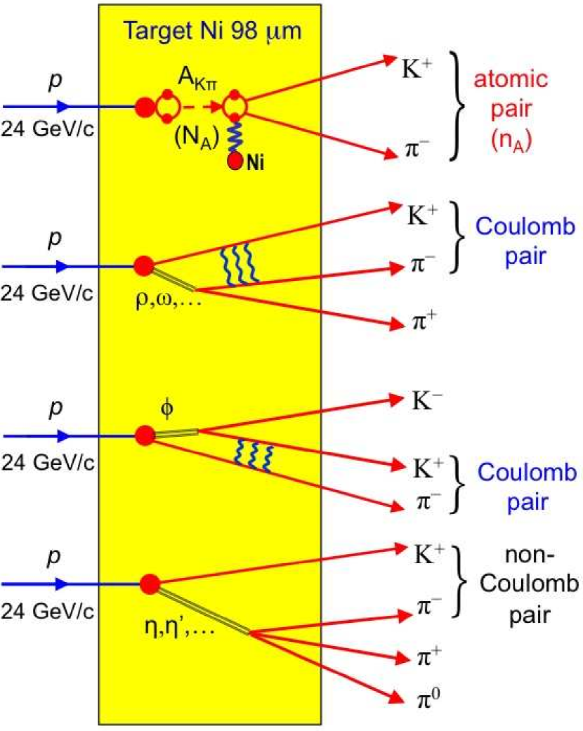
Figure 2: Inclusive $\pi K$ production in the 24 GeV$/c$ p-Ni interaction: p + Ni $\to$ $\pi^{\mp}K^{\pm}$ + X; $A_{K\pi}$ stands for $K^{+}\pi^{-}$ atom.

II Setup and conditions

The aim of the setup is to detect and identify simultaneously $\pi^{-}K^{+}$, $\pi^{+}K^{-}$ and $\pi^{+}\pi^{-}$ pairs with small $Q$. The magnetic 2-arm vacuum spectrometer DIRAC2 (Fig. 3) was optimized for simultaneous detection of these pairs GORC05a ; GORC05b ; PENT15 . The structure of these pairs after the magnet is approximately symmetric for $\pi^{+}\pi^{-}$ and asymmetric for $\pi K$ as sketched in Fig. 3. Originating from a bound system, these pair particles travel with similar velocities, and hence for $\pi K$ the K momentum is by the factor $\frac{M_{K}}{M_{\pi}}=3.5$ larger than the $\pi$ momentum, where $M_{K}$ is the charged kaon mass.

The 24 GeV/$c$ primary proton beam, extracted from the CERN PS, hit in RUN1 a Pt target and in RUN2, RUN3 and RUN4 Ni targets (Table 1). The Ni targets are adapted for measuring the $\pi K$ atom lifetime, whereas the Pt target provides better conditions for the atom observation. With a spill duration of 450 ms, the beam intensity was $(1.5\div 2.1)\cdot 10^{11}$ in RUN1 and $(1.05\div 1.2)\cdot 10^{11}$ protons/spill in RUN2 to RUN4, and the corresponding flux in the secondary channel $(5\div 6)\cdot 10^{6}$ particles/spill.

Table 1: Data and targets

Run Number	1	2	3	4
Year	2007	2008	2009	2010
Run duration	3 months	3 months	5.3 months	5.8 months
Target material	Pt	Ni	Ni	Ni
Target purity (%)	99.95	99.98	99.98	99.98
Target thickness (µm)	$25.7\pm 1$	$98\pm 1$	$108\pm 1$	$108\pm 1$
Radiation thickness ($X_{0}$)	$8.4\cdot 10^{-3}$	$6.7\cdot 10^{-3}$	$7.4\cdot 10^{-3}$	$7.4\cdot 10^{-3}$
Nuclear efficiency	$2.8\cdot 10^{-4}$	$6.4\cdot 10^{-4}$	$7.1\cdot 10^{-4}$	$7.1\cdot 10^{-4}$

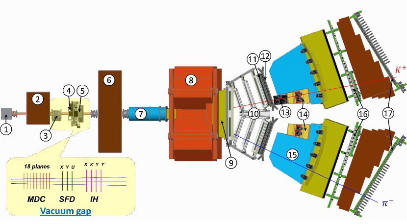
Figure 3: General view of the DIRAC setup (1 – target station; 2 – first shielding; 3 – micro drift chambers (MDC); 4 – scintillating fiber detector (SFD); 5 – ionization hodoscope (IH); 6 – second shielding; 7 – vacuum tube; 8 – spectrometer magnet; 9 – vacuum chamber; 10 – drift chambers (DC); 11 – vertical hodoscope (VH); 12 – horizontal hodoscope (HH); 13 – aerogel Cherenkov (ChA); 14 – heavy gas Cherenkov (ChF); 15 – nitrogen Cherenkov (ChN); 16 – preshower (PSh); 17 – muon detector (Mu).

After the target station, primary protons pass under the setup to the beam dump, whereas secondary particles are confined by the rectangular beam collimator of the second steel shielding wall. The axis of the secondary channel is inclined relative to the proton beam by $5.7^{\circ}$ upward, and the angular divergence in the vertical and horizontal plane is $\pm 1^{\circ}$ (solid angle $\Omega=1.2\cdot 10^{-3}$ sr). Secondary particles propagate mainly in vacuum up to the Al foil $(7.6\cdot 10^{-3}X_{0})$ at the exit of the vacuum chamber, which is installed between the poles of the dipole magnet ($B_{max}$ = 1.65 T and $BL$ = 2.2 Tm).

In the vacuum channel gap, 18 planes of the Micro Drift Chambers (MDC) and ($X$, $Y$, $U$) planes of the Scintillation Fiber Detector (SFD) were installed in order to measure both the particle coordinates ($\sigma_{SFDx}=\sigma_{SFDy}=60$ µm, $\sigma_{SFDu}=120$ µm) and the particle time ($\sigma_{tSFDx}=380$ µm, $\sigma_{tSFDy}=\sigma_{tSFDu}=520~{}\text{ps}$). In RUN1 only the $Y$ and $U$ SFD planes were used. Four planes of the scintillation ionization hodoscope (IH) serve to identify unresolved double tracks (signal only from one SFD column). In RUN1 IH was not in use. The total matter radiation thickness between target and vacuum chamber amounts to $7.7\cdot 10^{-2}X_{0}$.

Each spectrometer arm is equipped with the following subdetectors DIRAC2 : drift chambers (DC) to measure particle coordinates with $\approx$85 µm precision; vertical hodoscope (VH) to measure particle times with 110 ps accuracy to identify particle types via time-of-flight (TOF) measurement; horizontal hodoscope (HH) to select particles with a vertical distance of less than 75 mm ($Q_{Y}$ less than 15 MeV/$c$) in the two arms; aerogel Cherenkov counter (ChA) to distinguish kaons from protons; heavy gas ($\text{C}_{4}\text{F}_{10}$) Cherenkov counter (ChF) to distinguish pions from kaons; nitrogen Cherenkov (ChN) and preshower (PSh) counter to identify $\text{e}^{+}\text{e}^{-}$ pairs; iron absorber; two-layer muon scintillating counter (Mu) to identify muons. In the “negative” arm, no aerogel counter was installed, because the number of antiprotons compared to $K^{-}$ is small.

Pairs of oppositely charged time-correlated particles (prompt pairs) and accidentals in the time interval $\pm 20~{}\text{ns}$ are selected by requiring a 2-arm coincidence (ChN in anticoincidence) with the coplanarity restriction (HH) in the first-level trigger. The second-level trigger selects events with at least one track in each arm by exploiting the DC-wire information (track finder). Using the track information, the online trigger selects $\pi\pi$ and $\pi K$ pairs with relative momenta $|Q_{X}|<12~{}\text{MeV}/c$ and $|Q_{L}|<30~{}\text{MeV}/c$. The trigger efficiency is $\approx$ 98% for pairs with $|Q_{X}|<6~{}\text{MeV}/c$, $|Q_{Y}|<4~{}\text{MeV}/c$ and $|Q_{L}|<28~{}\text{MeV}/c$. Particle pairs $\pi^{-}p$ ($\pi^{+}\bar{p}$) from $\Lambda$ ($\bar{\Lambda}$) decay were used for spectrometer calibration and $\text{e}^{+}\text{e}^{-}$ pairs for general detector calibrations.

III Production of bound and free $\pi^{-}K^{+}$ and $\pi^{+}K^{-}$ pairs

Prompt oppositely charged $\pi K$ pairs, emerging from proton-nucleus collisions, are produced either directly or originate from short-lived (e.g. $\Delta$, $\rho$), medium-lived (e.g. $\omega$, $\phi$) or long-lived sources (e.g. $\eta^{\prime}$, $\eta$). These pion-kaon pairs, except those from long-lived sources, undergo Coulomb FSI resulting in modified unbound states (Coulomb pair in Fig. 2) or forming bound systems in $S$-states with a known distribution of the principal quantum number ($A_{K\pi}$ in Fig. 2) NEME85 . Pairs from long-lived sources are nearly unaffected by the Coulomb interaction (non-Coulomb pair in Fig. 2). The accidental pairs arise from different proton-nucleus interactions.

The cross section of $\pi K$ atom production is given in NEME85 by the expression:

$$\frac{d\sigma^{n}_{A}}{d\vec{p}_{A}} =(2\pi)^{3}\frac{E_{A}}{M_{A}}\left.\frac{d^{2}\sigma^{0}_{s}}{d\vec{p}_{K}d\vec{p}_{\pi}}\right|_{\frac{\vec{p}_{K}}{M_{K}}\approx\frac{\vec{p}_{\pi}}{M_{\pi}}}\cdot\left|\psi_{n}(0)\right|^{2}$$

$$=(2\pi)^{3}\frac{E_{A}}{M_{A}}\frac{1}{\pi a_{B}^{3}n^{3}}\left.\frac{d^{2}\sigma^{0}_{s}}{d\vec{p}_{K}d\vec{p}_{\pi}}\right|_{\frac{\vec{p}_{K}}{M_{K}}\approx\frac{\vec{p}_{\pi}}{M_{\pi}}}\>,$$ (4)

where $\vec{p}_{A}$, $E_{A}$ and $M_{A}$ are the momentum, energy and rest mass of the $A_{K\pi}$ atom in the laboratory system, respectively, and $\vec{p}_{K}$ and $\vec{p}_{\pi}$ the momenta of the charged kaon and pion with equal velocities. Therefore, these momenta obey in good approximation the relations $\vec{p}_{K}=\frac{M_{K}}{M_{A}}\vec{p}_{A}$ and $\vec{p}_{\pi}=\frac{M_{\pi}}{M_{A}}\vec{p}_{A}$. The inclusive production cross section of $\pi K$ pairs from short-lived sources without FSI is denoted by $\sigma_{s}^{0}$, and $\psi_{n}(0)$ is the $S$-state atomic Coulomb wave function at the origin with the principal quantum number $n$. According to (III), $\pi K$ atoms are only produced in $S$-states with probabilities $W_{n}~{}=~{}\frac{W_{1}}{n^{3}}$: $W_{1}~{}=~{}83.2\%$, $W_{2}~{}=~{}10.4\%$, $W_{3}~{}=~{}3.1\%$, $\dots$ , $W_{n>3}~{}=~{}3.3\%$. In complete analogy, the production of free oppositely charged $\pi K$ pairs from short- and medium-lived sources, i.e. Coulomb pairs, is described in the pointlike production approximation by

$$\frac{d^{2}\sigma_{C}}{d\vec{p}_{K}d\vec{p}_{\pi}} =\frac{d^{2}\sigma^{0}_{s}}{d\vec{p}_{K}d\vec{p}_{\pi}}\cdot A_{C}(q)\quad\text{with}$$

$$A_{C}(q) =\frac{2\pi m_{\pi}\alpha/q}{1-\exp\left(-2\pi m_{\pi}\alpha/q\right)}\;.$$ (5)

The Coulomb enhancement function $A_{C}(q)$ in dependence on the relative momentum $q$ (see above) is the well-known Gamov-Sommerfeld-Sakharov factor GAMO28 ; SOMM31 ; SAKH91 . The relative yield between atoms and Coulomb pairs AFAN99 is given by the ratio of equations (III) and (III). The total number $N_{A}$ of produced $A_{\pi K}$ is determined by the model-independent relation

$$N_{A}= K(q_{0})N_{C}(q\leq q_{0})\quad\text{with}$$

$$K(q_{0}=3.12~{}\text{MeV}/c)=0.615\>,$$ (6)

where $N_{C}(q\leq q_{0})$ is the number of Coulomb pairs with $q\leq q_{0}$ and $K(q_{0})$ a known function of $q_{0}$.

Up to now, the pair production was assumed to be pointlike. In order to check finite size effects due to the presence of medium-lived resonances ($\omega$, $\phi$), a study about non-pointlike particle pair sources was performed LEDN08 ; note1205 . Due to the large value of the Bohr radius $a_{B}=249$ fm, the pointlike treatment of the Coulomb $\pi K$ FSI is valid for directly produced pairs as well as for pairs from short-lived strongly decaying resonances. This treatment, however, should be adjusted for pions and kaons originating from decays of medium-lived particles with path lengths comparable with $a_{B}$ in the c.m. system. Furthermore, strong FSI should be taken into account: elastic $\pi^{+}K^{-}\rightarrow\pi^{+}K^{-}$ or $\pi^{-}K^{+}\rightarrow\pi^{-}K^{+}$ (driven at $q\rightarrow 0$ by the $S$-wave scattering length 0.137 fm) and inelastic scattering $\pi^{0}\bar{K^{0}}\rightarrow\pi^{+}K^{-}$ or $\pi^{0}K^{0}\rightarrow\pi^{-}K^{+}$ (scattering length 0.147 fm). In Fig. 4, the simulated distribution of the production regions LEDN08 ; note1205 is shown. Corrections to the pointlike Coulomb FSI can be performed by means of two correction factors $1+\delta(q)$ and $1+\delta_{n}$ ($n$ = principal quantum number), to be applied to the calculated pointlike production cross sections of Coulomb $\pi K$ pairs (III) and S-state $\pi K$ atoms (III), correspondingly LEDN08 ; note1205 .

Figure 4: Predicted distribution of the relative distance $r^{*}$ between the production points for $\pi K$ pairs. The individual curves with increasing $r^{*}$ correspond to pairs produced directly plus from short-lived sources and from $\phi$, $\omega$ and $\eta^{\prime}$ mesons. The sum curve is also shown.

IV Propagation of $\pi K$ atoms through the target

To evaluate the $A_{\pi K}$ lifetime from the experimental value of the $A_{\pi K}$ breakup probability $P_{\mathrm{br}}$, it is necessary to know $P_{\mathrm{br}}=f(\tau,l,Z,p_{A})$ as a function of $A_{\pi K}$ lifetime $\tau$, target thickness $l$, material atomic number $Z$ and lab atom momentum $p_{A}$. After fixing $l$ and $Z$ in accordance with the experimental conditions and integrating $f(\tau,l,Z,p_{A})$ with the measured distribution of $p_{A}$, the dependence $P_{\mathrm{br}}=f(\tau)$ is obtained.

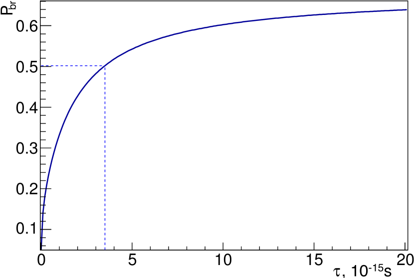
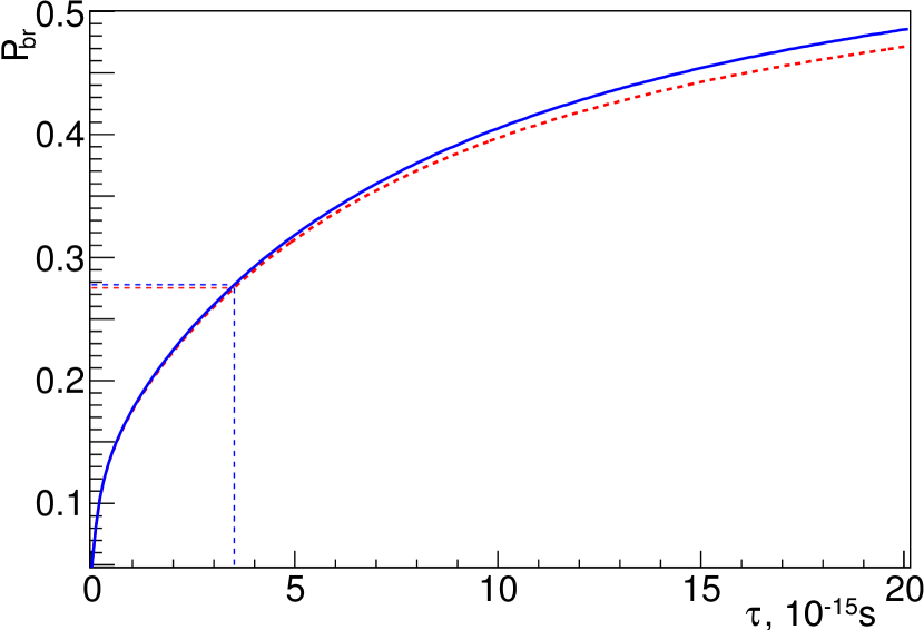
Figure 5: Breakup probability as a function of $\pi K$ atom lifetime $\tau$ (ground state) in the DIRAC experiment. Top: Pt target of thickness 25.7 µm. Bottom: Ni targets of thicknesses 98 µm (red dashed line) and 108 µm (solid blue line). The predicted lifetime $\tau=3.5\cdot 10^{-15}$ s (2) corresponds to the breakup probabilities $P_{\mathrm{br}}$ = 0.50 (Pt) and 0.28 (Ni).

To calculate $f(\tau,l,Z,p_{A})$, one needs to know the total interaction cross sections $\sigma_{\mathrm{tot}}(n,l,m)$ of $A_{\pi K}$ with matter (ordinary) atoms and all transition (excitation/deexcitation) cross sections $\sigma_{if}(n_{i},l_{i},m_{i};n_{f},l_{f},m_{f})$ for a large set of initial $i$ and final $f$ $A_{\pi K}$ states ($n$ principal, $l$ orbital and $m$ magnetic quantum number). In the consideration below, all states with $n\leq 10$ were accounted for. Using these cross sections, the distribution of the atom quantum numbers at production (III) and as free parameter the $A_{\pi K}$ lifetime $\tau$, the evolution of each initial $n$S state from the production point up to the end of the target is described in order to calculate the ionization or breakup probability $P_{\mathrm{br}}$ (Fig. 5).

IV.1 Interaction cross sections of $\pi K$ and $\pi\pi$ atoms with matter atoms

The cross sections of $A_{\pi K}$ interaction with matter atoms were determined from analogous theoretical studies about $\pi^{+}\pi^{-}$ atoms ($A_{2\pi}$) interacting with matter atoms: the $A_{2\pi}$ wave functions are replaced in all formulas by the $A_{\pi K}$ wave functions. The interaction of $A_{2\pi}$ with target atoms includes two parts: 1) interaction with screened nuclei, i.e. coherent scattering, that leaves the target atom in the initial state and 2) interaction with orbital electrons, i.e. incoherent scattering, where the target atom will be excited or ionized. The former is proportional to the square of the nuclear charge ($Z^{2}$), while the latter is proportional to the number of electrons ($Z$). Thus, the latter contribution is insignificant for large $Z$. The cross sections $\sigma_{\mathrm{tot}}$ and $\sigma_{if}$ for the coherent interaction are calculated in first Born approximation (one-photon exchange) by describing the target atoms in the Thomas-Fermi model with Moliere parameterisation afan96 ; KOTS80 ; KOTS83 ; MROW86 ; MROW87 . The $\sigma_{if}$ values taking in to account coherent interaction as well as the incoherent interactions with more precise non-relativistic Hartree-Fock wave functions were calculated in afan96 . For Ni targets, the incoherent contribution to the cross sections is about 4% of the coherent one. The influence of relativistic effects on the $\sigma_{if}$ accuracy was studied basel00 ; basel01 ; basel02 by describing the ordinary atom with the relativistic Dirac-Hartree-Fock-Slater wave functions. Different models for the Ni atom potential lead to an uncertainty in $P_{\mathrm{br}}$ of about 1% DN201406 .

In the $A_{2\pi}$ c.m. system, a target atom creates a scalar and a vector potential. The interaction with the vector potential (magnetic interaction) was discussed in MROW87 ; basel00 ; basel01 . The “magnetic” contribution to the cross sections was calculated in Afan02 . It was shown that “magnetic” contribution to the cross sections for Ni is about 1% of the “electric” one for $A_{2\pi}$ and about 2% for $A_{\pi K}$. All the small cross section corrections discussed here are about twice larger for $A_{\pi K}$ than for $A_{2\pi}$.

Applying the eikonal (Glauber) approach, the next step in accuracy for the mesonium–atom interaction cross sections has been achieved Taras91 ; Voskr98 ; basel01 ; basel02 . This method includes multi-photon exchange processes in comparison with the single-photon exchange in the first Born approximation. The total cross sections for the mesonium interaction with ordinary atoms were calculated. The interaction cross sections for Ni in this approach are less than in the first Born approximation by 0.8% for $n=1$ and at most 1.5% for $n=6$ Afan99jp ; Ivan99 . Therefore, the inclusion of multi-photon exchanges is only relevant in calculations of $\sigma_{if}$ at the 1% level. In the above calculations, the target atoms are considered isolated, i.e. no solid state modification is applied to the wave functions. A dedicated analysis basel01 proves that solid-state effects and target chemistry do not change the $A_{2\pi}$ cross sections. In the mentioned cross section calculations, the $A_{2\pi}$ wave functions are the hydrogen-like non-relativistic Schrödinger equation solutions. The relativistic Klein–Gordon equation for the $A_{2\pi}$ description leads to negligible relativistic corrections to the cross sections basel00 . Furthermore, the seagull diagram contribution can be safely neglected hadatom01 .

IV.2 $\pi K$ and $\pi\pi$ atom breakup probabilities

The description of the $A_{\pi K}$ (multilevel atomic system) propagation in (target) matter is almost the same as in the case for $A_{2\pi}$, first considered in afan96 . $A_{2\pi}$, produced in proton-nucleus collisions, can either annihilate or interact with target atoms. It was shown that stationary atomic states are formed between two successive interactions, at least for $n\leq 6$. Thus, the population of each level can be described in terms of probabilities, disregarding interferences between degenerated states with the same energy. The population of atomic $A_{2\pi}$ states, moving in the target, is described by a set of differential (kinetic) equations, accounting for the $A_{2\pi}$ interaction with target atoms and the $A_{2\pi}$ annihilation. The set of kinetic equations, formally containing an infinite number of equations, is truncated up to states with $n\leq 7$ to get a numerical solution. The breakup probability $P_{\mathrm{br}}$ is calculated by applying the unitary condition:

$$P_{\mathrm{br}}+P_{\mathrm{dsc}}(n\leq 7)+P_{\mathrm{dsc}}(n>7)+P_{\mathrm{ann}}=1,$$

where $P_{\mathrm{dsc}}(n\leq 7)$ and $P_{\mathrm{dsc}}(n>7)$ are the populations of the discrete $A_{2\pi}$ states, leaving the target, with $n\leq 7$ and $n>7$, and $P_{\mathrm{ann}}$ is the $A_{2\pi}$ annihilation probability in the target. Values of $P_{\mathrm{dsc}}(n\leq 7)$ and $P_{\mathrm{ann}}$ are obtained by solving the truncated set of kinetic equations. On the other hand, one gets a value of $P_{\mathrm{dsc}}(n>7)$ by extrapolating the calculated behaviour of $P_{\mathrm{dsc}}(n)$. The value of $P_{\mathrm{dsc}}(n>7)$ is about 0.006, and the extrapolation accuracy is insignificant for the accuracy of $P_{\mathrm{br}}$. The method here only uses total cross sections and transition cross sections between discrete $A_{2\pi}$ states.

Obtaining the ionization (breakup) cross sections for an arbitrary $A_{2\pi}$ bound state basel99 ; basel00 , allows to calculate directly $P_{\mathrm{br}}$ Zhab08 . The difference of 0.5% between two methods for $n=8$ demonstrates the convergence and estimates the $P_{\mathrm{br}}$ precision.

To clarify the influence of the interference between degenerated states with the same energy, the motion of $A_{2\pi}$ in the target was described in the density matrix formalism Voskr03 . The $P_{\mathrm{br}}$ value calculated using this method coincides with the one in the probability based approach with an accuracy of better than $10^{-5}$ Afan04 . The same is true for $A_{\pi K}$.

The function $P_{\mathrm{br}}=f(\tau,l,Z,p_{A})$ has a weak dependence on the target thickness $l$ in the conditions of the DIRAC experiment. The relative $l$ uncertainty of $\pm$1% leads to an insignificant error of $f(\tau,l,Z,p_{A})$ on the level of $\pm$0.1%.

In the present article, $P_{\mathrm{br}}=f(\tau,l,Z,p_{A})$ is calculated by means of the DIPGEN code DIPGEN , using the unitary condition and the set of $A_{\pi K}$ total and transition cross sections calculated in the approach of Ref. afan96 for $n\leq 10$ without taking into account the incoherent interaction, magnetic interaction and multi-photon exchange pik-prop . As described above, all these effects contribute to the cross section only at the level of (1–2)% with different signs. The common error of the approximation used is evaluated in the following way. The $A_{2\pi}$ breakup probabilities $P_{\mathrm{br}}^{\pi\pi}$ are determined in the same way as for $A_{\pi K}$ and also using very precise cross sections basel99 ; basel00 ; basel01 ; basel02 considering all types of interactions. The difference in the $P_{\mathrm{br}}^{\pi\pi}$ values is 0.6% pik-prop . For $A_{\pi K}$, the contributions of unaccounted cross sections are larger than for $A_{2\pi}$ (see above). Hence, the difference in $P_{\mathrm{br}}$ is expected to be larger by a factor of around 2. The accuracy of the $P_{\mathrm{br}}$ calculation procedure for Ni is estimated as 0.8% Zhab08 . Therefore, the upper limit of the total uncertainty of $P_{\mathrm{br}}$ for $A_{\pi K}$ cannot exceed 2%, compared to 1% for $A_{2\pi}$ ADEV11 . This value is significantly smaller than the statistical accuracy.

IV.3 Relative momentum distribution of atomic $\pi K$ pairs

The evaluation of the number of the atomic pairs requires the knowledge of their distribution on the relative momentum at the target exit and after the reconstruction. This distribution depends on the atomic quantum numbers at the atom breakup point and the coordinates of this point. The relative momentum distributions of the atomic pairs for different atom quantum numbers have been calculated hadatom01 and were entered into DIPGEN DIPGEN . This distribution is further broadened by multiple scattering of the mesons in the target. The main influence on the distribution of the transverse relative atomic pair momentum at the target exit is due to multiple scattering in the target, whereas the influence from the atomic states is significantly smaller, but nevertheless taken into account in DIPGEN.

V Data processing

The collected events were analyzed with the DIRAC reconstruction program ARIANE Ariane modified for analyzing $\pi K$ data.

V.1 Tracking

Only events with one or two particle tracks in DC of each arm are processed. The event reconstruction is performed according to the following steps:

• One or two hadron tracks are identified in DC of each arm with hits in VH, HH and PSh slabs and no signal in ChN and Mu.

• Track segments, reconstructed in DC, are extrapolated backward to the beam position in the target, using the transfer function of the dipole magnet and the program ARIANE. This procedure provides approximate particle momenta and the corresponding points of intersection in MDC, SFD and IH.

• Hits are searched for around the expected SFD coordinates in the region $\pm 1$ cm corresponding to (3–5) $\sigma_{\mathrm{pos}}$ defined by the position accuracy taking into account the particle momenta. The number of hits around the two tracks is $\leq 4$ in each SFD plane and $\leq 9$ in all three SFD planes. The case of only one hit in the region $\pm 1$ cm can occur because of detector inefficiency (two crossing particles, but one is not detected) or if two particles cross the same SFD column. The latter type of event may be recovered by selecting double ionization in the corresponding IH slab. For RUN1 data collected with the Pt target, the criteria are different: the number of hits is two in the $Y$- and $U$-plane (signals from SFD $X$-plane and IH, which may resolve crossing of only one SFD column by two particles, were not available in RUN1 data).

The momentum of the positively or negatively charged particle is refined to match the $X$-coordinates of the DC tracks as well as the SFD hits in the $X$- or $U$-plane, depending on the presence of hits. In order to find the best 2-track combination, the two tracks may not use a common SFD hit in the case of more than one hit in the proper region. In the final analysis, the combination with the best $\chi^{2}$ in the other SFD planes is kept.

V.2 Setup tuning using $\Lambda$ and $\bar{\Lambda}$ particles

In order to check the general geometry of the DIRAC experiment, the $\Lambda$ and $\bar{\Lambda}$ particles, decaying into ${\rm p}\pi^{-}$ and $\pi^{+}\bar{\rm p}$ in our setup, were used. Details of this study are reported in DN201601 ; lan ; note0516 . Comparing our reconstructed $\Lambda$ mass values with PDG data pdg allows to check the geometrical setup description. The main factors, that can influence the value of the $\Lambda$ mass, are the position of the aluminium (Al) membrane (defining the location of the spectrometer magnetic field relative to the setup detectors) and the angles between each downstream telescope arm axis and the setup axis (secondary particle beam direction). The position of the Al membrane was fixed to $z_{Al}=1433.85$ mm from the centre of the magnet. The orientation of the downstream arm axes should be corrected on average for the right arm by $-0.032$ mrad and for the left arm by $+0.088$ mrad relative to the geodesic measurements. The values, from year to year used, are reported in DN201601 .

Fig. 6 shows the distribution of the $\Lambda$ mass for the RUN3 data and for the corresponding Monte Carlo (MC) simulation. The distributions are fitted with a Gaussian and a second degree polynomial that describes the background.

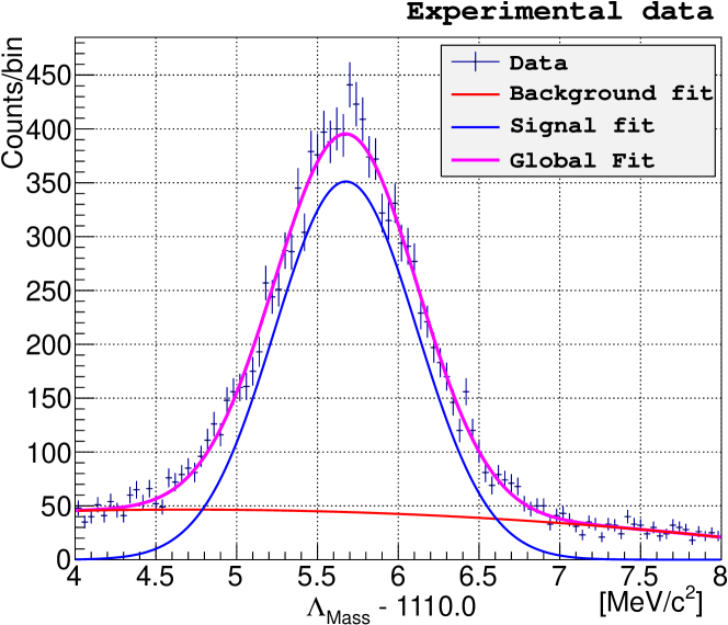
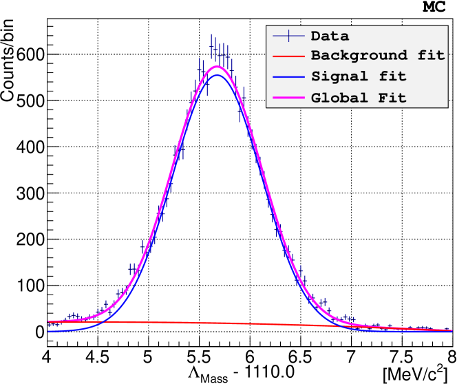
Figure 6: $\Lambda$ mass distribution for RUN3 data (top) and MC simulation (bottom) are fitted with a Gaussian (in blue) for the $\Lambda$ peak and a second degree polynomial (in red) describing the background. $\Lambda^{exp}-1110.0=5.676\pm 5.9\cdot 10^{-3}$ and $\Lambda^{MC}-1110.0=5.675\pm 4.3\cdot 10^{-3}$ in $\rm{MeV}/c^{2}$.

The weighted average value of the experimental $\Lambda$ mass over all runs, $M^{\mathrm{DIRAC}}_{\Lambda}=(1.115680\pm 2.9\cdot 10^{-6})\;\text{GeV}/c^{2}$, agrees very well with the PDG value, $M^{\text{PDG}}_{\Lambda}=(1.115683\pm 6\cdot 10^{-6})\;\text{GeV}/c^{2}$. The weighted average of the experimental ${\bar{\Lambda}}$ mass is $M^{\mathrm{DIRAC}}_{\bar{\Lambda}}=(1.11566\pm 1\cdot 10^{-5})\;\mathrm{GeV}/c^{2}$. This demonstrates that the geometry of the DIRAC setup is well described.

The width of the $\Lambda$ mass distribution allows to test the momentum and angular setup resolution in the simulation. Table  2 shows a good agreement between simulated and experimental $\Lambda$ width. A further test consists in comparing the experimental $\Lambda$ and ${\bar{\Lambda}}$ widths.

Table 2: Standard deviations from Gaussian fit of $\Lambda$ peak in GeV/$c^{2}$ for experimental and MC data and ${\bar{\Lambda}}$ experimental data.

	$\sigma_{\Lambda}$ (data)	$\sigma_{\Lambda}$ (MC)	$\sigma_{\bar{\Lambda}}$ (data)
	$\rm{GeV}/c^{2}$	$\rm{GeV}/c^{2}$	$\rm{GeV}/c^{2}$
RUN1	$4.22\cdot 10^{-4}$	$4.15\cdot 10^{-4}$	$4.3\cdot 10^{-4}$
	${}\pm 4.6\cdot 10^{-6}$	${}\pm 2.9\cdot 10^{-6}$	${}\pm 3\cdot 10^{-5}$
RUN2	$4.33\cdot 10^{-4}$	$4.38\cdot 10^{-4}$	$4.6\cdot 10^{-4}$
	${}\pm 8.2\cdot 10^{-6}$	${}\pm 4.6\cdot 10^{-6}$	${}\pm 2\cdot 10^{-5}$
RUN3	$4.42\cdot 10^{-4}$	$4.42\cdot 10^{-4}$	$4.5\cdot 10^{-4}$
	${}\pm 7.4\cdot 10^{-6}$	${}\pm 4.4\cdot 10^{-6}$	${}\pm 3\cdot 10^{-5}$
RUN4	$4.41\cdot 10^{-4}$	$4.37\cdot 10^{-4}$	$4.3\cdot 10^{-4}$
	${}\pm 7.5\cdot 10^{-6}$	${}\pm 4.5\cdot 10^{-6}$	${}\pm 2\cdot 10^{-5}$

In order to understand, if the differences between data and MC are significant or just due to statistical fluctuations, the MC distributions were generated with a width artificially squeezed and enlarged. In every simulated event, the value of the reconstructed invariant mass of the system pion-proton, $x$, was modified according to $MC_{f}=(x-M_{MC})\cdot f+M_{DATA}$, where $f$ is the parameter shrinking or enlarging the $\Lambda$ distribution by $\pm 20\%$ in steps of 2%. The $\Lambda$ peak positions of the experimental and original MC distributions are denoted by $M_{\mathrm{DATA}}$ and $M_{\mathrm{MC}}$, respectively. Then, the experimental and modified MC distributions were compared CERN-EP-2017-137 . For RUN1 with the Pt target and 2 SFD planes, procedure found the best agreement for $f_{RUN1}=1.019\pm 2.\cdot 10^{-3}$. For the runs with 3 SFD planes and Ni target, the following $f$ values were obtained: $f_{RUN2}=1.00235\pm 4.34\cdot 10^{-3}$, $f_{RUN3}=1.00059\pm 2.75\cdot 10^{-3}$ and $f_{RUN4}=1.00401\pm 3.38~{}\cdot~{}10^{-3}$ with the average value $f_{Ni}=1.00203\pm 0.00191$.

The difference between data and MC widths could be the consequence of imperfectly describing the downstream setup part, to be fixed by a Gaussian smearing of the reconstructed momenta for MC data. On an event–by–event basis, the smearing of the reconstructed proton and pion momentum $p$ has been applied in the form $p^{\mathrm{smeared}}=p(1+C\cdot N(10^{-4}))$, where $N(10^{-4})$ is a normally distributed random number with a mean of 0 and a standard deviation of 0.0001. The values $f_{RUN1}$ and $f_{Ni}$ correspond to $C_{RUN1}=6.7^{+2.2}_{-2.9}$ and $C_{Ni}=2.2319^{+0.7438}_{-1.1758}$, respectively.

The $Q_{L}$ distribution of $\pi^{+}\pi^{-}$ pairs can be used to check the geometrical alignment. Since the $\pi^{+}\pi^{-}$ system is symmetric, the corresponding $Q_{L}$ distribution should be centered at 0. Fig. 7 shows the experimental $Q_{L}$ distribution of pion pairs with transverse momenta $Q_{T}<4~{}\text{MeV}/c$: the distribution is centered at 0 with a precision of 0.2 $\text{MeV}/c$.

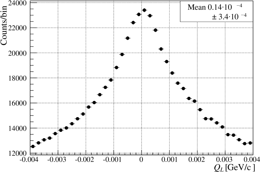
Figure 7: $Q_{L}$ distribution of $\pi^{+}\pi^{-}$ experimental data with cut $Q_{T}<4~{}\text{MeV}/c$ (RUN2 to RUN4).

V.3 Background subtraction

The background of electron-positron pairs is suppressed by ChN at the first level of the trigger system. Because of the large $\text{e}^{+}\text{e}^{-}$ flux and finite ChN efficiency, a certain admixture of $\text{e}^{+}\text{e}^{-}$ pairs with small $Q_{T}$ remains and can induce a bias in the data analysis. To further suppress this background, the preshower scintillation detector PSh is used PENT15 .

At the preparation stage, a set of $\pi^{+}\pi^{-}$ (hadron-hadron) and a set of $\text{e}^{+}\text{e}^{-}$ data were selected by using ChN (low and high amplitude in both arms, respectively). For each pair of PSh slabs ($i$-th slab in the left and $j$-th in the right arm), a procedure selects the amplitude criterion of these slabs accepting 98% of the $\pi^{+}\pi^{-}$ and suppressing $\text{e}^{+}\text{e}^{-}$ pairs. Furthermore, the ratio $R_{ij}$ of $\text{e}^{+}\text{e}^{-}$ events accepted ($N^{\text{accepted}}_{ij}$) and rejected ($N^{\text{rejected}}_{ij}$) by this criterion was calculated for electron trigger data: $R_{ij}=\frac{N^{\text{accepted}}_{ij}}{N^{\text{rejected}}_{ij}}$. In the data analysis, these criteria are applied to the events. Fig. 8a and Fig. 8b present the results for $\text{e}^{+}\text{e}^{-}$ pairs and $\pi^{+}\pi^{-}$ pairs, respectively. The initial distributions are shown as black solid lines and the distributions after applying the PSh amplitude criterion in the left and right arm as red dashed lines. This criterion accepts 97.8% of $\pi^{+}\pi^{-}$ pairs and rejects 87.5% of $\text{e}^{+}\text{e}^{-}$ pairs. To improve the $\text{e}^{+}\text{e}^{-}$ suppression, the remaining electron admixture in the PSh cut data is subtracted from the distribution of accepted events with the event-by-event weight $R_{ij}$. The final distributions are shown as blue dotted lines. The rejection efficiency for the $\text{e}^{+}\text{e}^{-}$ background achieves 99.9%, whereas 2.5% of the $\pi^{+}\pi^{-}$ data are lost.

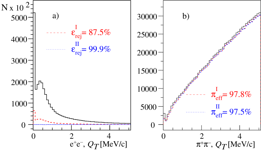
Figure 8: $Q_{T}$ distributions for a) $\text{e}^{+}\text{e}^{-}$ and b) $\pi^{+}\pi^{-}$ pairs without PSh amplitude criterion (black solid line), after amplitude criterion (red dashed line) and after additional subtraction of electron admixture in the accepted events (blue dotted line).

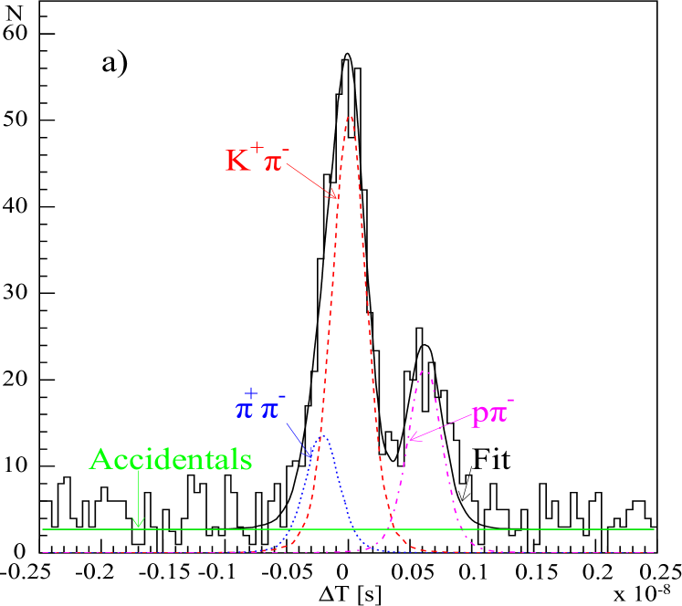
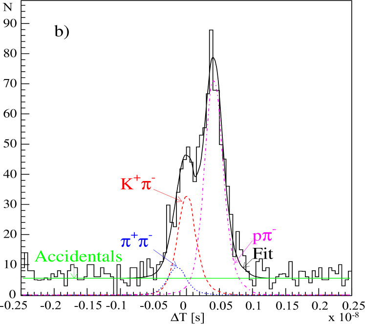
Figure 9: a) Difference of particle generation times for events with positively charged particle momenta $(4.4\div 4.5)~{}\text{GeV}/c$. Experimental data (histogram) are fitted by the event sum (black, solid): $K^{+}\pi^{-}$ (red, dashed), $\pi^{+}\pi^{-}$ (blue, dotted), $\text{p}\pi^{-}$ (magenta, dotted-dashed) and accidentals (green, constant). b) Similar distributions for events with positively charged particle momenta $(5.4\div 5.5)~{}\text{GeV}/c$.

V.4 Event selection criteria

The selected events are classified into three categories: $\pi^{-}K^{+}$, $\pi^{+}K^{-}$ and $\pi^{-}\pi^{+}$. The last category is used for calibration. Pairs of $\pi K$ are cleaned of $\pi^{-}\pi^{+}$ and $\pi^{-}{\rm p}$ background by the Cherenkov counters ChF and ChA (Section II). In the momentum range from 3.8 to 7 $\text{GeV}/c$, pions are detected by ChF with (95–97)% efficiency note1305 , whereas kaons and protons (antiprotons) do not produce any signal. The admixture of $\pi^{-}{\rm p}$ pairs is suppressed by ChA, which records kaons but not protons note0907 . Due to finite detector efficiency, a certain admixture of misidentified pairs still remains in the experimental distributions. For the selected events, the procedure applied plots the distribution of the measured difference $\Delta T$ of particle generation times. These times of production at the target are the times, which are measured by VH and reduced by the time-of-flights from the target to the VH planes for particles with the expected masses ($K^{\pm}$ and $\pi^{\mp}$ mesons) and the measured lab momenta. For $\pi^{-}K^{+}$ ($\pi^{+}K^{-}$) pairs, the difference is centered at 0 and, for misidentified pairs, biased. Fig. 9a presents the event distribution over the difference of the particle production times for $K^{+}$ mesons in the range (4.4–4.5) $\text{GeV}/c$. The distribution is fitted by the simulated distribution of admixed fractions. Similarly to Fig. 9a, Fig. 9b shows the fit for $K^{+}$ in the range (5.4–5.5) $\text{GeV}/c$. The contribution of misidentified pairs was estimated and accordingly subtracted note1306 . Fig. 10a illustrates the $Q_{L}$ distribution of potential $\pi^{-}K^{+}$ pairs requiring a ChF signal and $Q_{T}<4~{}\text{MeV}/c$. The dominant peak on the left side is due to ${\rm p}\pi^{-}$ pairs from $\Lambda$ decay. After requesting a ChA signal, the admixture of ${\rm p}\pi^{-}$ pairs is decreased by a factor of 10 (Fig. 10b). By selecting compatible TOFs between target and VH, background $\text{p}\pi^{-}$ and $\pi^{+}\pi^{-}$ pairs can be substantially suppressed (Fig. 10c). In the final distribution, the well-defined $\pi^{-}K^{+}$ Coulomb peak at $Q_{L}=0$ emerges beside the strongly reduced peak from $\Lambda$ decays at $Q_{L}=-30~{}\text{MeV}/c$.

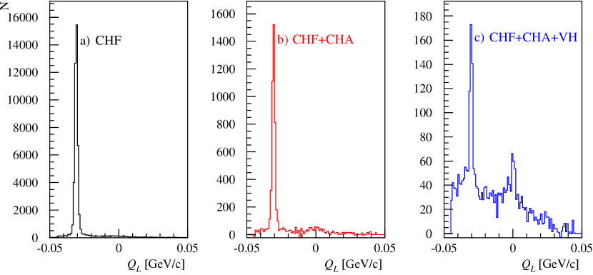
Figure 10: $Q_{L}$ distribution of $\pi^{-}K^{+}$ pairs after applying different criteria (see text).

The $Q_{L}$ distribution of potential $\pi^{+}K^{-}$ pairs shows a similar behaviour CERN-EP-2017-137 . For the final analysis, the DIRAC procedure selects events fulfilling the following criteria:

$$Q_{T}<4\;\text{MeV}/c,\quad|Q_{L}|<20\;\text{MeV}/c\,.$$ (7)

VI Data simulation

VI.1 Multiple scattering simulation

The DIRAC setup as a magnetic vacuum spectrometer has been designed to avoid as much as possible distortions of particle momenta by multiple scattering. Since particles are scattered in the detector planes, it is essential to simulate and reproduce the effect of multiple scattering with a precision better than 1%. A detailed study of multiple scattering has already been performed in the past GORC07 ; msn and been updated msn_new including a new evaluation of thickness and density of the SFD material and additionally cutting on $|Q_{X}|$ and $|Q_{Y}|<4~{}\text{MeV}/c$. This cut has been performed by the trigger for RUN2 and RUN3 allowing a more accurate comparison between data and MC simulation in this region. Prompt $\pi\pi$ pairs were used in order to check the correctness of the multiple scattering description in the simulation. The events were reconstructed, and tracks of positively and negatively charged particles are extrapolated to the target plane: $x_{2}$ ($x_{1}$) and $y_{2}$ ($y_{1}$) are the $\pi^{+}$ ($\pi^{-}$) track coordinates on the target plane. The experimental error in the track measurement and multiple scattering determine the width of $\Delta x=x_{2}-x_{1}$ and $\Delta y=y_{2}-y_{1}$, called vertex resolution. The vertex resolution as a function of the total momentum was studied for particle track pairs with momenta $p_{1}$, $p_{2}$ and velocities $\beta_{1}$, $\beta_{2}$ by using the following parameterisation ($X$ direction):

$$\sigma^{2}_{\Delta x}=c_{1}^{2}+\frac{s_{1}^{2}}{(p_{1}\cdot\beta_{1})^{2}}+c_{2}^{2}+\frac{s_{2}^{2}}{(p_{2}\cdot\beta_{2})^{2}}.$$

Here, $c_{1}$ and $c_{2}$ account for the momentum independent contribution to $\sigma$ (width) of the $x_{1}$ and $x_{2}$ distributions and terms with $s_{1}$ and $s_{2}$ account for the momentum dependent contributions to $\sigma$. Assuming $c_{1}=c_{2}=c$ and $s_{1}=s_{2}=s$, one gets

$$\sigma^{2}_{\Delta x}=2\cdot c^{2}+\left(\frac{1}{(p_{1}\cdot\beta_{1})^{2}}+\frac{1}{(p_{2}\cdot\beta_{2})^{2}}\right)\cdot s^{2}=2\cdot c^{2}+Z\cdot s^{2}.$$

Fig. 11 shows for RUN2 a perfect agreement between data and MC for the $X$ coordinate, the same is valid for the $Y$ coordinate. This procedure, performed for every year of data taking, yields a good agreement with the simulation.

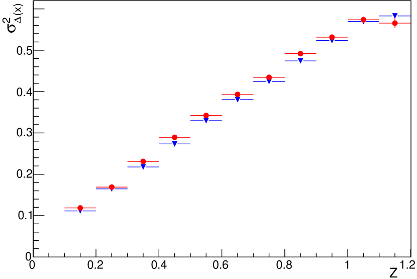
Figure 11: $X$ vertex resolution $\sigma^{2}_{\Delta x}$ in $\rm{cm}^{2}$ as a function of $Z=1/(p_{1}\cdot\beta_{1})^{2}+1/(p_{2}\cdot\beta_{2})^{2}$. Experimental data — blue triangle, MC data — red bullet.

VI.2 SFD response

Track pairs contributing to the signal are characterised by different opening angles, including very small ones. Therefore, it is essential that the SFD detector, which reconstructs upstream tracks, is well described in the simulation.

Figure 12: Left: $\Delta n$ distribution in SFDx for track pairs with small $\Delta n$ in $Y$ ($\Delta n_{Y}<3$). Right: $\Delta n$ distribution in SFDx without any constraint in $Y$. Solid line: experimental data; dotted line: MC data.

From the $\pi^{+}\pi^{-}$ sample outside the signal region $(|Q_{L}|>10~{}\text{MeV}/c)$, track pairs with small opening angles (small distance between SFD hits) were chosen for comparison of experimental and simulated data. To compare experimental and MC data, the events were classified depending on the distance $\Delta n$ between the tracks in SFD column number. As an example, Fig. 12 (left) shows the $\Delta n_{X}$ distribution of very close tracks in $Y$ ($\Delta n_{Y}<3$) and Fig. 12 (right) the $\Delta n_{X}$ distribution without any constraint in $Y$ for data of RUN3. (For more details and data from the other runs, see note1603 .) The remaining difference between experimental and MC data (Fig. 12) is corrected with weights, which depend on the combination of $\Delta n$ in all 3 planes, providing equal $\Delta n$ distributions.

The new MC simulation takes into account: hit efficiency, electronic and photomultiplier noise, cluster size associated with a track and background hits from beam pipe tracks or from particle scattering in the shielding around the detector. These parameters have been evaluated for every run, and the comparison between data and simulation is satisfactory. The SFD multiplicities in the 3 planes are shown in Table 3 for experimental and in Table 4 for MC data.

Table 3: SFD hit multiplicity for experimental data.

RUN	SFDx	SFDy	SFDu
1	–	$3.4\pm 0.7$	$3.0\pm 0.7$
2	$3.6\pm 0.8$	$4.1\pm 1.0$	$3.6\pm 0.8$
3	$3.3\pm 0.8$	$3.7\pm 0.9$	$3.2\pm 0.8$
4	$2.9\pm 0.8$	$3.3\pm 1.0$	$3.0\pm 0.8$

Table 4: SFD hit multiplicity for MC data.

RUN	SFDx	SFDy	SFDu
1	–	$3.5\pm 0.6$	$3.4\pm 0.6$
2	$3.8\pm 0.6$	$4.0\pm 0.6$	$3.7\pm 0.6$
3	$3.3\pm 0.6$	$3.6\pm 0.6$	$3.3\pm 0.6$
4	$3.1\pm 0.8$	$3.4\pm 1.0$	$3.0\pm 0.8$

VI.3 Momentum resolution

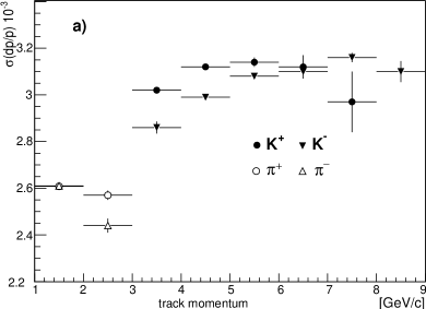
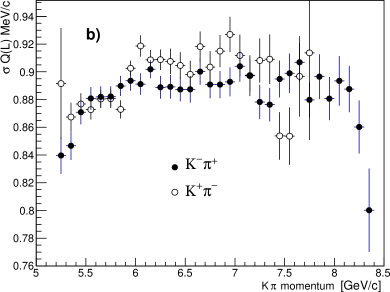
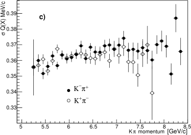
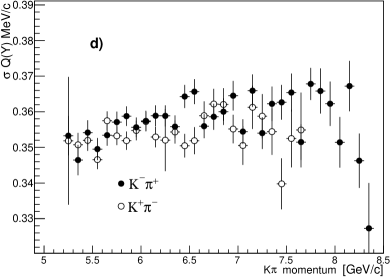
Figure 13: Momentum resolution (a) as a function of the lab particle momentum and resolution of the relative momentum components $Q_{L}$ (b), $Q_{X}$ (c) and $Q_{Y}$ (d) as a function of the total lab momentum of $K^{-}\pi^{+}$ (black) and $K^{+}\pi^{-}$ (white).

Using simulated $\pi K$ events, the momentum resolution is evaluated by means of the expression $\delta_{p}=(p_{\mathrm{gen}}-p_{\mathrm{rec}})/p_{\mathrm{gen}}$, where $p_{\mathrm{gen}}$ and $p_{\mathrm{rec}}$ are the generated and reconstructed momenta, respectively. The additional momentum smearing was taken into account (Section V.2). The resulting $\delta_{p}$ distributions were fitted with a Gaussian, and the standard deviations $\sigma$ of the distributions as a function of the particle momentum $p_{rec}$ are presented in Fig. 13a. In the range from 1 to 8 $\text{GeV}/c$, the DIRAC spectrometer reconstructs lab momenta with a relative precision between $2.4\cdot 10^{-3}$ and $3.2\cdot 10^{-3}$. The resolution of the relative momentum components $Q_{L}$, $Q_{X}$ and $Q_{Y}$ are obtained by MC simulation in the same approach as for the momentum resolution. The results for RUN4 are shown in Fig. 13. For the other runs, the resolutions are similar.

VI.4 Simulation of atomic, Coulomb and non-Coulomb $\pi K$ pair production

Non-Coulomb $\pi K$ pairs, not affected by FSI, show uniform distributions in the c.m. relative momentum projections, whereas Coulomb pairs, exposed to Coulomb FSI, show distributions corresponding to uniform distributions modified by the Gamov-Sommerfeld-Sakharov factor (III). The MC distributions of the lab pair momentum are based on the experimental momentum distributions GORC10 . The $\pi^{+}K^{-}$ were simulated according to $dN/dp=e^{-0.50p}$ and the $\pi^{-}K^{+}$ pairs according to $dN/dp=e^{-0.89p}$, where $p$ is the lab pair momentum in $\text{GeV}/c$. After comparing the experimental with the MC distribution analyzed by the DIRAC program ARIANE, the simulated distributions were modified by applying a weight function in order to fit the experimental data. The lab momentum spectrum of simulated atoms is the same as for Coulomb pairs (III). Numerically solving the transport equations (Section IV), allows to obtain the distributions of the atom breakup points in the target and of the atomic states at the breakup. The latter distribution defines the original c.m. relative momenta $q$ of the produced atomic pairs. The initial spectra of MC atomic, Coulomb and non-Coulomb pairs have been generated by the DIPGEN code DIPGEN . Then, these pairs propagate through the setup according to the detector simulation program GEANT-DIRAC and get analyzed by ARIANE.

The description of the charged particle propagation takes into account (a) multiple scattering in the target, detector planes and setup partitions, (b) the response of all detectors, (c) the additional momentum smearing (Section V.2) and (d) the results of the SFD response analysis (Section VI.2) influencing the $Q_{T}$ resolution.

The propagation of $A_{\pi K}$ through the target is simulated by the MC method. The total amount of atomic pairs is $n_{A}^{MC}(0)$. The full number of simulated Coulomb pairs in the same setup acceptance is $N^{MC}_{C}(0)$, and the amount of Coulomb pairs with relative momenta $q<3.12~{}\text{MeV}/c$ (III) is $N^{MC}_{C}(K)$. These numbers are used for calculating the atom breakup probabilities.

VII Data analysis

VII.1 Number of $\pi^{-}K^{+}$ and $\pi^{+}K^{-}$ atoms and atomic pairs

The analysis of $\pi K$ data is similar to the $\pi^{+}\pi^{-}$ analysis as presented in ADEV11 . For events with $Q_{T}<4~{}\text{MeV}/c$ and $|Q_{L}|<20~{}\text{MeV}/c$ (7), the experimental distributions of $Q$ ($N(Q_{i})$) and of its projections have been fitted for each run and each $\pi K$ charge combination by simulated distributions of atomic ($n^{MC}_{A}(Q_{i})$), Coulomb ($N^{MC}_{C}(Q_{i})$) and non-Coulomb ($N^{MC}_{nC}(Q_{i})$) pairs. The admixture of accidental pairs has been subtracted from the experimental distributions, using the difference of the particle production times (Section V.4). The distributions of simulated events are normalized to 1 by integrating them ($n^{MC}_{A}$, $N^{MC}_{C}$ and $N^{MC}_{nC}$). In the experimental distributions, the numbers of atomic ($n_{A}$), Coulomb ($N_{C}$) and non-Coulomb ($N_{nC}$) pairs are free fit parameters in the minimizing expression:

$$\chi^{2}=\sum_{i}\frac{\left(N(Q_{i})-n_{A}\cdot n^{MC}_{A}(Q_{i})-N_{C}\cdot N^{MC}_{C}(Q_{i})-N_{nC}\cdot N^{MC}_{nC}(Q_{i})\right)^{2}}{\sigma^{2}_{N(Q_{i})}}\,.$$ (8)

The sum of these parameters is equal to the number of analyzed events. The fitting procedure takes into account the statistical errors of the experimental distributions. The statistical errors of the MC distributions are more than one order less than the experimental ones.

Fig. 14a presents the experimental and simulated $Q$ distributions of $\pi K$ pairs for the data obtained from the Pt target and Fig. 15a for Ni data. One observes an excess of events above the sum of Coulomb and non-Coulomb pairs in the low $Q$ region, where atomic pairs are expected: these excess spectra are shown in Figs. 14b and 15b together with the simulated distribution of atomic pairs. The numbers of atomic pairs, found in the Pt and Ni target data, are $n_{A}(\text{Pt})=73\pm 22$ ($\chi^{2}/n=40/36$, $n=$ number of degrees of freedom) and $n_{A}(\text{Ni})=275\pm 57$ ($\chi^{2}/n=40/37$). Comparing the experimental and simulated distributions demonstrates good agreement.

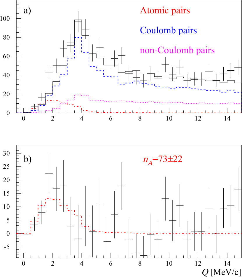
Figure 14: a) Experimental distribution of $\pi^{-}K^{+}$ and $\pi^{+}K^{-}$ pairs (points with error bars) for the platinum (Pt) target fitted by a sum of simulated distributions of “atomic”, “Coulomb” and “non-Coulomb” pairs. The background distribution of free (“Coulomb” and “non-Coulomb”) pairs is shown as black line; b) Difference distribution between the experimental and simulated free pair distributions compared with the simulated distribution of “atomic pairs”.

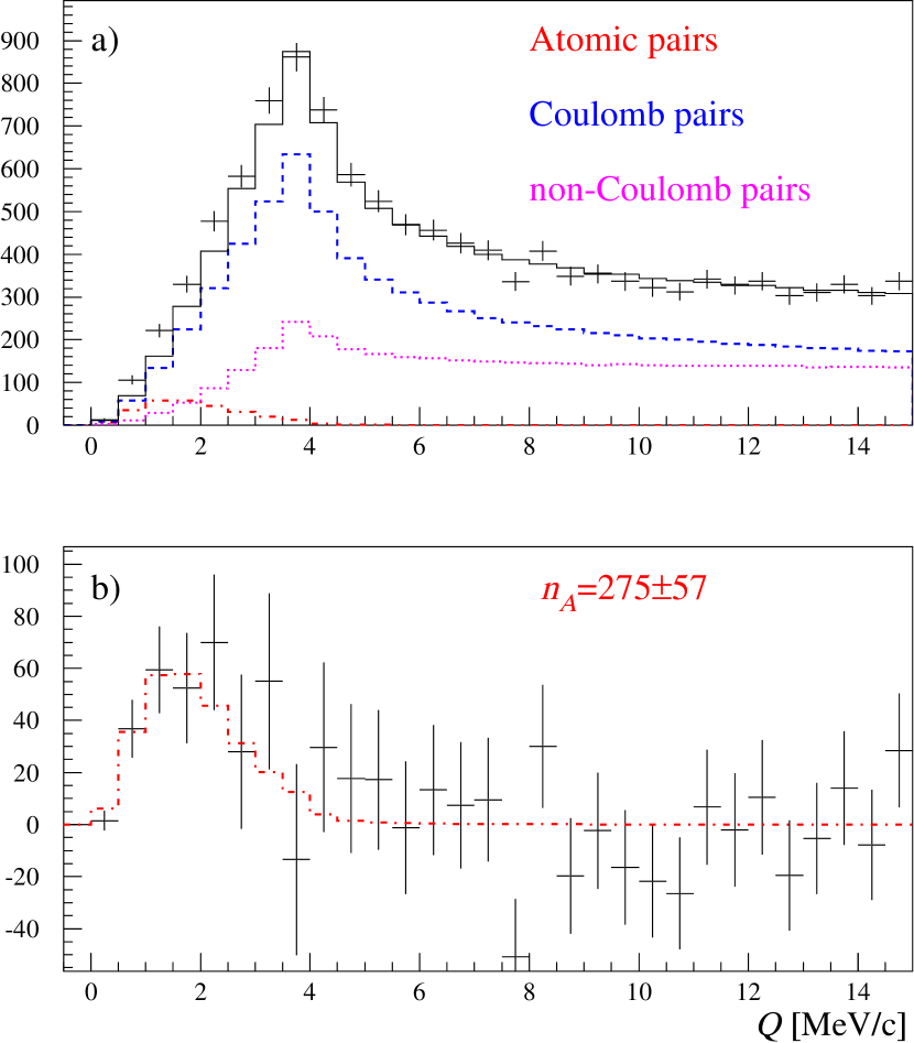
Figure 15: Experimental distribution of $\pi^{-}K^{+}$ and $\pi^{+}K^{-}$ pairs for nickel (Ni) target analogous to Fig. 14.

The same analysis was performed for $\pi^{-}K^{+}$ and $\pi^{+}K^{-}$ pairs, separately. For the Pt target, the numbers of $\pi^{-}K^{+}$ and $\pi^{+}K^{-}$ atomic pairs are $n^{\pi^{-}K^{+}}_{A}(\text{Pt})=57\pm 19$ ($\chi^{2}/n=40/36$) and $n^{\pi^{+}K^{-}}_{A}(\text{Pt})=16\pm 12$ ($\chi^{2}/n=41/36$), and for Ni, the corresponding numbers are $n^{\pi^{-}K^{+}}_{A}(\text{Ni})=186\pm 48$ ($\chi^{2}/n=33/37$) and $n^{\pi^{+}K^{-}}_{A}(\text{Ni})=90\pm 30$ ($\chi^{2}/n=39/37$). The experimental ratios between the two types of atom production are $3.5\pm 2.7$ for Pt and $2.07\pm 0.87$ for Ni. Corrected by the difference of their detection efficiencies, these ratios result in $R^{\pi^{-}K^{+}}_{\pi^{+}K^{-}}(\text{Pt})=3.2\pm 2.5$ and $R^{\pi^{-}K^{+}}_{\pi^{+}K^{-}}(\text{Ni})=2.5\pm 1.0$, compatible with $2.4$ as calculated in the framework of FRITIOF GORC16 . Tables 5 and 6 present these data, comparing them with the results of the $|Q_{L}|$ and the 2-dimensional ($|Q_{L}|$,$Q_{T}$) analyzes. The results of the $Q$ and ($|Q_{L}|$,$Q_{T}$) analyzes are in good agreement, and the 1-dimensional $|Q_{L}|$ analysis does not contradict the values obtained in the other two statistically more precise analyzes.

Table 5: $\pi^{-}K^{+}$ and $\pi^{+}K^{-}$ data for the Pt target: atomic pair numbers $n_{A}$ and ratio $R^{\pi^{-}K^{+}}_{\pi^{+}K^{-}}$ as obtained by analyzing the 1-dimensional $Q$ and $|Q_{L}|$ distributions and the 2-dimensional ($|Q_{L}|$,$Q_{T}$) distribution. Only statistical errors are given.

Analysis	$n_{A}$	$n^{\pi^{-}K^{+}}_{A}$	$n^{\pi^{+}K^{-}}_{A}$	$R^{\pi^{-}K^{+}}_{\pi^{+}K^{-}}$
	($\chi^{2}/n$)	($\chi^{2}/n$)	($\chi^{2}/n$)
$Q$	$73\pm 22$	$57\pm 19$	$16\pm 12$	$3.2\pm 2.5$
	(40/36)	(40/36)	(41/36)
$|Q_{L}|$	$73\pm 31$	$61\pm 27$	$12\pm 16$	$4.7\pm 6.6$
	(37/37)	(40/37)	(28/37)
$|Q_{L}|,Q_{T}$	$71\pm 21$	$65\pm 18$	$6\pm 11$	$10\pm 20$
	(169/154)	(159/151)	(102/135)

Table 6: $\pi^{-}K^{+}$ and $\pi^{+}K^{-}$ data for the Ni targets: atomic pair numbers $n_{A}$ and ratio $R^{\pi^{-}K^{+}}_{\pi^{+}K^{-}}$ analogous to Table 5.

Analysis	$n_{A}$	$n^{\pi^{-}K^{+}}_{A}$	$n^{\pi^{+}K^{-}}_{A}$	$R^{\pi^{-}K^{+}}_{\pi^{+}K^{-}}$
	($\chi^{2}/n$)	($\chi^{2}/n$)	($\chi^{2}/n$)
$Q$	$275\pm 57$	$186\pm 48$	$90\pm 30$	$2.5\pm 1.0$
	(40/37)	(33/37)	(39/37)
$|Q_{L}|$	$157\pm 87$	$103\pm 74$	$55\pm 45$	$2.3\pm 2.5$
	(56/37)	(52/37)	(32/37)
$|Q_{L}|,Q_{T}$	$243\pm 56$	$171\pm 47$	$72\pm 30$	$2.8\pm 1.4$
	(225/157)	(226/157)	(157/157)

The efficiency of atomic pair recording is evaluated from the simulated data as ratio of the MC atomic pair number $n_{A}^{MC}$, passed the corresponding cuts - in each of the above analysis - to the full number of generated atomic pairs: $\varepsilon_{A}=n_{A}^{MC}/n_{A}^{MC}(0)$ (Section VI.4). The full number of atomic pairs, that corresponds to the experimental value $n_{A}$, is given by $n_{A}/\varepsilon_{A}$. In the same way, the efficiency of Coulomb pair recording is $\varepsilon_{C}=N_{C}^{MC}/N_{C}^{MC}(0)$ and the full number of Coulomb pairs $N_{C}/\varepsilon_{C}$. This number allows to calculate the number $N_{A}$ of atoms produced in the target, using the theoretical ratio $K$ (III) and the simulated efficiency $\varepsilon_{K}=N_{C}^{MC}(K)/N_{C}^{MC}(0)$ of the cut $q<3.12~{}\mathrm{MeV}/c$ for Coulomb pairs: $N_{A}=K\cdot\varepsilon_{K}\cdot N_{C}/\varepsilon_{C}$. Thus, the atom breakup probability $P_{\mathrm{br}}$ is expressed via the fit results $n_{A}$, $N_{C}$ and the simulated efficiencies as:

$$P_{\mathrm{br}}=\frac{\frac{n_{A}}{\varepsilon_{A}}}{K\cdot\varepsilon_{K}\frac{N_{C}}{\varepsilon_{C}}}\,.$$ (9)

Table 7 contains the $P_{\mathrm{br}}$ values obtained in the $Q$ and ($|Q_{L}|$,$Q_{T}$) analyzes.

Table 7: Experimental $P_{\mathrm{br}}$ from $Q$ and $(|Q_{L}|,Q_{T})$ analyzes. Only statistical uncertainties are cited.

Data	RUN	Target (µm)	$P^{Q}_{br}$	$P^{|Q_{L}|,Q_{T}}_{br}$
$\pi^{+}K^{-}$	1	Pt (25.7)	$1.2\pm 1.3$	$0.27\pm 0.56$
$\pi^{+}K^{-}$	2	Ni (98)	$0.53\pm 0.39$	$0.42\pm 0.38$
$\pi^{+}K^{-}$	3	Ni (108)	$0.29\pm 0.20$	$0.33\pm 0.24$
$\pi^{+}K^{-}$	4	Ni (108)	$0.33\pm 0.22$	$0.21\pm 0.20$
$\pi^{-}K^{+}$	1	Pt (25.7)	$1.09\pm 0.52$	$1.44\pm 0.59$
$\pi^{-}K^{+}$	2	Ni (98)	$0.32\pm 0.20$	$0.44\pm 0.22$
$\pi^{-}K^{+}$	3	Ni (108)	$0.23\pm 0.16$	$0.16\pm 0.15$
$\pi^{-}K^{+}$	4	Ni (108)	$0.41\pm 0.17$	$0.34\pm 0.16$
$\pi^{+}K^{-}\&K^{+}\pi^{-}$	1	Pt, 25.7	$1.11\pm 0.48$	$0.83\pm 0.41$

VII.2 Systematic errors

Different sources of systematic errors were investigated. Most of them arise from differences in the shapes of experimental and MC distributions for atomic, Coulomb and, to a much lesser extent, for non-Coulomb pairs. The shape differences induce a bias in the values of the fit parameters $n_{A}$ and $N_{C}$, leading to systematic errors of the atomic pair number and finally of the probability $P_{\mathrm{br}}$. In the following, a list of the different sources is presented:

• Resolution over particle momentum of the simulated events is modified by the $\Lambda$ width correction (Section V.2). The parameter $C$, used for additional smearing of measured momenta, is defined with finite accuracy, resulting in a possible difference in resolution of experimental and simulated data over $Q_{L}$.

• Multiple scattering in the targets (Pt and Ni) provides a major part of the $Q_{T}$ smearing. The average multiple scattering angle is known with 1% accuracy. This uncertainty induces a systematic error due to different resolutions over $Q_{T}$ for experimental and simulated data.

• SFD simulation procedure as described in Section VI.2 corrects a residual difference with weights, depending on the distances between particles in the three SFD planes. These weights are estimated by a separate procedure resulting in a systematic error.

• Coulomb pair production cross section increases at low $q$ according to $A_{C}(q)$ (III) assuming a pointlike pair production region. Typical sizes of production regions from medium-lived particle decays [($30\div 40$) fm] are smaller than the Bohr radius (such pairs undergo Coulomb FSI), but not pointlike. In order to check finite size effects due to the presence of medium-lived particles ($\omega$, $\phi$), non-pointlike particle pair sources are investigated, and correlation functions for the different pair sources calculated LEDN08 . The final correlation function, considering the sizes of the pair production regions, has some uncertainty due to limited accurate fractions of the different $\pi K$ sources.

• Uncertainties in the measurement of $\pi^{-}K^{+}$ and $\pi^{+}K^{-}$ pair lab momentum spectra and the relation between these uncertainties and the systematic errors of the atomic pair measurement are described in note1306 . There is a mechanism that increases the influence of the bias between experimental and simulated distributions for $\pi K$ compared to $\pi\pi$. For detected small $Q$ $\pi K$ pairs, kaons have lab momenta $\sim 3.5$ times higher than pions, $(4\div 6)~{}\text{GeV}/c$ compared to $(1.2\div 2)~{}\text{GeV}/c$. The spectrometer acceptance as a function of lab momentum strongly decreases at momenta higher than 3 $\text{GeV}/c$. As a result, kaons with lower momenta are detected more efficiently. In the pair c.m. system, this corresponds to $Q_{L}<0$ for $\pi^{-}K^{+}$ pairs as illustrated in Fig. 10c. For $\pi\pi$, the corresponding distributions consist of the flat horizontal background of non-Coulomb pairs and symmetric peak of Coulomb and atomic pairs. The observed slope for $\pi K$ in $Q_{L}$ distribution is non-linear, that transforms to a non-linear background behavior in $|Q_{L}|$. Thus, the quality of separation between Coulomb and non-Coulomb pairs becomes more sensitive to the accuracy of simulated distributions.

• Uncertainty in the lab momentum spectrum of background pairs results in a similar effect as the uncertainties of $\pi^{-}K^{+}$ and $\pi^{+}K^{-}$ spectra. Both spectra are measured with a time-of-flight based procedure (Section V.3), but as independent parameters. Therefore, the uncertainty of the background pairs is assumed to be an independent source for systematic errors.

• Uncertainty in the $P_{\mathrm{br}}(\tau)$ relation (Section IV.2).

Estimations of systematic errors, induced by different sources, are presented in Table 8 for Pt data and Table 9 for Ni data. The total errors were calculated as the quadratic sum. The procedure of the $\pi K$ atom lifetime estimation described below includes all systematic errors, although their contributions are insignificant compared to the statistical errors.

Table 8: Estimated systematic errors of $P_{\mathrm{br}}$ for Pt in $Q$ and ($|Q_{L}|,Q_{T}$) analyzes.

Source	$Q$	$(|Q_{L}|,Q_{T})$
Uncertainty in $\Lambda$ width correction	0.011	0.073
Uncertainty of multiple scattering in the Pt target	0.0087	0.014
Accuracy of SFD simulation	0.	0.
Correction of the Coulomb correlation function on finite size production region	0.0001	0.0002
Uncertainty in $\pi K$ pair lab. momentum spectrum	0.089	0.25
Uncertainty in the laboratory momentum spectrum of background pairs	0.22	0.21
Uncertainty in the $P_{\mathrm{br}}(\tau)$ relation	0.01	0.01
Total	0.24	0.34

Table 9: Estimated systematic errors of $P_{\mathrm{br}}$ for Ni in $Q$ and ($|Q_{L}|,Q_{T}$) analyzes.

Source	$Q$	$(|Q_{L}|,Q_{T})$
Uncertainty in $\Lambda$ width correction	0.0006	0.0006
Uncertainty of multiple scattering in a Ni target	0.0051	0.0036
Accuracy of SFD simulation	0.0002	0.0003
Correction of the Coulomb correlation function on finite size production region	0.0001	0.0000
Uncertainty in $\pi K$ pair lab. momentum spectrum	0.0052	0.0050
Uncertainty in the laboratory momentum spectrum of background pairs	0.0011	0.0011
Uncertainty in the $P_{\mathrm{br}}(\tau)$ relation	0.0055	0.0055
Total	0.0092	0.0084

VII.3 $\pi K$ atom lifetime and $\pi K$ scattering length measurements

The $\pi K$ atom breakup probabilities $P_{\mathrm{br}}=f(\tau,l,Z,p_{A})$ in the different targets are presented in Section IV.2 and have been calculated for the Ni (98 µm, 108 µm) and the Pt (26 µm) targets. For each target, $P_{\mathrm{br}}$ is evaluated for $\pi^{+}K^{-}$ and $\pi^{-}K^{+}$ atoms, separately, taking into account their lab momentum distributions. For estimating the lifetime of $A_{\pi K}$ in the ground state, the maximum likelihood method daniel08 is applied DN201606 :

$$L(\tau)=\exp\left(-U^{T}G^{-1}U/2\right),$$ (10)

where $U_{i}=\Pi_{i}-P_{\mathrm{br},i}(\tau)$ is a vector of differences between measured $\Pi_{i}$ ($P_{\mathrm{br}}$ in Table 7) and corresponding theoretical breakup probability $P_{\mathrm{br},i}(\tau)$ for a data sample $i$. The error matrix of $U$, named $G$, includes statistical ($\sigma_{i}$) as well as systematic uncertainties. Only the term corresponding to the uncertainty in the $P_{\mathrm{br}}(\tau)$ relation is considered as correlated between the Ni and Pt data, which is a conservative approach and overestimates this error. The other systematic uncertainties do not exhibit a correlation between the data samples from the Ni and Pt targets. On the other hand, systematic uncertainties of the Ni data samples are correlated.

The likelihood functions of the $(|Q_{L}|,Q_{T})$ and $Q$ analyzes are shown in Fig. 16, and Table 10 summarizes the results of both analysis types and for different cuts in the $Q$ space. One realizes that the usage of the Pt data in the analysis does not significantly modify the final result. As the magnitude of the systematic error for Pt is only about 2 times smaller than the statistical uncertainty, the inclusion of systematic errors changes the relative weights of the Pt and Ni data samples, thus shifting the best estimate for $\tau_{\text{tot}}$ with respect to $\tau_{\text{stat}}$. The introduction of the criteria $|Q_{x}|,|Q_{y}|<4\>\text{MeV}/c$ increases the background level by 22%, relative to the criterion $Q_{T}<4\>\text{MeV}/c$. The results in Table 10 show that the lifetime values obtained with the $Q$ analysis are practically equal for both criteria. Therefore, the final result is presented for the $Q$ analysis evaluated with the criterion $Q_{T}<4\>\text{MeV}/c$, using the statistics of the Ni and Pt data samples:

$$\tau_{\text{tot}}=\left.(5.5^{+5.0}_{-2.8}\right|_{\text{tot}})\cdot 10^{-15}~{}\text{s}.$$ (11)

The measured $\pi K$ atom lifetime corresponds, according to the relation (I) (Fig. 17), to the following value of the $\pi K$ scattering length $a_{0}^{-}$:

$$\left|a_{0}^{-}\right|M_{\pi}=\left.0.072^{+0.031}_{-0.020}\right|_{\text{tot}}.$$ (12)

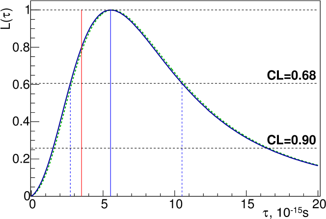
Figure 16: Likelihood functions $L(\tau)$ for $Q$ analyzes with $Q_{T}<4\>\text{MeV}/c$. The likelihood functions on the basis of both statistical and systematic errors (dashed green line) and on the basis of only statistical error (solid blue line) are presented. The vertical blue lines indicate the best estimate for $\tau_{\text{tot}}$ and the corresponding confidence interval. The vertical red line is the theoretical prediction (2).

Table 10: $\pi K$ atom lifetime measurements: $\tau_{\text{stat}}$ (only statistical error) and $\tau_{\text{tot}}$ (total error) in $10^{-15}$ s.

Analysis	Cuts	Target	$\tau_{\text{stat}}$	$\tau_{\text{tot}}$
$(|Q_{L}|,Q_{T})$	$Q_{T}<4\>\text{MeV}/c$	Pt&Ni	$3.96^{+3.49}_{-2.12}$	$3.79^{+3.48}_{-2.12}$
$(|Q_{L}|,Q_{T})$	$Q_{T}<4\>\text{MeV}/c$	Ni	$3.52^{+3.40}_{-2.10}$	$3.52^{+3.42}_{-2.11}$
$(|Q_{L}|,Q_{T})$	$|Q_{x}|,|Q_{y}|<4\text{MeV}/c$	Pt&Ni	$3.16^{+2.67}_{-1.73}$	$2.89^{+2.63}_{-1.70}$
$(|Q_{L}|,Q_{T})$	$|Q_{x}|,|Q_{y}|<4\text{MeV}/c$	Ni	$2.66^{+2.56}_{-1.66}$	$2.66^{+2.58}_{-1.66}$
$Q$	$Q_{T}<4\>\text{MeV}/c$	Pt&Ni	$5.64^{+4.99}_{-2.82}$	$5.53^{+4.98}_{-2.81}$
$Q$	$Q_{T}<4\>\text{MeV}/c$	Ni	$5.07^{+4.73}_{-2.74}$	$5.07^{+4.77}_{-2.75}$
$Q$	$|Q_{x}|,|Q_{y}|<4\text{MeV}/c$	Pt&Ni	$5.62^{+4.65}_{-2.71}$	$5.60^{+4.68}_{-2.72}$
$Q$	$|Q_{x}|,|Q_{y}|<4\text{MeV}/c$	Ni	$4.98^{+4.37}_{-2.60}$	$4.98^{+4.41}_{-2.62}$

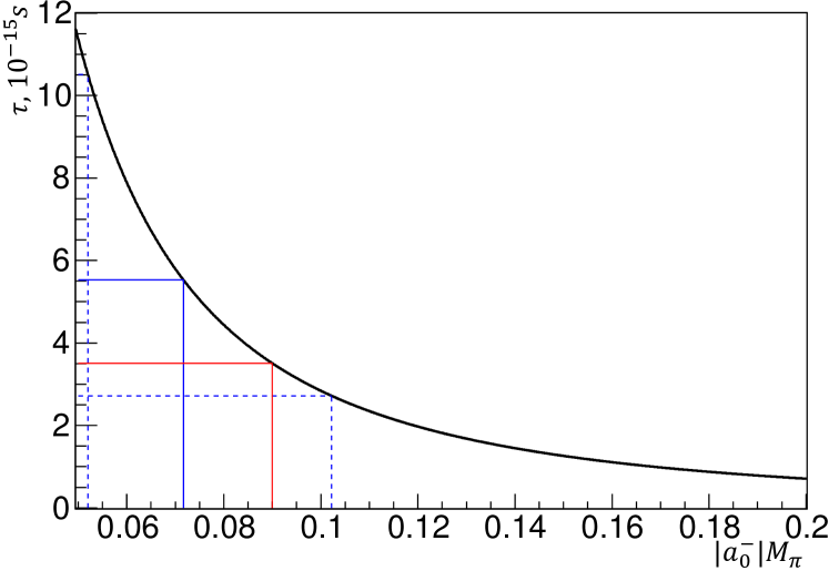
Figure 17: Ground state $A_{\pi K}$ lifetime $\tau_{1S}$ versus $a_{0}^{-}$ form $Q$ analysis. Experimental results (blue lines) are compared to the theoretical prediction (red lines).

All theoretical predictions are compatible with the measured value taking into account the experimental precision. The main contribution to the experimental uncertainty comes from statistics. As shown in GORC16 , the number of $\pi K$ atoms detected per time unit would be increased by a factor of 30 to 40, if the DIRAC experiment could exploit the CERN SPS 450 $\text{GeV}/c$ proton beam.Under these conditions, the statistical precision of $a_{0}^{-}$ will be around 5% for a single run period.

VIII Conclusion

The DIRAC Collaboration published the observation of $\pi^{-}K^{+}$ and $\pi^{+}K^{-}$ atoms ADEV16 . These atoms were generated by the 24 $\text{GeV}/c$ protons of the CERN PS in Ni and Pt targets, where a part of them broke up, yielding $\pi^{-}K^{+}$ and $\pi^{+}K^{-}$ atomic pairs. In the present article, the breakup probabilities for each atom type and each target are determined by analyzing atomic and free $\pi K$ pairs. By means of these probabilities, the lifetime of the $\pi K$ atom in the ground state is evaluated, $\tau_{\text{tot}}=\left.(5.5^{+5.0}_{-2.8}\right|_{\text{tot}})\cdot 10^{-15}$ s, and the S-wave isospin-odd $\pi K$ scattering length deduced, $\left|a_{0}^{-}\right|=\frac{1}{3}\left|a_{1/2}-a_{3/2}\right|=\left.(0.072^{+0.031}_{-0.020}\right|_{\text{tot}})M_{\pi}^{-1}$. The measured $a_{0}^{-}$ value is compatible with our previous less precise result ADEV14 and with theoretical results calculated in ChPT, LQCD and in a dispersive framework using Roy-Steiner equations SCHW04 ; BUET04 ; WEIN66 ; Gasser85 ; BERN91 ; KUBI02 ; BIJN04 ; JANO14 ; BEAN06 ; Fu12 ; Sasaki14 .

On the basis of the statistically significant observation of $\pi K$ atoms ADEV16 , DIRAC presents a measurement of the $\pi K$ atom lifetime and the corresponding fundamental $\pi K$ scattering length.

References

- (1) B. Adeva et al., Phys. Rev. Lett. 117 (2016) 112001.
- (2) J.R. Bateley et al., Eur. Phys. J. C64 (2009) 589.
- (3) J.R. Bateley et al., Eur. Phys. J. C70 (2010) 635.
- (4) B. Adeva et al., Phys. Lett. B 704 (2011) 24.
- (5) S.M. Bilen’kii et al., Yad. Fiz. 10 (1969) 812; Sov. J. Nucl. Phys. 10 (1969) 469.
- (6) J. Schweizer, Phys. Lett. B 587 (2004) 33; Eur. Phys. J. C 36 (2004) 483.
- (7) P. Buettiker, S. Descotes-Genon and B. Moussallam, Eur. Phys. J. C33 (2004) 409.
- (8) S. Weinberg, Phys. Rev. Lett. 17 (1966) 616.
- (9) J. Gasser and H. Leutwyler, Nucl. Phys. B 250 (1985) 465.
-
(10)
V. Bernard, N. Kaiser and Ulf-G. Meissner, Phys. Rev. D43 (1991) 2757;
V. Bernard, N. Kaiser and Ulf-G. Meissner, Nucl. Phys. B357 (1991) 129. - (11) B. Kubis and Ulf-G. Meissner, Phys. Lett. B 529 (2002) 69.
- (12) J. Bijnens, P. Dhonte and P. Talavera, J. High Energy Phys. 0405 (2004) 036.
- (13) T. Janowski et al., PoS LATTICE2014 (2015) 080.
- (14) S.R. Beane, et al., Phys. Rev. D 74 (2006) 114503.
- (15) Z. Fu, Phys. Rev. D 85 (2012) 074501.
- (16) K. Sasaki, N. Ishizuka, M. Oka, T. Yamazaki, Phys. Rev. D 89 (2014) 054502.
- (17) L. Nemenov, Yad. Fiz. 41 (1985) 980; Sov. J. Nucl. Phys. 41 (1985) 629.
- (18) L. Afanasyev and A.V. Tarasov, Yad. Fiz. 59 (1996) 2212; Phys. Atom. Nucl. 59 (1996) 2130.
- (19) L. Afanasyev et al., Phys. Lett. B 308 (1993) 200.
- (20) L. Afanasyev et al., Phys. Lett. B 338 (1994) 478.
- (21) B. Adeva et al., J. Phys. G: Nucl. Part. Phys. 30 (2004) 1929.
- (22) B. Adeva et al., Phys. Lett. B 619 (2005) 50.
- (23) B. Adeva et al., Phys. Lett. B 751 (2015) 12.
- (24) B. Adeva et al., Phys. Lett. B 674 (2009) 11.
- (25) B. Adeva et al., Phys. Lett. B 735 (2014) 288.
- (26) O. Gorchakov et al., Yad. Fiz. 63 (2000) 1936; Phys. At. Nucl. 63 (2000) 1847.
- (27) O. Gorchakov and L. Nemenov, J. Phys. G: Nucl. Part. Phys. 43 (2016) 095004.
- (28) B. Adeva et al., Nucl. Instr. Meth. A 839 (2016) 52.
- (29) O. Gorchakov and A. Kuptsov, DN (DIRAC Note) 2005-05; cds.cern.ch/record/1369686.
- (30) O. Gorchakov, DN 2005-23; cds.cern.ch/record/1369668.
- (31) M. Pentia et al., Nucl. Instr. Meth. A 795 (2015) 200.
- (32) G. Gamov, Z. Phys. 51 (1928) 204.
- (33) A. Sommerfeld, Atombau und Spektrallinien, F. Vieweg & Sohn (1931).
- (34) A.D. Sakharov, Sov. Phys. Usp. 34 (1991) 375.
-
(35)
L. Afanasyev and O. Voskresenskaya, Phys. Lett. B 453 (1999) 302;
L. Afanasyev, O. Voskresenskaya and V. Yazkov, Communication JINR P1-97-306 Dubna 1997. - (36) R. Lednicky, J. Phys. G: Nucl. Part. Phys. 35 (2008) 125109.
- (37) R. Lednicky, DN 2012-05; cds.cern.ch/record/1475781.
- (38) A. Kotsinian, preprint EFI-400 (7) Erevan 1980.
- (39) L.S. Dulian and A.M. Kotsinian, Yad. Fiz. 37 (1983) 137; Sov. J. Nucl. Phys. 37 (1983) 78.
- (40) S. Mrówczyński, Phys. Rev. A 33, 1549 (1986).
-
(41)
S. Mrówczyński, Phys. Rev. D 36 (1987) 1520;
K.G. Denisenko and S.Mrówczyński, Phys. Rev. D 36 (1987) 1529. - (42) L. Afanasyev, A. Tarasov and O. Voskresenskaya, Phys. Rev. D 65 (2002) 096001.
- (43) T.A. Heim et al., J. Phys. B: At. Mol. Opt. Phys. 33 (2000) 3583.
- (44) T.A. Heim et al., J. Phys. B: At. Mol. Opt. Phys. 34 (2001) 3763.
- (45) M. Schumann, et al., J. Phys. B: At. Mol. Opt. Phys. 35 (2002) 2683.
- (46) M. Zhabitsky, DN 2014-06; cds.cern.ch/record/1987122.
- (47) A.V. Tarasov and I.U. Khristova, JINR-P2-91-10 Dubna 1991.
- (48) O. Voskresenskaya, S.R. Gevorkyan and A.V. Tarasov, Phys. At. Nucl. 61 (1998) 1517.
- (49) L. Afanasyev, A. Tarasov and O. Voskresenskaya, J. Phys. G 25 B7 (1999) 224.
- (50) D.Yu. Ivanov and L. Szymanowski, Eur. Phys. J. A5 (1999) 117.
-
(51)
T.A. Heim et al., Proc. Workshop on Hadronic Atoms HadAtom01 Bern 2001 13;
arXiv:hep-ph/0112293. - (52) Z. Halabuka et al., Nucl. Phys. B 554 (1999) 86.
- (53) M.V. Zhabitsky, Phys. At. Nucl. 71 (2008) 1040.
- (54) O. Voskresenskaya, J. Phys. B: At. Mol. Opt. Phys. 36 (2003) 3293.
- (55) L. Afanasyev et al., J. Phys. B: At. Mol. Opt. Phys. 37 (2004) 4749.
- (56) M. Zhabitsky, DN 2007-11; cds.cern.ch/record/1369651.
- (57) B. Adeva et al., Addendum to the DIRAC Proposal CERN–SPSC–2004–009 SPSC-P-284 Add. 4; http://cds.cern.ch/record/729809.
-
(58)
DIRAC Collaboration,
dirac.web.cern.ch/DIRAC/offlinedocs/Userguide.html. - (59) A. Benelli and V. Yazkov, DN 2016-01; cds.cern.ch/record/2137645.
-
(60)
O. Gorchakov, DN 2009-10; cds.cern.ch/record/1369625;
DN 2009-08; cds.cern.ch/record/1369627;
DN 2009-02; cds.cern.ch/record/1369633;
DN 2008-09; cds.cern.ch/record/1369636. - (61) B. Adeva, A. Romero and O. Vazquez Doce, DN 2005-16; cds.cern.ch/record/1369675.
- (62) J. Beringer et al. (Particle Data Group), Phys. Rev. D 86 (2012) 010001.
- (63) B. Adeva et al., CERN-EP-2017-137; cds.cern.ch/record/2268734.
- (64) P. Doskarova and V. Yazkov, DN 2013-05; cds.cern.ch/record/1628541.
- (65) A. Benelli and V. Yazkov, DN 2009-07; cds.cern.ch/record/1369628.
- (66) V. Yazkov and M. Zhabitsky, DN 2013-06; cds.cern.ch/record/1628544.
- (67) O. Gorchakov, DN 2007-04; cds.cern.ch/record/1369657.
- (68) A. Benelli and V. Yazkov, DN 2012-04; cds.cern.ch/record/1475780.
- (69) A. Benelli and V. Yazkov, DN 2016-02; cds.cern.ch/record/2137799.
- (70) A. Benelli and V. Yazkov, DN 2016-03; cds.cern.ch/record/2207225.
- (71) O. Gorchakov, DN 2010-01; cds.cern.ch/record/1369624.
- (72) D. Drijard and M. Zhabitsky, DN 2008-07; cds.cern.ch/record/1367888.
- (73) V. Yazkov and M. Zhabitsky, DN 2016-06; cds.cern.ch/record/2252375.