Real eigenvalues in the non-Hermitian Anderson model

Ilya Goldsheidlabel=e1]i.goldsheid@qmul.ac.uk [ School of Mathematical Sciences,
Queen Mary University of London,
London E1 4NS,
United Kingdom.
   Sasha Sodinlabel=e2]a.sodin@qmul.ac.uk [ School of Mathematical Sciences,
Queen Mary University of London,
London E1 4NS,
United Kingdom
&
School of Mathematical Sciences,
Tel Aviv University,
Tel Aviv, 69978,
Israel.
Queen Mary, University of London\thanksmarkm1 & Tel Aviv University\thanksmarkm2
Abstract

The eigenvalues of the Hatano–Nelson non-Hermitian Anderson matrices, in the spectral regions in which the Lyapunov exponent exceeds the non-Hermiticity parameter, are shown to be real and exponentially close to the Hermitian eigenvalues. This complements previous results, according to which the eigenvalues in the spectral regions in which the non-Hermiticity parameter exceeds the Lyapunov exponent are aligned on curves in the complex plane.

,
47B80,
47B36,
Non-Hermitian,
Anderson model,
random Schrödinger,
keywords:
[class=MSC]
keywords:
\arxiv

arXiv:1707.02181 \startlocaldefs \endlocaldefs

and

t2Supported in part by the European Research Council starting grant 639305 (SPECTRUM) and by a Royal Society Wolfson Research Merit Award.

1 Introduction and the main result

Let $v_{1},v_{2},\cdots$ be independent, identically distributed random variables (potential) and let $g$ be a real parameter, $g\geq 0$. Consider the $N\times N$ random matrix

$$H_{N}(g)=\left(\begin{array}[]{ccccccc}v_{1}&e^{-g}&0&0&\cdots&0&e^{g}\\ e^{g}&v_{2}&e^{-g}&0&\cdots&0&0\\ 0&e^{g}&v_{3}&e^{-g}&\cdots&0&0\\ &&&\ddots&&&\\ &&&&\ddots&&\\ 0&0&0&0&&v_{N-1}&e^{-g}\\ e^{-g}&0&0&0&\cdots&e^{g}&v_{N}\end{array}\right)$$ (1.1)

Non-Hermitian matrices of the form (1.1) were introduced and studied by Hatano and Nelson [21, 22] to describe the reaction of an Anderson-localised quantum particle on a ring to a constant imaginary vector field. For $g=0$, the matrix $H_{N}=H_{N}(0)$ is Hermitian, and the eigenvalues are real. For $g>0$, the eigenvalues are not necessarily real. The numerical studies of Hatano and Nelson (carried out for the case when the $v_{j}$ have the uniform $[-1,1]$ distribution) suggest that there exist critical values $\overline{g}_{\textrm{cr}}>\underline{g}_{\textrm{cr}}>0$ such that the following holds:

  1. (a)

    For $0\leq g<\underline{g}_{\textrm{cr}}$, all the eigenvalues of $H_{N}(g)$ are real;

  2. (b)

    for $g\in(\underline{g}_{\textrm{cr}},\overline{g}_{\textrm{cr}})$, some of the eigenvalues remain real, while others align along a smooth curve in the complex plane;

  3. (c)

    essentially all eigenvalues move out of the real axis when $g>\overline{g}_{\textrm{cr}}$.

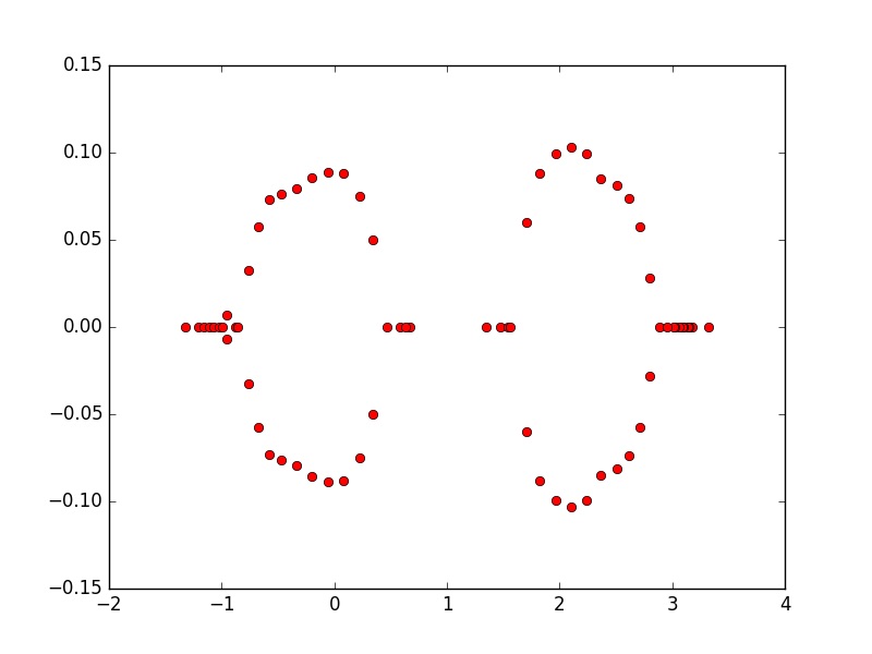
A variant of this numerical experiment in the regime (b) is depicted on Figure 1. These observations, and especially (b) and (c), were supported by the subsequent analysis performed on the physical level of rigour; see especially [7, 8, 11, 35]. We refer to these works and also to [28] and references therein for a discussion of the properties of the (left and right) eigenvectors of $H_{N}(g)$, and for extensions to the strip and to higher dimension, which will mostly remain outside the scope of this paper (see however Section 6).

In the mathematical works [16, 17, 18] of Khoruzhenko and the first author it was shown that the behaviour of the eigenvalues depends crucially on the Lyapunov exponent $\gamma(E)$ associated to the Hermitian operator (see Section 2, equation (2.2)). Let us label the algebraic spectrum of $H_{N}(g)$ $\{\lambda_{1}(g),\cdots,\lambda_{N}(g)\}$ so that each $\lambda_{j}(g)$ is a continuous function of $g$, and $\lambda_{1}(0)\geq\cdots\geq\lambda_{N}(0)$ (cf. Lemma 2.3 below).

Fix $j$; for $g=0$ the eigenvalue $\lambda_{j}(0)$ lies on the real axis. It was shown in [16, 17] that for $g<\gamma(\lambda_{j}(0))$ the eigenvalue $\lambda_{j}(g)$ remains in the vicinity of the real axis (i.e. it lies in the strip $|\Im\lambda|<\epsilon$, provided that $N\geq N_{0}(\epsilon)$), whereas for $g>\gamma(\lambda_{j}(0))$ it escapes to certain polynomial curves $\Gamma_{g}^{(N)}$ in the complex plane. These statements hold simultaneously for all the eigenvalues $\lambda_{j}(g)$ on an event of asymptotically full probability. As $N\to\infty$, $\Gamma_{g}^{(N)}$ converges to the curve $\Gamma_{g}=\{z\in\mathbb{C}\,\mid\,\gamma(z)=g\}$.

\floatbox

[\capbeside\thisfloatsetupcapbesideposition=right,center,capbesidewidth=5cm]figure[\FBwidth] Refer to caption

Figure 1: A realisation of the spectrum for a variant of (1.1) with a $2$-periodic background (cf. Remark 1.3); $N=70$ and $g=.08\in(\underline{g}_{\textrm{cr}},\overline{g}_{\textrm{cr}})$. The axis is split in 5 intervals. On the odd ones, the Lyapunov exponent is $\geq.08$; on the even ones, it is $\leq.08$.

In [18], these results were extended to a wide class of deterministic potentials, under the mild assumption of existence of the integrated density of states $\mathcal{N}(E)$. Under this assumption, one defines the Lyapunov exponent via the Thouless formula

$$\gamma(E)=\int\log|E-E^{\prime}|\,d\mathcal{N}(E^{\prime})~{}.$$

In the case of stationary random sequences, this definition coincides with the usual one, given in (2.2).

Moreover, it was shown in [18] that the eigenvalues near the curves $\Gamma_{g}$ boast regular behaviour on a local scale: after re-scaling the eigenvalues near a fixed $z\in\Gamma_{g}$ by the mean (complex) spacing, these align, in the large $N$ limit, on an arithmetic progression.

Consequently, the critical values should be given by the formulæ

$$\underline{g}_{\textrm{cr}}=\min\{\gamma(E)\,\mid\,E\in\mathcal{S}\}~{},\quad\overline{g}_{\textrm{cr}}=\max\{\gamma(E)\,\mid\,E\in\mathcal{S}\}~{},$$

where $\mathcal{S}$ is the support of the limiting eigenvalue distribution of $H_{N}(0)$ (i.e. the support of the integrated density of states $\mathcal{N}(E)$ defined in (1.3), or equivalently the essential spectrum of the infinite-volume self-adjoint operator).

The results proved in [16, 17, 18] provide a detailed statistical description of the behaviour of the eigenvalue $\lambda_{j}(g)$ for $g>\gamma(\lambda_{j}(0))$, both in the global and the local limiting regime; thus one has a complete description of the regime (c), and a partial one – of (b).

The description of the behaviour for $g<\gamma(\lambda_{j}(0))$ remained incomplete. In fact, neither the rigorous analysis of [16, 17, 18] nor the heuristic arguments of [7, 8, 11, 35] provide an indication on whether these eigenvalues are truly real (as suggested by computer simulations such as Figure 1), or they may have a non-zero but asymptotically vanishing imaginary part.

To the best of our knowledge, no progress on this question has been made since the work [18] had been published. We are also not aware of any previous analysis of the spacings between these eigenvalues (the local regime).

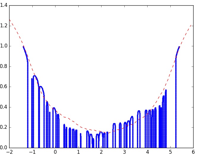
In this work we provide a reasonably complete description of the regime $\gamma(\lambda_{j}(0))>g$, thus settling these two questions. We prove that in the case of (1.1) with independent, identically distributed potential the corresponding non-Hermitian eigenvalues $\lambda_{j}(g)$ do in fact remain on the real axis, and, moreover, they are exponentially close to the Hermitian eigenvalues $\lambda_{j}(0)$. In other words, if $j$ is fixed and $g$ varies from 00 to $\infty$, the eigenvalue $\lambda_{j}(g)$ remains real and exponentially close to $\lambda_{j}(0)$ for $g\leq\gamma(\lambda_{j}(0))-\epsilon$ (where $\epsilon>0$ is arbitrary small, and $N\geq N_{0}(\epsilon)$). This complements the result of [18], according to which $\lambda_{j}(g)$ aligns near $\Gamma_{g}$ for $g\geq\gamma(\lambda_{j}(0))+\epsilon$. See Figure 2 for an illustration.

\floatbox

[\capbeside\thisfloatsetupcapbesideposition=right,center,capbesidewidth=3cm]figure[\FBwidth] Refer to caption

Figure 2: The curves connecting the points $(\lambda_{j}(g),g)\in\mathbb{R}^{2}$ with $\lambda_{j}(g)\in\mathbb{R}$, for $N=70$ and $v_{j}\sim\operatorname{Unif}[0,4]$. In the large $N$ limit, the upper envelope of these curves converges to the graph of $\gamma(E)$ on $\mathcal{S}$. Note that the curves are almost vertical.

In contrast to the potential-theoretic approach of [18], our arguments are based on the properties of products of random matrices.

Theorem 1.

Assume that $(v_{j})$ is a sequence of i.i.d. random variables and that $|v_{1}|\leq A<\infty$ almost surely. Then for any $\epsilon>0$

$$\mathbb{P}\Big{\{}\text{for all $1\leq j\leq N$ and $g\in[0,\gamma(\lambda_{j}(0))-\epsilon]$ one has:}\,\,\,\lambda_{j}(g)\in\mathbb{R}\Big{\}}\underset{N\to\infty}{\longrightarrow}1$$

and moreover there exists $c=c(\epsilon)>0$ such that

$$\mathbb{P}\Big{\{}\forall j\,\,\,\forall g\in[0,\gamma(\lambda_{j}(0))-\epsilon]:\,\,\,\lambda_{j}(g)\in(\lambda_{j}(0)-e^{-cN},\lambda_{j}(0)+e^{-cN})\Big{\}}\underset{N\to\infty}{\longrightarrow}1~{}.$$
Remark 1.1.

The first part of the theorem is essentially equivalent to the following statement: if $I$ is an interval, then for any $\epsilon>0$

$$\lim_{N\to\infty}\mathbb{P}\left\{\text{for all $\lambda_{j}(0)\in I$ and all $g\leq\inf_{E\in I}\gamma(E)-\epsilon$ one has $\lambda_{j}(g)\in I$}\right\}=1~{}.$$
Remark 1.2.

Without invoking new ideas, the theorem can be shown to hold under the weaker assumption $\mathbb{E}|v_{1}|^{\eta}<\infty$ for some $\eta>0$. We restrict ourselves to the case of bounded random variables, to keep the argument reasonably short. On the other hand, we do insist on avoiding any regularity assumptions on the potential.

Remark 1.3.

Only minor adjustments in the argument are required to consider a variant of the model in which $v_{j}$ is replaced with $v_{j}+a_{j}$, where $(a_{j})$ is a non-random periodic sequence. For cosmetic reasons, we chose to depict this variant in Figure 1, which we included for illustration only.

Remark 1.4.

Similarly to [17] and in contrast to [18] we assume that $(v_{j})$ is an i.i.d. sequence. While we do not expect the conclusion of the theorem to hold in the generality of [18], additional special cases such as operators with almost-periodic potentials merit further consideration.

The theorem implies that the local eigenvalue statistics of $H_{N}(g)$ in the regime $g<\gamma(\lambda_{j}(0))$ are the same as for the Hermitian operator $H_{N}(0)$.

Corollary 1.5.

In the setting of Theorem 1, assume that for $g=0$

$$\sum_{j=1}^{N}\delta_{(\lambda_{j}(g)-E)N\rho}\,\,\overset{\operatorname{distr}}{\longrightarrow}\,\,\text{standard Poisson process}$$ (1.2)

for some $E\in\mathbb{R}$, $\rho>0$, as $N\to\infty$. Then (1.2) holds for all $0\leq g<\gamma(E)$.

In the Hermitian case $g=0$, a limit theorem of the form (1.2) was first proved by Molchanov [27] for a class of (continual) one-dimensional Hermitian random Schrödinger operators. An extension to higher-dimensional operators in the regime of Anderson localisation was proved by Minami [26]; his result implies that (1.2) holds (for $g=0$) if the cumulative distribution function of $v_{1}$ is uniformly Lipschitz, with

$$\rho=\rho(E)=\mathcal{N}^{\prime}(E)~{},\quad\mathcal{N}(E)=\lim_{N\to\infty}\frac{1}{N}\#\{\lambda_{j}(0)<E\}~{}.$$ (1.3)

The existence of the density of states $\rho(E)=\mathcal{N}^{\prime}(E)$ (in the sense of Radon) in this situation follows from an argument of Wegner [34].

Recently, Bourgain showed [5] for the one-dimensional case that the density of states exists (and in fact $\mathcal{N}$ is $C^{\infty}$ smooth) whenever the cumulative distribution function of $v_{1}$ is uniformly Hölder continuous of some order $\nu>0$. In [6], he showed that (1.2) holds (for $g=0$) under the same assumptions, for the case of Dirichlet boundary conditions (i.e. the top-right and bottom-left corner matrix elements are set to zero). The argument of [6] can be adjusted to periodic boundary conditions (i.e. to $H_{N}(0)$). Combining this with Corollary 1.5, we obtain that, under the same assumption, (1.2) also holds for all $g<\gamma(E)$ (at least, if $v_{1}$ is bounded almost surely).

The logical structure of the paper

The key ingredient in the proof of Theorem 1 is a uniform lower bound on the spectral radius of the transfer matrices associated with the Hermitian matrices $H_{N}(0)$, outside exponentially small neighbourhoods of the bands. This bound, possibly of independent interest, is stated as Proposition 3.1 in Section 3.1, where we also provide its proof. In Section 3.2 we use it to prove Theorem 1.

The proof of Proposition 3.1 makes use of several facts from the theory of random matrix products: particularly, a large deviation bound for the norm (Lemma 2.1) and a comparison between the norm and the spectral radius (Lemma 2.2). While such statements are well known (the former goes back to the work of Le Page [24], and the latter – to the work of Guivarc’h [20] and Reddy [30]), the form in which we found them (and particularly the latter one) in the literature is somewhat weaker than what is needed for our purposes. Therefore we develop, in Sections 4 and 5, an approach (close in spirit to the article [32] of Shubin–Vakilian–Wolff and to unpublished work of the first author on the central limit theorem for eigenvalues of random matrix products) which allows us to re-prove these statements in the required form. Two other important ingredients of the proof of Proposition 3.1 are Lemmata 2.5 and 2.4, due to Bourgain [6] and Le Page [25], respectively. The latter lemma lies in the field of random matrix products, and in the short Section 5.2, we deduce it from Lemma 2.1.

In Section 2, we formulate the definitions and the lemmata required to state and prove Proposition 3.1. Possible generalisations and extensions of Theorem 1 are discussed in Section 6.

2 Preliminaries

Transfer matrices

Let $E\in\mathbb{R}$. For $N=1,2,\cdots$, define

$$\Phi_{N}(E)=T_{N}(E)\cdots T_{2}(E)T_{1}(E)~{},$$

where

$$T_{j}(E)=\left(\begin{array}[]{cc}E-v_{j}&-1\\ 1&0\end{array}\right)\in SL_{2}(\mathbb{R})~{}.$$ (2.1)

More generally, one may consider the matrices $T_{j}(z)$ and $\Phi_{N}(z)$ for $z\in\mathbb{C}$. As usual, $\Phi_{N}(z)$ is associated to the formal solutions $\psi$ of the equation

$$\psi_{j-1}+v_{j}\psi_{j}+\psi_{j+1}=z\psi_{j}~{},\quad j\geq 1$$

as follows:

$$\Phi_{N}\begin{pmatrix}\psi_{1}\\ \psi_{0}\end{pmatrix}=\begin{pmatrix}\psi_{N+1}\\ \psi_{N}\end{pmatrix}~{}.$$

Denote

$$\gamma(E)=\lim_{N\to\infty}\frac{1}{N}\mathbb{E}\log\|\Phi_{N}(E)\|~{}.$$ (2.2)

According to a result of Furstenberg and Kesten [14], for any stationary ergodic sequence $v=(v_{j})$, the following equality holds with probability one for any (fixed) $E$:

$$\lim_{N\to\infty}\frac{1}{N}\log\|\Phi_{N}(E)\|=\gamma(E)~{}.$$ (2.3)

We emphasise that (2.3) does not hold simultaneously for all $E$ (see [15]); in fact, in the i.i.d. case the left-hand side of (2.2) vanishes on a dense random subset of $\mathcal{S}$.

A fundamental fact which is crucial for our considerations is the positivity of the Lyapunov exponent: in the i.i.d. case, Furstenberg’s theorem [13] implies that $\gamma(E)>0$ for all $E\in\mathbb{R}$. (Formally, we use the quantitative version (4.5) of this fact.)

Large deviations

Large deviations bounds for the norm of a random matrix product go back to the work of Le Page [24]. There are numerous extensions, see particularly the recent work [31], where a large deviation principle was obtained, and references therein. We need the following upper bound, close to the original work of Le Page; a proof is provided in Section 5.1.

Lemma 2.1 (Le Page).

If $\mathbb{E}|v_{1}|^{\eta}<\infty$ for some $\eta>0$, then for any $R>0$ there exist $C,c>0$ such that for $\epsilon\in(0,1/e)$ and $|E|\leq R$

$$\mathbb{P}\left\{\left|\frac{1}{N}\log\|\Phi_{N}(E)\|-\gamma(E)\right|\geq\epsilon\right\}\leq\left(C\log\frac{1}{\epsilon}\right)\exp\left[-\frac{c\epsilon^{2}N}{\log\frac{1}{\epsilon}}\right]~{}.$$ (2.4)

Spectral radius

We shall use the following lemma, which is a variant of the results proved by Guivarc’h [20, §2.4] and by Reddy [30]. We provide a proof in Section 4.3. For a matrix $\Phi$ we denote by $\rho(\Phi)$ its spectral radius.

Lemma 2.2.

If $\mathbb{E}|v_{1}|^{\eta}<\infty$ for some $\eta>0$, then for any $R>0$ there exist $B,B^{\prime}>0$ and $b,b^{\prime}>0$ such that

$$\sup_{|E|\leq R}\mathbb{P}\left\{\rho(\Phi_{N}(E))\leq\delta\|\Phi_{N}(E)\|\right\}\leq B\delta^{b}+B^{\prime}e^{-b^{\prime}N}~{},\quad 0\leq\delta\leq 1~{}.$$

Bands and gaps

Consider the transfer matrices corresponding to the potential $(v_{j})$ (in this paragraph the potential does not have to be random). The set of $E$ such that $\rho(\Phi_{N}(E))=1$ consists of $N$ disjoint intervals (bands); we denote their interiors, numbered from the rightmost to the leftmost, $I_{1},\cdots,I_{N}$. Denote

$$\mathbb{R}=G_{0}\uplus I_{1}\uplus G_{1}\uplus I_{2}\uplus\cdots\uplus I_{N}\uplus G_{N}~{},$$

where the $G_{j}$ (the closures of the gaps) are also ordered from right to left.

The eigenvalues of the periodic operator $H_{N}(0)$ are exactly the points $E$ at which $1$ is an eigenvalue of $\Phi_{N}(E)$. These are exactly the edges of the gaps $G_{0},G_{2},\cdots$ with even indices. This fact admits the following generalisation to the non-Hermitian case (cf.  [17, 18]):

Lemma 2.3 ([18, Lemma 4.1]).

The eigenvalues of $H_{N}(g)$ are the points $z\in\mathbb{C}$ such that $e^{Ng}$ is an eigenvalue of $\Phi_{N}(z)$.

Hölder continuity of the Lyapunov exponent

The local Hölder continuity of the Lyapunov exponent goes back to the work of Le Page [25]. We need the following version, proved in [9] and, by different arguments, in [32, 4]; for the sake of unity of argument, we provide a proof in Section 5.2.

Lemma 2.4 (Le Page).

If $v_{j}$ are independent, identically distributed with $\mathbb{E}|v_{1}|^{\eta}<\infty$ for some $\eta>0$, then the Lyapunov exponent $\gamma(E)$ associated to the sequence $T_{N}(E)$ is uniformly Hölder continuous on any compact interval.


Gaps between the eigenvalues

Lemma 2.5 (Bourgain [6]).

If $v_{j}$ are independent, identically distributed with $\mathbb{E}|v_{1}|^{\eta}<\infty$ for some $\eta>0$, then for any $R>0$ there exists $K>0$ such that

$$\mathbb{P}\left\{\min_{\text{$\lambda\neq\lambda^{\prime}$--eigenvalues of $H_{N}$ in $[-R,R]$}}|\lambda-\lambda^{\prime}|<N^{-K}\right\}=0~{}.$$
Remark 2.6.

In the work [6] the lemma is proved for Dirichlet rather than periodic boundary conditions, and only for the case of Bernoulli potential. However, the argument presented there applies equally well in the current setting.

Remark 2.7.

The argument in [6] relies on Anderson localisation. On the other hand, if the cumulative distribution function of $v_{1}$ is uniformly Hölder of order $\nu>1/2$, the conclusion of the lemma also follows from the Minami estimate, see [26] and further [10, 19]. Thus, for such potentials, the conclusion of Theorem 1 is established using fixed-energy arguments only.

3 Proof of the main result

3.1 The key technical statement

Let $c>0$ be a sufficiently small constant, to be chosen later. For a gap $G_{j}=[a_{j},b_{j}]$, denote

$$G_{j}^{+,c}=[b_{j}-e^{-cN},b_{j}]~{},\quad G_{j}^{-,c}=[a_{j},a_{j}+e^{-cN}]~{}.$$

The following proposition provides uniform control of the transfer matrices outside exponentially small neighbourhoods of the bands. It is the key ingredient in the proof of the main theorem. Having in mind possible additional applications (in the Hermitian and non-Hermitian setting), we formulate it as an independent statement.

Proposition 3.1.

Let $v_{j}$ be i.i.d. with $|v_{1}|\leq A$ for some $A>0$. Then for any $\epsilon>0$

$$\lim_{N\to\infty}\mathbb{P}\left\{\forall 1\leq j<N\,\,\,\max_{E\in G_{j}}\frac{1}{N}\log\rho(\Phi_{N}(E))\geq\max_{E\in G_{j}}\gamma(E)-\epsilon\right\}=1~{}.$$ (3.1)

In addition, if $c>0$ is small enough and $\mathfrak{s}\in\{+,-\}$,

$$\lim_{N\to\infty}\mathbb{P}\left\{\forall 1\leq j<N\,\,\,\max_{E\in G_{j}^{\mathfrak{s},c}}\frac{1}{N}\log\rho(\Phi_{N}(E))\geq\max_{E\in G_{j}}\gamma(E)-\epsilon\right\}=1~{}.$$ (3.2)
Proof.

As customary, we denote $\lfloor x\rfloor=\max_{n\leq x}n$ and $\lceil y\rceil=\min_{n\geq x}n$.

If $|v_{1}|\leq A<\infty$ almost surely, then $\|H_{N}(0)\|\leq 2+A$. Let $(E_{l})_{l=1}^{\lfloor e^{cN}\rfloor}$ be a sequence of equally spaced points with $E_{1}=-3-A$ and $E_{\lfloor e^{cN}\rfloor}=3+A$.

The large deviation estimate of Lemma 2.1 allows to bound the norm of the transfer matrix from below, outside an event of small probability. Formally, for any $E_{l}\in[-3-A,3+A]$, we have

$$\mathbb{P}\left\{\,\|\Phi_{N}(E_{l})\|\leq e^{N(\gamma(E_{l})-\frac{\epsilon}{4})}\right\}\leq B_{1}e^{-b_{1}N},$$

where $B_{1}$ and $b_{1}$ do not depend on $E_{l}\in[-3-A,3+A]$.

In turn, Lemma 2.2 allows to compare the spectral radius with the norm: taking $\delta=e^{-N\frac{\epsilon}{4}}$ in the lemma, we obtain for any $E_{l}$:

$$\mathbb{P}\left\{\,\rho(\Phi_{N}(E_{l}))\leq e^{-N\frac{\epsilon}{4}}\|\Phi_{N}(E_{l})\|\right\}\leq Be^{-Nb\frac{\epsilon}{4}}+B^{\prime}e^{-b^{\prime}N}\leq Ce^{-\bar{b}N},$$

where $C>0$ and $\bar{b}>0$ do not depend on $E_{l}\in[-3-A,3+A]$. Hence

$$\begin{split}&\mathbb{P}\left\{\exists l:\,\,\frac{1}{N}\log\rho(\Phi_{N}(E_{l}))\leq\gamma(E_{l})-\frac{\epsilon}{2}\right\}\\ &\quad\leq e^{cN}\left[B_{1}e^{-b_{1}N}+Ce^{-\bar{b}N}\right]\leq C^{\prime}e^{-c^{\prime}N}~{},\end{split}$$

where we chose $c>0$ small enough ($c<\min(b_{1},\bar{b})$). In particular, the probability of the event

$$\Omega_{1}=\left\{\forall l\,\,\frac{1}{N}\log\rho(\Phi_{N}(E_{l}))\geq\gamma(E_{l})-\frac{\epsilon}{2}\right\}$$

tends to $1$ as $N\to\infty$.

Let $m_{j}\in G_{j}$ be such that $\max\limits_{E\in G_{j}}\gamma(E)=\gamma(m_{j})$. Denote

$$\Omega_{2}=\left\{\forall 1\leq j<N\,\exists l_{j}:\,E_{l_{j}}\in G_{j},|E_{l_{j}}-m_{j}|\leq Ce^{-cN}\right\}~{}.$$

By Lemma 2.5, no gap is exponentially short, hence each $G_{j}$ contains at least one $E_{l}$. Therefore also the probability of $\Omega_{2}$ tends to $1$, for $C>0$ large enough. Then on the event $\Omega_{1}\cap\Omega_{2}$, for sufficiently large $N$:

$$\begin{split}\forall j\quad\max_{E\in G_{j}}\frac{1}{N}\log\rho(\Phi_{N}(E))&\geq\frac{1}{N}\log\rho(\Phi_{N}(E_{l_{j}}))\\ &\geq\gamma(E_{l_{j}})-\frac{\epsilon}{2}\geq\gamma(m_{j})-\epsilon=\max_{E\in G_{j}}\gamma(E)-\epsilon~{},\end{split}$$

where we used the Hölder continuity of the Lyapunov exponent (Lemma 2.4). Similarly,

$$\forall j\quad\max_{E\in G_{j}^{\mathfrak{s},c}}\frac{1}{N}\log\rho(\Phi_{N}(E))\geq\max_{E\in G_{j}}\gamma(E)-\epsilon~{}.$$

3.2 Proof of Theorem 1

Let $\epsilon>0$. By equation (3.1) of Proposition 3.1,

$$\lim_{N\to\infty}\mathbb{P}\Big{\{}\forall 1\leq j<N\,\,\,\max_{E\in G_{j}}\frac{1}{N}\log\rho(\Phi_{N}(E))\geq\max_{E\in G_{j}}\gamma(E)-\epsilon/2\Big{\}}=1~{}.$$

On this event, we have for any $1\leq j<N$:

$$\max_{E\in G_{j}}\frac{1}{N}\log\rho(\Phi_{N}(E))\geq\max_{E\in G_{j}}\gamma(E)-\epsilon/2~{}.$$

Since $G_{2j}=[\lambda_{2j+1},\lambda_{2j}]$ (where $\lambda_{j}=\lambda_{j}(0)$; in the notation of Proposition 3.1, $a_{2j}=\lambda_{2j+1}$ and $b_{2j}=\lambda_{2j}$), we conclude the following: if, for some $g$,

$$\max(\gamma(\lambda_{2j}),\gamma(\lambda_{2j+1}))\geq g+\epsilon~{},$$

then

$$\max_{E\in G_{2j}}\frac{1}{N}\log\rho(\Phi_{N}(E))\geq(g+\epsilon/2)~{}.$$

On the other hand, $\frac{1}{N}\log\rho(\Phi_{N}(\lambda_{2j}))=\frac{1}{N}\log\rho(\Phi_{N}(\lambda_{2j+1}))=0$, hence by the intermediate value theorem there are two solutions to $\rho(\Phi_{N}(E))=e^{Ng}$ lying in $G_{j}$. By Lemma 2.3, these are exactly the eigenvalues $\lambda_{2j}(g)$ and $\lambda_{2j+1}(g)$. As to the eigenvalues $\lambda_{1}(g)$ and, for even $N$, $\lambda_{N}(g)$, these are real. Invoking the second part (3.2) of Proposition 3.1, we obtain that $|\lambda_{j}(g)-\lambda_{j}(0)|$ is exponentially small. ∎

4 On the spectral radius of transfer matrices

The ultimate goal of this section is the proof of Lemma 2.2 in Section 4.3. We start with some auxiliary statements.

Let $T_{j}=T_{j}(E)$ with $\mathbb{E}|v_{j}|^{\eta}<\infty$ for some $\eta>0$. Then $\mathbb{E}\|T_{j}\|^{\eta}<e^{A\eta}$, where $A>0$ can be chosen locally uniformly in $E$. Let $\Phi_{N}=T_{N}\cdots T_{2}T_{1}$, and further let $\Phi_{N,M}=T_{N}\cdots T_{M+1}$ for $N>M$. We use the singular value decomposition

$$\Phi_{N}=U_{N}\left(\begin{array}[]{cc}s_{N}&0\\ 0&s_{N}^{-1}\end{array}\right)V_{N}~{},\quad\Phi_{N,M}=U_{N,M}\left(\begin{array}[]{cc}s_{N,M}&0\\ 0&s_{N,M}^{-1}\end{array}\right)V_{N,M}~{},$$ (4.1)

where $s_{N},s_{N,M}\geq 1$, $U_{N},V_{N},U_{N,M},V_{N,M}\in SO(2)$. The application of singular value decomposition in the study of random matrix products goes back at least to the work of Tutubalin [33], who realised that the sequence $(U_{N})$ is approximated by a Markov chain whereas $V_{N}$ converges to a random limit. This idea plays an important rôle in our analysis as well.

4.1 A lemma in linear algebra

Denote by $uv^{*}$ the rank-one operator taking $w$ to $(w,v)u$, where $(u,v)$ is the inner product. Also, we denote by $e_{j}$ the $j$-th vector of the standard basis. Although we need the following lemma only for two-dimensional matrices, specialising the argument to this case would only obscure the idea.

Lemma 4.1.

If $u,v\in\mathbb{C}^{m}$ and $\mathfrak{h}:\mathbb{C}^{m}\to\mathbb{C}^{m}$ is a linear map such that $\|\mathfrak{h}\|\leq\frac{|(u,v)|^{2}}{9\|u\|\|v\|}$, then

$$\rho(uv^{*}+\mathfrak{h})\geq\frac{1}{2}|(u,v)|~{}.$$ (4.2)
Proof.

Let $0\leq t\leq 1$, and let $z$ be a complex number on the circle of radius $\frac{1}{2}|(u,v)|$ about $(u,v)$. We shall show that for such $t$ and $z$ the determinant $\det(z-uv^{*}-t\mathfrak{h})$ does not vanish. This will imply that the number of eigenvalues of $uv^{*}+t\mathfrak{h}$ in the disc enclosed by the circle does not change as $t$ varies from 00 to $1$. For $t=0$, the spectrum of $uv^{*}$ consists of two eigenvalues, 00 (with multiplicity $m-1$) and $(u,v)$ (with multiplicity $1$), of which the second one lies in the disk; thus also for $t=1$ there is (exactly) one simple eigenvalue in the disc, and in particular (4.2) holds.

Let us factorise

$$\det(z\mathbbm{1}-uv^{*}-t\mathfrak{h})=\det(z\mathbbm{1}-uv^{*})\,\det(\mathbbm{1}-(z\mathbbm{1}-uv^{*})^{-1}t\mathfrak{h})~{}.$$

The first term is equal to

$$z^{m-1}(z-(u,v))~{},$$

and thus does not vanish on the circle. To show that the second term does not vanish, observe that

$$\begin{split}\|(z\mathbbm{1}-uv^{*})^{-1}\|&=\|\frac{1}{z}\mathbbm{1}+\frac{1}{z}\frac{uv^{*}}{z-(u,v)}\|\leq\frac{1}{|z|}\left\{1+\frac{\|u\|\|v\|}{|z-(u,v)|}\right\}\\ &\leq\frac{2}{|(u,v)|}\frac{4\|u\|\|v\|}{|(u,v)|}=\frac{8\|u\|\|v\|}{|(u,v)|^{2}}~{},\end{split}$$

hence

$$\|(z\mathbbm{1}-uv^{*})^{-1}t\mathfrak{h}\|\leq\frac{8\|u\|\|v\|}{|(u,v)|^{2}}\frac{|(u,v)|^{2}}{9\|u\|\|v\|}=\frac{8}{9}<1~{}.$$

Corollary 4.2.

If $\Phi=U\left(\begin{array}[]{cc}s&0\\ 0&1/s\end{array}\right)V$ with $U,V\in SO(2)$ and $s\geq 3$, $|(VUe_{1},e_{1})|\geq\frac{3}{s}$, then

$$\rho(\Phi)\geq\frac{s}{2}|(VUe_{1},e_{1})|~{}.$$
Proof.

Apply the lemma to $u=Ue_{1}$, $v=V^{*}e_{1}$, observing that

$$U\left(\begin{array}[]{cc}s&0\\ 0&0\end{array}\right)V=uv^{*}$$

and

$$\|U\left(\begin{array}[]{cc}0&0\\ 0&1/s\end{array}\right)V\|=1/s~{}.\qed$$

Our goal in the remaining part of the section is to prove the estimate

$$\mathbb{P}\left\{|(V_{N}U_{N}e_{1},e_{1})|\leq\delta\right\}\leq K\delta^{\kappa}+e^{-cN}~{},$$ (4.3)

which will imply Lemma 2.2, in view of Corollary 4.2.

4.2 On an important unitary operator

For each $T\in SL_{2}(\mathbb{R})$, consider the operator $\pi(T):L_{2}(S^{1})\to L_{2}(S^{1})$, defined via

$$(\pi(T)f)(x)=f(Tx/\|Tx\|)/\|Tx\|~{}.$$

For any $T\in SL_{2}(\mathbb{R})$, $\pi(T)$ is unitary.

Lemma 4.3 (Shubin–Vakilian–Wolff [32]).

If $v_{1}$ is not almost surely equal to a constant, then there exists $a>0$ such that

$$\sup_{E}\|(\mathbb{E}\pi(T_{1}(E)))^{2}\|\leq e^{-a}<1~{}.$$ (4.4)

Denoting by $\mathbf{1}\in L_{2}(S^{1})$ the function identically equal to $1$ and parametrising the points on the circle by an argument $\theta\in[0,2\pi]$, we obtain:

$$\mathbb{E}\|\Phi_{n}(E)\|^{-1}\leq\mathbb{E}\int_{0}^{2\pi}\frac{d\theta}{2\pi}\|\Phi_{n}(E)e^{i\theta}\|^{-1}=\frac{1}{2\pi}(\mathbb{E}\pi(\Phi_{n})\mathbf{1},\mathbf{1})\leq e^{-a\lfloor\frac{n}{2}\rfloor}~{},$$ (4.5)

and in particular $\gamma\geq a/2$.

Next, by the Oseledec multiplicative ergodic theorem [29], $V_{N}$ converges almost surely to a random limit $V$. We use this fact in the following form:

Lemma 4.4.

Suppose $\mathbb{E}|v_{1}|^{\eta}<\infty$ for some $\eta>0$. Then, for any $R>0$,

$$\sup_{|E|\leq R}\mathbb{E}\|V_{N}(E)-V(E)\|\leq Be^{-bN}~{}.$$
Proof.

Let $V_{N}^{*}e_{2}=\cos\theta\,V_{N-1}^{*}e_{2}+\sin\theta\,V_{N-1}^{*}e_{1}$. Then

$$\begin{split}\|\Phi_{N}\|^{-1}&=\|\Phi_{N}V_{N}^{*}e_{2}\|=\|T_{N}\Phi_{N-1}V_{N}^{*}e_{2}\|\geq\|T_{N}\|^{-1}\|\Phi_{N-1}V_{N}^{*}e_{2}\|\\ &\geq\|T_{N}\|^{-1}\left[\cos^{2}\theta\|\Phi_{N-1}\|^{-2}+\sin^{2}\theta\|\Phi_{N-1}\|^{2}\right]^{1/2}\\ &\geq|\sin\theta|\,\|T_{N}\|^{-1}\|\Phi_{N-1}\|~{},\end{split}$$

whence

$$|\sin\theta|\leq\frac{\|T_{N}\|}{\|\Phi_{N}\|\,\|\Phi_{N-1}\|}~{},$$

and, using (4.5),

$$\mathbb{E}|\sin\theta|\leq\mathbb{E}|\sin\theta|^{\eta}\leq e^{A(R)\eta}\,B_{0}e^{-bN}~{},$$

Thus an estimate of the same form holds for $\|V_{N}-V_{N-1}\|$ in place of $|\sin\theta|$. ∎

4.3 Conclusion of the proof of Lemma 2.2

As before, we denote $\lfloor x\rfloor=\max_{n\leq x}n$ and $\lceil y\rceil=\min_{n\geq x}n$. In the notation of (4.1), Lemma 4.4 applied to the matrix products $T_{N}\cdots T_{1}$ and $T_{1}^{*}T_{2}^{*}\cdots T_{N}^{*}$ implies that for $N\geq C\log A$

$$\mathbb{E}\|V_{N}-V_{\lfloor N/2\rfloor}\|\leq e^{-b^{\prime}N}~{},\quad\mathbb{E}\|U_{N}-U_{N,\lceil N/2\rceil}\|\leq e^{-b^{\prime}N}~{}.$$ (4.6)

The matrices $V_{\lfloor N/2\rfloor},U_{N,\lceil N/2\rceil}$ are independent, therefore by an additional application of Lemma 4.4

$$\mathbb{E}\|V_{N}-\tilde{V}\|\leq e^{-b^{\prime}N}~{},\quad\mathbb{E}\|U_{N}-\tilde{U}\|\leq e^{-b^{\prime}N}~{},$$ (4.7)

where $\tilde{U},\tilde{V}\in SO(2)$ are independent random matrices sampled from the corresponding limiting distributions. To conclude the proof of Lemma 2.2, we state (and prove)

Lemma 4.5.

Assume that $\mathbb{E}|v_{1}|^{\eta}<\infty$, and that $v_{1}$ is not almost surely constant. Then for any $E$ there exist $K>0$ and $\kappa>0$ such that for any $0\leq\delta\leq 1$ and $w,w^{\prime}\in S^{1}$

$$\mathbb{P}\left\{|(U(E)w,w^{\prime})|\leq\delta\right\}\leq K\,\delta^{\kappa}~{},\quad\mathbb{P}\left\{|(V(E)w,w^{\prime})|\leq\delta\right\}\leq K\,\delta^{\kappa}~{}.$$ (4.8)

The numbers $K$ and $\kappa$ may be chosen locally uniformly in $E$.

Proof of Lemma 2.2.

Applying Lemma 4.5 with $\tilde{U}$ and $\tilde{V}$ in place of $U$ and $V$, we obtain:

$$\mathbb{P}\left\{|(\tilde{V}\tilde{U}e_{1},e_{1})|\leq\delta\right\}\leq K\,\delta^{\kappa}~{}.$$ (4.9)

Together with (4.7), this implies (4.3), which by Corollary 4.2 implies the conclusion of Lemma 2.2. ∎

Proof of Lemma 4.5.

Since we do not keep track on the dependence of the constants on $a$ (from Lemma 4.3) and $\eta$, we may assume that $a<4\eta$. Let $\mathcal{C}_{\delta}\subset S^{1}$ be a cap of angular size $\delta$. Assume: $\mathbb{E}\|T_{1}\|^{\eta}\leq e^{A\eta}$, and denote $n=\lfloor\log\frac{2(A+1)}{\delta}\rfloor$. Let us show that

$$\mathbb{P}\left\{V_{n}^{*}e_{2}\in\mathcal{C}_{\delta}\right\}\leq C\lceil\log\frac{16(A+1)}{a}\rceil e^{-\frac{an}{16}}~{}.$$ (4.10)

By an additional application of Lemma 4.4, this implies (4.8).

To prove (4.10), we start with the estimates

$$\mathbb{E}\|\Phi_{n}\|^{\eta}\leq e^{An\eta}~{},\quad\mathbb{E}\|\Phi_{n}\|^{-1}\leq(\mathbb{E}\pi(\Phi_{n})\mathbf{1},\mathbf{1})\leq 2\pi e^{-\frac{an}{2}}~{},$$

which imply that

$$\mathbb{P}\left\{e^{\frac{an}{4}}\leq\|\Phi_{n}\|\leq e^{(A+1)n}\right\}\geq 1-C_{1}e^{-\frac{an}{4}}~{}.$$

If (4.10) fails, there exists $4\leq m\leq\lceil\log\frac{16(A+1)}{a}\rceil$ such that

$$\mathbb{P}\left\{e^{\frac{ma}{16}n}\leq\|\Phi_{n}\|\leq e^{\frac{(m+1)a}{16}n}~{},\,\,\,V_{n}^{*}e_{2}\in\mathcal{C}_{\delta}\right\}\geq Ce^{-\frac{an}{16}}~{}.$$ (4.11)

Let $\tau=\max(\delta,e^{-\frac{(m+1)a}{16}n})$, let $\mathcal{C}_{\tau}\supset\mathcal{C}_{\delta}$ be a cap of size $\tau$, and let $\mathbf{1}_{\tau}$ be the indicator of $\mathcal{C}_{\tau}$. Then (still treating $e^{i\theta}$ as a vector on the circle)

$$\mathbb{E}\int_{\mathcal{C}_{\tau}}\|\Phi_{n}e^{i\theta}\|^{-1}d\theta=(\mathbb{E}\pi(\Phi_{n})\mathbf{1},\mathbf{1})\leq C_{2}e^{-\frac{an}{2}}\sqrt{\tau}~{}.$$ (4.12)

On the other hand, if

$$V_{n}^{*}e_{2}\in\mathcal{C}_{\tau}~{},\,\,\,e^{\frac{ma}{16}n}\leq\|\Phi_{n}\|\leq e^{\frac{(m+1)a}{16}n}~{},$$ (4.13)

then

$$\int_{\mathcal{C}_{\tau}}\|\Phi_{n}e^{i\theta}\|^{-1}d\theta\geq\frac{1}{C_{3}}\min(\tau,\|\Phi_{n}\|^{-2})\|\Phi_{n}\|\geq\frac{1}{C_{3}}\tau e^{\frac{(m-1)a}{16}n}~{},$$ (4.14)

therefore by (4.11)

𝒞τΦneiθ1𝑑θ1C3τΦn1C3τe(m1)a16n(the event (4.13))1C3τe(m1)a16nCean16.subscriptsubscript𝒞𝜏superscriptdelimited-∥∥subscriptΦ𝑛superscript𝑒𝑖𝜃1differential-d𝜃1subscript𝐶3𝜏delimited-∥∥subscriptΦ𝑛1subscript𝐶3𝜏superscript𝑒𝑚1𝑎16𝑛the event (4.13)1subscript𝐶3𝜏superscript𝑒𝑚1𝑎16𝑛𝐶superscript𝑒𝑎𝑛16\begin{split}\mathbb{\int}_{\mathcal{C}_{\tau}}\|\Phi_{n}e^{i\theta}\|^{-1}d\theta&\geq\frac{1}{C_{3}}\tau\|\Phi_{n}\|\geq\frac{1}{C_{3}}\tau e^{\frac{(m-1)a}{16}n}\,\,\mathbb{P}(\text{the event (\ref{eq:linv2})})\\ &\geq\frac{1}{C_{3}}\tau e^{\frac{(m-1)a}{16}n}Ce^{-\frac{an}{16}}~{}.\end{split} (4.15)

If we choose $C>C_{2}C_{3}$, the juxtaposition of (4.15) with (4.12) leads to

$$e^{-\frac{(m+1)a}{16}n}\leq\sqrt{\tau}\leq e^{-\frac{(m-1)a}{16}n}e^{\frac{an}{16}}e^{-\frac{an}{2}}~{},$$

which is a contradiction. ∎

5 Proofs of the additional lemmata

5.1 Large deviations: proof of Lemma 2.1

We suppress the dependence on the spectral parameter $E$, on which the estimates below are locally uniform. Fix $x\in S^{1}$. It will suffice to prove the following: for any $\epsilon\in(0,1/e)$

$$\mathbb{P}\left\{\left|\frac{1}{N}\log\|\Phi_{N}x\|-\gamma\right|\geq\epsilon\right\}\leq C\log\frac{1}{\epsilon}\exp\left\{-\frac{c\epsilon^{2}N}{\log\frac{1}{\epsilon}}\right\}~{}.$$

Let $x_{0}=x$, and let $x_{j+1}=T_{j+1}x_{j}/\|T_{j+1}x_{j}\|$. The vectors $x_{j}\in S^{1}$ form a Markov chain, and

$$\|\Phi_{N}x\|=\prod_{j=1}^{N}\|T_{j}x_{j-1}\|~{}.$$

Our strategy from this point (based on two arguments going back to the work of S. N. Bernstein [2, 3]) is as follows. Fix $k=\lceil\log\frac{1}{\epsilon}\rceil$, and split the product into $k$ sub-products corresponding to the different residues of $j$ modulo $k$. The terms in each sub-product are almost independent; we make them independent by restarting the Markov chain from an invariant distribution every $k$ steps. Then we obtain a bound on the positive and negative fractional moments of each sub-product, from which the desired estimate follows using the Chebyshev inequality.

Formally, for each $j$ choose (independently) a random vector on the circle, distributed according to the invariant measure of the Markov chain; denote this vector by $y_{j-k,j}$. Then set $y_{n+1,j}=T_{n+1}y_{n,j}/\|T_{n+1}y_{n,j}\|$ for $n\geq j-k$, and, finally, define $y_{j}=y_{j,j}$. Then, for each $r$, the random variables $\left\{y_{j}\,\mid\,j\in I_{r}\right\}$, where

$$I_{r}=(r+k\mathbb{Z})\cap\{1,\cdots,N\}~{},$$

are jointly independent. The vectors $y_{j}$ are close to $x_{j}$: for $j\geq k$,

$$\mathbb{E}\left\{\|x_{j}-y_{j}\|\,\mid\,v_{1},v_{2},\cdots,v_{j-k}\right\}\leq C\exp(-ck)~{},$$ (5.1)

as implied by the following consequence of Lemma 4.5:

$$\mathbb{P}\left\{V_{j,j-k}^{*}e_{2}\in\mathcal{C}_{\delta}\right\}\leq C\left[\delta^{c}+e^{-ck}\right]~{}.$$

Denote

$$A_{r}=\prod_{j\in I_{r}}\|T_{j}x_{j-1}\|~{},\quad\text{so that}\quad\|\Phi_{N}x\|=\prod_{r=1}^{k}A_{r}~{},$$

and observe that (for $0\leq p\leq 1$)

$$\|T_{j}x_{j-1}\|^{p}\leq\|T_{j}y_{j-1}\|^{p}+\|T_{j}\|^{p}\|x_{j-1}-y_{j-1}\|^{p}$$ (5.2)

whereas

$$\begin{split}\|T_{j}x_{j-1}\|^{-p}&=\|T_{j}y_{j-1}\|^{-p}+(\|T_{j}x_{j-1}\|^{-p}-\|T_{j}y_{j-1}\|^{-p})\\ &\leq\|T_{j}y_{j-1}\|^{-p}+\frac{\|T_{j}y_{j-1}\|^{p}-\|T_{j}x_{j-1}\|^{p}}{\|T_{j}y_{j-1}\|^{p}\|T_{j}x_{j-1}\|^{p}}\\ &\leq\|T_{j}y_{j-1}\|^{-p}+\|T_{j}\|^{3p}\|x_{j-1}-y_{j-1}\|^{p}~{}.\end{split}$$ (5.3)

Also observe that (for $\eta$ from the formulation of the lemma)

$$\mathbb{E}\log\|T_{j}y_{j-1}\|=\gamma~{},\quad\mathbb{E}\|T_{j}y_{j-1}\|^{\pm\eta}\leq C<\infty~{}.$$ (5.4)

From (5.1) and (5.4) we obtain that for $0<p<\min(\frac{\eta}{10},1)$

$$\begin{split}\mathbb{E}\left\{\|T_{j}x_{j-1}\|^{p}\,\mid\,v_{1},v_{2},\cdots,v_{j-k}\right\}&\leq 1+p\gamma+C(p^{2}+e^{-ck})\\ \mathbb{E}\left\{\|T_{j}x_{j-1}\|^{-p}\,\mid\,v_{1},v_{2},\cdots,v_{j-k}\right\}&\leq 1+p\gamma+C(p^{2}+e^{-ck})~{}.\end{split}$$ (5.5)

Taking the products of each of these inequalities over $j\in I_{r}$ and using the exponential Chebyshev inequality, we have:

$$\mathbb{P}\left\{\left|\log A_{r}-\gamma\#I_{r}\right|\geq\epsilon\right\}\leq\exp(-c\epsilon^{2}\#I_{r})~{},$$ (5.6)

whence Lemma 2.1 follows by the union bound. ∎

Remark 5.1.

Using a slightly longer spectral-theoretic argument, one may dispose of the logarithmic terms in (2.4).

5.2 Hölder continuity: proof of Lemma 2.4

Let $R\geq e$, $\delta\in(0,1/e]$, and $N=\lfloor\log\frac{1}{\delta}\rfloor$. By the large deviation estimate (2.4), for any $|E|,|E^{\prime}|\leq R$

$$\mathbb{P}\left\{\Big{|}\log\|\Phi_{N}(E)\|-\gamma(E)\Big{|}<\frac{\delta}{3}~{},\quad\Big{|}\log\|\Phi_{N}(E^{\prime})\|-\gamma(E^{\prime})\Big{|}<\frac{\delta}{3}\right\}\geq\frac{3}{4}~{}.$$

Next, by the assumption $\mathbb{E}|v_{1}|^{\eta}<\infty$, we have for sufficiently large $C$:

$$\mathbb{P}\left\{\|\Phi_{j}\|\geq(CR)^{j}\right\}\leq e^{-10j}~{},$$

therefore with probability $>3/4$

$$\forall 1\leq j\leq N\quad\|\Phi_{j}(E)\|,\|\Phi_{j}(E^{\prime})\|\leq(CR)^{j}~{},\quad\|\Phi_{N,j}(E)\|,\|\Phi_{N,j}(E^{\prime})\|\leq(CR)^{N-j}~{},$$

and on this event

$$\|\Phi_{N}(E)-\Phi_{N}(E^{\prime})\|\leq|E-E^{\prime}|N(CR)^{N}~{}.$$

Therefore for $|E-E^{\prime}|\leq(2CR)^{-N}=\delta^{\log(2CR)}$

$$\left|\gamma(E)-\gamma(E^{\prime})\right|\leq\delta~{},$$

as claimed. ∎

6 Outlook

Let us briefly comment on possible extensions and directions for further study.

Other potentials

As mentioned in Remark 1.4, it would be interesting to explore the counterparts of Theorem 1 for other stationary (but non-independent) potentials. It may be of independent interest to explore the counterparts of Proposition 3.1 in this setting.

Higher dimension

The arguments used in the proof of Theorem 1 can be recast into the language of resolvent estimates. In this form, they are applicable to the following higher-dimensional analogue of (1.1) acting on $\ell_{2}(\mathbb{Z}^{d}/N\mathbb{Z}^{d})$:

$$\begin{split}(H_{N,d}(g)\psi)(x)&=e^{-g}\psi(x+e_{1})+e^{g}\psi(x-e_{1})\\ &+\sum_{j=2}^{d}(\psi(x+e_{j})+\psi(x-e_{j}))+v_{x}\psi(x)~{},\end{split}$$ (6.1)

where $v_{x}$ are i.i.d. We state a sample result that can be proved by these arguments.

Proposition 6.1.

Assume that the cumulative distribution function of $v_{1}$ is uniformly Hölder of order $\nu>1/2$. Let $I\subset\mathbb{R}$ be a bounded interval such that, for some $\eta\in(0,1)$,

$$\mathbb{E}|(H_{N,d}(0)-E)^{-1}(x,y)|^{\eta}<C\exp(-\gamma\eta\min(|x_{1}-y_{1}|,N-|x_{1}-y_{1}|))$$ (6.2)

for all $E$ in $I$. Then for any $g<\gamma$ there exists $c>0$ such that

$$\mathbb{P}\Big{\{}\forall j\,\,\,\text{s.t.}\,\,\,\lambda_{j}(0)\in I:\,\,\,\,\lambda_{j}(g)\in\mathbb{R}\text{ and }|\lambda_{j}(g)-\lambda_{j}(0)|\leq e^{-cN}\Big{\}}\underset{N\to\infty}{\longrightarrow}1~{}.$$

The assumption (6.2) is a signature of Anderson localisation; it was shown by Aizenman and Molchanov [1] to hold for any interval $I$ when the disorder is sufficiently strong, and for intervals $I$ at the spectral edges for any strength of the disorder. A similar result can be proved if (6.2) is replaced with the conclusion of the multiscale analysis of Fröhlich and Spencer [12]. Proposition 6.1 confirms the prediction of Kuwae and Taniguchi [23], which was challenged in some of the subsequent works (see [28] and references therein).

Similarly to Theorem 1, the proof of Proposition 6.1 makes use of a mesh $(E_{l})_{l=1}^{\lfloor e^{cN}\rfloor}$ in $I$. Instead of Lemma 2.3, one relies on the following observation: if an interval $(E_{l},E_{l+1})$ between a pair of adjacent points of the mesh contains exactly one eigenvalue $\lambda_{j}(0)$ of $H_{N,d}(0)$, and, for all $0<g^{\prime}<g$, the points $E_{l},E_{l+1}$ are not eigenvalues of $H_{N,d}(g^{\prime})$, then also $\lambda_{j}(g)\in[E_{l},E_{l+1}]\subset\mathbb{R}$.

Beyond the smallest Lyapunov exponent

While in dimension $1$ the conclusion of Proposition 6.1 is similar to that of Theorem 1, we emphasise a distinction between resolvents and transfer matrices, which becomes essential already for a one-dimensional strip of width $\geq 2$: the decay of the resolvent kernel is only sensitive to the smallest Lyapunov exponent, whereas the full description of the eigenvalues of non-Hermitian operators of the form considered here is believed to depend on all the Lyapunov exponents. Similarly, in higher dimension, the matrices (6.1) are believed to have some real eigenvalues in the spectral regions in which Anderson localisation does not hold.

References

  • [1] Aizenman, M., Molchanov, S., Localization at large disorder and at extreme energies: an elementary derivation. Comm. Math. Phys. 157 (1993), no. 2, 245–278.
  • [2] Bernstein, S., Über eine Modifikation der Ungleichung von Tschebyscheff und über die Abweichung der Laplaceschen Formel. Charkov Ann. Sc. 1 (1924), 38–49
  • [3] Bernstein, S., Sur l’extension du théoréme limite du calcul des probabilités aux sommes de quantités dépendantes. Math. Ann. 97 (1926), 1–59.
  • [4] Bourgain, J., On localization for lattice Schrödinger operators involving Bernoulli variables. Geometric aspects of functional analysis, 77–99, Lecture Notes in Math., 1850, Springer, Berlin, 2004.
  • [5] Bourgain, J., On the Furstenberg measure and density of states for the Anderson–Bernoulli model at small disorder, J. Anal. Math. 117 (2012), 273–295.
  • [6] Bourgain, J., On eigenvalue spacings for the 1-D Anderson model with singular site distribution. Geometric aspects of functional analysis, 71–83, Lecture Notes in Math., 2116, Springer, Cham, 2014.
  • [7] Brézin, E., Zee, A., Non-hermitean delocalization: Multiple scattering and bounds, Nuclear Physics B 509.3 (1998): 599–614.
  • [8] Brouwer, P. W., Silvestrov, P. G., Beenakker, C. W. J., Theory of directed localization in one dimension, Physical Review B 56.8 (1997): R4333.
  • [9] Carmona, R., Klein, A., Martinelli, F., Comm. Math. Phys. 108 (1987), no. 1, 41–66.
  • [10] Combes, J.-M., Germinet, F., Klein, A., Generalized eigenvalue-counting estimates for the Anderson model. J. Stat. Phys. 135 (2009), no. 2, 201–216.
  • [11] Feinberg, J., Zee, A., Spectral curves of non-hermitian hamiltonians, Nuclear Physics B 552.3 (1999): 599–623.
  • [12] Fröhlich, J., Spencer, T., Absence of diffusion in the Anderson tight binding model for large disorder or low energy. Comm. Math. Phys. 88 (1983), no. 2, 151–184.
  • [13] Furstenberg, H., Noncommuting random products. Trans. Amer. Math. Soc. 108 1963 377–428.
  • [14] Furstenberg, H.; Kesten, H. Products of random matrices. Ann. Math. Statist. 31 1960 457–469.
  • [15] Goldsheid, I., Asymptotic properties of the product of random matrices depending on a parameter. Multicomponent random systems, pp. 239–283, Adv. Probab. Related Topics, 6, Dekker, New York, 1980. Ergodic Theory Dynam. Systems 10 (1990), no. 3, 483–512.
  • [16] Goldsheid, I. Ya., Khoruzhenko, B. A., Distribution of eigenvalues in non-Hermitian Anderson models, Physical Review Letters 80.13 (1998): 2897.
  • [17] Goldsheid, I., Khoruzhenko, B., Eigenvalue curves of asymmetric tridiagonal random matrices. Electron. J. Probab. 5 (2000), no. 16, 28 pp.
  • [18] Goldsheid, I., Khoruzhenko, B., Regular spacings of complex eigenvalues in the one-dimensional non-Hermitian Anderson model. Comm. Math. Phys. 238 (2003), no. 3, 505–524.
  • [19] Graf, G. M., Vaghi, A., A remark on the estimate of a determinant by Minami, Lett. Math. Phys. 79 (2007), no. 1, 17–22.
  • [20] Guivarc’h, Y., Produits de matrices aléatoires et applications aux propriétés géométriques des sous-groupes du groupe linéaire.
  • [21] Hatano, N., Nelson, D. R., Localization transitions in non-Hermitian quantum mechanics. Physical Review Letters, 77.3 (1996), 570.
  • [22] Hatano, N., Nelson, D. R., Non-Hermitian delocalization and eigenfunctions, Physical Review B 58.13 (1998), 8384.
  • [23] Kuwae, T., Taniguchi, N., Two-dimensional non-Hermitian delocalization transition as a probe for the localization length, Physical Review B 64, no. 20 (2001): 201321.
  • [24] Le Page, É., Théorèmes limites pour les produits de matrices aléatoires. Probability measures on groups (Oberwolfach, 1981), pp. 258–303, Lecture Notes in Math., 928, Springer, Berlin-New York, 1982.
  • [25] Le Page, É., Répartition d’état d’un opérateur de Schrödinger aléatoire. Distribution empirique des valeurs propres d’une matrice de Jacobi. Probability measures on groups, VII (Oberwolfach, 1983), 309–367, Lecture Notes in Math., 1064, Springer, Berlin, 1984.
  • [26] Minami, N., Local fluctuation of the spectrum of a multidimensional Anderson tight binding model. Comm. Math. Phys. 177 (1996), no. 3, 709–725
  • [27] Molchanov, S. A., The local structure of the spectrum of a random one-dimensional Schrödinger operator, Trudy Sem. Petrovsk. No. 8 (1982), 195–210.
  • [28] Molinari, L. G., Non-Hermitian spectra and Anderson localization. J. Phys. A 42 (2009), no. 26, 265204
  • [29] Oseledec, V. I., A multiplicative ergodic theorem. Characteristic Ljapunov exponents of dynamical systems. (Russian) Trudy Moskov. Mat. Obšč. 19 1968 179–210.
  • [30] Reddy, N. K., Lyapunov exponents and eigenvalues of products of random matrices, arXiv:1606.07704
  • [31] Sert, C., Large deviation principle for random matrix products, arXiv:1704.00615
  • [32] Shubin, C.; Vakilian, R.; Wolff, T. Some harmonic analysis questions suggested by Anderson-Bernoulli models. Geom. Funct. Anal. 8 (1998), no. 5, 932–964.
  • [33] Tutubalin, V. N. Limit theorems for a product of random matrices. Teor. Verojatnost. i Primenen. 10 1965 19–32.
  • [34] Wegner, F., Bounds on the density of states in disordered systems, Z. Phys. B 44 (1981), no. 1–2, 9–15.
  • [35] Zee, A., A non-hermitean particle in a disordered world, Physica A: Statistical Mechanics and its Applications 254.1 (1998): 300–316.