Young’s moduli of carbon materials investigated by various classical molecular dynamics schemes

Abstract

Classical carbon potentials together with classical molecular dynamics are employed to calculate structures and physical properties of such carbon-based materials where quantum mechanical methods fail either due to the excessive size, irregular structure or long-time dynamics. Examples are given by recently synthesized free-standing carbon nanomembranes (CNM) with molecular thickness and macroscopic lateral size as well as by amorphous carbon. Although such potentials, as for instance implemented in LAMMPS, yield reasonably accurate bond lengths and angles for several carbon materials such as graphene, it is not clear how accurate they are in terms of mechanical properties such as Young’s moduli. We performed large-scale classical molecular dynamics investigations of three carbon-based materials using the various potentials implemented in LAMMPS as well as the highly sophisticated EDIP potential of Nigel Marks. We demonstrate how the Young’s moduli vary with classical potentials and compare to experimental results. Since classical descriptions of carbon are bound to be approximations it is not astonishing that different realizations yield differing results. One should therefore carefully check for which observables a certain potential is suited. We hope to contribute to such a clarification.

1 Introduction

Several carbon-based materials cannot be simulated by quantum mechanical means, not even by Density Functional Theory (DFT), since they are either too extended or not regular. The latter is probably the case for the material we are interested in in the long run: nanometer thin carbon membranes of macroscopic lateral size, which are produced from molecular precursors [2, 3, 4, 5]. Although the precursors are well-characterized, not much is known about the internal structure of such nanomembranes [6]. Very likely the material is disordered such as a glass. Mechanical properties on the other hand, such as Young’s moduli, can be determined [7].

Our medium term goal therefore consists in evaluating possible structures of various carbon nanomembranes by employing classical molecular dynamics calculations and relating them to mechanical observables [6]. But since the classical calculations suffer from their approximate nature, we first want to quantify their accuracy for Young’s moduli for known systems, before we evaluate moduli for unknown systems. We suspect that the various potentials that have been developed to date might result in various structures and various moduli depending on the employed classical potentials. A very valuable comparison along these lines, in which the graphitization of amorphous carbon was studied, has been published recently [8]. As expected, none of the classical potentials works perfectly for a complex process such as graphitization, and some potentials perform poorly. For the expert this might guide future developments, for the user this is a valuable information on which potential to choose for certain investigations.

Since the quality of a classical description might very much depend on the investigated observable, we are continuing the efforts of [9, 10, 8] by investigating the Young’s moduli of three well-known carbon materials in large scale calculations. As materials we choose graphene, a carbon nanotube, and diamond. For the simulations we used various carbon interatomic potentials as included in LAMMPS [11] as well as the modified EDIP potential of Nigel Marks [12] which has been demonstrated to be able to simulate extended carbon structures [9, 13].

The article is organized as follows. In the next section we shortly repeat the essentials of classical molecular dynamics calculations. The main section is devoted to the simulations of the three carbon materials. The article closes with a discussion.

2 Classical carbon-carbon interaction

A realistic classical carbon-carbon interaction must be able to account for the various $sp^{n}$–binding modes. The program package LAMMPS [11] offers several of such potentials, among them those developed by Tersoff and Brenner in various versions [14, 15, 16] as well as new extensions built on the original potentials.

In addition to the implemented potentials we are going to use the improved EDIP potential by Marks [12] which so far is not included in standard versions of LAMMPS. Taking this potential as an example, we want to qualitatively explain how such potentials work. These potentials comprise density-dependent two- and three-body potentials, $U_{2}$ and $U_{3}$ in this example respectively,

$$U\left(\vec{R}_{1},\dots,\vec{R}_{N}\right)=\sum_{i=1}^{N}\left(\sum_{\begin{subarray}{c}j=1\\ j\neq i\end{subarray}}^{N}U_{2}(R_{ij},Z(i))+\sum_{\begin{subarray}{c}j=1\\ j\neq i\end{subarray}}^{N}\sum_{\begin{subarray}{c}k=j+1\\ k\neq i\end{subarray}}^{N}U_{3}(R_{ij},R_{ik},\theta(i,j,k),Z(i))\right)$$ (1)

which account for the various binding modes. This is achieved by an advanced parameterization in terms of a smooth coordination variable $Z(i)$ as well as by appropriate angle dependencies $\theta(i,j,k)$. The EDIP potential employs a cutoff of 3.2 Å and a dihedral penalty.

Ground states are then found by the method of steepest descent, by conjugate gradients or damped dynamics (frictional cooling). The Young’s modulus $E$ in the ground state, i.e. at temperature $T=0$ K, can be evaluated from the curvature of $U$ at the ground state configuration (the kinetic energy is zero) [17]

$$E_{V}=\frac{1}{V_{0}}\left(\frac{\partial^{2}U}{\partial\alpha^{2}}\right)_{\alpha=1}\ ,$$ (2)

where $\alpha$ is the dimensionless scaling factor of all positions and $V_{0}$ the cuboidic volume of the sample in equilibrium. For two-dimensional systems such as graphene, which do not have a volume in classical molecular dynamics, Eq. (2) can be replaced by

$$E_{S}=\frac{1}{S_{0}}\left(\frac{\partial^{2}U}{\partial\alpha^{2}}\right)_{\alpha=1}\ ,$$ (3)

where $S_{0}$ is the area of the stretched material in equilibrium [17]. Several authors introduced an artificial thickness $h_{0}$ in order to stay with definition (2). This thickness is often taken either as the graphite interlayer distance $h_{0}=3.35$ Å or the carbon-carbon distance of graphene, i.e. $h_{0}=1.42$ Å. In this article we choose $h_{0}=3.35$ Å.

3 Theoretical Investigations

We included the following carbon potentials in our investigations: Tersoff in various versions [14, 18, 19, 20], REBO-II [16] and AIREBO as well as ABOP [21]. The AIREBO potential [22, 23] is investigated with its flavours: “naked" AIREBO, AIREBO with additional long range Lennard-Jones potential (AIREBO+LJ), AIREBO with additional torsion term (AIREBO+t), and AIREBO with both terms (AIREBO+LJ+t). If not otherwise stated, the cutoff of the Lennard-Jones potential has been chosen as 10.2 Å. All of these potentials are discussed in great depth in Ref. [8]. In addition we performed simulations with the EDIP potential of Nigel Marks [12]. For all potentials the respective ground states are determined, which do not need to be the same. Then the moduli are evaluated for $T=0$ K.

3.1 Graphene

Our theoretical investigations consist in the generation of initial arrangements of $\sqrt{N}\times\sqrt{N}$ large graphene sheets with open boundary conditions. As we let $N$ grow to large numbers, finite size as well as boundary effects decrease.

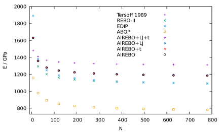
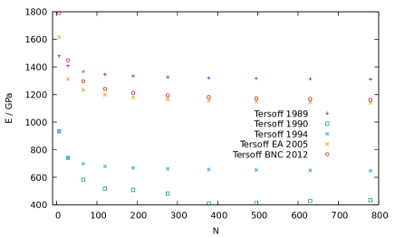
Figure 1: Young’s modulus of graphene for various sizes and potentials.

The experimental value for the Young’s modulus of graphene is about 1 TPa [24], which is also reproduced as 1.05 TPa by DFT calculations for this regular structure [25]. Figure 1 shows the results obtained with the various potentials on the l.h.s., whereas the r.h.s. displays the moduli obtained for several versions of the Tersoff potential. The modulus turns out to be isotropic in accordance with Refs. [26, 27]. The majority of potentials converges with $N$ against values for the modulus in the range of $1.1\dots 1.3$ TPa. The various investigated AIREBO potentials yield identical results. The EDIP potential comes closest to 1 TPa, practically on top with REBO-II, whereas the ABOP modulus falls below 0.8 TPa.

The chosen Tersoff potentials, displayed on the r.h.s. of Fig. 1, exhibit a similar spread of results. Earlier parameterizations of 1989 and 1994 deviate by about 0.3 TPa from the value of 1 TPa, whereas the more recent parameterizations of 2005 and 2012 yield values of 1.1 TPa similar to the EDIP or REBO-II potentials. It should be noted that the Tersoff potential of 1990 does not reproduce the correct graphene structure in our simulations.

For C-C- bond distances compare table 1.

3.2 Carbon Nanotubes

The investigated carbon nanotube (CNT) is a (20,20) tube with armchair geometry. In the investigation we varied the number of carbon atoms $N$, which is also a measure of length.

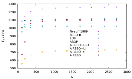
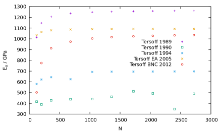
Figure 2: Young’s modulus of a (20,20) CNT with armchair geometry along the tube, taken as $x$-direction, for various sizes and potentials.

Since CNTs share the $sp^{2}$ structure with graphene, one would expect that Young’s moduli of single walled CNTs are very similar to that of graphene, which is indeed the case at least for large enough radii [28, 29]. For our calculations this similarity also holds. Again, the majority of potentials converges with $N$ against values in the range of now $1.0\dots 1.3$ TPa, see l.h.s. of Fig. 2. The various investigated AIREBO potentials once more yield identical results. The EDIP potential comes closest to 1 TPa, again together with REBO-II, whereas the modulus calculated with ABOP again stays below 0.8 TPa.

Also for the Tersoff potentials we obtain results similar to those for graphene, compare r.h.s. of Fig. 2. The large deviation for the Tersoff potentials of 1990 and 1994 correlates again with deficiencies to reproduce the structure. Using the version of 1994 the transverse section of the CNT is not a circle but more a rounded square in our simulations, whereas we could not obtain a reasonable structure with the 1990 version at all.

For C-C- bond distances compare table 1.

3.3 Diamond

The studied diamond structures had a size of about $\sqrt[3]{N}\times\sqrt[3]{N}\times\sqrt[3]{N}$. We performed simulations up to linear sizes of 20 atomic positions, which appears to be sufficient for the conclusions of this paper.

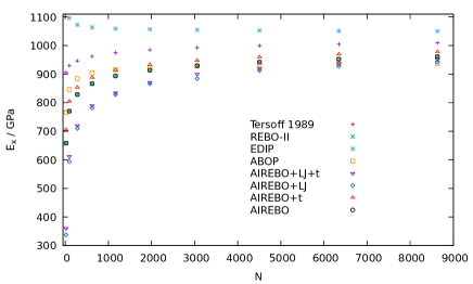
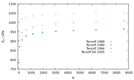
Figure 3: Young’s modulus of diamond taken along the $x$-direction shown in Fig. 4 for various sizes and potentials.

The experimental value of Young’s modulus was determined rather early in 1940 as $5.5\times 10^{12}$ dynes per sq. cm ($=0.55$ TPa) [30], which we would like to cite for curiosity. Since the modulus is direction-dependent, modern investigations yield an average of about $\overline{E}=1.15$ TPa [31] with values spreading between 1.05 TPa and 1.21 TPa [32]. In our simulations we find a rather good overall agreement between all potentials shown on the l.h.s. of Fig. 3. Although not yet fully converged to the thermodynamic limit for the largest calculated $N$, one clearly sees that all results agree with $(1\pm 0.07)$ TPa. REBO-II does not coincide with EDIP this time, but now with AIREBO without Lennard-Jones and torsion (AIREBO). Among the Tersoff potentials shown on the r.h.s. of Fig. 3 the 2005 parameterization yields a similarly good result, whereas the parameterizations of 1990 and 1994 again deviate towards too small values.

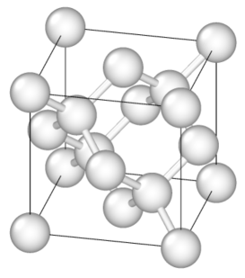
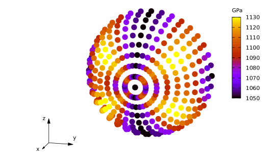
Figure 4: Structure – graphics produced with OVITO [33] – and directions as well as Young’s modulus of diamond taken in various directions of the northern hemisphere around the positive $x$-direction for $N=8631$ and the EDIP potential.

The directional variation of the modulus was investigated for the EDIP potential for the largest considered system size of $N=8631$. As can be seen in Fig. 4 the potential reproduces nicely the experimental variation of the modulus.

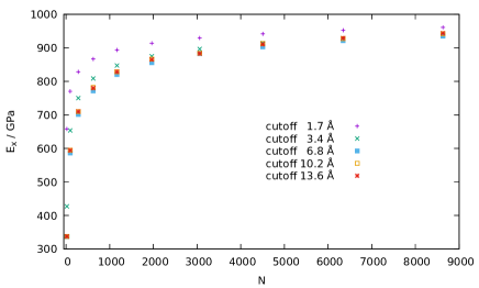
Figure 5: Young’s modulus of diamond taken along the $x$-direction shown in Fig. 4 for the AIREBO+LJ potential with various cutoffs.

Besides of the importance to describe the $sp^{3}$-bonding correctly, long-range interactions may play an important role in diamond. This question is investigated in Fig. 5, where the results derived from the AIREBO potential with additional long-range Lennard-Jones part, but without torsion, i.e. AIREBO+LJ, are displayed. The result is somewhat non-intuitive, no clear dependence on the range cutoff could be seen; all results are very close to each other with the exception of the smallest cutoff.

Table 1: Ground-state dimensions in Å of graphene, CNT, and diamond for the investigated potentials. (* No proper ground state structure found; $\dagger$ anisotropic.)

potential	graphene	CNT	diamond
	C-C distance	C-C distance	lattice const.
EDIP [12]	1.42	1.42	3.56
REBO-II [16]	1.42	1.42	3.58
ABOP [21]	1.42	1.424, 1.417 $\dagger$	3.46
Tersoff 89 [18]	1.46	1.46	3.57
Tersoff 90 [19]	*	*	3.56
Tersoff 94 [20]	1.55	*	3.56
Tersoff BNC [34, 35]	1.44	1.44	-
Tersoff EA [36]	1.48	1.48	3.57
AIREBO+LJ+t [22]	1.40	1.41	3.58
AIREBO+LJ [22]	1.40	1.40	3.58
AIREBO+t [22]	1.40	1.40	3.58
AIREBO [22]	1.40	1.40	3.58
experimental	1.42	1.42	3.567

As additional information about the performance of classical carbon potentials implemented in LAMMPS we provide ground-state C-C distances for graphene and the CNT as well as the lattice constant for diamond in table 1. As one can see, not all potentials perform equally well with respect to these characteristic distances. The EDIP potential meets all experimental numbers. Since the Tersoff-2012 potential was designed for B, C, and BN-C hybrid based graphene like nano structures, we did not use it for diamond.

4 Discussion and Outlook

For the investigated observable (Young’s modulus) and the chosen carbon materials it turns out that Marks’ improved EDIP potential and REBO-II [16] perform overall good with slight differences for diamond. REBO-II reacts somewhat softer to elongations for diamond which is very likely related to the smaller cutoff of the potential. EDIP uses a longer range of 3.2 Å, whereas REBO-II uses a cosine cutoff between 1.7 and 2.0 Å. This difference does not matter for graphene and CNTs. Both potentials lack long-range van der Waals components.

The potential ABOB [21] is consistently too soft for all three materials; for the $sp^{2}$ materials the deviation is as large as 20 %, for diamond the situation is better.

Among the class of Tersoff potentials the LAMMPS implementations of the parameterizations of 1990 [19] and 1994 [20] produce untrustworthy results. Even the relatively simple ground state structures of graphene and CNTs turned out to be wrong, compare also table 1. Reference [10] recommends the Tersoff potential for modeling of diamond. In view of our results this recommendation holds only for Tersoff 89 [18] and Tersoff EA [36].

For the observable studied in this paper we noticed that the variants of AIREBO do not differ significantly. We also noticed that although the LAMMPS documentation on AIREBO states that “If both of the LJ an torsional terms are turned off, it becomes the 2nd-generation REBO potential, with a small caveat on the spline fitting procedure mentioned below.”, our results for the CNT and graphene differ by more than what would be compatible “a small caveat”.

This article is published in full length in Beilstein J. Nanotechnol. 20??, ?, No. ?.