Three particle quantization condition in a finite volume:
2. general formalism and the analysis of data

Abstract

We derive the three-body quantization condition in a finite volume using an effective field theory in the particle-dimer picture. Moreover, we consider the extraction of physical observables from the lattice spectrum using the quantization condition. To illustrate the general framework, we calculate the volume-dependent three-particle spectrum in a simple model both below and above the three-particle threshold. The relation to existing approaches is discussed in detail.

I Introduction

The extraction of physical observables in sectors containing three and more particles remains one of the main challenges in lattice QCD. In contrast, this issue has already been settled in the one- and two-particle sectors. Namely, in the one-particle sector one determines the effective masses of stable particles. The infinite-volume limit is straightforward as lattice artifacts are exponentially suppressed at large volumes. In the case of the elastic two-body scattering, the celebrated Lüscher formula Luescher-torus algebraically relates the finite-volume energy eigenvalues to the infinite-volume scattering phase shift at the same energies. The approach remains conceptually the same for coupled-channel inelastic scattering Lage-KN ; Lage-scalar ; He ; Sharpe ; Briceno-multi ; Liu ; PengGuo-multi and has already been used to analyze the data in the two-channel system Wilson-pieta . A related approach that boils down to using a different parameterization of the infinite-volume amplitudes goes under the name of “unitary ChPT in a finite volume” oset ; Doring-scalar ; oset-in-a-finite-volume and has already been used in Ref. Bolton:2015psa to analyze $P$-wave $\pi\pi$ scattering and to study the properties of the $\rho$-meson. When the number of coupled channels is large, it might be advantageous to directly extract the real and imaginary parts of the optical potential in selected channels optical (note also the recent work Hansen:2017mnd , which aims at the extraction of the total width of the resonances decaying into the multiple channels). An alternative scheme aims at the extraction of hadronic potentials from the data HAL-essentials ; HAL-derivatives (see, e.g., Ref. HAL-multi for the generalization of this approach to the multi-channel case).

On the one hand, there is no such framework for intermediate states with three or more particles, although several attempts in this direction have been undertaken. The first formal investigation dates back to 2012, when it was rigorously shown that the three-body spectrum in a finite volume is determined solely by the three-body $S$-matrix elements in the infinite volume Polejaeva:2012ut . In the following years, further important aspects of the three-body problem in a finite volume have been addressed Meissner:2014dea ; Guo:2016fgl ; Guo:2017ism ; Briceno:2012rv ; Hansen:2014eka ; Hansen:2015zga ; Hansen:2015zta ; Hansen:2016fzj ; Hansen:2016ync ; Briceno:2017tce . In particular, the relativistic three-particle quantization condition in a finite volume has been obtained in Refs. Hansen:2014eka ; Hansen:2015zga ; Briceno:2017tce . In their subsequent papers, the authors were able to demonstrate that the framework is capable of reproducing known results, e.g., for the many-body ground-state energy or the energy shift of the three-body bound state in a finite volume. Despite this success, the quantization condition in these papers is not yet given in a form suitable for the analysis of the real lattice data: The whole formalism is still very complicated and the relation to the physical observables is not transparent. Finally, we mention Refs. Kreuzer:2010ti ; Kreuzer:2009jp ; Kreuzer:2008bi ; Kreuzer:2012sr , which addressed the three-body problem in a finite volume numerically using an effective field theory in the particle-dimer picture. Their numerical results for the finite volume spectrum strongly support the statement that the spectrum does not depend on the off-shell behavior of the three-body amplitudes, which was first proven in Ref. Polejaeva:2012ut and confirmed in Ref. Hansen:2014eka . These studies also suggest a strategy for analytical investigations of three-body dynamics in a finite volume.

On the other hand, recent years have seen a steady progress in lattice simulations involving three- and more-particle states. As a prominent example, we cite the numerous attempts to calculate the mass of the Roper resonance and solve the problem of the level ordering between this resonance and the $N^{*}(1535)$ Mathur:2003zf ; Guadagnoli:2004wm ; Leinweber:2004it ; Sasaki:2005ap ; Sasaki:2005ug ; Burch:2006cc ; Liu:2014jua ; Mahbub:2010jz ; Lasscock:2007ce ; Lang:2016hnn . It is a well known experimental fact that the Roper resonance decays with a significant probability (up to 40%) into the final state of a nucleon and two pions. Hence, a reliable extraction of its parameters is impossible without solving the three-body problem in a finite volume. Furthermore, a rapid advance of lattice nuclear simulations Beane:2010em ; Beane:2012vq ; Chang:2015qxa , as well as chiral effective field theories on the lattice Epelbaum:2009pd ; Epelbaum:2011md ; Rokash:2013xda ; Elhatisari:2015iga , provide us with data that can be properly analyzed, if and only if the few-body dynamics in a finite volume is understood. Otherwise, the extraction of reaction rates, elastic and inelastic cross sections, etc. from such calculations is not possible.

In our opinion, the main question which should be answered is the following: what is the optimum set of infinite-volume parameters (observables) of the three-body system which can be extracted directly from the data? To illustrate this question, we refer again to two-body elastic scattering. In this case, we have one measured lattice observable (the energy level) vs. one infinite-volume observable (the phase shift at the same energy). These two are unambiguously related via the Lüscher equation. In the two-channel case, we have again one finite volume energy level but three independent infinite-volume observables ($K$-matrix elements at the same energy). Thus, the most convenient strategy consists of parameterizing the energy-dependence of the multi-channel $K$-matrix in terms of a few parameters (resonance locations, residua, threshold expansion parameters) and fitting all available lattice data in a given energy interval with this parameterization (see, e.g., Wilson-pieta ). In the next step, having fixed these parameters, we may reliably determine the $K$-matrix elements everywhere in the given energy interval.

In case of three particles, much effort has been put into obtaining an analog of the Lüscher equation through collecting all infinite-volume contributions into the three-body $K$-matrix Polejaeva:2012ut ; Hansen:2014eka ; Hansen:2015zga ; Briceno:2017tce . The result is quite complicated and, in our opinion, is not well suited for the analysis of lattice data. For example, “smooth cutoffs” should be made and an “unconventional” $K$-matrix should be introduced at the intermediate stage. We argue in this paper that most of these complications stem from the inappropriate choice of parameters. Using the particle-dimer formalism, we arrive at a rather simple parameterization of the infinite-volume three-body $S$-matrix as well as the three-body spectrum in a finite volume. This provides a framework for the analysis of lattice data.

The layout of the paper is as follows. In Section II, we briefly review the infinite-volume framework for the description of the two- and three-body sectors, which is based on non-relativistic effective Lagrangians. The transition to the particle-dimer picture and the issue of the off-shell behavior is discussed in detail. In Section III, we consider the same theory in a finite volume and discuss the strategy for the lattice data analysis. A simple illustration is provided for the statement that the finite-volume spectrum is determined only by on-shell three-body $S$-matrix elements. In this section, we also present the results of the numerical calculations of the volume-dependent three-body spectrum, both below and above the three-particle threshold. In Section IV, we make a detailed comparison with the existing approaches. Finally, Section V contains our conclusions.

II Infinite volume

II.1 Two-particle sector

In order to simplify the formalism and highlight the central conceptual issues, we consider the interaction of three identical non-relativistic scalars. In addition, we assume that two-to-three particle transitions are forbidden. Thus for applications to QCD, our final result still needs to be decorated with spin indices, relativistic boosts into non-rest frames, etc. These effects can be included in a second stage. For example, the coupling of the two- and three-particle sectors can be included along the lines of Ref. Briceno:2017tce . We stress that none of these issues affect the essence of the problem considered in this paper.

The three-particle Lagrangian can be written in the following form

$${\cal L}=\psi^{\dagger}\biggl{(}i\partial_{0}+\frac{\nabla^{2}}{2m}\biggr{)}\psi+{\cal L}_{2}+{\cal L}_{3}\,,$$ (1)

where $\psi(x)$ denotes a non-relativistic field with the propagator

$$i\langle 0|T\psi(x)\psi^{\dagger}(y)|0\rangle=\int\frac{d^{4}p}{(2\pi)^{4}}\,\frac{e^{-ip(x-y)}}{w({\bf p})-p_{0}-i0}\,,\quad\quad w({\bf p})=\frac{{\bf p}^{2}}{2m}\,,$$ (2)

$m$ is the mass of the particle, and ${\cal L}_{2},{\cal L}_{3}$ denote the two- and three-particle interaction terms, respectively.

Let us start from the two-particle term. It contains a tower of operators of increasing mass dimension or, equivalently, an increasing number of space derivatives

$${\cal L}_{2}=-\frac{C_{0}}{2}\,\psi^{\dagger}\psi^{\dagger}\psi\psi+\frac{C_{2}}{4}\,(\psi^{\dagger}\tensor{\nabla}^{2}\psi^{\dagger}\psi\psi+\mbox{h.c.})+O(\nabla^{4})\,.$$ (3)

Here, the first term corresponds to a non-derivative interaction which is purely S-wave. In the second term, we employ the Galilean invariant derivative operator $\tensor{\nabla}\equiv(\roarrow{\nabla}-\loarrow{\nabla})/2$, which is understood to act only on the fields immediately left and right of the operator. For identical spinless particles there are no odd partial waves, so the contribution of higher partial waves starts at $O(\nabla^{4})$.

It is more convenient to use the momentum representation for the analysis of the higher-order terms. Because of Galilei invariance, the interaction does not depend on the center-of-mass momentum. It is characterized by the relative momenta of the two particles in the final and initial states, ${\bf p}$ and ${\bf q}$, respectively. Using rotational invariance and Bose-symmetry, the matrix element of the interaction Lagrangian between the two-particle states can be written in the form

$$\langle{\bf P},{\bf p}|{\cal L}_{2}|{\bf q},{\bf P}\rangle=\sum_{n,m,k=0}^{\infty}l_{nmk}{\bf p}^{2n}{\bf q}^{2m}({\bf p}{\bf q})^{2k}\,,$$ (4)

where $l_{nmk}$ are linear combinations of $C_{0},C_{2},\ldots$.

Furthermore, the expression $q_{i_{1}}\cdots q_{i_{2k}}$ is given by a sum of a traceless tensors of rank $2k$ and less, and terms containing the Kronecker symbol. For example,

$$q_{i}q_{j}=\biggl{(}q_{i}q_{j}-\frac{1}{3}\,\delta_{ij}{\bf q}^{2}\biggr{)}+\frac{1}{3}\,\delta_{ij}{\bf q}^{2}\,,$$ (5)

and similar expressions hold for higher order tensors. The first term in brackets is traceless and corresponds to a D-wave. The Kronecker symbol $\delta_{ij}$ in the second term will be convoluted with $p_{i}p_{j}$ and yields ${\bf p}^{2}$, corresponding to a S-wave. Continuing this way, we obtain

$$\langle{\bf P},{\bf p}|{\cal L}_{2}|{\bf q},{\bf P}\rangle=\sum_{n,m,k=0}^{\infty}l^{\prime}_{nmk}{\bf p}^{2n}{\bf q}^{2m}\sum_{i_{1},\cdots i_{2k}}F_{i_{1},\cdots i_{2k}}({\bf p})F_{i_{1},\cdots i_{2k}}({\bf q})\,,$$ (6)

where the $F_{i_{1},\cdots i_{2k}}$ are traceless tensors in all indices and correspond to even orbital momentum $L=2k$, whereas $l^{\prime}_{nmk}$ are linear combinations of $l_{nmk}$. Hence, we obtain a clear-cut classification of the operators of the Lagrangian in the partial waves and – within a sector with a given value of the orbital momentum – in powers of momenta ${\bf p}^{2n}{\bf q}^{2m}$.

Next, we consider the matching of the couplings $C_{0},C_{2},\ldots$ to the physical observables. We limit ourselves to a sector with a fixed value of the orbital momentum (say, the S-wave). The available observables for fitting are the effective-range parameters

$$p\cot\delta(p)=-\frac{1}{a}+\frac{r_{e}}{2}\,p^{2}+\sum_{n=2}^{\infty}b_{2n}p^{2n}\,,\quad\quad p^{2}={\bf p}^{2}\,.$$ (7)

At order ${\bf p}^{4}$ we have two independent operators

$${\cal L}_{2}^{S-wave} = -\frac{C_{0}}{2}\,\psi^{\dagger}\psi^{\dagger}\psi\psi+\frac{C_{2}}{4}\,(\psi^{\dagger}\tensor{\nabla}^{2}\psi^{\dagger}\psi\psi+\mbox{h.c.})$$

$$- \frac{C_{4}}{4}\,(\psi^{\dagger}\tensor{\nabla}^{4}\psi^{\dagger}\psi\psi+\psi^{\dagger}\tensor{\nabla}^{2}\psi^{\dagger}\psi\tensor{\nabla}^{2}\psi+\mbox{h.c.})$$

$$- \frac{C_{4}^{\prime}}{4}\,(\psi^{\dagger}\tensor{\nabla}^{4}\psi^{\dagger}\psi\psi-\psi^{\dagger}\tensor{\nabla}^{2}\psi^{\dagger}\psi\tensor{\nabla}^{2}\psi+\mbox{h.c.})+O(\nabla^{6})\,,$$

$$\langle{\bf P},{\bf p}|{\cal L}_{2}^{S-wave}|{\bf q},{\bf P}\rangle = -2C_{0}-C_{2}({\bf p}^{2}+{\bf q}^{2})-C_{4}({\bf p}^{2}+{\bf q}^{2})^{2}-C_{4}^{\prime}({\bf p}^{2}-{\bf q}^{2})^{2}\,.$$ (8)

It is clear that the matching to $b_{4}$ from Eq. (7) determines the constant $C_{4}$, whereas the term with $C_{4}^{\prime}$ vanishes on the energy shell ${\bf p}^{2}={\bf q}^{2}$ and thus is not fixed from matching. Moreover, using the equations of motion

$$\biggl{(}i\partial_{0}+\frac{\nabla^{2}}{2m}\biggr{)}\psi=C_{0}\psi^{\dagger}\psi\psi+\cdots\,,$$ (9)

we find that the off-shell term is proportional to a total time derivative (modulo surface terms)

$$\psi^{\dagger}\tensor{\nabla}^{4}\psi^{\dagger}\psi\psi-\psi^{\dagger}\tensor{\nabla}^{2}\psi^{\dagger}\psi\tensor{\nabla}^{2}\psi+\mbox{h.c.}\propto\partial_{0}^{2}(\psi^{\dagger}\psi^{\dagger}\psi\psi)\,,$$ (10)

and, hence, does not affect the equations of motion. Note that the above relation holds up to terms containing six fields. Consequently, if the three-particle sector is also considered, the off-shell terms in the two-particle sector can be eliminated in favor of the three-particle forces.

Another statement concerns the two-particle spectrum in a finite volume. The validity of the Lüscher equation implies that such off-shell terms do not affect the spectrum, which is solely determined by the on-shell $S$-matrix elements. Physically, this stems from the existence of two widely separated scales – the box size $L$ and the typical interaction range $R$, with $R\ll L$. This means that the two-particle wave function near the boundaries is given by its asymptotic form determined by the phase shift. Hence, only this quantity enters the finite-volume quantization condition. Our aim is to verify the same statement in the three-particle sector as well, where it looks less intuitive. Namely, there exist regions in the configuration space, where two out of three-particles are close to each other and the third particle is far away (at the distances of order of the box size $L$). Nevertheless, as we shall see, the statement still holds.

Figure 1: $T$-matrix in the non-relativistic theory. The filled boxes represent the tree-level Lagrangian containing the low-energy couplings $C_{0},C_{2},C_{4},\ldots$.

The two-body scattering $T$-matrix is given by the sum of the bubble diagrams shown in Fig. 1. On the mass shell, is is equal to

$$T=\frac{8\pi/m}{p\cot\delta(p)-ip}\,,$$ (11)

where $p\cot\delta(p)$ is given by the effective-range expansion (7).

II.2 Dimer formalism

Next, we consider the introduction of the dimer field in the context of the pure two-body problem. Note first that it is allowed to rewrite the above expression in a form

$$\langle{\bf P},{\bf q}|{\cal L}_{2}|{\bf p},{\bf P}\rangle=\sigma\sum_{k=0}^{\infty}f({\bf p}^{2})f({\bf q}^{2})\sum_{i_{1},\cdots i_{2k}}F_{i_{1},\cdots i_{2k}}({\bf p})F_{i_{1},\cdots i_{2k}}({\bf q})\,,$$ (12)

where $f({\bf p}^{2})=f_{0}+f_{1}{\bf p}^{2}+\ldots$. Further, $\sigma=-1$ if $C_{0}>0$ and vice versa. Since, at a given order in ${\bf p}^{2}$, there is only one physically relevant constant that can be matched on shell, one may recursively express the couplings $f_{0},f_{1},\ldots$ through the effective range parameters.

Now, let $T_{i_{1},\cdots i_{2k}}$ be a field completely traceless in its indices, which describes a dimer with spin equal to $2k$. One may write down the Lagrangian

$${\cal L} = \psi^{\dagger}\biggl{(}i\partial_{0}+\frac{\nabla^{2}}{2m}\biggr{)}\psi+\sigma\sum_{k=0}^{\infty}\sum_{i_{1},\cdots i_{2k}}T_{i_{1},\cdots i_{2k}}^{\dagger}T_{i_{1},\cdots i_{2k}}$$ (13)

$$+ \biggl{(}\sum_{k=0}^{\infty}\sum_{i_{1},\cdots i_{2k}}T_{i_{1},\cdots i_{2k}}^{\dagger}\psi\bigl{[}f(-i\nabla)F_{i_{1},\cdots i_{2k}}(-i\nabla)\bigr{]}\psi+\mbox{h.c.}\biggr{)}\,,$$

where $\psi\bigl{[}f(-i\nabla)F_{i_{1},\cdots i_{2k}}(-i\nabla)\bigr{]}\psi$ is a shorthand notation (the operator $\nabla$ in the second line should be interpreted as a “Galilei-invariant” operator, see the discussion below Eq. (3)). To explain this notation, consider first the spinless dimer $k=0$. Writing down $f(-i\nabla)=f_{0}+f_{1}(-i\nabla)^{2}+\ldots$, and taking into account the Bose-symmetry factors, we get

$$\psi\bigl{[}f_{0}\bigr{]}\psi = \frac{1}{2}\,f_{0}\psi\psi\,,$$

$$\psi\bigl{[}f_{1}(-i\nabla)^{2}\bigr{]}\psi = -\frac{1}{4}\,f_{1}(\psi\nabla^{2}\psi-\nabla_{i}\psi\nabla_{i}\psi)\,,$$ (14)

and so on. For the spin-2 dimer (i.e., $k=1$ we have)

$$\psi\bigl{[}F_{ij}(-i\nabla)\bigr{]}\psi = \psi\biggl{[}\frac{3}{2}(-i\nabla)_{i}(-i\nabla)_{j}-\frac{1}{2}\,\delta_{ij}(-i\nabla)^{2}\biggr{]}\psi$$ (15)

$$= -\frac{3}{8}\,\psi\nabla_{i}\nabla_{j}\psi+\frac{3}{8}\,\nabla_{i}\psi\nabla_{j}\psi+\frac{1}{8}\,\delta_{ij}\psi\nabla^{2}\psi-\frac{1}{8}\,\delta_{ij}\nabla_{k}\psi\nabla_{k}\psi\,,$$

and so on. In the CM frame, one may perform the partial integration, leading to the same result as before.

The dimer field $T_{i_{1},\cdots i_{2k}}$ is an auxiliary field. Integrating it out with the use of the equations of motion, or using the path integral, it is straightforward to verify that the dimer formalism on the energy shell is mathematically equivalent to the theory defined by the two-body Lagrangian, Eq. (II.1). In particular, the on-shell $T$-matrix is again given by Eq. (11), also in non-rest frames. Putting it differently, the dimer picture is not an approximation – it is an alternative description of two-body scattering. The scattering in higher partial waves is represented through dimers with arbitrary integer spins.

II.3 Three-particle sector

Next, let us turn to the three-particle sector and write down the Lagrangian. At leading order, it is given by

$${\cal L}_{3}^{LO}=-\frac{D_{0}}{6}\,\psi^{\dagger}\psi^{\dagger}\psi^{\dagger}\psi\psi\psi\,.$$ (16)

Further, we turn to the next-to-leading order. As in the two-particle sector, it is easier to carry out the classification of the derivative terms in momentum space. To keep the discussion transparent, we restrict ourselves to the center-of-mass frame ${\bf p}_{1}+{\bf p}_{2}+{\bf p}_{3}={\bf q}_{1}+{\bf q}_{2}+{\bf q}_{3}={\bf 0}$ in the three-particle sector. It is always possible to rewrite the expressions in a manifestly Galilei-invariant form using Galilei invariant derivatives. At next-to-leading order, we have the following invariants:

$${\bf p}_{i}^{2}\,,~{}{\bf p}_{i}{\bf p}_{j}\,,~{}{\bf q}_{i}^{2}\,,~{}{\bf q}_{i}{\bf q}_{j}\,,~{}{\bf p}_{i}{\bf q}_{i}\,,~{}{\bf p}_{i}{\bf q}_{j}\,,\quad\quad i\neq j\,,\quad i,j=1,2,3\,.$$ (17)

Bose-symmetry, time invariance and Hermiticity exclude all structures but one

$$\langle{\bf q}|{\cal L}_{3}^{NLO}|{\bf p}\rangle=D_{2}\sum_{i=1}^{3}({\bf p}_{i}^{2}+{\bf q}_{i}^{2})$$ (18)

which in position space gives

$${\cal L}_{3}^{NLO}=-\frac{D_{2}}{12}\,(\psi^{\dagger}\psi^{\dagger}\nabla^{2}\psi^{\dagger}\,\psi\psi\psi+\mbox{h.c.})\,.$$ (19)

Let us now consider next-to-next-to-leading order. Using the condition ${\bf p}_{1}+{\bf p}_{2}+{\bf p}_{3}={\bf q}_{1}+{\bf q}_{2}+{\bf q}_{3}={\bf 0}$ and taking into account the Hermiticity of the Lagrangian and Bose-symmetry, the set of linearly independent invariants is

$$O = ({\bf p}_{1}^{4}+{\bf p}_{2}^{4}+{\bf p}_{3}^{4})+({\bf q}_{1}^{4}+{\bf q}_{2}^{4}+{\bf q}_{3}^{4})\,,$$

$$O^{\prime} = \bigl{[}({\bf p}_{1}^{2}+{\bf p}_{2}^{2}+{\bf p}_{3}^{2})+({\bf q}_{1}^{2}+{\bf q}_{2}^{2}+{\bf q}_{3}^{2})\bigr{]}^{2}\,,$$

$$O^{\prime\prime} = \bigl{[}({\bf p}_{1}^{2}+{\bf p}_{2}^{2}+{\bf p}_{3}^{2})-({\bf q}_{1}^{2}+{\bf q}_{2}^{2}+{\bf q}_{3}^{2})\bigr{]}^{2}\,.$$ (20)

Note that we have written down only the terms that contribute to the S-wave. There are also D-wave contributions generated at this order, say, by terms of the type $\sum\limits_{i,j=1}^{3}({\bf p}_{i}{\bf q}_{j})^{2}$. For illustrative purposes, however, we restrict ourselves to the S-wave contribution only.

In position space, we get

$${\cal L}_{3}^{NNLO} = \frac{D_{4}}{12}\,\bigl{(}\psi^{\dagger}\psi^{\dagger}\nabla^{4}\psi^{\dagger}\,\psi\psi\psi+\mbox{h.c.}\bigr{)}$$ (21)

$$+ \frac{D_{4}^{\prime}}{12}\,\bigl{(}(\psi^{\dagger}\psi^{\dagger}\nabla^{4}\psi^{\dagger}\,\psi\psi\psi+2\psi^{\dagger}\nabla^{2}\psi^{\dagger}\nabla^{2}\psi^{\dagger}\,\psi\psi\psi+\mbox{h.c.})+6\psi^{\dagger}\psi^{\dagger}\nabla^{2}\psi^{\dagger}\,\psi\psi\nabla^{2}\psi\bigr{)}$$

$$+ \frac{D_{4}^{\prime\prime}}{12}\,\bigl{(}(\psi^{\dagger}\psi^{\dagger}\nabla^{4}\psi^{\dagger}\,\psi\psi\psi+2\psi^{\dagger}\nabla^{2}\psi^{\dagger}\nabla^{2}\psi^{\dagger}\,\psi\psi\psi+\mbox{h.c.})-6\psi^{\dagger}\psi^{\dagger}\nabla^{2}\psi^{\dagger}\,\psi\psi\nabla^{2}\psi\bigr{)}$$

The low-energy coupling $D_{4}^{\prime\prime}$ is analogous to the “off-shell” coupling $C_{4}^{\prime}$ considered in the two-particle sector – at tree level, it does not contribute to the three-particle amplitude.

Furthermore, using the equations of motion it can be shown that

$$-(2m)^{2}\partial_{0}^{2}(\psi^{\dagger}\psi^{\dagger}\psi^{\dagger}) = 6\psi^{\dagger}\nabla^{2}\psi^{\dagger}\nabla^{2}\psi^{\dagger}+3\psi^{\dagger}\psi^{\dagger}\nabla^{4}\psi^{\dagger}+\cdots\,$$

$$-(2m)^{2}\partial_{0}^{2}(\psi\psi\psi) = 6\psi\nabla^{2}\psi\nabla^{2}\psi+3\psi\psi\nabla^{4}\psi+\cdots\,,$$

$$-(2m)^{2}\partial_{0}(\psi^{\dagger}\psi^{\dagger}\psi^{\dagger})\partial_{0}(\psi\psi\psi) = -9\psi^{\dagger}\psi^{\dagger}\nabla^{2}\psi^{\dagger}\psi\psi\nabla^{2}\psi+\cdots\,,$$ (22)

where the ellipses stand for terms containing more field operators. Taking these equations into account, it is straightforward to see that the term proportional to $D_{4}^{\prime\prime}$ is a total time derivative

$$-\frac{D_{4}^{\prime\prime}}{36}\,(2m)^{2}\partial_{0}^{2}(\psi^{\dagger}\psi^{\dagger}\psi^{\dagger}\psi\psi\psi)\,,$$ (23)

and therefore does not contribute to the equations of motion.

II.4 Insertion of the off-shell terms into Feynman diagrams

As we have seen, the on-shell three-body scattering $T$-matrix does not depend on the low-energy coupling $D_{4}^{\prime\prime}$. We now want to expand this argument beyond tree level and show that the $T$-matrix does not depend on $D_{4}^{\prime\prime}$ at all. This would have been easy in the two-body sector: one would use dimensional regularization and argue that the off-shell terms in perturbation theory lead to no-scale integrals that vanish in this regularization. The final answer then should not depend on the regularization used. This argument, however, rests on the fact that the two-body potential is a low-energy polynomial. This is not true anymore in the three-body sector, where the pair interactions give rise to a non-polynomial potential. For this reason, we have to examine the perturbation series in the three-body sector more carefully.

The three-body $T$-matrix obeys the Lippmann-Schwinger equation

$$T=V+VG_{0}T\,,$$ (24)

where $G_{0}$ is the free three-body Green function, and $V$ denotes the kernel (potential) of this equation – the sum of all Feynman diagrams which can not be made disconnected by cutting exactly three particle lines. Of course, it is well known that the above equation is mathematically ill-defined. All two-body interactions should be summed up first, leading to the Faddeev equations. This fact, however, will not bother us in the following, since we consider the Lippmann-Schwinger equation merely as a tool to generate a full set of Feynman diagrams in the three-body $T$-matrix.

According to the discussion in the previous subsection, we may split off the off-shell part from the potential $V$:

$$V=\bar{V}+V^{\prime}\,,$$ (25)

where, in our case, $V^{\prime}=\kappa(E_{f}-E_{i})^{2},~{}\kappa\propto D_{4}^{\prime\prime}$. Here, $E_{i}=\frac{1}{2m}\,({\bf q}_{1}^{2}+{\bf q}_{2}^{2}+{\bf q}_{3}^{2})$ and $E_{f}=\frac{1}{2m}\,({\bf p}_{1}^{2}+{\bf p}_{2}^{2}+{\bf p}_{3}^{2})$ are the initial and final three-particle energies, respectively. Further, it can be straightforwardly shown that

$$T=T^{\prime}+(1+T^{\prime}G_{0})\nu(1+G_{0}T^{\prime})\,,$$ (26)

where $T^{\prime}$ is the scattering matrix of the “off-shell” potential $V^{\prime}$ only:

$$T^{\prime}=V^{\prime}+V^{\prime}G_{0}T^{\prime}$$ (27)

and $\nu$ obeys the following equation

$$\nu=\bar{V}+\bar{V}(G_{0}+G_{0}T^{\prime}G_{0})\nu=\bar{\nu}+\bar{\nu}(G_{0}T^{\prime}G_{0})\nu\,,$$ (28)

where $\bar{\nu}$ is the scattering matrix on the potential $\bar{V}$ (without the “off-shell” term):

$$\bar{\nu}=\bar{V}+\bar{V}G_{0}\bar{\nu}\,.$$ (29)

Our aim is to demonstrate that

$$T\biggr{|}_{\mbox{on shell}}=\bar{\nu}\biggr{|}_{\mbox{on shell}}\,.$$ (30)

This aim can be achieved in a few consecutive steps. First of all, it is immediately seen that $T^{\prime}$ vanishes on shell. Indeed, using dimensional regularization, we get

$$T^{\prime}(E)=\kappa(E_{f}-E_{i})^{2}+\kappa^{2}(E_{f}-E)^{2}g_{0}(E)(E-E_{i})^{2}\,.$$ (31)

Here, $E$ is the off-shell energy (in general, $E\neq E_{i}\neq E_{f}$), and

$$g_{0}(E)=\int_{\bf k}\frac{1}{E({\bf k})-E-i0}\,,$$ (32)

where

$$\int_{\bf k}\doteq\int\frac{d^{d}{\bf k}_{1}}{(2\pi)^{3}}\,\frac{d^{d}{\bf k}_{2}}{(2\pi)^{3}}\,\frac{d^{d}{\bf k}_{3}}{(2\pi)^{3}}\,(2\pi)^{d}\delta^{d}({\bf k}_{1}+{\bf k}_{2}+{\bf k}_{3})\,,\quad\quad E({\bf k})=\frac{1}{2m}\,({\bf k}_{1}^{2}+{\bf k}_{2}^{2}+{\bf k}_{3}^{2})\,.$$ (33)

The expression (31) vanishes at $E_{i}=E_{f}=E$.

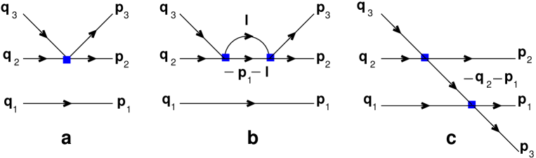
Figure 2: Lowest-order Feynman graphs emerging in the expansion of the quantity $\nu$.

Further, let us consider the quantity $T^{\prime}G_{0}\nu$ on shell:

$$T^{\prime}G_{0}\nu=\int_{\bf k}(\kappa(E_{f}-E_{\bf k})^{2}+\kappa^{2}(E_{f}-E)^{2}g_{0}(E)(E-E_{\bf k})^{2})\frac{1}{E_{\bf k}-E-i0}\,\nu\,.$$ (34)

The second term vanishes at $E_{f}=E$, while the first term can on the energy shell be rewritten as

$$T^{\prime}G_{0}\nu\biggr{|}_{\mbox{on shell}}=\kappa\int_{\bf k}(E-E_{\bf k})\nu\,.$$ (35)

This expression also vanishes, if $\nu$ is a low-energy polynomial. However, in general it is not. For this reason, let us consider a few typical diagrams shown in Fig. 2, in order to ensure that the above expression still leads to no-scale integrals. Let us start from the diagram shown in Fig. 2a which yields $\nu=2C_{0}(2\pi)^{d}\delta^{d}({\bf k_{1}}-{\bf p}_{1})$. Substituting this expression into into Eq. (35), we get

$$T^{\prime}G_{0}\nu\biggr{|}_{\mbox{on shell}}=2C_{0}\kappa\int\frac{d^{d}{\bf k}_{2}}{(2\pi)^{d}}\,\biggl{(}E-\frac{1}{2m}\bigl{(}{\bf p}_{1}^{2}+{\bf k}_{2}^{2}+({\bf k}_{2}+{\bf p}_{1})^{2}\bigr{)}\biggr{)}=0\,.$$ (36)

Next, let us consider the one-loop diagram shown in Fig. 2b. Carrying out the same steps as above, one obtains

$$T^{\prime}G_{0}\nu\biggr{|}_{\mbox{on shell}} = 4C_{0}^{2}\kappa\int\frac{d^{d}{\bf k}_{2}}{(2\pi)^{d}}\,\frac{d^{d}{\bf l}}{(2\pi)^{d}}\,\biggl{(}E-\frac{1}{2m}\bigl{(}{\bf p}_{1}^{2}+{\bf k}_{2}^{2}+({\bf k}_{2}+{\bf p}_{1})^{2}\bigr{)}\biggr{)}$$ (37)

$$\times \frac{2m}{{\bf p}_{1}^{2}+{\bf l}^{2}+({\bf p}_{1}+{\bf l})^{2}-2mE-i0}=0\,.$$

The last equality stems from the fact that the integral over ${\bf k}_{2}$ is a no-scale integral, even if $\nu$ is not a low-energy polynomial.

Finally, we consider the diagram shown in Fig. 2c. The result is given by

$$T^{\prime}G_{0}\nu\biggr{|}_{\mbox{on shell}} = 4C_{0}^{2}\kappa\int\frac{d^{d}{\bf k}_{1}}{(2\pi)^{d}}\,\frac{d^{d}{\bf k}_{2}}{(2\pi)^{d}}\,\biggl{(}E-\frac{1}{2m}\bigl{(}{\bf k}_{1}^{2}+{\bf k}_{2}^{2}+({\bf k}_{1}+{\bf k}_{2})^{2}\bigr{)}\biggr{)}$$ (38)

$$\times \frac{2m}{{\bf p}_{2}^{2}+{\bf k}_{1}^{2}+({\bf p}_{2}+{\bf k}_{1})^{2}-2mE-i0}=0\,.$$

This integral also vanishes because it is a no-scale integral with respect to the momentum ${\bf k}_{2}$.

This exhausts the list of the possible alternatives. Consequently, in general $T^{\prime}G_{0}\nu$ vanishes on shell, even if $\nu$ is not a low-energy polynomial. By the same token, $\nu G_{0}T^{\prime}$ and $T^{\prime}G_{0}\nu G_{0}T^{\prime}$ vanish on shell as well, leading to the conclusion that $T$ and $\nu$ coincide on the energy shell.

Finally, we focus of Eq. (28), which relates the quantities $\nu$ and $\bar{\nu}$. Consider the second iteration of this equation, $\bar{\nu}G_{0}T^{\prime}G_{0}\bar{\nu}$, where $T^{\prime}$ is given by Eq. (31). It is immediately seen that the contribution from the second term in Eq. (31) factorizes and vanishes on the energy shell, leading to an integral similar to the one given in Eq. (35). Using the simple algebraic identity

$$\frac{(E_{f}-E_{i})^{2}}{(E_{f}-E)(E_{i}-E)}=\frac{E_{f}-E_{i}}{E_{i}-E}-\frac{E_{f}-E_{i}}{E_{f}-E}\,,$$ (39)

the contribution from the first term can be also reduced to the integrals of the same type. Higher order terms can be considered in a similar way. Thus, on shell $\nu=\bar{\nu}$ and, consequently, Eq. (30) holds.

To summarize this rather lengthy but straightforward discussion, note that $\bar{\nu}$, defined by Eq. (29) is the three-body scattering $T$-matrix for $D_{4}^{\prime\prime}=0$. Thus, we have shown that the coupling constant $D_{4}^{\prime\prime}$ does not appear in the on-shell $T$ matrix (neither at tree level, nor as an insertion in higher-order Feynman diagrams) and can not be fixed from experimental input. We remind the reader that this coupling multiplies an operator that can be reduced to a total time derivative by using the equation of motion. In the infinite volume, the omission of such operators can not lead to observable consequences.

II.5 The dimer formalism in the three-particle sector

In this subsection, we write down the particle-dimer interaction Lagrangian, which is equivalent to the original three-particle Lagrangian. For simplicity, we restrict ourselves to the case of a scalar dimer. The generalization to the higher partial waves is straightforward.

We start from the Lagrangian (cf. Eq. (13) ),

$${\cal L} = \psi^{\dagger}\biggl{(}i\partial_{0}+\frac{\nabla^{2}}{2m}\biggr{)}\psi+\sigma T^{\dagger}T+\biggl{(}T^{\dagger}\psi\bigl{[}f(-i\nabla)\bigr{]}\psi+\mbox{h.c.}\biggr{)}$$ (40)

$$+ h_{0}T^{\dagger}T\psi^{\dagger}\psi+h_{2}T^{\dagger}T(\psi^{\dagger}\nabla^{2}\psi+\nabla^{2}\psi^{\dagger}\psi)$$

$$+ h_{4}T^{\dagger}T(\psi^{\dagger}\nabla^{4}\psi+\nabla^{4}\psi^{\dagger}\psi)+h_{4}^{\prime}T^{\dagger}T\nabla^{2}\psi^{\dagger}\nabla^{2}\psi+\cdots\,,$$

where

$$\psi\bigl{[}f(-i\nabla)\bigr{]}\psi = \frac{1}{2}\,\biggl{(}f_{0}\psi\psi+f_{1}\psi(-i\stackrel{{\scriptstyle\leftrightarrow}}{{\nabla}})^{2}\psi+f_{2}\psi(-i\stackrel{{\scriptstyle\leftrightarrow}}{{\nabla}})^{4}\psi+\cdots\biggr{)}\,,$$

$$\psi(-i\stackrel{{\scriptstyle\leftrightarrow}}{{\nabla}})^{2}\psi = \frac{1}{2}\,\biggl{(}-\psi\nabla^{2}\psi+\nabla_{i}\psi\nabla_{i}\psi\biggr{)}\,,\quad\mbox{and so on.}$$ (41)

Integrating out the dimer field, this Lagrangian can be rewritten as

$${\cal L} = \psi^{\dagger}\biggl{(}i\partial_{0}+\frac{\nabla^{2}}{2m}\biggr{)}\psi$$ (42)

$$- \frac{(\psi\bigl{[}f(-i\nabla)\bigr{]}\psi)^{\dagger}(\psi\bigl{[}f(-i\nabla)\bigr{]}\psi)}{\sigma+h_{0}\psi^{\dagger}\psi+h_{2}(\psi^{\dagger}\nabla^{2}\psi+\nabla^{2}\psi^{\dagger}\psi)+h_{4}(\psi^{\dagger}\nabla^{4}\psi+\nabla^{4}\psi^{\dagger}\psi)+h_{4}^{\prime}\nabla^{2}\psi^{\dagger}\nabla^{2}\psi}+\cdots\,.$$

Expanding the denominator, one gets the previous result in the two-particle sector. In the three-particle sector, the following operators emerge:

$${\cal L}_{3}=\frac{f_{0}^{2}h_{0}}{4}\,\psi^{\dagger}\psi^{\dagger}\psi^{\dagger}\psi\psi\psi+\biggl{(}-\frac{3f_{0}f_{1}h_{0}}{16}+\frac{f_{0}^{2}h_{2}}{4}\biggr{)}(\psi^{\dagger}\psi^{\dagger}\nabla^{2}\psi^{\dagger}\psi\psi\psi+\mbox{h.c.})+O(\nabla^{4})\,.$$ (43)

Here, we have used the fact that in the three-particle CM frame,

$$(\psi^{\dagger}\nabla^{2}\psi^{\dagger}-\nabla_{i}\psi^{\dagger}\nabla_{i}\psi^{\dagger})\psi^{\dagger}\psi\psi\psi=\biggl{(}\psi^{\dagger}\psi^{\dagger}\nabla^{2}\psi^{\dagger}-\frac{1}{2}\,\nabla_{i}(\psi^{\dagger}\psi^{\dagger})\nabla_{i}\psi^{\dagger}\biggr{)}\psi\psi\psi=\frac{3}{2}\,\psi^{\dagger}\psi^{\dagger}\nabla^{2}\psi^{\dagger}\psi\psi\psi\,.$$

Consequently,

• At order $\nabla^{0}$, the coupling constant $D_{0}$ is matched to $h_{0}$.

• At order $\nabla^{2}$, the coupling constant $D_{2}$ is matched to $h_{2}$.

• At order $\nabla^{4}$ we have three coupling constants $D_{4},D_{4}^{\prime},D_{4}^{\prime\prime}$ in the three-body formalism, to be matched to the two constants $h_{4},h_{4}^{\prime}$ in the particle-dimer formalism. This shows once more that one of the couplings ($D_{4}^{\prime\prime}$) is redundant and can be eliminated from the theory without changing the physical content.

Note also that the off-shell terms in particle-dimer scattering are essential and should not be eliminated. This is because the dimer does not have a fixed mass. The on-shell three-particle $T$-matrix can uniquely be related to the off-shell particle-dimer $T$-matrix.

II.6 The scattering equation

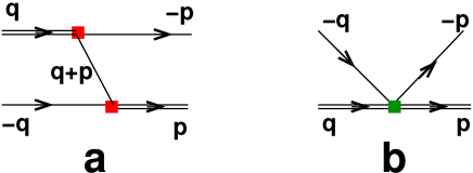
Figure 3: The kernel of the three-particle Lippmann-Schwinger equation: a) the exchange diagram between the particle and the dimer; b) local particle-dimer interactions with couplings $h_{0},h_{2},\ldots$.

In the simplest case, when only non-derivative interactions are present in the Lagrangian, the particle-dimer scattering equation takes the form (see Fig. 3)

$${\cal M}({\bf p},{\bf q};E)=Z({\bf p},{\bf q};E)+8\pi\int^{\Lambda}\frac{d^{3}{\bf k}}{(2\pi)^{3}}\,Z({\bf p},{\bf k};E)\tau({\bf k};E){\cal M}({\bf k},{\bf q};E)\,.$$ (45)

Here, $E$ denotes the total CM energy of three particles, $a$ denotes the S-wave scattering length, and

$$Z({\bf p},{\bf q};E) = \frac{1}{-mE+{\bf p}^{2}+{\bf q}^{2}+{\bf p}{\bf q}}+\frac{h_{0}}{mf_{0}^{2}}\,,$$

$$\tau({\bf k};E) = \frac{1}{-a^{-1}+\sqrt{\frac{3}{4}\,{\bf k}^{2}-mE}}\,.$$ (46)

The solution of the above equation unique because of the presence of the ultraviolet cutoff $\Lambda$. Then, in order to ensure the independence of the observables on the cutoff, as $\Lambda\to\infty$, the three-body coupling $H_{0}(\Lambda)=\Lambda^{2}h_{0}(\Lambda)/(mf_{0}^{2})$ should depend on $\Lambda$ in a log-periodic manner Bedaque:1998kg ; Bedaque:1998km .

The inclusion of the higher-order terms (still in the S-wave) boils down to two modifications:

• Replacing $\tau({\bf q};E)$ with the exact propagator

  $$\tau({\bf q};E) = \frac{1}{p^{*}\cot\delta(p^{*})+\sqrt{\frac{3}{4}\,{\bf q}^{2}-mE}}\,,\quad\quad(p^{*})^{2}=mE-\frac{3}{4}\,{\bf q}^{2}\,.$$ (47)

• Adding derivative particle-dimer couplings to $Z$:

  $$H_{0}(\Lambda)\to H_{0}(\Lambda)+H_{2}(\Lambda)({\bf p}^{2}+{\bf q}^{2})+\cdots\,.$$ (48)

In case of the dimers with higher spins, one should consider transitions between all possible particle-dimer states.

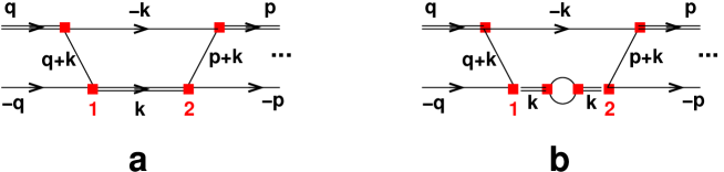
Figure 4: Typical diagrams contributing to the particle-dimer scattering. The double line denotes the dimer, the single line – the particle, and the filled boxes stand for the dimer-two-particle vertex.

In order to demonstrate, how the expression $p^{*}\cot\delta(p^{*})$ emerges, let us consider few diagrams shown in Fig. 4. In particular, in the diagram from Fig. 4a, the energy denominators emerging from the “hopping” of a particle between a particle and a dimer are:

$$\frac{1}{{\bf k}^{2}+{\bf q}^{2}+{\bf k}{\bf q}-mE-i0}\quad\quad\mbox{and}\quad\quad\frac{1}{{\bf k}^{2}+{\bf p}^{2}+{\bf k}{\bf p}-mE-i0}\,,$$ (49)

whereas the factors in the dimer-two-particle vertices (marked as 1 and 2 in the figure) are, respectively

$$f_{0}+f_{1}\biggl{(}{\bf q}+\frac{\bf k}{2}\biggr{)}^{2}+\cdots\quad\quad\mbox{and}\quad\quad f_{0}+f_{1}\biggl{(}{\bf p}+\frac{\bf k}{2}\biggr{)}^{2}+\cdots\,.$$ (50)

Writing

$$f_{0}+f_{1}\biggl{(}{\bf q}+\frac{\bf k}{2}\biggr{)}^{2}+\cdots = ({\bf k}^{2}+{\bf q}^{2}+{\bf k}{\bf q}-mE)+(f_{0}+f_{1}(k^{*})^{2})+\cdots\,,$$

$$f_{0}+f_{1}\biggl{(}{\bf p}+\frac{\bf k}{2}\biggr{)}^{2}+\cdots = ({\bf k}^{2}+{\bf p}^{2}+{\bf k}{\bf p}-mE)+(f_{0}+f_{1}(k^{*})^{2})+\cdots\,,$$ (51)

where $(k^{*})^{2}=mE-\frac{3}{4}\,{\bf k}^{2}$, it is immediately seen that the first term in the above expressions cancels with the pertinent energy denominators. The resulting expression has exactly the form obtained by inserting the local particle-dimer coupling in the diagram. Consequently, it can be removed by redefining the couplings $h_{0},h_{2},\ldots$. The remaining piece contains the factor $f^{2}((k^{*})^{2})$, where $f((k^{*})^{2})=f_{0}+f_{1}(k^{*})^{2}+\cdots$. Moreover, the same factor $f((k^{*})^{2})$ emerges from the diagram Fig. 4b as well – here one may use dimensional regularization to regulate the loop, so the remainder leads to the no-scale integrals and explicitly vanishes (albeit the result, of course, does not depend on the regularization). To summarize, in the case without derivative interactions, the dimer propagator was given by

$$\frac{f_{0}^{2}}{\sigma}+\frac{f_{0}^{4}}{\sigma^{2}}\,I(k^{*})+\cdots=\frac{1}{\sigma f_{0}^{-2}-I(k^{*})}\propto\frac{1}{-a^{-1}-ik^{*}}\,,$$ (52)

where $I(k^{*})\propto ik^{*}$ denotes the loop integral in Fig. 4b with no derivative vertices. If there are derivative vertices present, the above series is modified:

$$\frac{f^{2}((k^{*})^{2})}{\sigma}+\frac{f^{4}((k^{*})^{2})}{\sigma^{2}}\,I(k^{*})+\cdots=\frac{1}{\sigma f^{-2}((k^{*})^{2})-I(k^{*})}\propto\frac{1}{k^{*}\cot\delta(k^{*})-ik^{*}}\,.$$ (53)

An important remark is in order. Usually, in the calculations, the quantity $p\cot\delta(p)$ is approximated by the first few terms in the effective-range expansion. This may lead to the emergence of the spurious poles in the dimer propagator, which lie far outside the region of applicability of the effective-range expansion, and which may render the numerical solution of the scattering equation unstable. In order to circumvent this problem, e.g., in Ref. Bedaque:1998km ; Hammer:2001gh ; Ji:2011qg ; Ji:2012nj a perturbative expansion of the dimer propagator in the effective radius has been proposed. A similar problem might also arise in a finite-volume case, which is our primary concern in this paper. Here we assume that this problem has already been addressed and solved in the infinite volume – e.g., by finding a proper parameterization for $p\cot\delta(p)$ which, at small values of $p$, reproduces the effective-range expansion to a given order, but has a reasonable behavior at large $p^{2}$ and does not lead to spurious poles in the dimer propagator.

II.7 Short summary: three-body problem in the infinite volume

The main features of the three-body problem in the infinite volume can be summarized as follows:

• All physical observables in the three-particle sector at low energies are parameterized in terms of the two-particle $C_{0},C_{2},\ldots$ and three-particle $D_{0},D_{2},\ldots$ couplings. Using equations of motion for reducing number of the independent couplings does not change the observables. The usual power counting applies in the two- and three-particle sector.

• The particle-dimer picture is not an approximation but an equivalent language for the description of the three-particle dynamics. In this picture, one trades the couplings $D_{0},D_{2}$ for the couplings $h_{0},h_{2},\ldots$. In order to incorporate the higher partial waves, dimers with arbitrary (integer) spin should be incorporated.

• The three-body scattering $T$-matrix, which contains information about all physical observables in the three-particle sector, can be expressed in terms of the particle-dimer scattering amplitude ${\cal M}$, which obeys the equation (45), modified in the presence of derivative couplings. Note that the quantity $\tau({\bf k};E)$ in this equation is already parameterized in terms of the physical observables (phase shift) and does not explicitly depend on the regularization used.

III Finite volume

III.1 Strategy

In the previous section, we have thoroughly considered the formulation of the three-particle problem in the infinite volume and have demonstrated that the particle-dimer picture provides an equivalent description of this problem. The reason why we have done this is simple – we will show that the quantization condition can be obtained almost immediately and in an absolutely transparent manner, assuming that the three-momenta in a finite volume are quantized.

The main question here is the choice of an appropriate set of physical observables (parameters), which should be determined from the measured finite volume spectrum. As mentioned before, the previous attempts in the literature were focused on splitting the equations in a finite volume into the infinite-volume part and the rest. We believe that the most convenient choice of the parameters is provided by the low-energy couplings themselves – once these couplings are determined on the lattice, the particle-dimer scattering amplitude can be constructed by solving the scattering equation in the infinite volume.

Let us explain the procedure in more detail. The “scattering amplitude” in a finite volume is determined by the equation

$${\cal M}_{L}({\bf p},{\bf q};E)=Z({\bf p},{\bf q};E)+\frac{8\pi}{L^{3}}\sum\limits_{\bf k}^{\Lambda}\,Z({\bf p},{\bf k};E)\tau_{L}({\bf k};E){\cal M}_{L}({\bf k},{\bf q};E)\,,$$ (54)

where ${\bf k}=\frac{2\pi}{L}\,{\bf n}\,,~{}{\bf n}\in\mathbb{Z}^{3}$ is a quantized three-momentum in a finite volume and

$$\tau^{-1}_{L}({\bf k};E)=k^{*}\cot\delta(k^{*})+S({\bf k},(k^{*})^{2})\,,$$ (55)

where

$$S({\bf k},(k^{*})^{2})=-\frac{4\pi}{L^{3}}\sum_{\bf l}\frac{1}{{\bf k}^{2}+{\bf l}^{2}+{\bf k}{\bf l}-mE}\,.$$ (56)

This sum diverges in the ultraviolet and needs to be regularized and renormalized. The simplest way to do this is to perform a subtraction at some $(k^{*})^{2}=-\mu^{2}<0$ (one subtraction suffices, but more subtractions lead to a faster convergence). Then, we get

$$S({\bf k},(k^{*})^{2})=\bigl{[}S({\bf k},(k^{*})^{2})-S({\bf k},-\mu^{2})\bigr{]}+S({\bf k},-\mu^{2})\,.$$ (57)

The first term in brackets is finite. The second term is equal to

$$S({\bf k},-\mu^{2})=-\frac{4\pi}{L^{3}}\sum_{\bf l}\frac{1}{\bigl{(}{\bf l}+{\bf k}/2\bigr{)}^{2}+\mu^{2}}=\mu-\sum_{{\bf n}\neq{\bf 0}}\frac{1}{nL}\,\exp\biggl{(}-\frac{i}{2}\,L{\bf k}{\bf n}-nL\mu\biggr{)}\,,$$ (58)

where $n=|{\bf n}|$ and we have used Poisson’s summation formula. Note that the ultraviolet divergence in the above expression can be tamed, e.g., by using dimensional regularization. Note also that the equation (54) was used earlier in Refs. Kreuzer:2010ti ; Kreuzer:2009jp ; Kreuzer:2008bi ; Kreuzer:2012sr to calculate the spectrum of the three-body bound states in a finite volume numerically.

Now, our strategy for the analysis of data in the three-particle sector can be formulated as follows:

1. Consider first the two-particle sector, extract the phase shift $\delta(p)$ at different momenta by using the Lüscher equation. Parameterize the function $p\cot\delta(p)$ so that it fits the lattice data and does not lead to spurious poles at large momenta.

2. Fix the cutoff $\Lambda$. Truncate the partial-wave expansion (consider dimers with a spin below some fixed value). Fit the spectrum in the three-particle sector, using $h_{0},h_{2},\ldots$ as free parameters. Repeat this until the fit does not improve anymore by adding parameters.

3. Solve the equations in the infinite volume by using the same values of the parameters and the same cutoff $\Lambda$. Calculate different cross sections, bound-state energies, etc.

The proposed scheme has apparent advantages with respect to the ones proposed in the literature. First of all, it is extremely simple. For example, since we do not want to single out the scattering amplitude in the infinite volume, we do not need to introduce a “smooth cutoff” on the momentum ${\bf l}$ in Eq. (56). Furthermore, the procedure is systematic: the particle-dimer coupling constants $h_{0},h_{2},\ldots$, corresponding to a dimer with a fixed spin, obey the usual counting rules. At the lowest order in the momentum expansion it is just one constant $h_{0}$ for the scalar dimer, which describes the whole three-body spectrum. Finally, the minimal set of couplings is observable, in the sense that they can be uniquely determined from matching to the on-shell $T$-matrix.

In view of the above discussion, the fundamental statement that the finite-volume energy spectrum is determined solely by the three-body $S$-matrix, can be rephrased as follows: the off-shell couplings (like $D_{4}^{\prime\prime}$ considered in the previous section) have no impact on the finite-volume spectrum. This statement can be checked immediately by using exactly the same diagrammatic technique as in the previous section. Indeed, using the no-scale argument, we have proven that $D_{4}^{\prime\prime}$ does not enter the on-shell three-body $T$-matrix. The finite-volume counterpart of this $T$-matrix, which is defined by the same set of Feynman integrals with 3-momentum integrations replaced by sums, determines the spectrum of the three-body system in a finite volume. Namely, its poles correspond to the energy levels. The no-scale integrals in a finite volume also give vanishing contribution (to be more precise, the contribution from the off-shell LECs will be exponentially suppressed $\propto\exp(-ML)$, where the scale $M\sim m$ is much larger than typical non-relativistic momenta). Thus, the fundamental statement from Refs. Polejaeva:2012ut ; Hansen:2014eka looks almost trivial in the new framework.

III.2 Application

In order to demonstrate, how the proposed framework works in practice, we have done a simple exercise. We have restricted ourselves to the scalar dimer and neglected derivative couplings, both in the two-particle and in the three-particle sectors. Thus, for a fixed parameter $\Lambda$, we have two free parameters – the two-body scattering length $a$ and the particle-dimer coupling $h_{0}(\Lambda)$ which can be traded for $H_{0}(\Lambda)$, see subsection II.6. Hence, we want to find the poles of the amplitude ${\cal M}_{L}$, defined by the Eq. (54), where Eq. (55) takes the form

$$\tau^{-1}_{L}({\bf k};E)=-a^{-1}+S({\bf k},(k^{*})^{2})\,,$$ (59)

and

$$Z({\bf p},{\bf q};E)=\frac{1}{-mE+{\bf p}^{2}+{\bf q}^{2}+{\bf p}{\bf q}}+\frac{H_{0}(\Lambda)}{\Lambda^{2}}\,.$$ (60)

In the vicinity of a pole $E=E_{n}$, the amplitude ${\cal M}_{L}$ factorizes

$${\cal M}_{L}({\bf p},{\bf q};E)=\frac{{\cal F}({\bf p}){\cal F}({\bf q})}{E-E_{n}}+\mbox{regular terms.}$$ (61)

Consequently, the spectrum will be determined from the following homogeneous equation:

$${\cal F}({\bf p})=\frac{8\pi}{L^{3}}\,\sum_{\bf q}^{\Lambda}Z({\bf p},{\bf q};E)\tau_{L}({\bf q};E){\cal F}({\bf q})\,.$$ (62)

Next, we would like to perform a partial-wave expansion in this equation. Note that, since the rotation symmetry is broken down by the cubic lattice, a mixing of the partial waves will occur. Using the so-called cubic harmonics, the maximal diagonalization of the matrix equation can be achieved. In doing so, we shall use the general formalism described in Refs. Bernard:2008ax ; Gockeler:2012yj The final result coincides with that of Ref. Kreuzer:2012sr .

We start with the expanding of $Z$ and ${\cal F}$ in partial waves

$$Z({\bf p},{\bf q};E) = 4\pi\sum_{lm}Y_{lm}(\hat{p})Z_{l}(p,q;E)Y^{*}_{lm}(\hat{q})\,,$$

$${\cal F}({\bf p}) = \sqrt{4\pi}\sum_{lm}Y_{lm}(\hat{p}){\cal F}_{lm}(p)\,,$$ (63)

where $\hat{p},\hat{q}$ are unit vectors in the direction of ${\bf p},{\bf q}$, and $Y_{lm}$ denotes spherical functions. Since the spherical symmetry is broken, ${\cal F}_{lm}$ depends on $m$. Further,

$$Z_{l}(p,q;E)=-\frac{1}{2pq}\,\mbox{Re}\,Q_{l}\biggl{(}\frac{mE-p^{2}-q^{2}}{pq}\biggr{)}+\frac{H_{0}(\Lambda)}{\Lambda^{2}}\,\delta_{l0}\,,$$ (64)

where $Q_{l}(z)=\frac{1}{2}\,\int_{-1}^{1}dx\frac{P_{l}(x)}{z-x}$ is the Legendre function of the second kind. In particular,

$$Z_{0}(p,q;E)=\frac{1}{2pq}\,\ln\biggl{|}\frac{p^{2}+pq+q^{2}-mE}{p^{2}-pq+q^{2}-mE}\biggr{|}+\frac{H_{0}(\Lambda)}{\Lambda^{2}}\,.$$ (65)

The equation (62) can be now rewritten in the form

$${\cal F}_{lm}(p)=\sum_{q}^{\Lambda}\sum_{l^{\prime}m^{\prime}}Z_{l}(p,q;E)R_{lm,l^{\prime}m^{\prime}}(q;E){\cal F}_{l^{\prime}m^{\prime}}(q)\,,$$ (66)

where

$$R_{lm,l^{\prime}m^{\prime}}(q;E)=\frac{8\pi}{L^{3}}\,\sum_{|{\bf q}|=q}Y^{*}_{lm}(\hat{q})\tau_{L}({\bf q};E)Y_{l^{\prime}m^{\prime}}(\hat{q})\,,$$ (67)

and $p,q$ take the discrete values: $p,q=\frac{2\pi}{L}\,\sqrt{n_{1}^{2}+n_{2}^{2}+n_{3}^{2}}\,,~{}n_{1},n_{2},n_{3}\in\mathbb{Z}$.

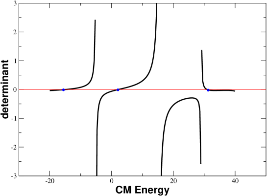
Figure 5: The determinant from Eq. (74). The values of the parameters are $\Lambda a=225$ $L/a=1$, while the shaded blobs correspond to the position of the energy levels.

The system of the homogeneous linear equations (66) has a solution if and only if its determinant vanishes. Consequently, the quantization condition takes the form

$$\det\biggl{(}\delta_{ll^{\prime}}\delta_{mm^{\prime}}\delta_{pq}-Z_{l}(p,q;E)R_{lm,l^{\prime}m^{\prime}}(q;E)\biggr{)}=0\,.$$ (68)

We see explicitly that partial-wave mixing occurs in the quantization condition due to the lost rotational symmetry. It is still possible to block-diagonalize this equation, using the remnant cubic symmetry on the lattice. The basis vectors of the irreducible representations of the cubic group are given by the linear combinations of those of the rotation group Bernard:2008ax ; Gockeler:2012yj

$$|\Gamma\alpha ln\rangle=\sum_{m}c^{\Gamma\alpha n}_{lm}|lm\rangle\,.$$ (69)

Here, $\Gamma$ denotes one of the five irreducible representations $A_{1},A_{2},E,T_{1},T_{2}$ of the cubic group, $n=1,\ldots N(\Gamma,l)$, where $N(\Gamma,l)$ is the number of occurrences of $\Gamma$ in the irreducible representation $D^{l}$ of the rotation group, and $\alpha=1,\ldots\mbox{dim}(\Gamma)$ labels the basis vectors in the irreducible representation $\Gamma$. Further, $c^{\Gamma\alpha n}_{lm}$ are Clebsch-Gordan coefficients. Next, we define

$$R^{\Gamma\Gamma^{\prime}}_{ln\alpha,l^{\prime}n^{\prime}\alpha^{\prime}}(q;E)=\sum_{mm^{\prime}}(c^{\Gamma\alpha n}_{lm})^{*}R_{lm,l^{\prime}m^{\prime}}(q;E)c^{\Gamma^{\prime}\alpha^{\prime}n^{\prime}}_{l^{\prime}m^{\prime}}=\delta_{\Gamma\Gamma^{\prime}}\delta_{\alpha\alpha^{\prime}}R^{\Gamma}_{ln,l^{\prime}n^{\prime}}(q;E)\,,$$ (70)

where the last equality was obtained by using Schur’s lemma. Using the orthogonality of the Clebsch-Gordan coefficients, Eq. (68) can be rewritten as follows:

$$\det\biggl{(}\delta_{nn^{\prime}}\delta_{ll^{\prime}}\delta_{pq}-Z_{l}(p,q;E)R^{\Gamma}_{ln,l^{\prime}n^{\prime}}(q;E)\biggr{)}=0\,.$$ (71)

For simplicity, let us restrict ourselves to the S-waves $l=l^{\prime}=0$. Then, only $\Gamma=A_{1}$ appears in the above expansion and we get

$$\det\biggl{(}\delta_{pq}-Z_{0}(p,q;E)R^{A_{1}}(q;E)\biggr{)}=0\,,$$ (72)

where

$$R^{A_{1}}(q)=\frac{2}{L^{3}}\,\sum_{|{\bf q}|=q}\tau_{L}({\bf q};E)\,.$$ (73)

The matrix can be symmetrized, leading to the eigenvalue equation

$$\det\biggl{(}s(p;E)\delta_{pq}-\sqrt{|R^{A_{1}}(p;E)|}Z_{0}(p,q;E)\sqrt{|R^{A_{1}}(q;E)|}\biggr{)}=0\,,$$ (74)

where $s(p;E)=R^{A_{1}}(q;E)/|R^{A_{1}}(q;E)|$.

The equation (74) can be solved numerically. The square matrix is finite, since $p,q$ are both bound by $\Lambda$. We choose the parameters as in Ref. Kreuzer:2012sr . First of all, we take $m=1$. Further, the cutoff $\Lambda$ is fixed through the two-body scattering length, $a$, by $\Lambda a=225$. Finally, we require that the energy of the bound state in the infinite volume is equal to $E_{\infty}=-10(ma^{2})^{-1}$. This fixes the coupling constant $H_{0}=0.1925$. Calculating now the determinant in Eq. (74) as a function of $E$, one may find the discrete values of $E=E_{1},E_{2},\ldots$, where this function crosses the horizontal axis. Repeating the calculations at different values of the box size $L$, one gets the volume-dependent spectrum $E_{1}(L),E_{2}(L),\ldots$. Figure 5 shows the results of calculation of the determinant at one particular value of $L$, whereas Fig. 6 displays the volume-dependent spectrum – both below and above three-particle threshold.

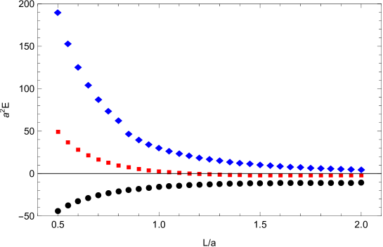
Figure 6: The dependence of the energy levels on the box size for a fixed value $\Lambda a=225$. The levels both below and above the three-particle threshold are considered. The behavior of the subthreshold level agrees well with the result of Ref. Kreuzer:2012sr .

What does one learn from these results? For a fixed value of $\Lambda$ and $L$, the spectrum is determined by a limited set of the parameters $H_{0},H_{2},\ldots$ (we imply that $C_{0},C_{2},\ldots$ are determined in the two-particle sector). In the simplest case considered here, this is just one parameter $H_{0}$. For the analysis of the lattice data, one has to calculate the energy levels as a function of $H_{0}$ and fit to the existing data. If this is not enough, one has to include derivative couplings and dimers with higher spin, until the quality of fit does not change. We stress once more that this is a systematic prescription – the derivative couplings obey counting rules and are less and less relevant at low energies. The same is true for the partial-wave truncation – higher partial ways give little contribution at low energies.

To summarize, the framework described above gives a simple and systematic tool to analyze the lattice data in the three-particle sector.

IV Comparison with existing approaches

Several groups have previously addressed the three-particle problem in a finite volume. In this section, we would like to briefly review these approaches and clarify the relation to the approach which was considered in the present paper.

We start from Refs. Hansen:2014eka ; Hansen:2015zga ; Briceno:2017tce , where the three-particle quantization condition has been obtained. That derivation has been carried out looking for the poles of the three-particle Green function in a finite volume. Since we have explicitly demonstrated that the particle-dimer picture is equivalent to the three-particle description, and since our formalism also extracts the poles of the particle-dimer scattering amplitude, it is no wonder that, diagrammatically, both quantization conditions are the same. This will be explicitly shown below.

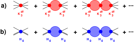
Figure 7: a) The three-particle Green function and b) The particle-dimer Green function: insertion of the three particle/particle-dimer couplings. The shaded blobs contain only self-energy insertions and particle “hopping,” see Fig. 8.

First, note that the quantity $K_{3}^{\sf df}$, defined in Ref. Hansen:2014eka , is a counterpart of our $H_{0}+\ldots$ (a more precise statement will follow). The three-particle Green function in the framework of Refs. Hansen:2014eka ; Hansen:2015zga ; Briceno:2017tce and the particle-dimer Green function in our approach are shown in Figs. 7a and 7b, respectively. It is clear that one may relate these two quantization conditions, if the corresponding shaded blobs (containing only pair interactions), or only two-particle dimer interactions, are related to each other. These blobs are depicted in Figs. 8a and 8b, respectively.

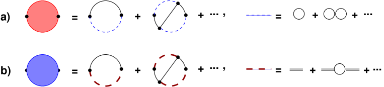
Figure 8: The shaded blobs in Fig. 7 describe the propagation of the spectator particle and a) a pair of particles interacting with each other through contact interactions, or b) a dressed dimer. These two lines are connected by particle “hopping.”

The blob in Fig.8b contains two-types of diagrams: self-energy insertions into the dimer line, and the particle “hopping.” In order to get a feeling, let us calculate few diagrams shown in Fig. 9 (for simplicity, let us restrict ourselves to the non-derivative couplings only). Using split dimensional regularization in the first term, it can be shown that

$${\cal M}_{a} = \int\sum_{~{}l}\frac{1}{\sigma}\,\frac{1}{\frac{{\bf l}^{2}}{2m}-E+l_{0}-i0}=0\,,$$

$${\cal M}_{b} = \frac{1}{2}\,f_{0}^{2}\int\sum_{~{}l}\int\sum_{~{}k}\frac{1}{\sigma^{2}}\frac{1}{\frac{{\bf l}^{2}}{2m}-E+l_{0}-i0}\,\frac{1}{\frac{{\bf k}^{2}}{2m}-k_{0}-i0}\,\frac{1}{\frac{({\bf l}+{\bf k})^{2}}{2m}-l_{0}+k_{0}-i0}$$

$$= \frac{1}{2}\,f_{0}^{2}\frac{1}{L^{3}}\sum_{\bf l}\frac{1}{L^{3}}\sum_{\bf k}\frac{1}{\frac{1}{m}\,({\bf l}^{2}+{\bf k}^{2}+{\bf l}{\bf k})-E}\,,$$

$${\cal M}_{c} = f_{0}^{2}\int\sum_{~{}l}\int\sum_{~{}k}\frac{1}{\sigma^{2}}\frac{1}{\frac{{\bf l}^{2}}{2m}-P_{0}+l_{0}-i0}\,\frac{1}{\frac{{\bf k}^{2}}{2m}-P_{0}+k_{0}-i0}\,\frac{1}{\frac{({\bf l}+{\bf k})^{2}}{2m}-P_{0}-k_{0}+l_{0}-i0}$$ (75)

$$= f_{0}^{2}\frac{1}{L^{3}}\sum_{\bf l}\frac{1}{L^{3}}\sum_{\bf k}\frac{1}{\frac{1}{m}\,({\bf l}^{2}+{\bf k}^{2}+{\bf l}{\bf k})-E}\,,$$

and so on, where

$$\int\sum_{~{}l}(\cdots)=\int\frac{dl_{0}}{2\pi i}\frac{1}{L^{3}}\sum_{\bf l}(\cdots)\,.$$ (76)

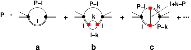
Figure 9: The lowest-order diagrams, contributing to the shaded blob in the particle-dimer picture, see Fig. 8b. The double line depicts a dimer and the single line – a particle.

Denoting the self-energy insertion by $J$ and the “hopping” diagram by $-G$, and defining $a_{0}=\frac{1}{2}\,f_{0}^{2}$, the blob shown in Fig. 8b can be symbolically written down as

$${\cal M}_{dimer} = (a_{0}^{2}J+a_{0}^{3}J^{2}+\cdots)-(a_{0}+a_{0}^{2}J+\cdots)G(a_{0}+a_{0}^{2}J+\cdots)+\cdots$$ (77)

$$= \frac{a_{0}^{2}J}{1-a_{0}J}-\frac{a_{0}J}{1-a_{0}J}\,G\frac{a_{0}J}{1-a_{0}J}+\cdots\,.$$

Next, we prove a key equality that allows one to transform this expression into the form given in Refs. Hansen:2014eka ; Hansen:2015zga ; Briceno:2017tce . It is seen from Eq. (IV) that, if $G$ appears on the left or on the right of all insertions, then $G$ can be replaced by $-2J$. This is a general property which is valid for any number of insertions. Indeed, as seen from Fig. 9, contracting the free dimer propagator to a point, topologically there is no difference between the diagrams Fig. 9b and Fig. 9c. This will remain true, if any number of insertions (both $J$ and $G$) are placed on the left or on the right (but not both!).

Now, we are able to demonstrate that our quantization condition is equivalent to that of Refs. Hansen:2014eka ; Hansen:2015zga ; Briceno:2017tce . To this end, we introduce the following notations for the two- and three-body amplitudes:

$${\cal M}_{2}=\frac{a_{0}}{1-a_{0}J}\,,\quad\quad{\cal M}_{3}={\cal M}_{2}-{\cal M}_{2}G{\cal M}_{3}\,.$$ (78)

Using these definitions and replacing $G$ by $(-2J)$ on the left and on the right in all terms, after lengthy but straightforward algebraic transformations (see appendix A), we obtain

$${\cal M}_{dimer}=9a_{0}^{2}\biggl{(}\frac{1}{3}\,J+J{\cal M}_{3}J\biggr{)}\,.$$ (79)

This is exactly the same expression as in Refs. Hansen:2014eka ; Hansen:2015zga ; Briceno:2017tce .

Though we have just demonstrated that diagrammatically both quantization conditions are equivalent, some differences remain. In the Refs. Hansen:2014eka ; Hansen:2015zga ; Briceno:2017tce a smooth cutoff, introduced first in Ref. Polejaeva:2012ut , has been used both in the self-energy insertion $J$ as well as on the sum over the momenta ${\bf q}$ of the spectator particle. Denoting the cutoff function by $H({\bf q})$, the sum over ${\bf q}$ is given by

$$\frac{1}{L^{3}}\sum_{\bf q}(\cdots)=\frac{1}{L^{3}}\sum_{\bf q}\bigl{[}H({\bf q})+(1-H({\bf q}))\bigr{]}(\cdots)\,.$$ (80)

The cutoff function is chosen so that $(1-H({\bf q}))=0$, if $mE>\frac{3}{4}\,{\bf q}^{2}$ (in the non-relativistic limit). This means that the second term in this equation is smooth and the sum can be replaced by the integral. Consider now Eq. (54). Symbolically, it can be written as

$${\cal M}_{L}=Z+\sum_{\bf q}H({\bf q})Z\tau_{L}{\cal M}_{L}+\int_{\bf q}(1-H({\bf q}))Z\tau{\cal M}_{L}\,,$$ (81)

where $\tau=\lim_{L\to\infty}\tau_{L}$. Defining now the “non-standard $K$-matrix” in the context of the particle-dimer picture

$${\cal M}_{H}=Z+\int_{\bf q}(1-H({\bf q}))Z\tau{\cal M}_{H}\,,$$ (82)

we arrive at

$${\cal M}_{L}={\cal M}_{H}+\sum_{\bf q}H({\bf q}){\cal M}_{H}\tau_{L}{\cal M}_{L}\,.$$ (83)

The quantization condition that can be obtained from this equation has exactly the same form as in Refs. Hansen:2014eka ; Hansen:2015zga ; Briceno:2017tce . Consequently, the main difference with our approach consists in moving down the cutoff from $\Lambda$. The advantage of this is that the system of the linear equations that determines the finite-volume spectrum is lower-dimensional, since the maximum momentum is determined by the cutoff. However, one has to introduce the quantity ${\cal M}_{H}$ instead of a single parameter $H_{0}$, and further find the conventional infinite-volume $K$ matrix by solving an integral equation involving ${\cal M}_{H}$. All this renders the formalism complicated and difficult to apply to the analysis of data.

In addition, Ref. Hansen:2014eka it was argued that the introduction of the cutoff $H$ allows one to always define the Lorentz boost, bringing the pair of two interacting particles to the rest frame. Namely, the cutoff excludes the region, where the total momentum squared of two particles is negative. While the latter statement is certainly true, in this case the problem is merely shifted to the calculation of ${\cal M}_{H}$. Note also that the same problem would arise in the three-body problem in the infinite volume as well, leading to the conclusion that one can not move the cutoff above some fixed point determined by kinematics. The fact is that, even if the boost is undefined, the two-body scattering amplitude is defined for all momenta, given the non-relativistic Lagrangian, in which the couplings are matched to the effective-range expansion parameters defined in the CM frame. In the relativistic case, it is convenient to use the covariant version of the non-relativistic effective field theory Colangelo:2006va ; Gasser:2011ju , which provides explicitly Lorentz-invariant expression of the two-body amplitudes.

Having considered Refs. Hansen:2014eka ; Hansen:2015zga ; Briceno:2017tce in detail, we next turn to Ref. Polejaeva:2012ut . The three-particle Green function, considered here, contains the same set of diagrams as in Refs. Hansen:2014eka ; Hansen:2015zga ; Briceno:2017tce (including, in particular, two-to-three transitions as well). The final answer is given in a form of a system of linear equations, and the quantization condition can straightforwardly be obtained by declaring the determinant of this system equal to zero. What is different, is the cutoff on the spectator momentum, which is now moved down to zero (the cutoff in the self-energy diagram stays where it was before). Since Lüscher’s regular summation theorem in the spectator momentum ${\bf q}$ can not be applied everywhere, the dimensionality of the equations is the same as in Refs. Hansen:2014eka ; Hansen:2015zga ; Briceno:2017tce and, because the “non-standard $K$-matrix” has to be introduced, this formalism is very complicated as well.

Finally, the formalism constructed in Ref. Briceno:2012rv is based on the particle-dimer picture and is close to the one we are using here. The authors go further and replace the exact dimer propagator by a sum over the finite-volume two-particle poles (there is always a finite number thereof, limited by kinematics) and the rest, that can be calculated in the infinite volume. This effectively amounts to introducing a cutoff on the spectator momentum, defined by the lowest-lying pole. All above discussion also applies here.

To summarize, the alternative approaches discussed in this section separate finite- and infinite-volume contributions in the three-particle amplitude. This leads to the introduction of the quantities like the “unconventional $K$-matrix” that render the formalism rather complicated. Instead of this, we advocate for solving the particle-dimer equation in a finite volume directly and fitting the low-energy couplings to the measured spectrum. Note also that, since all these unconventional $K$-matrices should be low-energy polynomials (the low-energy region is cut off in the integral equation), one could expand these quantities in momenta and arrive at equations which are formally similar to our equations but are using a smooth cutoff at $\Lambda\sim m$. Exactly the same result can be obtained in much more direct way, lowering the cutoff $\Lambda$ in our equations and taking into account the fact that the couplings run with $\Lambda$.

V Conclusions

In this paper, we propose an effective field theory framework, which can be used to analyze the three-particle spectrum on the lattice.

• The crucial point consists in the choice of a convenient set of parameters that can be fit to the lattice data. Within our framework, this set is formed by the particle-dimer couplings (effective couplings in the two-particle sector should be determined separately). Any physical observable can be determined, using the set of couplings determined on the lattice.

• The proposed approach is hardly new. However, it was important to realize that it is algebraically equivalent to existing approaches, known in the literature. Moreover, we have demonstrated that it is systematic, much simpler in use than the existing approaches, and can be applied for data analysis even when only a few data points are available.

• As an illustration, we have used this approach to calculate the energy spectrum (both below and above the three-particle threshold) by using the input values of the couplings. As a further illustration, note that this approach was successfully used 1 to reproduce the result of Ref. Meissner:2014dea on the three-body bound state energy shift in a finite volume, as well as to study the role of the three-particle force and the generalization of the above result beyond the unitary limit.

• In order to emphasize the main conceptual problem and its solution, technical details like relativistic kinematics, higher partial waves, etc. have been left out. These will be included in future publications.

• The treatment in this paper rests on a particular form of the effective field theory that describes the three-particle system in a finite volume. In the case of the nucleons, for example, one may have to take into account the pion exchanges between nucleons explicitly leading to a different “chiral” effective field theory. This does not, however, change the underlying idea of our proposal – considering a given effective field theory (relativistic or non-relativistic) in a finite volume, calculating the spectrum numerically and fitting the low-energy constants to the spectrum. Note also that a very similar strategy is pursued within the framework of the unitary ChPT in a finite volume oset ; Doring-scalar ; oset-in-a-finite-volume , which is used in the analysis of data in the two-particle sector. A possible alternative scheme in the three-body sector based on the isobar approximation was recently discussed in Ref. Mai:2017vot .

Appendix A Derivation of Eq. (79)

The equation (79) can be obtained by transforming the expression (77) as

$$a_{0}^{-2}{\cal M}_{dimer} = J\frac{1}{1-a_{0}J}-\frac{1}{1-a_{0}J}\,\biggl{\{}G-G\frac{a_{0}}{1-a_{0}J}G+G\frac{a_{0}}{1-a_{0}J}\,G\frac{a_{0}}{1-a_{0}J}G-\cdots\biggr{\}}\frac{1}{1-a_{0}J}$$ (84)

$$= J\frac{1}{1-a_{0}J}-\frac{1}{1-a_{0}J}\,\biggl{\{}G-G({\cal M}_{2}-{\cal M}_{2}G{\cal M}_{2}+\cdots)G\biggr{\}}\frac{1}{1-a_{0}J}$$

$$= J\frac{1}{1-a_{0}J}-\frac{1}{1-a_{0}J}\,\biggl{\{}G-G{\cal M}_{3}G\biggr{\}}\frac{1}{1-a_{0}J}$$

$$= J\frac{1}{1-a_{0}J}-G-\frac{a_{0}J}{1-a_{0}J}\,G-G\frac{a_{0}J}{1-a_{0}J}-\frac{a_{0}J}{1-a_{0}J}\,G\frac{a_{0}J}{1-a_{0}J}$$

$$+ G{\cal M}_{3}G+\frac{a_{0}J}{1-a_{0}J}\,G{\cal M}_{3}G+G{\cal M}_{3}G\frac{a_{0}J}{1-a_{0}J}+\frac{a_{0}J}{1-a_{0}J}\,G{\cal M}_{3}G\frac{a_{0}J}{1-a_{0}J}\,.$$

In some terms of the above expression, $G$ appears on the very left or on the very right. Here, one may replace $G$ with $-2J$, arriving at the following expression

$$a_{0}^{-2}{\cal M}_{dimer} = J\frac{1}{1-a_{0}J}+2J+\frac{4a_{0}J^{2}}{1-a_{0}J}-\frac{a_{0}J}{1-a_{0}J}\,G\frac{a_{0}J}{1-a_{0}J}$$ (85)

$$+ 4J{\cal M}_{3}J-\frac{2a_{0}J}{1-a_{0}J}\,G{\cal M}_{3}J-J{\cal M}_{3}G\frac{2a_{0}J}{1-a_{0}J}+\frac{a_{0}J}{1-a_{0}J}\,G{\cal M}_{3}G\frac{a_{0}J}{1-a_{0}J}$$

$$= J\biggl{\{}{\cal M}_{2}G{\cal M}_{3}G{\cal M}_{2}-{\cal M}_{2}G{\cal M}_{2}+4{\cal M}_{3}-2{\cal M}_{2}G{\cal M}_{3}-2{\cal M}_{3}G{\cal M}_{2}\biggr{\}}J$$

$$+ J\frac{1}{1-a_{0}J}+2J+\frac{4a_{0}J^{2}}{1-a_{0}J}\,.$$

The last term can be replaced by

$$\frac{4a_{0}J^{2}}{1-a_{0}J}=4J{\cal M}_{2}J\,.$$ (86)

Finally, using Eq. (78), we get

$$a_{0}^{-2}{\cal M}_{dimer} = 9J{\cal M}_{3}J+3J-J({\cal M}_{2}J+1)+\frac{J}{1-a_{0}J}=9\biggl{(}\frac{1}{3}J+J{\cal M}_{3}J\biggr{)}\,,$$ (87)

which coincides with Eq. (79)  .

References

- (1) M. Lüscher, Nucl. Phys. B 354 (1991) 531, doi:10.1016/0550-3213(91)90366-6.
-
(2)
M. Lage, U.-G. Meißner and A. Rusetsky,
Phys. Lett. B 681 (2009) 439,
arXiv:0905.0069 [hep-lat]. -
(3)
V. Bernard, M. Lage, U.-G. Meißner and A. Rusetsky,
JHEP 1101 (2011) 019,
arXiv:1010.6018 [hep-lat]. - (4) C. Liu, X. Feng and S. He, JHEP 0507 (2005) 011, arXiv:hep-lat/0504019; Int. J. Mod. Phys. A 21 (2006) 847, arXiv:hep-lat/0508022.
- (5) M. T. Hansen and S. R. Sharpe, Phys. Rev. D 86 (2012) 016007, arXiv:1204.0826 [hep-lat].
- (6) R. A. Briceno and Z. Davoudi, Phys. Rev. D 88 (2013) 094507, arXiv:1204.1110 [hep-lat].
- (7) N. Li and C. Liu, Phys. Rev. D 87 (2013) 014502, arXiv:1209.2201 [hep-lat].
-
(8)
P. Guo, J. Dudek, R. Edwards and A. P. Szczepaniak,
Phys. Rev. D 88 (2013) 014501,
arXiv:1211.0929 [hep-lat]. - (9) J. J. Dudek et al. [Hadron Spectrum Collaboration], Phys. Rev. Lett. 113 (2014) 182001, arXiv:1406.4158 [hep-ph]; D. J. Wilson, J. J. Dudek, R. G. Edwards and C. E. Thomas, Phys. Rev. D 91 (2015) 054008, arXiv:1411.2004 [hep-ph]; J. J. Dudek, R. G. Edwards and D. J. Wilson, arXiv:1602.05122 [hep-ph].
-
(10)
M. Döring, U.-G. Meißner, E. Oset and A. Rusetsky,
Eur. Phys. J. A 47 (2011) 139,
arXiv:1107.3988 [hep-lat]. -
(11)
M. Döring, U.-G. Meißner, E. Oset and A. Rusetsky,
Eur. Phys. J. A 48 (2012) 114,
arXiv:1205.4838 [hep-lat]. -
(12)
A. M. Torres, L. R. Dai, C. Koren, D. Jido and E. Oset,
Phys. Rev. D 85 (2012) 014027,
arXiv:1109.0396 [hep-lat]; M. Döring and U.-G. Meißner, JHEP 1201 (2012) 009,
arXiv:1111.0616 [hep-lat]; M. Döring, M. Mai and U.-G. Meißner, Phys. Lett. B 722 (2013) 185, arXiv:1302.4065 [hep-lat]. - (13) D. R. Bolton, R. A. Briceno and D. J. Wilson, arXiv:1507.07928 [hep-ph].
-
(14)
D. Agadjanov, M. Döring, M. Mai, U.-G. Meißner and A. Rusetsky,
JHEP 1606 (2016) 043,
arXiv:1603.07205 [hep-lat]. - (15) M. T. Hansen, H. B. Meyer and D. Robaina, arXiv:1704.08993 [hep-lat].
-
(16)
N. Ishii et al. [HAL QCD Collaboration],
Phys. Lett. B 712 (2012) 437,
arXiv:1203.3642 [hep-lat]; S. Aoki, Eur. Phys. J. A 49 (2013) 81, arXiv:1309.4150 [hep-lat]. - (17) S. Aoki, PoS LAT 2007 (2007) 002, arXiv:0711.2151 [hep-lat].
-
(18)
S. Aoki, B. Charron, T. Doi, T. Hatsuda, T. Inoue and N. Ishii,
Phys. Rev. D 87 (2013) 034512 arXiv:1212.4896 [hep-lat]; K. Sasaki, S. Aoki, T. Doi, T. Hatsuda, Y. Ikeda, T. Inoue, N. Ishii and K. Murano, arXiv:1504.01717 [hep-lat]. - (19) K. Polejaeva and A. Rusetsky, Eur. Phys. J. A 48 (2012) 67, arXiv:1203.1241 [hep-lat].
- (20) U.-G. Meißner, G.-Rios and A. Rusetsky, Phys. Rev. Lett. 114 (2015) 091602 Erratum: [Phys. Rev. Lett. 117 (2016) 069902], arXiv:1412.4969 [hep-lat].
- (21) P. Guo, Phys. Rev. D 95 (2017) 054508, arXiv:1607.03184 [hep-lat].
- (22) P. Guo and V. Gasparian, arXiv:1701.00438 [hep-lat].
- (23) R. A. Briceno and Z. Davoudi, Phys. Rev. D 87 (2013) 094507, arXiv:1212.3398 [hep-lat].
-
(24)
M. T. Hansen and S. R. Sharpe,
Phys. Rev. D 90 (2014) 116003,
arXiv:1408.5933 [hep-lat]. -
(25)
M. T. Hansen and S. R. Sharpe,
Phys. Rev. D 92 (2015) 114509,
arXiv:1504.04248 [hep-lat]. - (26) M. T. Hansen and S. R. Sharpe, Phys. Rev. D 93 (2016) 014506, arXiv:1509.07929 [hep-lat].
-
(27)
M. T. Hansen and S. R. Sharpe,
Phys. Rev. D 93 (2016) 096006,
arXiv:1602.00324 [hep-lat]. -
(28)
M. T. Hansen and S. R. Sharpe,
Phys. Rev. D 95 (2017) 034501,
arXiv:1609.04317 [hep-lat]. - (29) R. A. Briceño, M. T. Hansen and S. R. Sharpe, arXiv:1701.07465 [hep-lat].
- (30) S. Kreuzer and H.-W. Hammer, Phys. Lett. B 694 (2011) 424, arXiv:1008.4499 [hep-lat].
- (31) S. Kreuzer and H.-W. Hammer, Eur. Phys. J. A 43 (2010) 229, arXiv:0910.2191 [nucl-th].
- (32) S. Kreuzer and H.-W. Hammer, Phys. Lett. B 673 (2009) 260, arXiv:0811.0159 [nucl-th].
- (33) S. Kreuzer and H. W. Grießhammer, Eur. Phys. J. A 48 (2012) 93, arXiv:1205.0277 [nucl-th].
- (34) N. Mathur, Y. Chen, S. J. Dong, T. Draper, I. Horvath, F. X. Lee, K. F. Liu and J. B. Zhang, Phys. Lett. B 605 (2005) 137, arXiv:hep-ph/0306199.
-
(35)
D. Guadagnoli, M. Papinutto and S. Simula,
Phys. Lett. B 604 (2004) 74,
arXiv:hep-lat/0409011. - (36) D. B. Leinweber, W. Melnitchouk, D. G. Richards, A. G. Williams and J. M. Zanotti, Lect. Notes Phys. 663 (2005) 71, arXiv:nucl-th/0406032.
- (37) K. Sasaki, S. Sasaki and T. Hatsuda, Phys. Lett. B 623 (2005) 208, arXiv:hep-lat/0504020.
- (38) K. Sasaki and S. Sasaki, Phys. Rev. D 72 (2005) 034502, arXiv:hep-lat/0503026.
- (39) T. Burch, C. Gattringer, L. Y. Glozman, C. Hagen, D. Hierl, C. B. Lang and A. Schafer, Phys. Rev. D 74 (2006) 014504, arXiv:hep-lat/0604019.
-
(40)
K. F. Liu, Y. Chen, M. Gong, R. Sufian, M. Sun and A. Li,
PoS LATTICE 2013 (2014) 507,
arXiv:1403.6847 [hep-ph]. - (41) M. S. Mahbub, A. O. Cais, W. Kamleh, D. B. Leinweber and A. G. Williams, Phys. Rev. D 82 (2010) 094504, arXiv:1004.5455 [hep-lat].
- (42) B. G. Lasscock, J. N. Hedditch, W. Kamleh, D. B. Leinweber, W. Melnitchouk, A. G. Williams and J. M. Zanotti, Phys. Rev. D 76 (2007) 054510, arXiv:0705.0861 [hep-lat].
- (43) C. B. Lang, L. Leskovec, M. Padmanath and S. Prelovsek, Phys. Rev. D 95 (2017) 014510, arXiv:1610.01422 [hep-lat].
-
(44)
S. R. Beane, W. Detmold, K. Orginos and M. J. Savage,
Prog. Part. Nucl. Phys. 66 (2011) 1,
arXiv:1004.2935 [hep-lat]. -
(45)
S. R. Beane et al. [NPLQCD Collaboration],
Phys. Rev. D 87 (2013) 034506,
arXiv:1206.5219 [hep-lat]. -
(46)
E. Chang et al. [NPLQCD Collaboration],
Phys. Rev. D 92 (2015) 114502,
arXiv:1506.05518 [hep-lat]. -
(47)
E. Epelbaum, H. Krebs, D. Lee and U.-G. Meißner,
Phys. Rev. Lett. 104 (2010) 142501,
arXiv:0912.4195 [nucl-th]. -
(48)
E. Epelbaum, H. Krebs, D. Lee and U.-G. Meißner,
Phys. Rev. Lett. 106 (2011) 192501,
arXiv:1101.2547 [nucl-th]. -
(49)
A. Rokash, E. Epelbaum, H. Krebs, D. Lee and U.-G. Meißner,
J. Phys. G 41 (2014) 015105,
arXiv:1308.3386 [nucl-th]. - (50) S. Elhatisari, D. Lee, G. Rupak, E. Epelbaum, H. Krebs, T. A. Lähde, T. Luu and U.-G. Meißner, Nature 528 (2015) 111, arXiv:1506.03513 [nucl-th].
-
(51)
P. F. Bedaque, H.-W. Hammer and U. van Kolck,
Phys. Rev. Lett. 82 (1999) 463,
arXiv:nucl-th/9809025. -
(52)
P. F. Bedaque, H.-W. Hammer and U. van Kolck,
Nucl. Phys. A 646 (1999) 444,
arXiv:nucl-th/9811046. - (53) H.-W. Hammer and T. Mehen, Phys. Lett. B 516 (2001) 353, arXiv:nucl-th/0105072.
- (54) C. Ji, D. R. Phillips and L. Platter, Annals Phys. 327 (2012) 1803, arXiv:1106.3837 [nucl-th].
- (55) C. Ji and D. R. Phillips, Few Body Syst. 54 (2013) 2317, arXiv:1212.1845 [nucl-th].
-
(56)
V. Bernard, M. Lage, U.-G. Meißner and A. Rusetsky,
JHEP 0808 (2008) 024,
arXiv:0806.4495 [hep-lat]. - (57) M. Gockeler, R. Horsley, M. Lage, U.-G. Meißner, P. E. L. Rakow, A. Rusetsky, G. Schierholz and J. M. Zanotti, Phys. Rev. D 86 (2012) 094513, arXiv:1206.4141 [hep-lat].
-
(58)
G. Colangelo, J. Gasser, B. Kubis and A. Rusetsky,
Phys. Lett. B 638 (2006) 187,
arXiv:hep-ph/0604084. - (59) J. Gasser, B. Kubis and A. Rusetsky, Nucl. Phys. B 850 (2011) 96, arXiv:1103.4273 [hep-ph].
- (60) H.-W. Hammer, J.-Y. Pang and A. Rusetsky, arXiv:1706.07700 [hep-lat].
- (61) M. Mai, B. Hu, M. Döring, A. Pilloni and A. Szczepaniak, arXiv:1706.06118 [nucl-th].