A Cut Discontinuous Galerkin Method for Coupled Bulk-Surface Problems

Abstract

We develop a cut Discontinuous Galerkin method (cutDGM) for a diffusion-reaction equation in a bulk domain which is coupled to a corresponding equation on the boundary of the bulk domain. The bulk domain is embedded into a structured, unfitted background mesh. By adding certain stabilization terms to the discrete variational formulation of the coupled bulk-surface problem, the resulting cutDGM is provably stable and exhibits optimal convergence properties as demonstrated by numerical experiments. We also show both theoretically and numerically that the system matrix is well-conditioned, irrespective of the relative position of the bulk domain in the background mesh.

1 Introduction

In recent years, the analysis and numerical solution of coupled bulk-surface partial differential equations (PDE) have gained a large interests in the fields of computational engineering and scientific computing. Indeed, a number of important phenomena in biology, geology and physics can be described by such PDE systems. A prominent use case are flow and transport problems in porous media when large-scale fracture networks are modeled as 2D geometries embedded into a 3D bulk domain Martin et al. (2005); Formaggia et al. (2013). Another important example is the modeling of cell motility where reaction-diffusion systems on the cell membrane and inner cell are coupled to describe the active reorganization of the cytoskeleton Novak et al. (2007); Rätz (2015). Coupled bulk-surface PDEs arise also naturally when modeling incompressible multi-phase flow problems with surfactants Ganesan and Tobiska (2009); Groß and Reusken (2011); Muradoglu and Tryggvason (2008); Groß and Reusken (2013).

The numerical solution of coupled bulk-surface systems poses several challenges even for modern computational methods. First, one faces a system of coupled PDEs on domains of different topological dimensionality, which needs to be accommodated by the numerical method at hand. Second, extremely complex surface geometries naturally appear in many realistic application scenarios, e.g., when complex fracture networks in porous media models are considered, and thus fast and robust mesh generation becomes a challenge. Moreover, the simulation of complex droplet systems shows that, even if the initial surface geometry is relatively simple, it might evolve significantly over time and thus can undergo large or even topological changes. For traditional discretization methods, a costly remeshing of the computational domain is then the only resort, and the question of how to transfer the computed solution components between different meshes efficiently and accurately becomes an urgent and challenging matter.

As a potential remedy to these challenges, the so-called cut finite element method (CutFEM) has gained a large interest in recent years, see Burman et al. (2015a) for a review. The basic idea is to decouple the description of the geometry as much as possible from the underlying approximation spaces by embedding the geometry of the domain into a fixed background mesh which is also used to construct the finite element spaces for the surface and bulk approximations. In order to obtain a stable method, independent of the position of the geometry in the background mesh, and to handle the potential small cut elements in the analysis, certain stabilization terms are added that provide control of the local variation of the discrete functions. In this work we extend ideas from CutFEM framework developed over the last half a decade to synthesize a novel cut discontinuous Galerkin method (cutDGM) for coupled bulk-surface PDEs.

1.1 Earlier work

The development of the cut finite element framework was initiated by the seminal papers Burman and Hansbo (2010, 2012) considering the weak imposition of boundary conditions for the Poisson problem on unfitted meshes. Shortly after, the idea was picked up by a number of authors to formulate cut finite element methods for the Stokes type problemsBurman and Hansbo (2013); Massing (2012); Massing et al. (2014); Burman et al. (2015b); Guzmán and Olshanskii (2017); Hansbo et al. (2014), the Oseen problem Massing et al. (2016); Winter et al. (2017) and number of related fluid problems, see Schott (2017) for a comprehensive overview.

Prior to the arrival of CutFEMs, unfitted discontinuous Galerkin methods have successfully been employed to solve boundary and interface problems on complex and evolving domains Bastian and Engwer (2009); Saye (2015), including two-phase flows Sollie et al. (2011); Heimann et al. (2013); Müller et al. (2016). In unfitted discontinuous Galerkin method, troublesome small cut elements can be merged with neighbor elements with a large intersection support by simply extending the local finite element basis from the large element to the small cut element. As the inter-element continuity is enforced only weakly, the coupling of the these extended basis functions to additional elements incident with the small cut elements does not lead to an over-constrained system, as it would happen if globally continuous finite element functions were employed. Consequently, unfitted discontinuous Galerkin methods provide an alternative stabilization mechanism to ensure the well-posedness and well-conditioning of the discretized systems. Thanks to their favorable conservation and stability properties, unfitted discontinuous Galerkin methods remain an attractive alternative to continuous CutFEMs, but some drawbacks are the almost complete absence of numerical analysis except for Massjung (2012); Johansson and Larson (2013), the implementational labor to reorganize the matrix sparsity patterns when agglomerating cut elements, and the lack of natural discretization approaches for PDEs defined on surfaces.

For PDEs defined on surfaces, the idea of using the finite element space from the embedding bulk mesh was already formulated and analyzed in Olshanskii et al. (2009), and then further extended to high-order methods Grande and Reusken (2016) and evolving surface problems Olshanskii et al. (2014); Hansbo et al. (2015). A stabilized cut finite element for the Laplace-Beltrami problem were introduced in Burman et al. (2015c) where the additional stabilization cures the resulting system matrix from being ill-conditioned, as an alternative to diagonal preconditioning used in Olshanskii and Reusken (2010). Finally, after the initial work Elliott and Ranner (2013) on fitted finite element discretizations of coupled bulk-surface PDEs, only a few number of corresponding unfitted (continuous) finite element schemes have been formulated, see Burman et al. (2016); Hansbo et al. (2016); Groß et al. (2015).

1.2 Contribution and outline of the paper

In this work, we formulate a novel cut discontinuous Galerkin method for the discretization of coupled bulk-surface problems on a given bounded domain $\Omega$. The strong and weak formulation of a continuous prototype problem are briefly reviewed in Section 2. Motivated by our earlier work Burman et al. (2016), we introduce a cut discontinuous Galerkin method for bulk-surface PDEs in Section 3. The method is employs discontinuous piecewise linear elements on a background mesh consisting of simplices in $\mathbb{R}^{d}$. The boundary $\Gamma$ of the computational domain $\Omega$ is represented by a continuous, piecewise approximation of distance functions associated with $\Gamma$. For both the discrete bulk and surface domain, the active background meshes consist of those elements with a non-trivial intersection with the respective domain. Utilizing the general stabilization framework developed for continuous CutFEMs, we add certain, so-called ghost penalty stabilization in the vicinity of the embedded surface to ensure that the overall cutDGM is stable and its system matrix is well-conditioned. The exact mechanism is further elucidated in Section 4, where short proofs of the coercivity of the bilinear forms introduced in Section 3 are given. We also demonstrate that the condition number of the (properly rescaled) system matrix scales like $\mathcal{O}(h^{-2})$. All theoretical results hold with constants independent of the position of the domain relative to the background mesh.

While a full a priori analysis of the proposed method is beyond the limited scope of this work, we perform a convergence rate study in Section 5 instead, demonstrating the optimal approximation properties of the formulated cutDGM. Finally, we also demonstrate that the employed CutFEM stabilizations are essential for the geometrically robust convergence and conditioning properties of the method.

1.3 Basic notation

Throughout this work, $\Omega\subset\mathbb{R}^{d}$ denotes an open and bounded domain with smooth boundary $\Gamma=\partial\Omega$. For $U\in\{\Omega,\Gamma\}$ and $s\in\mathbb{R}$, let $H^{s}(U)$ be the standard Sobolev spaces defined on $U$. As usual, we write $(\cdot,\cdot)_{s,U}$ and $\|\cdot\|_{s,U}$ for the associated inner products and norms. If there is no confusion, we occasionally write $(\cdot,\cdot)_{U}$ and $\|\cdot\|_{U}$ for the inner products and norms associated with $L^{2}(U)$, with $U$ being a measurable subset of $\mathbb{R}^{d}$. Finally, any norm $\|\cdot\|_{\mathcal{P}_{h}}$ used in this work which involves a collection of geometric entities $\mathcal{P}_{h}$ should be understood as broken norm defined by $\|\cdot\|_{\mathcal{P}_{h}}^{2}=\sum_{P\in\mathcal{P}_{h}}\|\cdot\|_{P}^{2}$ whenever $\|\cdot\|_{P}$ is well-defined, with a similar convention for scalar products $(\cdot,\cdot)_{\mathcal{P}_{h}}$. Finally, it is understood that the notation $\|\cdot\|_{\mathcal{P}_{h}\cap U}$, for any given set $U\subset\mathbb{R}^{d}$ means to sum up over the corresponding cut parts; that is, $\|\cdot\|_{\mathcal{P}_{h}\cap U}^{2}=\sum_{P\in\mathcal{P}_{h}}\|\cdot\|_{P\cap U}^{2}$.

2 Model problem

Let $\Omega\subset\mathbb{R}^{d}$ be a bounded domain with smooth boundary $\Gamma$ equipped with a outward pointing normal field $n_{\Gamma}$ and signed distance function $\rho$; that is, $\rho$ satisfies $\rho(x)=\pm\operatorname{dist}(x,\Gamma)$ with the distance being strictly negative if $x\in\Omega$ and positive otherwise. It is well known that for some positive $\delta_{0}$ small enough and any $\delta$ with $0<\delta<\delta_{0}$, every point $x$ in the tubular neighborhood $U_{\delta}(\Gamma)=\{x\in\mathbb{R}^{d}:|\rho(x)|<\delta\}$ has a uniquely defined closest point $p(x)$ on $\Gamma$ satisfying $x=p(x)+\rho(x)n(p(x))$, see, e.g, (Gilbarg and Trudinger, 2001, Sec. 14.6). For any function $v_{\Gamma}\in C^{1}(\Gamma)$, the tangential gradient $\nabla_{\Gamma}v_{\Gamma}$ is defined by

$$\nabla_{\Gamma}v_{\Gamma}=P\nabla v_{\Gamma},$$ (1)

with $P(x)=I-n_{\Gamma}(x)\otimes n_{\Gamma}(x)$ denoting the projection of $\mathbb{R}^{d}$ onto the tangential space at point $x\in\Gamma$. As model for a coupled bulk-surface problem, we consider the problem: given functions $f_{\Omega}$ and $f_{\Gamma}$ on $\Omega$ and $\Gamma$, respectively, and positive constants $c_{\Omega},c_{\Gamma}$, find functions $u_{\Omega}:\Omega\to\mathbb{R}$ and $u_{\Gamma}:\Gamma\to\mathbb{R}$ such that

$$-\Delta u_{\Omega}+u_{\Omega} =f_{\Omega} \quad\text{in }\Omega,$$ (2a)

$$\partial_{n}u_{\Omega} =c_{\Gamma}u_{\Gamma}-c_{\Omega}u_{\Omega}\ \quad\text{on }\Gamma,$$ (2b)

$$-\Delta_{\Gamma}u_{\Gamma}+u_{\Gamma} =f_{\Gamma}-\partial_{n}u_{\Omega} \quad\text{on }\Gamma,$$ (2c)

where $\Delta_{\Gamma}$ is the Laplace-Beltrami operator on $\Gamma$ defined by

$$\Delta_{\Gamma}=\nabla_{\Gamma}\cdot\nabla_{\Gamma}.$$ (3)

Following Elliott and Ranner (2013); Burman et al. (2016), we can derive a weak formulation by multiplying (2a) with a test function $v_{\Omega}\in H^{1}(\Omega)$ and using Green’s formula to obtain

$$(\nabla u_{\Omega},\nabla v_{\Omega})_{\Omega}-(\partial_{n}u_{\Omega},v_{\Omega})_{\Gamma}+(u_{\Omega},v_{\Omega})_{\Omega}=(f,v_{\Omega})_{\Omega},$$ (4)

which together with the coupling condition (2b) leads to

$$(\nabla u_{\Omega},\nabla v_{\Omega})_{\Omega}+(u_{\Omega},v_{\Omega})_{\Omega}+(c_{\Omega}u_{\Omega}-c_{\Gamma}u_{\Gamma},v_{\Omega})_{\Gamma}=(f_{\Omega},v_{\Omega})_{\Omega}.$$ (5)

Next, taking $v_{\Gamma}\in H^{1}(\Gamma)$, a similar treatment of (2c) yields

$$(\nabla u_{\Gamma},\nabla v_{\Gamma})_{\Gamma}+(u_{\Gamma},v_{\Gamma})_{\Gamma}-(c_{\Omega}u_{\Omega}-c_{\Gamma}u_{\Gamma},v_{\Gamma})_{\Gamma}=(f_{\Gamma},v_{\Gamma})_{\Gamma}.$$ (6)

Now replacing $v_{\Omega}$ with $c_{\Omega}v_{\Omega}$ in (5) and $v_{\Gamma}$ with $c_{\Gamma}v_{\Gamma}$ in (6) and summing up the two equations motivates us to introduce the following forms to describe the bulk, surface and coupling related parts of the overall bilinear form $a(\cdot,\cdot)$:

$$a_{\Omega}(u_{\Omega},v_{\Omega}) =(\nabla u_{\Omega},\nabla v_{\Omega})_{\Omega}+(u_{\Omega},v_{\Omega})_{\Omega},$$ (7)

$$a_{\Gamma}(u_{\Gamma},v_{\Gamma}) =(\nabla_{\Gamma}u_{\Gamma},\nabla_{\Gamma}v_{\Gamma})_{\Gamma}+(u_{\Gamma},v_{\Gamma})_{\Gamma},$$ (8)

$$a_{\Omega\Gamma}(u,v) =(c_{\Omega}u_{\Omega}-c_{\Gamma}u_{\Gamma},c_{\Omega}v_{\Omega}-c_{\Gamma}v_{\Gamma})_{\Gamma}.$$ (9)

As final ingredient, we define the bulk function spaces $V_{\Omega}=H^{1}(\Omega)$, the surface function space $V_{\Gamma}=H^{1}(\Gamma)$ and the total space $V=V_{\Omega}\times V_{\Gamma}$, and introduce also the short-hand notation $u=(u_{\Omega},u_{\Gamma})\in V$ and $v=(v_{\Omega},v_{\Gamma})\in V$. Then the variational problem for the coupled bulk-surface PDE (2) is to seek $u\in V$ such that $\forall\,v\in V$

$$a(u,v)=l(v),$$ (10)

where the bilinear form $a(\cdot,\cdot)$ and linear form $l(\cdot)$ are given by

$$a(u,v) =c_{\Omega}a_{\Omega}(u_{\Omega},v_{\Omega})+c_{\Gamma}a_{\Gamma}(u_{\Gamma},v_{\Gamma})+a_{\Omega\Gamma}(u,v),$$ (11)

$$l(v) =c_{\Omega}(fb,v_{\Omega})_{\Omega}+c_{\Gamma}(f_{\Gamma},v_{\Gamma})_{\Gamma}.$$ (12)

Using the natural energy norm $|\mspace{-1.0mu}|\mspace{-1.0mu}|v|\mspace{-1.0mu}|\mspace{-1.0mu}|=\sqrt{a(v,v)}$, it follows immediately that the bilinear form $a$ is coercive with respect to $|\mspace{-1.0mu}|\mspace{-1.0mu}|\cdot|\mspace{-1.0mu}|\mspace{-1.0mu}|$ and that both forms $a$ and $l$ are continuous, and thus the Lax-Milgram theorem ensures the existence of a unique solution to the weak problem (10), see also Elliott and Ranner (2013).

3 A cut discontinuous Galerkin method for bulk-surface problems

The main idea in the cut discontinuous Galerkin discretization of the bulk-surface PDE (10) is now to embedd the domain $\Omega$ into an easy-to-generate 3d background mesh in an unfitted manner. The approximation spaces for the discrete bulk and surface solution components are then given by suitable restrictions of the discontinuous finite element functions defined on background mesh to the bulk and surface domains, respectively. We start with describing the relevant computational domains and related geometric quantities before we turn to the definition of the cut finite element spaces and the final discrete formulation.

3.1 Computational domains

Assume that ${\mathcal{T}}^{h}$ is a quasi-uniform background mesh with global mesh size $h$ consisting of shape-regular elements $\{T\}$ which cover $\Omega$. Let $\rho^{h}$ be a continuous, piecewise linear approximation of the distance function $\rho$ and define the discrete surface $\Gamma^{h}$ as the zero level set of $\rho^{h}$,

$$\Gamma^{h} =\{x\in\Omega:\rho^{h}(x)=0\}$$ (13)

and correspondingly, the discrete bulk domain is given by

$$\Omega^{h} =\{x\in\Omega:\rho^{h}(x)<0\}.$$ (14)

Note that $\Gamma^{h}$ is a polygon consisting of flat faces with a piecewise defined constant exterior unit normal $n^{h}$. We assume that:

• $\Gamma^{h}\subset U_{\delta_{0}}(\Gamma)$ and that the closest point mapping $p:\Gamma^{h}\rightarrow\Gamma$ is a bijection for $0<h\leq h_{0}$.

• The following estimates hold

  $$\|\rho\|_{L^{\infty}(\Gamma^{h})}\lesssim h^{2},\qquad\|n-n^{h}\circ p\|_{L^{\infty}(\Gamma)}\lesssim h.$$ (15)

These properties are, for instance, satisfied if $\rho^{h}$ is the Lagrange interpolant of $\rho$. Starting from the background mesh $\mathcal{T}^{h}$, we define the active (background) meshes for discretization of the bulk and surface problem by

$$\mathcal{T}_{\Omega}^{h} =\{T\in{\mathcal{T}}^{h}:T^{\circ}\cap\Omega^{h}\neq\emptyset\},$$ (16)

$$\mathcal{T}_{\Gamma}^{h} =\{T\in\mathcal{T}_{\Omega}^{h}:T\cap\Gamma^{h}\neq\emptyset\},$$ (17)

respectively. Here, $T^{\circ}$ denotes the topological interior of an element $T$ and thus $\mathcal{T}_{\Omega}^{h}$ does not contain any element which intersects only with the boundary $\Gamma^{h}$ but not with the interior $\Omega^{h}$. Clearly, $\mathcal{T}_{\Gamma}^{h}\subset\mathcal{T}_{\Omega}^{h}$. For the actives meshes $\mathcal{T}_{\Omega}^{h}$ and $\mathcal{T}_{\Gamma}^{h}$, the corresponding sets of interior faces are denoted by

$$\mathcal{F}_{\Omega}^{h} =\{F=T^{+}\cap T^{-}:T^{+},T^{-}\in\mathcal{T}_{\Omega}^{h}\},$$ (18)

$$\quad\mathcal{F}_{\Gamma}^{h} =\{F=T^{+}\cap T^{-}:T^{+},T^{-}\in\mathcal{T}_{\Gamma}^{h}\}.$$ (19)

Note that by extracting $\mathcal{T}_{\Gamma}^{h}$ from $\mathcal{T}_{\Omega}^{h}$ instead of $\mathcal{T}^{h}$, we automatically pick a unique element from $\mathcal{T}^{h}$ in the case that $\Gamma^{h}\cap T$ coincides with an interior face of the background mesh $\mathcal{T}^{h}$. Additionally, we will also need the set of interior faces of the active bulk mesh $\mathcal{T}_{\Omega}^{h}$ which belong to elements intersected by the discrete surface $\Gamma^{h}$,

$$\mathcal{F}_{\Omega}^{h,g}=\{F=T^{+}\cap T^{-}\in\mathcal{F}_{\Omega}^{h}:T^{+}\in\mathcal{T}_{\Gamma}^{h}\lor T^{-}\in\mathcal{T}_{\Gamma}^{h}\}.$$ (20)

This set of faces will be instrumental in defining certain stabilization forms, also known as ghost penalties, hence the superscript $g$. As usual, face normals $n^{+}_{F}$ and $n^{-}_{F}$ are given by the unit normal vectors which are perpendicular on $F$ and are pointing exterior to $T^{+}$ and $T^{-}$, respectively.

For the surface approximation $\Gamma^{h}$, corresponding collection of geometric entities can be generated by considering the intersection of $\Gamma^{h}$ with individual elements of the active mesh, i.e., we define the set of surface faces and their edges by

$$\mathcal{K}^{h} =\{K=\Gamma^{h}\cap T:T\in\mathcal{T}_{\Gamma}^{h}\},$$ (21)

$$\mathcal{E}^{h} =\{E=K^{+}\cap K^{-}:K^{+},K^{-}\in\mathcal{K}^{h}\}.$$ (22)

To each interior edge $E$ we associate the co-normals $n^{\pm}_{E}$ given by the unique unit vector which is coplanar to the surface element $K^{\pm}$, perpendicular to $E$ and points outwards with respect to $K^{\pm}$. Note that while the two face normals $n_{F}^{\pm}$ only differ by a sign, the edge co-normals $n_{E}^{\pm}$ do lie in genuinely different planes. The various set of geometric entities are illustrated in Figure 1.

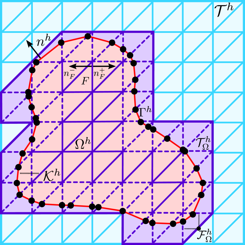
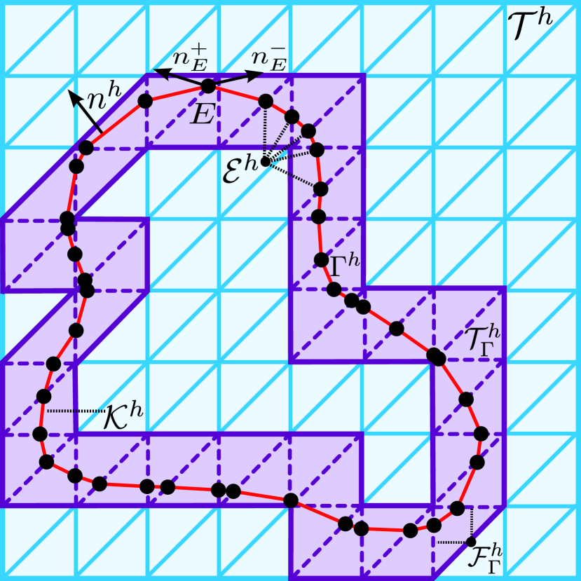
Figure 1: Computational domains for the bulk-surface problem. (Left) Active mesh used to define the approximation space for the bulk solution. Faces on which ghost penalty stabilization are defined are plotted as dashed faces. (Right) Corresponding computational domain set-up for the discretization of the surface.

3.2 The cut discontinuous Galerkin method

We start with defining the discrete counterparts of the function spaces $V_{\Omega}$ and $V_{\Gamma}$ to be the broken polynomial spaces consisting of piecewise linear, but not necessarily globally continuous functions defined on the respective active meshes:

$$V_{\Omega}^{h}=\bigoplus_{T\in\mathcal{T}_{\Omega}^{h}}P_{1}(T),\quad V_{\Gamma}^{h}=\bigoplus_{T\in\mathcal{T}_{\Gamma}^{h}}P_{1}(T),\quad V^{h}=V_{\Omega}^{h}\times V_{\Gamma}^{h}.$$ (23)

For the formulation of the cut discontinuous Galerkin method, we also need the notation of average and fluxes of piecewise defined functions. More precisely, assume that $\sigma$ and $w$ are, possibly vector-valued, elementwise defined functions on $\mathcal{T}^{h}$ which are smooth enough to admit a two-valued trace on all faces. Then the standard and face normal weighted average fluxes are given by

$$\langle{\sigma}\rangle|_{F} =\dfrac{1}{2}(\sigma_{F}^{+}+\sigma_{F}^{-}),$$ (24)

$$\langle{n_{F}\cdot\sigma}\rangle|_{F} =\dfrac{1}{2}n^{+}_{F}\cdot(\sigma_{F}^{+}+\sigma_{F}^{-})=\dfrac{1}{2}(n^{+}_{F}\cdot\sigma_{F}^{+}-n^{-}_{F}\cdot\sigma_{F}^{-}),$$ (25)

while the jump across an interior face $F\in\mathcal{F}^{h}$ is defined by

$$[w]|_{F} =w_{F}^{+}-w_{F}^{-},$$ (26)

with $w(x)^{\pm}=\lim_{t\rightarrow 0^{+}}w(x-tn_{F}^{\pm})$. In the case of vector-valued functions, the jump is taken componentwise. As the co-normal vectors $n_{E}^{\pm}$ are generally not collinear, the standard and co-normal weighted average fluxes for a piecewise discontinuous, possibly vector-valued function $\sigma$ on $\mathcal{K}^{h}$ is defined by

$$\langle{\sigma}\rangle|_{E} =\dfrac{1}{2}(\sigma_{E}^{+}+\sigma_{E}^{-}),$$ (27)

$$\langle{n_{E}\cdot\sigma}\rangle|_{E} =\dfrac{1}{2}(n^{+}_{E}\cdot\sigma_{E}^{+}-n^{-}_{E}\cdot\sigma_{E}^{-}),$$ (28)

respectively. Similarly, the jump across an interior face $E\in\mathcal{E}^{h}$ is given by

$$[w]|_{E} =w_{E}^{+}-w_{E}^{-}.$$ (29)

We are now ready to define the discrete, discontinuous Galerkin counterparts of the bilinear forms (7), (8), and (9) and set

$$a_{\Omega}^{h}(v_{\Omega},w_{\Omega}) =(\nabla v_{\Omega},\nabla w_{\Omega})_{\mathcal{T}_{\Omega}^{h}\cap\Omega^{h}}+(v_{\Omega},w_{\Omega})_{\mathcal{T}_{\Omega}^{h}\cap\Omega^{h}}+\gamma_{\Omega}(h^{-1}[v_{\Omega}],[w_{\Omega}])_{\mathcal{F}_{\Omega}^{h}}$$

$$\qquad-(\langle{n_{F}\cdot\nabla v_{\Omega}}\rangle,[w_{\Omega}])_{\mathcal{F}_{\Omega}^{h}\cap\Omega^{h}}-([v_{\Omega}],\langle{n_{F}\cdot\nabla w_{\Omega}}\rangle)_{\mathcal{F}_{\Omega}^{h}\cap\Omega^{h}},$$ (30)

$$a_{\Gamma}^{h}(v_{\Gamma},w_{\Gamma}) =(\nabla_{\Gamma^{h}}v_{\Gamma},\nabla_{\Gamma^{h}}w_{\Gamma})_{\mathcal{K}^{h}}+(v_{\Gamma},w_{\Gamma})_{\mathcal{T}_{\Gamma}^{h}\cap\Gamma^{h}}+\gamma_{\Gamma}(h^{-1}[v_{\Gamma}],[w_{\Gamma}])_{\mathcal{E}^{h}}$$

$$\qquad-(\langle{n_{E}\cdot\nabla v_{\Gamma}}\rangle,[w_{\Gamma}])_{\mathcal{E}^{h}}-([v_{\Gamma}],\langle{n_{E}\cdot\nabla w_{\Gamma}}\rangle)_{\mathcal{E}^{h}},$$ (31)

$$a_{\Omega\Gamma}^{h}(v,w) =(c_{\Omega}v_{\Omega}-c_{\Gamma}v_{\Gamma},c_{\Omega}w_{\Omega}-c_{\Gamma}w_{\Gamma})_{\Gamma^{h}},$$ (32)

$$a^{h}(v,w) =c_{\Omega}a_{\Omega}^{h}(v_{\Omega},w_{\Omega})+c_{\Gamma}a_{\Gamma}^{h}(v_{\Gamma},w_{\Gamma})+a^{h}_{\Omega\Gamma}(v,w).$$ (33)

Similarly, the relevant discrete linear forms are given by

$$l_{\Omega}^{h}(v_{\Omega}) =(f_{\Omega},v_{\Omega})_{\Omega^{h}},$$ (34)

$$l_{\Gamma}^{h}(v_{\Gamma}) =(f_{\Gamma}^{e},v_{\Gamma})_{\Gamma^{h}},$$ (35)

$$l^{h}(v) =c_{\Omega}l_{\Omega}^{h}(v_{\Omega})+c_{\Gamma}l_{\Gamma}^{h}(v_{\Gamma}).$$ (36)

Here, $f_{\Gamma}^{e}$ denotes the extension of $f_{\Gamma}$ to the tubular neighborhood $U_{\delta}(\Gamma)$ using the closest point projection by requiring that $f_{\Gamma}^{e}(x)=f_{\Gamma}(p(x))$. Finally, appropriate ghost-penalties for the bulk and surface part are defined by

$$j_{\Omega}^{h}(v_{\Omega},w_{\Omega}) =\mu_{\Omega}h^{-1}([v_{\Omega}],[w_{\Omega}])_{\mathcal{F}_{\Omega,g}^{h}}+\tau_{\Omega}h(n_{F}\cdot[\nabla v_{\Omega}],n_{F}\cdot[\nabla w_{\Omega}])_{\mathcal{F}_{\Omega,g}^{h}}$$ (37)

$$j_{\Gamma}^{h}(v_{\Gamma},w_{\Gamma}) =\mu_{\Gamma}h^{-2}([v_{\Gamma}],[w_{\Gamma}])_{\mathcal{F}_{\Gamma}^{h}}+\tau_{\Gamma}(n_{F}\cdot[\nabla v_{\Gamma}],n_{F}\cdot[\nabla w_{\Gamma}])_{\mathcal{F}_{\Gamma}^{h}}$$ (38)

$$j^{h}(v,w) =c_{\Omega}j_{\Omega}^{h}(v_{\Omega},w_{\Omega})+c_{\Gamma}j_{\Gamma}^{h}(v_{\Gamma},w_{\Gamma})$$ (39)

where $\mu_{\Omega},\mu_{\Gamma},\tau_{\Omega},\tau_{\Gamma}$ are positive parameters. To ease the notation, we also define the ghost penalty enhanced bulk and surface bilinear forms

$$A_{U}^{h}(v_{U},w_{U})=a_{U}^{h}(v_{U},w_{U})+j_{U}^{h}(v_{U},w_{U}),\quad U\in\{\Omega,\Gamma\}.$$ (40)

Now the cut discontinuous Galerkin method for the bulk-surface problem is to seek $u^{h}=(u_{\Omega}^{h},u_{\Gamma}^{h})\in V^{h}=V_{\Omega}^{h}\times V_{\Gamma}^{h}$ such that $\forall\,v\in V^{h}$

$$A^{h}(u^{h},v)\coloneqq a^{h}(u^{h},v)+j^{h}(u^{h},v)=l^{h}(v).$$ (41)

Remark 1

The defined ghost penalties are crucial to devise a geometrically robust, well-conditioned and optimally convergent discretization method, irrespective of the particular cut configuration. We note that in general, the unstabilized cutDGM suffers from three drawbacks. First, certain inverse inequalities fundamental for the analysis of DGMs do not hold any more when only the physical, cut part of the background mesh is considered. Second, cut configurations with very small cut parts can lead to an almost vanishing contribution of certain degree of freedoms in the system matrix. Third, the restriction of discontinuous finite element functions from the active mesh $\mathcal{T}_{\Gamma}^{h}$ to the surface $\Gamma^{h}$ results in a highly linear dependent set of functions, and thus purely surface-based “norms”are not capable of distinguishing them, which also leads to an ill-conditioned system matrix.

4 Stability properties

In this section, we investigate the stability properties of the proposed cutDGM for the coupled bulk-surface problem. In particular, we show that the ghost-penalty enhanced discrete form $A_{h}$ is coercive with respect to a natural discrete energy-norm and that the condition number of the resulting system matrix scales as $\mathcal{O}(h^{-2})$, irrespective of the position of $\Omega^{h}$ relative to the background mesh $\mathcal{T}^{h}$.

4.1 Norms and coercivity

A natural discrete energy-norm for the forthcoming stability analysis is given by combining the individual discrete energy norms for the bulk and surface parts,

$$|\mspace{-1.0mu}|\mspace{-1.0mu}|v_{\Omega}|\mspace{-1.0mu}|\mspace{-1.0mu}|_{h,\Omega}^{2} =\|\nabla v_{\Omega}\|^{2}_{\Omega^{h}}+\|v_{\Omega}\|^{2}_{\Omega^{h}}+\|h^{-\frac{1}{2}}[v_{\Omega}]\|^{2}_{\mathcal{F}^{h}}+j_{\Omega}^{h}(v_{\Omega},v_{\Omega}),$$ (42)

$$|\mspace{-1.0mu}|\mspace{-1.0mu}|v_{\Gamma}|\mspace{-1.0mu}|\mspace{-1.0mu}|_{h,\Gamma}^{2} =\|\nabla_{\Gamma^{h}}v_{\Gamma}\|^{2}_{\Gamma^{h}}+\|v_{\Gamma}\|^{2}_{\Gamma^{h}}+\|h^{-\frac{1}{2}}[v_{\Gamma}]\|^{2}_{\mathcal{E}^{h}}+j_{\Gamma}^{h}(v_{\Gamma},v_{\Gamma}),$$ (43)

with the semi-norm induced by the coupling bilinear $$a^{h}_{\Omega\Gamma}$$ to define

$$|\mspace{-1.0mu}|\mspace{-1.0mu}|v|\mspace{-1.0mu}|\mspace{-1.0mu}|_{h}^{2} =c_{\Omega}|\mspace{-1.0mu}|\mspace{-1.0mu}|v_{\Omega}|\mspace{-1.0mu}|\mspace{-1.0mu}|_{h,\Omega}^{2}+c_{\Gamma}|\mspace{-1.0mu}|\mspace{-1.0mu}|v_{\Gamma}|\mspace{-1.0mu}|\mspace{-1.0mu}|_{h,\Gamma}^{2}+\|c_{\Omega}v_{\Omega}-c_{\Gamma}v_{\Gamma}\|_{\Gamma^{h}}^{2}.$$ (44)

With these norm definitions, the coercivity of the total bilinear form $A^{h}$ can be easily shown once coercivity properties for the bulk and surface bilinear form are established individually. In other words, we wish to show that

$$|\mspace{-1.0mu}|\mspace{-1.0mu}|v_{\Omega}|\mspace{-1.0mu}|\mspace{-1.0mu}|_{h,\Omega}^{2} \lesssim A_{\Omega}(v_{\Omega},v_{\Omega}) \quad\forall\,v_{\Omega}\in V_{\Omega}^{h},$$ (45)

$$|\mspace{-1.0mu}|\mspace{-1.0mu}|v_{\Gamma}|\mspace{-1.0mu}|\mspace{-1.0mu}|_{h,\Gamma}^{2} \lesssim A_{\Gamma}(v_{\Gamma},v_{\Gamma}) \quad\forall\,v_{\Gamma}\in V_{\Gamma}^{h},$$ (46)

which together with the simple observation that

$$A^{h}(v,v) =A_{\Omega}^{h}(v_{\Omega},v_{\Omega})+A_{\Gamma}^{h}(v_{\Gamma},v_{\Gamma})+a_{\Omega\Gamma}^{h}(v,v)$$ (47)

$$\gtrsim|\mspace{-1.0mu}|\mspace{-1.0mu}|v_{\Omega}|\mspace{-1.0mu}|\mspace{-1.0mu}|_{h,\Omega}^{2}+|\mspace{-1.0mu}|\mspace{-1.0mu}|v_{\Gamma}|\mspace{-1.0mu}|\mspace{-1.0mu}|_{h,\Gamma}^{2}+\|c_{\Omega}v_{\Omega}-c_{\Gamma}v_{\Gamma}\|_{\Gamma^{h}}^{2},$$ (48)

leads us to the following proposition.

Proposition 1

The discrete bilinear form $A^{h}$ is coercive with respect to the discrete energy norm (44):

$$|\mspace{-1.0mu}|\mspace{-1.0mu}|v|\mspace{-1.0mu}|\mspace{-1.0mu}|_{h}^{2} \lesssim A^{h}(v,v),\quad\forall\,v\in V^{h}.$$ (49)

The following two subsection are thus devoted to prove that the estimates (45) and (46) hold.

4.2 Coercivity of the discrete bulk form $A_{\Omega}^{h}$

A standard ingredient in the numerical analysis of discontinuous Galerkin methods is the inverse inequality

$$\|n_{F}\cdot\nabla v\|_{F}\leqslant C_{I}h_{T}^{-\frac{1}{2}}\|\nabla v\|_{T},$$ (50)

which holds for discrete functions $v\in P_{1}(T)$. Here, the face $F$ is part of the element boundary $\partial T$ and the inverse constant $C_{I}=C_{I}(\tfrac{|F|}{|T|})$ depends on the ratio of the face area $|F|$ and element volume $|T|$, and thus ultimately on the shape regularity of $\mathcal{T}^{h}$. Unfortunately, a corresponding inverse inequality of the form

$$\|n_{F}\cdot\nabla v\|_{F\cap\Omega^{h}}\leqslant C_{I}h_{T}^{-\frac{1}{2}}\|\nabla v\|_{T\cap\Omega^{h}}$$ (51)

does not hold as the ratio $\tfrac{|F|}{|T|}$ can become arbitrarily large, depending on the cut configuration. As a partial replacement, one might be tempted to use the simple estimate

$$\|n_{F}\cdot\nabla v\|_{F\cap\Omega^{h}}\leqslant\|n_{F}\cdot\nabla v\|_{F}\leqslant C_{I}h_{T}^{-\frac{1}{2}}\|\nabla v\|_{T}$$ (52)

instead. To fully exploit this idea, it is necessary to extend the control of the $\|\nabla v\|^{2}_{\Omega^{h}}$ part in natural energy norm associated with $a_{\Omega}^{h}$ from the physical domain $\Omega^{h}$ to the entire active mesh $\mathcal{T}_{\Omega}^{h}$. This is precisely the role of the ghost-penalty term $j_{\Omega}^{h}$:

Lemma 1

For $v\in V_{\Omega}^{h}$ it holds that

$$\|\nabla v\|_{\mathcal{T}_{\Omega}^{h}}^{2}\lesssim\|\nabla v\|_{\Omega^{h}}^{2}+j_{\Omega}^{h}(v,v)\lesssim\|\nabla v\|_{\mathcal{T}_{\Omega}^{h}}^{2},$$ (53)

and consequently, using (52)

$$\|h^{\frac{1}{2}}n_{F}\cdot\nabla v\|_{\mathcal{F}_{\Omega}^{h}\cap\Omega^{h}}^{2}\lesssim\|\nabla v\|_{\Omega^{h}}^{2}+j_{\Omega}^{h}(v,v),$$ (54)

with the hidden constant depending only in the shape-regularity of $\mathcal{T}^{h}$.

Proof

For a detailed proof, we refer to Burman and Hansbo (2012); Massing (2012); Massing et al. (2014).

Thanks to the ghost penalty Lemma 1, we can establish the coercivity of $A_{\Omega}^{h}$ by simply following the standard arguments in the classical proof for symmetric interior penalty methods.

Proposition 2

The discrete bulk form $A_{\Omega}^{h}$ is coercive with respect to the discrete energy norm $|\mspace{-1.0mu}|\mspace{-1.0mu}|\cdot|\mspace{-1.0mu}|\mspace{-1.0mu}|_{h,\Omega}$; that is,

$$|\mspace{-1.0mu}|\mspace{-1.0mu}|v|\mspace{-1.0mu}|\mspace{-1.0mu}|_{h,\Omega}^{2}\lesssim A_{\Omega}^{h}(v,v),\quad\forall\,v\in V_{\Omega}^{h},$$ (55)

Proof

We follow closely the standard arguments. Setting $w_{\Omega}=v_{\Omega}$ in (30) and combining the ghost-penalty Lemma 1 and a $\epsilon$-Cauchy-Schwarz inequality of the form $2ab\leqslant\epsilon a^{2}+\epsilon^{-1}b^{2}$ with an inverse estimate yields

$$A_{\Omega}^{h}(v,v) =\|\nabla v\|_{\Omega^{h}}^{2}-2(\langle{n_{F}\cdot\nabla v}\rangle,[v])_{\mathcal{F}_{\Omega}^{h}\cap\Omega^{h}}+\gamma_{\Omega}\|h^{-\frac{1}{2}}[v]\|_{\mathcal{F}_{\Omega}^{h}}^{2}$$ (56)

$$\quad+j_{\Omega}^{h}(v,v)+\|v\|_{\Omega^{h}}^{2}$$ (57)

$$\gtrsim\|\nabla v\|_{\mathcal{T}_{\Omega}^{h}}^{2}-\epsilon\|h^{\frac{1}{2}}\langle{n_{F}\cdot\nabla v_{\Gamma}}\rangle\|_{\mathcal{F}_{\Omega}^{h}}^{2}-\epsilon^{-1}\|h^{-\frac{1}{2}}[v]\|_{\mathcal{F}_{\Omega}^{h}}\|^{2}$$ (58)

$$\quad+\gamma_{\Omega}\|h^{-\frac{1}{2}}[v]\|_{\mathcal{F}_{\Omega}^{h}}^{2}+\frac{1}{2}j_{\Omega}^{h}(v,v)+\|v\|_{\Omega^{h}}^{2}$$ (59)

$$\gtrsim(1-\epsilon C_{I})\|\nabla v\|_{\mathcal{T}_{\Omega}^{h}}^{2}$$ (60)

$$\quad+(\gamma_{\Omega}-\epsilon^{-1})\|h^{-\frac{1}{2}}[v]\|_{\mathcal{F}_{\Omega}^{h}}^{2}+\frac{1}{2}j_{\Omega}^{h}(v,v)+\|v\|_{\Omega^{h}}^{2}\gtrsim|\mspace{-1.0mu}|\mspace{-1.0mu}|v|\mspace{-1.0mu}|\mspace{-1.0mu}|_{h,\Omega}^{2}$$ (61)

if we chose $0<\epsilon\lesssim 1/(2C_{I})$ small enough and $\gamma_{\Omega}>\epsilon^{-1}$.

4.3 Coercivity of the discrete surface form $A_{\Gamma}^{h}$

Next, we turn to the stability properties of the discrete surface form $A_{\Gamma}^{h}$. First observe that the unstabilized DG energy “norm”

$$|\mspace{-1.0mu}|\mspace{-1.0mu}|v|\mspace{-1.0mu}|\mspace{-1.0mu}|_{\Gamma}^{2}\coloneqq\|\nabla_{\Gamma^{h}}v\|_{{\Gamma^{h}}}^{2}+\|v\|_{{\Gamma^{h}}}^{2}+\|h^{-\frac{1}{2}}[v]\|_{\mathcal{E}^{h}}^{2}$$ (62)

does not define an actual norm on $V_{\Gamma}^{h}$. For instance, the piecewise linear and continuous approximation $\rho^{h}$ of the distance function $\rho$ vanishes on ${\Gamma^{h}}$. It was shown in Burman et al. (2016) that a proper norm can obtained if the ghost penalty term $j_{\Gamma}^{h}$ was added, resulting in our norm definition (43). More, precisely, the following discrete Poincaré inequality was established.

Lemma 2

Let $h\in(0,h_{0}]$ with $h_{0}$ small enough. Then the following estimate holds:

$$h^{-1}\|v-\lambda_{\Gamma^{h}}(v)\|^{2}_{\mathcal{T}^{h}}\lesssim\|\nabla_{\Gamma^{h}}v\|^{2}_{\Gamma^{h}}+j_{\Gamma}^{h}(v,v)\quad\forall v\in V^{h},$$ (63)

where $\lambda_{\Gamma^{h}}(v)=\tfrac{1}{|{\Gamma^{h}}|}\int_{{\Gamma^{h}}}v\,\mathrm{d}\Gamma^{h}$ is the mean value of $v$ on ${\Gamma^{h}}$.

To prove that $A_{\Gamma}^{h}$ is in fact coercive with respect to a properly defined discrete energy norm, we need to borrow one more result from Burman et al. (2016) which allows us to control the co-normal flux $n_{E}\cdot\nabla_{\Gamma^{h}}v$ for $v\in V_{\Gamma}^{h}$.

Lemma 3

The following estimate holds

$$h\|\nabla_{\Gamma^{h}}v\|^{2}_{\partial\mathcal{K}_{h}}\lesssim\|\nabla_{\Gamma^{h}}v\|^{2}_{\Gamma^{h}}+j_{\Gamma}^{h}(v,v),$$ (64)

for $0<h\leq h_{0}$ with $h_{0}$ small enough.

Now simply replacing the crucial normal-flux estimate (54) with co-normal flux estimate from the previous Lemma (3), the proof of Lemma 2 literally transfers to the surface case, and thus we have established the following result.

Proposition 3

The discrete surface form $A_{\Gamma}^{h}$ is coercive with respect to the discrete energy norm $|\mspace{-1.0mu}|\mspace{-1.0mu}|\cdot|\mspace{-1.0mu}|\mspace{-1.0mu}|_{h,\Gamma}$:

$$|\mspace{-1.0mu}|\mspace{-1.0mu}|v|\mspace{-1.0mu}|\mspace{-1.0mu}|_{h,\Gamma}^{2} \lesssim A_{\Gamma}^{h}(v,v),\quad\forall\,v\in V_{\Gamma}^{h}.$$ (65)

4.4 Condition number estimates

Following closely the presentation in Burman et al. (2016), we now show that the condition number of the system matrix associated with a properly rescaled version of the bilinear form (11) can be bounded by $O(h^{-2})$ independently of the position of the bulk domain $\Omega$ relative to the background mesh $\mathcal{T}_{h}$. Let $\{\phi_{\Omega,i}\}_{i=1}^{N_{\Omega}}$ and $\{\phi_{\Gamma,i}\}_{i=1}^{N_{\Gamma}}$ be the standard piecewise linear basis functions associated with $\mathcal{T}_{\Omega}^{h}$ and $\mathcal{T}_{\Gamma}^{h}$, respectively. Thus

$$v^{h}=(v_{\Gamma}^{h},v_{\Omega}^{h})=\Bigl{(}\sum_{i=1}^{N_{\Omega}}V_{\Omega,i}\phi_{\Omega,i},\sum_{i=1}^{N_{\Gamma}}V_{\Gamma,i}\phi_{\Gamma,i}\Bigr{)}$$ (66)

for $v^{h}\in V^{h}$ and expansion coefficients $V=\bigl{(}\{V_{\Omega,i}\}_{i=1}^{N_{\Omega}},\{V_{\Gamma,i}\}_{i=1}^{N_{\Gamma}}\bigl{)}\in\mathbb{R}^{N_{\Omega}}\times\mathbb{R}^{N_{\Gamma}}=\mathbb{R}^{N}$ with $N=N_{\Omega}+N_{\Gamma}$. It is well-known that for any quasi-uniform mesh $\mathcal{T}^{h}$ consisting of $d$-dimensional simplices, the continuous $\|\cdot\|_{L^{2}(\mathcal{T}^{h})}$- norm of a finite element function $v\in\mathcal{V}^{h}=\operatorname{span}(\{\phi_{i}\}_{i=1}^{M})$ is related to the discrete $\|\cdot\|_{l^{2}(\mathbb{R}^{M})}$ of its corresponding coefficient vector $V$ via

$$h^{d/2}\|V\|_{\mathbb{R}^{M}}\lesssim\|v_{h}\|_{L^{2}(\mathcal{T}^{h})}\lesssim h^{d/2}\|V\|_{\mathbb{R}^{M}}.$$ (67)

Note that due to the different Hausdorff dimensions of the surface and bulk domain, the discrete norms and forms for each domain scale differently with respect to the mesh size $h$. For instance, we have clearly the Poincaré-type estimate

$$\|v_{\Omega}\|_{\mathcal{T}_{\Omega}^{h}}\lesssim|\mspace{-1.0mu}|\mspace{-1.0mu}|v_{\Omega}|\mspace{-1.0mu}|\mspace{-1.0mu}|_{h,\Omega}\quad\forall\,v_{\Omega}\in V_{\Omega}^{h},$$ (68)

while for the surface problem, Lemma 2 shows that we have

$$\|v_{\Gamma}\|_{\mathcal{T}_{\Gamma}^{h}}\lesssim|\mspace{-1.0mu}|\mspace{-1.0mu}|h^{\frac{1}{2}}v_{\Gamma}|\mspace{-1.0mu}|\mspace{-1.0mu}|_{h,\Gamma}\quad\forall\,v_{\Gamma}\in V_{\Gamma}^{h}.$$ (69)

Thus in order to pass back and forth between discrete $l^{2}$ and continuous, similarly scaled $L^{2}$ norms on the surface and in the bulk domain, it is natural to rescale the discrete surface functions. More precisely, the system matrix $\mathcal{A}$ we will consider is given by the relation

$$(\mathcal{A}V,W)_{\mathbb{R}^{N}}=\widetilde{A}_{h}(v_{h},w_{h})\coloneqq{A}_{h}(v_{h},h^{\frac{1}{2}}w_{h})\quad\forall\,v_{h},w_{h}\in V_{h}.$$ (70)

The system matrix $\mathcal{A}$ is a bijective linear mapping $\mathcal{A}:\mathbb{R}^{N}\to\mathbb{R}^{N}$. The operator norm and condition number of the matrix $\mathcal{A}$ are then defined by

$$\|\mathcal{A}\|_{\mathbb{R}^{N}}=\sup_{V\in\widehat{\mathbb{R}}^{N}\setminus 0}\dfrac{\|\mathcal{A}V\|_{\mathbb{R}^{N}}}{\|V\|_{N}}\quad\text{and}\quad\kappa(\mathcal{A})=\|\mathcal{A}\|_{\mathbb{R}^{N}}\|\mathcal{A}^{-1}\|_{\mathbb{R}^{N}}$$ (71)

respectively. Following the approach in Ern and Guermond (2006), a bound for the condition number can be derived by combining (67) with suitable Poincaré-type estimates and inverse estimates relating the $L^{2}$ norm to the discrete energy norms. An immediate consequence of the discrete Poincaré estimates for the discrete bulk and surface energy norms given by (68) and (69), respectively, is the following Poincaré estimate for the total discrete energy norm:

Lemma 4

For $(v_{\Omega},v_{\Gamma})\in V^{h}=V_{\Omega}^{h}\times V_{\Gamma}^{h}$ it holds

$$\|(v_{\Omega},v_{\Gamma})\|_{\mathcal{T}_{\Omega}^{h}\times\mathcal{T}_{\Gamma}^{h}}\lesssim|\mspace{-1.0mu}|\mspace{-1.0mu}|(v_{\Omega},h^{\frac{1}{2}}v_{\Gamma})|\mspace{-1.0mu}|\mspace{-1.0mu}|_{h}.$$ (72)

Before we turn to formulate and prove a suitable inverse inequality for the total discrete energy norm, we briefly recall that we have the following inverse inequalities:

$$\|\nabla v\|_{T} \lesssim h^{-1}\|v\|_{T}, \quad\forall\,v\in V_{\Omega}^{h},$$ (73)

$$\|v\|_{F} \lesssim h^{-\frac{1}{2}}\|v\|_{T}, \quad\forall\,v\in V_{\Omega}^{h},$$ (74)

$$\|v\|_{\Gamma^{h}\cap T} \lesssim h^{-\frac{1}{2}}\|v\|_{T}, \quad\forall\,v\in V_{\Gamma}^{h}.$$ (75)

While the first two are standard, the third one is less known and can be found in, e.g., Burman et al. (2015c, 2016, 2016, 2016). Now it is easy to show the following inverse inequality.

Lemma 5

For $(v_{\Omega},v_{\Gamma})\in V^{h}=V_{\Omega}^{h}\times V_{\Gamma}^{h}$ it holds

$$|\mspace{-1.0mu}|\mspace{-1.0mu}|(v_{\Omega},h^{\frac{1}{2}}v_{\Gamma})|\mspace{-1.0mu}|\mspace{-1.0mu}|_{h}\lesssim h^{-1}\|(v_{\Omega},v_{\Gamma})\|_{\mathcal{T}_{\Omega}^{h}\times\mathcal{T}_{\Gamma}^{h}}.$$ (76)

Proof

Recalling the definition of $|\mspace{-1.0mu}|\mspace{-1.0mu}|\cdot|\mspace{-1.0mu}|\mspace{-1.0mu}|_{h}$,

$$|\mspace{-1.0mu}|\mspace{-1.0mu}|(v_{\Omega},h^{\frac{1}{2}}v_{\Gamma})|\mspace{-1.0mu}|\mspace{-1.0mu}|_{h}^{2} =|\mspace{-1.0mu}|\mspace{-1.0mu}|v_{\Omega}|\mspace{-1.0mu}|\mspace{-1.0mu}|_{h,\Omega}^{2}+|\mspace{-1.0mu}|\mspace{-1.0mu}|h^{\frac{1}{2}}v_{\Gamma}|\mspace{-1.0mu}|\mspace{-1.0mu}|_{h,\Gamma}^{2}+\|c_{\Omega}v_{\Omega}-h^{\frac{1}{2}}c_{\Gamma}v_{\Gamma}\|_{\Gamma^{h}}^{2}$$ (77)

$$=I+II+III,$$ (78)

it is enough to consider the last two terms, as term $I$ can be treated similar to $II$. We start with the contributions of $II$ which are not related to $j_{\Gamma}^{h}$ and after successively applying variants of the inverse estimates type (73), (75), we get

$$\|h^{\frac{1}{2}}\nabla_{\Gamma^{h}}v_{\Gamma}\|_{\Gamma^{h}} \lesssim\|\nabla v_{\Gamma}\|_{\mathcal{T}_{\Gamma}^{h}}\lesssim h^{-1}\|v_{\Gamma}\|_{\mathcal{T}_{\Gamma}^{h}},$$ (79)

$$\|h^{\frac{1}{2}}v_{\Gamma}\|_{\Gamma^{h}} \lesssim\|v_{\Gamma}\|_{\mathcal{T}_{\Gamma}^{h}},$$ (80)

$$\|h^{-\frac{1}{2}}[h^{\frac{1}{2}}v_{\Gamma}]\|_{\mathcal{E}^{h}\cap T} \lesssim h^{-1}\|v_{\Gamma}\|_{\mathcal{T}_{\Gamma}^{h}}.$$ (81)

Turning to the contribution from $j_{\Gamma}^{h}$, we see that

$$j_{\Gamma}^{h}(h^{\frac{1}{2}}v_{\Gamma},h^{\frac{1}{2}}v_{\Gamma})^{\frac{1}{2}} \lesssim h^{-1}\|[h^{\frac{1}{2}}v_{\Gamma}]\|_{\mathcal{F}_{\Gamma}^{h}}+\|[h^{\frac{1}{2}}n_{F}\cdot\nabla v_{\Gamma}]\|_{\mathcal{F}_{\Gamma}^{h}}\lesssim h^{-1}\|v_{\Gamma}\|_{\mathcal{T}_{\Gamma}^{h}}.$$ (82)

Finally, we conclude the proof by estimating the remaining term $III$ as follows,

$$III\lesssim\|c_{\Omega}v_{\Omega}\|_{\Gamma^{h}}+\|h^{\frac{1}{2}}c_{\Gamma}v_{\Gamma}\|_{\Gamma^{h}}\lesssim h^{-\frac{1}{2}}\|c_{\Omega}v_{\Omega}\|_{\mathcal{T}_{\Omega}^{h}}+\|c_{\Gamma}v_{\Gamma}\|_{\mathcal{T}_{\Gamma}^{h}}.$$ (83)

Theorem 4.1

The condition number of the stiffness matrix satisfies the estimate

$$\kappa(\mathcal{A})\lesssim h^{-2},$$ (84)

where the hidden constant depends only on the quasi-uniformity of the background mesh $\mathcal{T}^{h}$ and the chosen stability parameters.

Proof

We need to bound $\|\mathcal{A}\|_{\mathbb{R}^{N}}$ and $\|\mathcal{A}^{-1}\|_{\mathbb{R}^{N}}$. To derive a bound for $\|\mathcal{A}\|_{\mathbb{R}^{N}}$, we first use the inverse estimate (76) and equivalence (67) to find that $\forall\,w\in V^{h}$,

$$|\mspace{-1.0mu}|\mspace{-1.0mu}|(w_{\Omega},h^{\frac{1}{2}}w_{\Gamma})|\mspace{-1.0mu}|\mspace{-1.0mu}|_{h}\lesssim h^{-1}\|(w_{\Omega},w_{\Gamma})\|_{\mathcal{T}_{\Omega}^{h}\times\mathcal{T}_{\Gamma}^{h}}\lesssim h^{(d-2)/2}\|W\|_{\mathbb{R}^{N}}.$$ (85)

Then

$$\|\mathcal{A}V\|_{\mathbb{R}^{N}} =\sup_{W\in\mathbb{R}^{N}}\frac{(\mathcal{A}V,W)_{\mathbb{R}^{N}}}{\|W\|_{\mathbb{R}^{d}}}=\sup_{w\in V_{h}}\frac{\widetilde{A}^{h}(v,w)}{|\mspace{-1.0mu}|\mspace{-1.0mu}|(w_{\Omega},h^{\frac{1}{2}}w_{\Gamma})|\mspace{-1.0mu}|\mspace{-1.0mu}|_{h}}\frac{|\mspace{-1.0mu}|\mspace{-1.0mu}|(w_{\Omega},h^{\frac{1}{2}}w_{\Gamma})|\mspace{-1.0mu}|\mspace{-1.0mu}|_{h}}{\|W\|_{\mathbb{R}^{N}}}$$ (86)

$$\lesssim h^{(d-2)/2}|\mspace{-1.0mu}|\mspace{-1.0mu}|(v_{\Omega},h^{\frac{1}{2}}v_{\Gamma})|\mspace{-1.0mu}|\mspace{-1.0mu}|_{h}\lesssim h^{d-2}\|V\|_{N},$$ (87)

and thus by the definition of the operator norm, $\|\mathcal{A}\|_{\mathbb{R}^{N}}\lesssim h^{d-2}$. Next we turn to the estimate of $\|\mathcal{A}^{-1}\|_{\mathbb{R}^{N}}$. Starting from (67) and combining the Poincaré inequality (72) with the stability estimates (55) and a Cauchy Schwarz inequality, we arrive at the following chain of estimates:

$$\|V\|^{2}_{\mathbb{R}^{N}} \lesssim h^{-d}\|(v_{\Omega},v_{\Gamma})\|^{2}_{\Omega^{h}\times\Gamma^{h}}\lesssim h^{-d}|\mspace{-1.0mu}|\mspace{-1.0mu}|(v_{\Omega},h^{\frac{1}{2}}v_{\Gamma})|\mspace{-1.0mu}|\mspace{-1.0mu}|_{h}^{2}$$ (88)

$$\lesssim h^{-d}\widetilde{A}_{h}(v,v)=h^{-d}(V,\mathcal{A}V)_{\mathbb{R}^{N}}\lesssim h^{-d}\|V\|_{\mathbb{R}^{N}}\|\mathcal{A}V\|_{\mathbb{R}^{N}},$$ (89)

and hence $\|V\|_{\mathbb{R}^{N}}\lesssim h^{-d}\|\mathcal{A}V\|_{\mathbb{R}^{N}}$. Now setting $V=\mathcal{A}^{-1}W$ we conclude that $\|\mathcal{A}^{-1}\|_{\mathbb{R}^{N}}\lesssim h^{-d}$ and combining the estimates for $\|\mathcal{A}\|_{\mathbb{R}^{N}}$ and $\|\mathcal{A}^{-1}\|_{\mathbb{R}^{N}}$ the theorem follows.

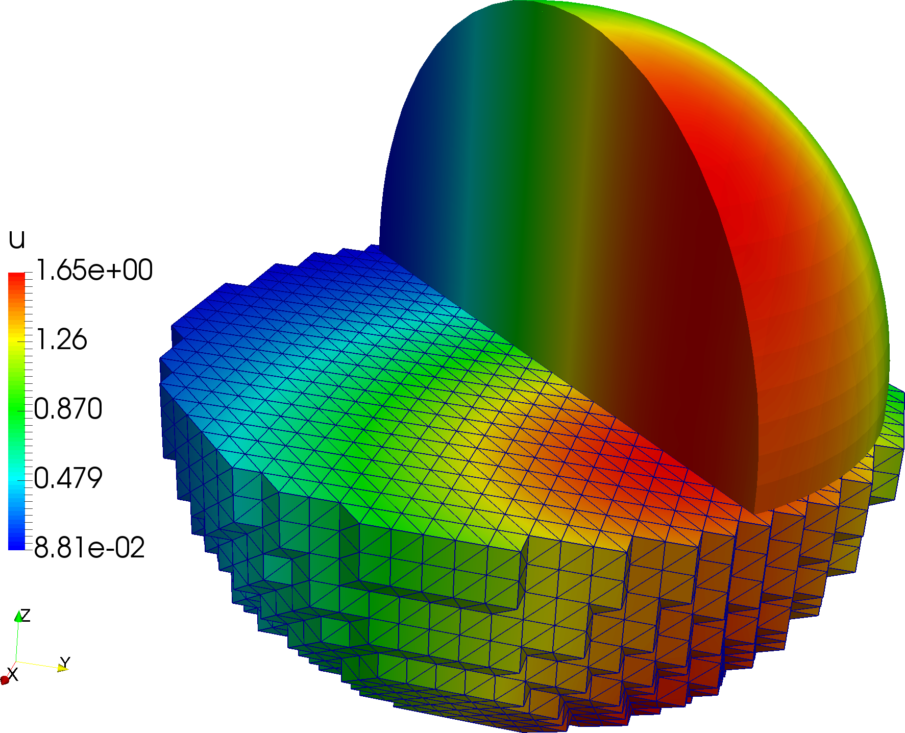
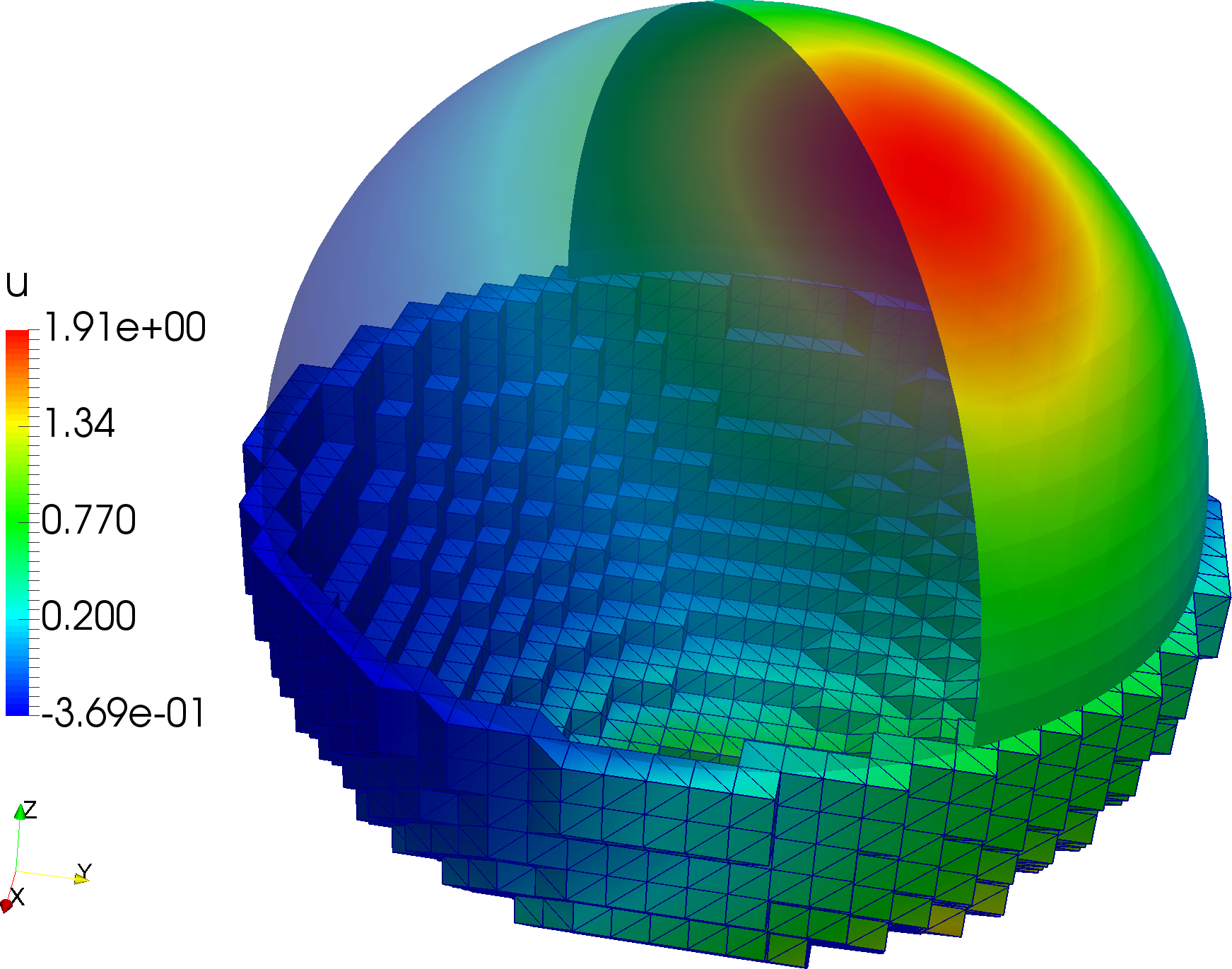
Figure 2: Computed solutions for coupled bulk-surface PDE example. The left plot shows the approximate bulk solution $u_{\Gamma}^{h}$ as computed on the active mesh $\mathcal{T}_{\Omega}^{h}$, together with it restriction to the bulk domain $\Omega^{h}$. The right plot displays the corresponding surface solution $u_{\Gamma}^{h}$.

5 Numerical results

5.1 Convergence rate study

Following the numerical example presented in Elliott and Ranner (2013), we now examine the convergence properties of the presented cutDG method for the bulk-surface problem (2). An analytical reference solution is defined by

$$u_{\Omega}(x,y,z) =c_{\Gamma}e^{-x(x-1)y(y-1)},$$ (90)

$$u_{\Gamma}(x,y,z) =(c_{\Gamma}+x(1-2x)+y(1-2x))e^{-x(x-1)y(y-1)},$$ (91)

with $c_{\Omega}=c_{\Gamma}=1$, the corresponding the right-side $f=(f_{\Omega},f_{\Gamma})$ is computed such that $u=(u_{\Gamma},u_{\Omega})$ satisfies (2a)– (2c). Starting from a structured background mesh $\widetilde{\mathcal{T}}_{0}$ for $\Omega=[-1.1,1.1]^{3}$, a sequence of meshes $\{\mathcal{T}_{k}\}_{k=0}^{5}$ is generated by successively refining $\widetilde{\mathcal{T}}_{0}$ and extracting the relevant active background meshes for the bulk and surface problem as defined by (16)–(17). Based on the manufactured exact solution, the experimental order of convergence (EOC) is calculated by

$$\text{EOC}(k)=\dfrac{\log(E_{k-1}/E_{k})}{\log(2)}$$

with $E_{k}$ denoting the (norm-dependent) error of the numerical solution $u_{k}$ computed at refinement level $k$. In the present convergence study, both $\|\cdot\|_{H^{1}(U)}$ and $\|\cdot\|_{L^{2}(U)}$ for $U\in\{\Omega^{h},\Gamma^{h}\}$ are used to compute $E_{k}$. For the completely stabilized cutDG method with $\gamma_{\Omega}=\gamma_{\Gamma}=50$, $\mu_{\Omega}=\mu_{\Gamma}=50$ and $\tau_{\Omega}=\tau_{\Gamma}=0.01$, the observed EOC reported in Table 1 (top) reveals a first-order and second-order convergence in the $H^{1}$ and $L^{2}$ norm, respectively. Note that for the bulk problem, the standard DG jump penalization term in (30) scaled with $\gamma_{\Omega}$ is similar to the lowest order term in the ghost-penalty (37) scaled with $\mu_{\Omega}$. Deactivating all solely ghost-penalty related stabilization by setting $\tau_{\Omega}=\tau_{\Gamma}=\mu_{\Gamma}=0$ renders the method completely unreliable and thus demonstrates the necessity to stabilize the presented DG method for the bulk-surface problem in the unfitted mesh case.

$k$	$\|e^{h}\|_{H^{1}(\Omega^{h})}$		EOC	$\|e^{k}\|_{L^{2}(\Omega^{h})}$		EOC	$\|e^{k}\|_{H^{1}(\Gamma^{h})}$		EOC	$\|e^{k}\|_{L^{2}(\Gamma^{h})}$		EOC
$0$	$5.28$	$\cdot 10^{-1}$	–	$8.60$	$\cdot 10^{-2}$	–	$2.17$	$\cdot 10^{0}$	–	$2.73$	$\cdot 10^{-1}$	–
$1$	$3.44$	$\cdot 10^{-1}$	$+0.62$	$3.04$	$\cdot 10^{-2}$	$+1.50$	$1.12$	$\cdot 10^{0}$	$+0.96$	$7.38$	$\cdot 10^{-2}$	$+1.89$
$2$	$1.84$	$\cdot 10^{-1}$	$+0.90$	$7.34$	$\cdot 10^{-3}$	$+2.05$	$5.80$	$\cdot 10^{-1}$	$+0.94$	$1.80$	$\cdot 10^{-2}$	$+2.04$
$3$	$9.35$	$\cdot 10^{-2}$	$+0.98$	$1.83$	$\cdot 10^{-3}$	$+2.00$	$2.76$	$\cdot 10^{-1}$	$+1.07$	$4.63$	$\cdot 10^{-3}$	$+1.96$
$4$	$4.71$	$\cdot 10^{-2}$	$+0.99$	$4.66$	$\cdot 10^{-4}$	$+1.98$	$1.39$	$\cdot 10^{-1}$	$+0.99$	$1.07$	$\cdot 10^{-3}$	$+2.12$

$k$	$\|e^{h}\|_{H^{1}(\Omega^{h})}$		EOC	$\|e^{k}\|_{L^{2}(\Omega^{h})}$		EOC	$\|e^{k}\|_{H^{1}(\Gamma^{h})}$		EOC	$\|e^{k}\|_{L^{2}(\Gamma^{h})}$		EOC
$0$	$7.27$	$\cdot 10^{-1}$	–	$1.32$	$\cdot 10^{-1}$	–	$5.38$	$\cdot 10^{0}$	–	$1.16$	$\cdot 10^{0}$	–
$1$	$8.88$	$\cdot 10^{-1}$	$-0.29$	$1.99$	$\cdot 10^{-1}$	$-0.59$	$8.46$	$\cdot 10^{0}$	$-0.65$	$1.82$	$\cdot 10^{0}$	$-0.65$
$2$	$1.14$	$\cdot 10^{0}$	$-0.36$	$2.72$	$\cdot 10^{-1}$	$-0.45$	$1.02$	$\cdot 10^{2}$	$-3.59$	$2.60$	$\cdot 10^{0}$	$-0.51$
$3$	$1.01$	$\cdot 10^{0}$	$+0.17$	$2.51$	$\cdot 10^{-1}$	$+0.11$	$1.87$	$\cdot 10^{1}$	$+2.44$	$2.25$	$\cdot 10^{0}$	$+0.21$

Table 1: Experimental order of convergence for the bulk-surface problem with DG-stabilization parameters $\gamma_{\Omega}=\gamma_{\Gamma}=50$. (Top) Optimal convergence rates are obtained for completely activated ghost-penalties using $\mu_{\Omega}=\mu_{\Gamma}=50$ and $\tau_{\Omega}=\tau_{\Gamma}=0.01$. (Bottom) After deactivation of the ghost penalties by setting $\mu_{\Gamma}=\tau_{\Omega}=\tau_{\Gamma}=0$, the convergence rate deteriorates completely and no clear trend is observable.

5.2 Condition number study

In the second numerical experiment, we study the sensitivity of the condition number of the system matrix defined by (70) with respect to relative positioning of $\Gamma$ within the background mesh $\mathcal{T}_{h}$. Starting from the set-up described in Section 5.1 and choosing refinement level $k=1$, a family of surfaces $\{\Gamma_{\delta}\}_{0\leqslant\delta\leqslant 1}$ is generated by translating the unit-sphere $S^{2}=\{x\in\mathbb{R}^{3}:\|x\|=1\}$ along the diagonal $(h,h,h)$; that is, $\Gamma_{\delta}=S^{2}+\delta_{0}(h,h,h)$ with $\delta\in[0,1]$. Figure 3 illustrates the experimental set-up.

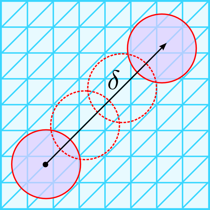
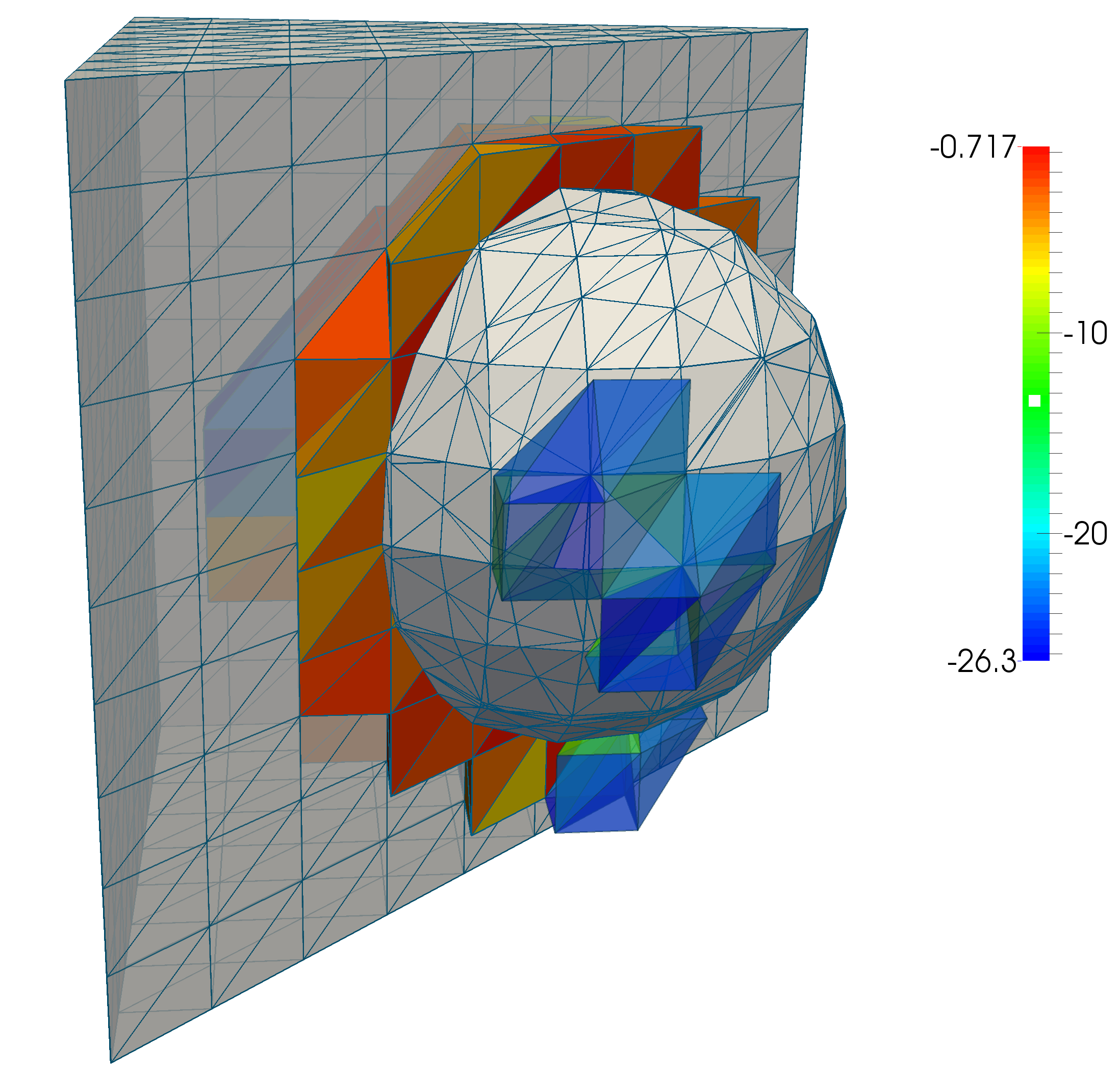
Figure 3: (Left) Principal experimental set-up to study the sensitivity of the conditon number with respect to the relative $\Gamma$ position. (Right): Snapshot of an intersection configuration when moving $\Gamma$ through the background mesh. To visualize “extreme” cut configurations, the color map plots for each intersected mesh element $T$ the value of $\log(\Gamma^{h}\cap T/\operatorname{diam}(T)^{2})$. Thus blue-colored elements contain only an extremely small fraction of the surface.

For $\delta=l/500$, $l=0,\ldots,500$, we compute the condition number $\kappa_{\delta}(\mathcal{A})$ as the ratio of the absolute value of the largest (in modulus) and smallest (in modulus), non-zero eigenvalue. The resulting condition numbers are displayed in Figure 4 as a function of $\delta$. Choosing the stabilization parameters as in the convergence study for the fully stabilized cutDG method, we observe that the position of $\Gamma$ relative to the background mesh $\mathcal{T}_{k}$ has very little effect on the condition number. After turning off either of the bulk and surface related cutFEM stabilizations, the condition number is highly sensitive to the relative position of $\Gamma$ and clearly unbounded as a function of $\delta$.

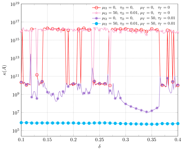
Figure 4: Condition numbers plotted as a function of the position parameter $\delta$. When turning off either the surface or bulk related ghost-penalties (or both), the condition number is highly sensitive to the relative surface positioning in the background mesh. With all ghost penalties activated, the condition number is completely robust.

6 Acknowledgments

This work was supported in part by the Kempe foundation (JCK-1612). The author expresses his gratitude to Ceren Gürkan for her help with the set-up of the convergence experiment, to Erik Burman for his great editorial assistance during the preparation of this contribution, and finally, to the two anonymous referees for their valuable comments and suggestions.

References

- Bastian and Engwer [2009] P. Bastian and C. Engwer. An unfitted finite element method using discontinuous Galerkin. Internat. J. Numer. Meth. Engrg, 79(12):1557–1576, 2009.
- Burman and Hansbo [2010] E. Burman and P. Hansbo. Fictitious domain finite element methods using cut elements: I. A stabilized Lagrange multiplier method. Comput. Methods Appl. Mech. Engrg., 2010.
- Burman and Hansbo [2012] E. Burman and P. Hansbo. Fictitious domain finite element methods using cut elements: II. A stabilized Nitsche method. Appl. Numer. Math., 62(4):328–341, 2012.
- Burman and Hansbo [2013] E. Burman and P. Hansbo. Fictitious domain methods using cut elements: III. A stabilized Nitsche method for Stokes’ problem. ESAIM, Math. Model. Num. Anal., page 19, 2013.
- Burman et al. [2015a] E. Burman, S. Claus, P. Hansbo, M. G. Larson, and A. Massing. CutFEM: discretizing geometry and partial differential equations. Internat. J. Numer. Meth. Engrg, 104(7):472–501, November 2015a.
- Burman et al. [2015b] E. Burman, S. Claus, and A. Massing. A stabilized cut finite element method for the three field Stokes problem. SIAM J. Sci. Comput., 37(4):A1705–A1726, 2015b. doi: 10.1137/140983574. URL http://dx.doi.org/10.1137/140983574.
- Burman et al. [2015c] E. Burman, P. Hansbo, and M. G. Larson. A stabilized cut finite element method for partial differential equations on surfaces: The Laplace–Beltrami operator. Comput. Methods Appl. Mech. Engrg., 285:188–207, 2015c.
- Burman et al. [2016] E. Burman, P. Hansbo, M. G. Larson, and A. Massing. Cut Finite Element Methods for Partial Differential Equations on Embedded Manifolds of Arbitrary Codimensions. ArXiv e-prints, October 2016.
- Burman et al. [2016] E. Burman, P. Hansbo, M. G. Larson, and A. Massing. A cut discontinuous Galerkin method for the Laplace–Beltrami operator. IMA J. Numer. Anal., 37(1):138–169, 2016. doi: 10.1093/imanum/drv068.
- Burman et al. [2016] E. Burman, P. Hansbo, M. G. Larson, A. Massing, and S. Zahedi. Full gradient stabilized cut finite element methods for surface partial differential equations. Comput. Methods Appl. Mech. Engrg., 310:278–296, October 2016. ISSN 0045-7825. doi: http://dx.doi.org/10.1016/j.cma.2016.06.033. URL http://www.sciencedirect.com/science/article/pii/S0045782516306703.
- Burman et al. [2016] E. Burman, P. Hansbo, M.G. Larson, and S. Zahedi. Cut finite element methods for coupled bulk-surface problems. Numer. Math., 133:203–231, 2016.
- Elliott and Ranner [2013] C. M. Elliott and T. Ranner. Finite element analysis for a coupled bulk–surface partial differential equation. IMA Journal of Numerical Analysis, 33(2):377–402, 2013.
- Ern and Guermond [2006] A. Ern and J.-L. Guermond. Evaluation of the condition number in linear systems arising in finite element approximations. ESAIM: Math. Model. Num. Anal., 40(1):29–48, 2006.
- Formaggia et al. [2013] L. Formaggia, A. Fumagalli, A. Scotti, and P. Ruffo. A reduced model for Darcy’s problem in networks of fractures. ESAIM: Mathematical Modelling and Numerical Analysis, 48(4):1089–1116, 07 2013. doi: 10.1051/m2an/2013132.
- Ganesan and Tobiska [2009] Sashikumaar Ganesan and Lutz Tobiska. A coupled arbitrary lagrangian–eulerian and lagrangian method for computation of free surface flows with insoluble surfactants. Journal of Computational Physics, 228(8):2859–2873, 2009.
- Gilbarg and Trudinger [2001] D. Gilbarg and N. S. Trudinger. Elliptic Partial Differential Equations of Second Order. Classics in Mathematics. Springer-Verlag, Berlin, 2001.
- Grande and Reusken [2016] Jörg Grande and Arnold Reusken. A higher order finite element method for partial differential equations on surfaces. SIAM Journal on Numerical Analysis, 54(1):388–414, 2016.
- Groß and Reusken [2011] S. Groß and A. Reusken. Numerical methods for two-phase incompressible flows, volume 40. Springer, 2011.
- Groß and Reusken [2013] S. Groß and A. Reusken. Numerical simulation of continuum models for fluid-fluid interface dynamics. The European Physical Journal Special Topics, 222(1):211–239, 2013.
- Groß et al. [2015] S. Groß, M. A. Olshanskii, and A. Reusken. A trace finite element method for a class of coupled bulk-interface transport problems. ESAIM: Math. Model. Numer. Anal., 49(5):1303–1330, Sept. 2015. doi: 10.1051/m2an/2015013.
- Guzmán and Olshanskii [2017] Johnny Guzmán and Maxim Olshanskii. Inf-sup stability of geometrically unfitted Stokes finite elements. To appear in Math. Comp., 2017. doi: https://doi.org/10.1090/mcom/3288.
- Hansbo et al. [2014] P. Hansbo, M. G. Larson, and S. Zahedi. A cut finite element method for a Stokes interface problem. Appl. Numer. Math., 85:90–114, 2014.
- Hansbo et al. [2015] P. Hansbo, M. G. Larson, and S. Zahedi. Characteristic cut finite element methods for convection–diffusion problems on time dependent surfaces. Comput. Methods Appl. Mech. Engrg., 293:431–461, 2015.
- Hansbo et al. [2016] P. Hansbo, M. G. Larson, and S. Zahedi. A cut finite element method for coupled bulk-surface problems on time-dependent domains. Comput. Methods Appl. Mech. Engrg., 307:96–116, 2016.
- Heimann et al. [2013] F. Heimann, C. Engwer, O. Ippisch, and P. Bastian. An unfitted interior penalty discontinuous Galerkin method for incompressible Navier–Stokes two–phase flow. Internat. J. Numer. Methods Fluids, 71(3):269–293, 2013.
- Johansson and Larson [2013] A. Johansson and M.G. Larson. A high order discontinuous Galerkin Nitsche method for elliptic problems with fictitious boundary. Numer. Math., 123(4), 2013.
- Martin et al. [2005] V. Martin, J. Jaffré, and J.E. Roberts. Modeling fractures and barriers as interfaces for flow in porous media. SIAM Journal on Scientific Computing, 26(5):1667–1691, 2005.
- Massing [2012] A. Massing. Analysis and Implementation of Finite Element Methods on Overlapping and Fictitious Domains. PhD thesis, Department of Informatics, University of Oslo, 2012.
- Massing et al. [2014] A. Massing, M.G. Larson, A. Logg, and M.E. Rognes. A stabilized Nitsche fictitious domain method for the Stokes problem. J. Sci. Comput., 61(3):604–628, 2014. doi: 10.1007/s10915-014-9838-9.
- Massing et al. [2016] A. Massing, B. Schott, and W. A. Wall. A stabilized Nitsche cut finite element method for the Oseen problem. arXiv preprint arXiv:1611.02895, 2016.
- Massjung [2012] R. Massjung. An unfitted discontinuous Galerkin method applied to elliptic interface problems. SIAM Journal on Numerical Analysis, 50(6):3134–3162, 2012.
- Müller et al. [2016] B. Müller, S. Krämer-Eis, F. Kummer, and M. Oberlack. A high-order Discontinuous Galerkin method for compressible flows with immersed boundaries. International Journal for Numerical Methods in Engineering, pages n/a–n/a, 2016. ISSN 1097-0207. doi: 10.1002/nme.5343. URL http://dx.doi.org/10.1002/nme.5343. nme.5343.
- Muradoglu and Tryggvason [2008] Metin Muradoglu and Gretar Tryggvason. A front-tracking method for computation of interfacial flows with soluble surfactants. Journal of computational physics, 227(4):2238–2262, 2008.
- Novak et al. [2007] I. L. Novak, F. Gao, Y.-S. Choi, D. Resasco, J. C. Schaff, and B. M. Slepchenko. Diffusion on a curved surface coupled to diffusion in the volume: Application to cell biology. Journal of computational physics, 226(2):1271–1290, 2007.
- Olshanskii and Reusken [2010] M. A. Olshanskii and A. Reusken. A finite element method for surface PDEs: matrix properties. Numer. Math., 114(3):491–520, 2010.
- Olshanskii et al. [2009] M. A. Olshanskii, A. Reusken, and J. Grande. A finite element method for elliptic equations on surfaces. SIAM J. Numer. Anal., 47(5):3339–3358, 2009.
- Olshanskii et al. [2014] M. A. Olshanskii, A. Reusken, and X. Xu. An Eulerian space-time finite element method for diffusion problems on evolving surfaces. SIAM J. Numer. Anal., 52(3):1354–1377, 2014.
- Rätz [2015] A. Rätz. Turing-type instabilities in bulk–surface reaction–diffusion systems. Journal of Computational and Applied Mathematics, 289:142–152, 2015.
- Saye [2015] R. I. Saye. High-order quadrature methods for implicitly defined surfaces and volumes in hyperrectangles. SIAM Journal on Scientific Computing, 37(2):A993–A1019, 2015.
- Schott [2017] B. Schott. Stabilized Cut Finite Element Methods for Complex Interface Coupled Flow Problems. PhD thesis, Technical University of Munich, 2017.
- Sollie et al. [2011] W. E. H. Sollie, O. Bokhove, and J. J. W. van der Vegt. Space–time discontinuous Galerkin finite element method for two-fluid flows. J. Comput. Phys., 230(3):789–817, 2011.
- Winter et al. [2017] M. Winter, B. Schott, A. Massing, and W.A. Wall. A Nitsche cut finite element method for the Oseen problem with general Navier boundary conditions. arXiv preprint arXiv:1706.05897, 2017.