Classification of geometrical objects by integrating currents and functional data analysis

Abstract

This paper focuses on the application of Linear Discriminant Analysis to a set of geometrical objects (bodies) characterized by currents. A current is a relevant mathematical object to model geometrical data, like hypersurfaces, through integration of vector fields along them. As a consequence of the choice of a vector-valued Reproducing Kernel Hilbert Space (RKHS) as a test space to integrate over hypersurfaces, it is possible to consider that hypersurfaces are embedded in this Hilbert space. This embedding enables us to consider classification algorithms of geometrical objects.
A method to apply Functional Discriminant Analysis in the obtained vector-valued RKHS is given. This method is based on the eigenfunction decomposition of the kernel. So, the novelty of this paper is the reformulation of a size and shape classification problem in Functional Data Analysis terms using the theory of currents and vector-valued RKHS.
This approach is applied to a 3D database obtained from an anthropometric survey of the Spanish child population with a potential application to online sales of children’s wear.

keyword Currents; Statistical Shape and Size Analysis; Reproducing Kernel Hilbert Space; Functional Data Analysis; Discriminant Analysis.

1 Introduction

Supervised classification of geometrical objects ([Ripley(2007)]), i.e. the automated assigning of geometrical objects to pre-defined classes, is a common problem in many scientific fields. This is a difficult task where several challenges have to be addressed.

The first challenge is how to handle this kind of data from a mathematical point of view. Several mathematical frameworks have been proposed to deal with geometrical data, and three of them are the most widely used. As a first option, functions can be used to represent closed contours of the objects (curves in 2D and surfaces in 3D) ([Younes(1998)]). Geometrical objects can also be treated as subsets of $\mathbb{R}^{n}$ ([Serra(1982), Stoyan and Stoyan(1994)]), or finally they can be described as sequences of points that are given by certain geometrical or anatomical properties (landmarks) ([Kendall et al(2009)Kendall, Barden, Carne, and Le, Dryden and Mardia(2016)]).

These approaches are, in general, known as Shape or Size and Shape Analysis and in these settings, the objects are usually embedded into a space which is not a vector space (in many cases it is a smooth manifold) and on which the geodesic distance as a natural metric is difficult to compute. This makes the definition of statistics particularly difficult; for example, there is no simple, explicit way to compute a mean ([Pennec(2006), Vinué et al(2016)Vinué, Simó, and Alemany, Flores et al(2016)Flores, Gual-Arnau, Ibáñez, and Simó]).

In our approach, the contour of each geometrical object (curve in $\mathbb{R}^{2}$, surface in $\mathbb{R}^{3}$, or hypersurface in $\mathbb{R}^{n}$), is firstly represented by a mathematical structure named current ([Vaillant and Glaunès(2005), Glaunès and Joshi(2006)]). Next, each current is associated to an element of a vector valued Reproducing Kernel Hilbert Space (RKHS) by duality ([Durrleman(2010), Barahona et al(2017)Barahona, Gual-Arnau, Ibáñez, and Simó]). This modeling is weakly sensitive to the sampling of shapes and it does not depend on the choice of parameterizations.

In this paper, we propose a method to apply Discriminant Analysis ([Fisher(1936)]) to this kind of data, i.e. to a sample of curves or surfaces (hypersurfaces in general), which are represented by functions in a vector valued RKHS. For this purpose, Functional Data Analysis (FDA) techniques will be adapted to the case of being working on an RKHS.

The theory of statistics with functional data has become increasingly popular since the end of the 1990s and is now a major field of research in statistics. It is used when the sample space is an infinite-dimensional function space. Although this theory has incorporated many tools from classic parametric or multivariate statistics, the infinite-dimensional nature of the sample space poses particular problems. The books by [Silverman and Ramsay(2005)] and [Ferraty and Vieu(2006)] are key references in the FDA literature.

Regarding Functional Discriminant Analysis, [Hall et al(2001)Hall, Poskitt, and Presnell] use functional principal coordinates to reduce the dimension and then apply both a non-parametric kernel and Gaussian-based discriminators to the dimension-reduced data.

Key references on the particular case of Functional Linear Discriminant Analysis (FLDA) are [James and Hastie(2001)] and [Preda et al(2007)Preda, Saporta, and Lévéder]. As an extension of the classical multivariate approach, the aim of FLDA is finding linear combinations such that the between-class variance is maximized with respect to the total variance, but, due to the infinite-dimensional nature of the data, standard LDA can’t be used directly. If the functional data have been observed on every point of their domains, one could discretize the domain of the functions to avoid this obstacle. However, doing so usually leads to high-dimensional data that is highly correlated, so this makes estimating the within-class covariance matrix problematic. Usually, the problem can be overcome by using some form of regularization and/or projection of each functional data onto a finite-dimensional space. Then, one can use LDA on the coefficients of the data in this space, as they are a finite-dimensional representation of the infinite-dimensional functional data.

The method that we propose follows the habitual steps of FLDA but for it, several important difficulties have to be overcome. The first problem is given by the fact that, although our data are functional, they are not expressed in the usual way. We propose to solve this problem by using regularization theory ([Cucker and Smale(2001), Bickel et al(2006)Bickel, Li, Tsybakov, van de Geer, Yu, Valdés, Rivero, Fan, and van der Vaart]). Secondly, our functions are vector-valued and they are in a vector-valued RKHS. For this reason we propose to express each vector field with respect to the orthonormal basis given by the eigenfunction decomposition of the kernel that defines the RKHS. This decomposition can be obtained as a generalization of the similar results to the scalar case ([Quang et al(2010)Quang, Kang, and Le]). The coefficients are estimated and the vector associated with each vector field is obtained. The elements of the basis given by the eigenfunction decomposition of the kernel are orthonormal and ordered following an optimality approximation criterion. These properties allow us to reduce the dimension and then we are able to apply the standard LDA algorithm, as in the multivariate case.

In order to show the applicability of the proposed methodology, we are going to test it on a well known data set of 2D synthetic figures and on a real data set of 3D anthropometric data of Spanish children. Our implementations have been written in [MATLAB(2015)].

The article is organized as follows: Section 2 concerns the theoretical concepts of currents and Reproducing Kernel Hilbert Spaces. In Section 3 we use the representation of vector fields in the sample with respect to an orthonormal basis in the RKHS to apply the Discriminant Analysis algorithm. An experimental study with synthetic figures is conducted in Section 4. The application for assigning a size to each child according to his/her body size and shape is detailed in Section 5. Finally, conclusions are discussed in Section 6.

2 Embedding our data in a vector valued Reproducing Kernel Hilbert Space

As stated in the introduction, geometrical objects to be classified are embedded in a particular function space. The motivation for this embedding is the idea of “currents”, which involves characterizing a shape via its “action” when integrating over vector fields. Seminal papers about currents are [Rham(1960)] and [Federer and Fleming(1960)]. This characterization of shapes (mainly curves and surfaces) as currents is studied in detail, for instance, in [Durrleman et al(2009)Durrleman, Pennec, Trouvé, and Ayache], [Durrleman(2010)] and [Barahona et al(2017)Barahona, Gual-Arnau, Ibáñez, and Simó]. In this section we revise the main results.

Let $D$ be a compact set in $\mathbb{R}^{n}$ and let $X$ be the contour of the geometrical object of interest. We assume that $X$ is a piecewise-defined smooth and oriented hypersurface in $D$ and that $\tau(x)$ is the vector associated with the $(n-1)$-multivector defined by a basis of the tangent space $T_{x}X$ (defined almost everywhere).

Let $K:D\times D\longrightarrow\mathbb{R}^{n\times n}$ be a matrix valued kernel and $H_{K}(D,\mathbb{R}^{n})$ its associated vector-valued RKHS with inner product $\langle\,\,,\,\,\rangle_{H_{K}}$.

We consider the function defined from the integral:

$$C_{X}(y)=\int_{X}K(x,y)\tau(x)\,dx.$$

In the particular case where $X$ is a piecewise-defined smooth curve $L$ in $\mathbb{R}^{2}$, $\tau(x)$ is the tangent vector to $L$ at point $x$ of the curve in $\mathbb{R}^{2}$. Similarly, if $X$ is a piecewise-defined smooth surface $S$ in $\mathbb{R}^{3}$, $\tau(x)$ is the normal to the surface $S$ at point $x$.

The “shape” of the object will be identified with the function $C_{X}:D\longrightarrow\mathbb{R}^{n}$, that is, we deal with hypersurfaces as vector fields in $H_{K}(D,\mathbb{R}^{n})$.

The choice of the kernel determines the vector-valued RKHS, and especially its inner product. Although it is not known how to choose the “best” kernel for a given application (see Appendix B of [Durrleman(2010)]), translation-invariant isotropic matrix kernels, defined from translation-invariant isotropic scalar kernels of the form $k(x,y)=k(\left\lVert x-y\right\rVert_{\mathbb{R}^{n}})$ are often used.

A matrix valued kernel of particular importance is the vector-valued Gaussian kernel:

$$K(x,y):=k(x,y)\,{\mathbb{I}}_{n\times n}=\displaystyle e^{\displaystyle-\frac{\left\lVert x-y\right\rVert^{2}_{\mathbb{R}^{n}}}{\lambda^{2}}}{\mathbb{I}}_{n\times n},$$ (1)

where ${\mathbb{I}}_{n\times n}$ is the identity matrix and $\lambda>0$ is a scale parameter (bandwidth). This is the matrix valued kernel that we will use in our experiments.
Details about the choice of the value of the parameter $\lambda$, and a comparative study between kernels, regarding unsupervised classification, can be found in [Barahona et al(2017)Barahona, Gual-Arnau, Ibáñez, and Simó].

2.1 Discrete setting

In the discrete setting, the vectors $\tau(x)$ are constant over each mesh cell. Then, if $x_{j}$ is located at the center of mass of mesh cell $j$, and $\tau_{j}$ is $\tau(x_{j})$ scaled by the size of the mesh cell,

$$X\longrightarrow C_{X}\cong\int_{X}K(x,\cdot)\tau(x)\,dx\approx\sum_{j}K(x_{j},\cdot)\tau_{j},$$

and if $\varphi_{1}=\displaystyle\sum_{j=1}^{N_{1}}K(x^{1}_{j},\cdot)\tau^{1}_{j}$ and $\varphi_{2}=\displaystyle\sum_{j=1}^{N_{2}}K(x^{2}_{j},\cdot)\tau^{2}_{j}$ are two ‘hypersurfaces’, their inner product is

$$\langle\varphi_{1},\varphi_{2}\rangle_{H_{K}}=\displaystyle\sum_{i=1}^{N_{1}}\sum_{j=1}^{N_{2}}\tau^{1}_{i}\cdot K(x^{1}_{i},x^{2}_{j})\tau^{2}_{j},$$

where $\cdot$ in this expression denotes the inner product in $\mathbb{R}^{n}$.

If $L$ is a planar curve and $\{y_{1},y_{2},\ldots,y_{p}\}$ is a discretization of $L$, then $L$ can be represented as a vector field $\sum K(x_{j},\cdot)\tau_{j}$, where $x_{j}$ denotes the center of the segment $[y_{j},y_{j+1}]$ and $\tau_{j}$ is the vector $y_{j+1}-y_{j}$, which is an approximation of the tangent vector.

If $S$ is a surface in $\mathbb{R}^{3}$ and we have a triangulation of $S$, then $S$ can be represented as a vector field $\sum K(x_{j},\cdot)\tau_{j}$, where $x_{j}$ are the barycenters of the triangles and $\tau_{j}$ are their area vectors (that is, their unit normal vectors, scaled by their area).

3 Discriminant Analysis in an RKHS for hypersurface classification

We have seen in the previous section how to transform geometrical objects into elements of a vector-valued RKHS (a space of vector fields), therefore, we assume that we have a random sample of size $m$ of vector fields such as:

$$\varphi_{k}(\cdot)=\displaystyle\sum_{i=1}^{N_{k}}K(x^{k}_{i},\cdot)\tau^{k}_{i}\in H_{K}(D,\mathbb{R}^{n}),\,\,k=1,\dots,m,$$ (2)

Because our data are a particular type of vector-valued functions, it seems logical to use the theory of Functional Data Analysis (FDA) and, in particular, Functional Discriminant Analysis for this purpose.

Most applications of FDA are based on applying regularization methods and expressing functional data on an orthonormal basis of functions. This removes the noise, reduces the dimension and allows to use classical multivariate methods. The use of this type of techniques for our data and for our particular space of functions presents several differences and difficulties.

Firstly, our data are not expressed in the standard form of functional data. They are defined from the points $x^{k}_{i}$ where the kernel is evaluated (Eq. 2) and these points are different from one hypersurface (geometrical object) to another.

Secondly, because our space is an RKHS, we must make use of the properties of these spaces to find the most appropriate orthonormal basis in which to project our data. The properties of RKHS are well known and largely used in the scalar case, but our functions are vector-valued, and the vector-valued RKHS are not as well known and many of their properties are still open problems in the functional analysis literature.

These two issues are addressed in the following subsections.

3.1 Representing the vector fields in the same sample grid of points

Let us consider the vector field $\varphi_{k}(\cdot)$ associated with the discretized hypersurface $X_{k}$ in $D$, given by Eq.  (2) and being $\{x^{k}_{i}\}_{i=1}^{N_{k}}$ the centers of mass of the respective mesh cells.

Let $\{a_{i}\}_{i=1}^{N}$ be a sample grid in $D$, the “Representer Theorem” ([Cucker and Smale(2001)]) tell us that for each vector field $\varphi_{k}$ there exist a unique mapping $\overline{\varphi_{k}}\colon\mathbb{R}^{n}\rightarrow\mathbb{R}^{n}$ such that:

$$\overline{\varphi_{k}}=\operatorname*{arg\,min}_{g\in H_{K}(D,\mathbb{R}^{n})}\frac{1}{N}\sum_{i=1}^{N}\left\lVert g(a_{i})-b_{k,i}\right\rVert_{\mathbb{R}^{n}}^{2}+\gamma\left\lVert g\right\rVert_{H_{K}}^{2}$$ (3)

where $b_{k,i}:=\varphi_{k}(a_{i})$, $b_{k,i}=(b_{k,i}^{1},b_{k,i}^{2},\ldots,b_{k,i}^{n})\in\mathbb{R}^{n}$ and $\gamma>0$ a regularizing parameter. This way, we can obtain a function that is as smooth as we need (it depends on the choice of $\gamma$) and which fits the data, i.e. $\overline{\varphi_{k}}(a_{i})$ is close to $\varphi_{k}(a_{i})$.

In the experimental study, we choose different values of $\gamma$ and select the appropriate parameter value by checking the performance of the classification.

Moreover, the unique solution $\overline{\varphi_{k}}$ to Eq. (3) has the expression $\overline{\varphi_{k}}(\cdot)=\displaystyle\sum_{i=1}^{N}K(a_{i},\cdot)(\beta_{k,i})$, where vectors $\beta_{k,i}\in\mathbb{R}^{n}$ are obtained by solving the following matrix system:

$$(\gamma\,N\,{\mathbb{I}}_{N\times N}+K|_{a})\beta_{k}=b_{k},$$

with $K|_{a}$ the matrix defined as $K|_{a}(i,j)=k(a_{i},a_{j})\in\mathbb{R}$, $i,j=1,\ldots,N$, and $\beta_{k}$, $b_{k}$ are the following $N\times n$ matrices

$$\beta_{k}=\left(\begin{array}[]{cccc}\beta_{k,1}^{1}&\beta_{k,1}^{2}&\ldots&\beta_{k,1}^{n}\\ \beta_{k,2}^{1}&\beta_{k,2}^{2}&\ldots&\beta_{k,2}^{n}\\ \vdots&\vdots&\ldots&\vdots\\ \vdots&\vdots&\ldots&\vdots\\ \beta_{k,N}^{1}&\beta_{k,N}^{2}&\ldots&\beta_{k,N}^{n}\\ \end{array}\right);\textup{ }b_{k}=\left(\begin{array}[]{cccc}b_{k,1}^{1}&b_{k,1}^{2}&\ldots&b_{k,1}^{n}\\ b_{k,2}^{1}&b_{k,2}^{2}&\ldots&b_{k,2}^{n}\\ \vdots&\vdots&\ldots&\vdots\\ \vdots&\vdots&\ldots&\vdots\\ b_{k,N}^{1}&b_{k,N}^{2}&\ldots&b_{k,N}^{n}\\ \end{array}\right).$$

As a result of applying this theorem to all the vector fields of our sample, from now on we will work with a sample of vector fields of the type:

$$\overline{\varphi_{k}}(\cdot)=\displaystyle\sum_{i=1}^{N}K(a_{i},\cdot)\beta_{k,i}\in H_{K}(D,\mathbb{R}^{n}),\,k=1,\dots,m.$$

3.2 Orthonormal basis in $H_{K}(D,\mathbb{R}^{n})$

In this section we investigate how to obtain an appropriated orthonormal basis of the vector-valued RKHS $H_{K}(D,\mathbb{R}^{n})$ where project our data. Final projections will be truncated in an optimal way to obtain a finite dimensional approximation, which enables us the use of multivariate discriminant analysis.

Let us consider the Hilbert space $L^{2}(D,\mathbb{R}^{n}):=\{f=(f_{1},\dots,f_{n})\colon D\longrightarrow\mathbb{R}^{n}\,/\,\left\lVert f\right\rVert^{2}_{L^{2}(D,\mathbb{R}^{n})}=\sum_{i=1}^{n}\int_{D}\left\lvert f_{i}(x)\right\rvert^{2}\,dx<\infty\}$ and the integral operator, $L_{K,D}\colon L^{2}(D,\mathbb{R}^{n})\longrightarrow L^{2}(D,\mathbb{R}^{n})$, defined by

$$L_{K,D}f(x)=\int_{D}K(x,y)(f(y))\,dy=\left(\int_{D}k(x,y)f_{i}(y)\,dy\right)_{i=1}^{n}=(L_{k}f_{i}(x))_{i=1}^{n}.$$

It is easy to check that we have the conditions to ensure that the integral operator $L_{K,D}$ is self-adjoint, compact, and positive, since each component $L_{k}$ will be.

Let $\{\lambda_{l}\}_{l=1}^{\infty}$ be the eigenvalues of the integral operator $L_{k}$ and the corresponding eigenfunctions $\{\phi_{l}\}_{l=1}^{\infty}$. The spectral theorem implies that $\lambda_{1}\geq\lambda_{2}\geq\dots\geq 0$ and $\displaystyle\lim_{l\rightarrow\infty}\lambda_{l}=0$ (see [Hsing and Eubank(2015)]).

If $\phi_{l}$ is an eigenfunction of $L_{k}$ with corresponding eigenvalue $\lambda_{l}$, then $\psi_{l}^{j}=(0,\dots,\phi_{l},\dots,0)$, where $\phi_{l}$ is placed at position $j$, is an eigenfunction of $L_{K,D}$ corresponding to the same eigenvalue.

Theorem 3.1

Let $\overline{\varphi_{k}}(\cdot)=\displaystyle\sum_{i=1}^{N}K(\cdot,a_{i})(\beta_{k,i})$ be a vector field representing a hypersurface $X_{k}$ in $\mathbb{R}^{n}$. Then, $\overline{\varphi_{k}}$ can be expressed as

$$\overline{\varphi_{k}}(\cdot)=\displaystyle\sum_{j=1}^{n}\sum_{l=1}^{\infty}\mu^{j}_{l,k}\left(\sqrt{\lambda_{l}}\psi^{j}_{l}(\cdot)\right),$$ (5)

where $\{\{\sqrt{\lambda_{l}}\psi_{l}^{j}\}_{l=1}^{\infty}\}_{j=1}^{n}$ is an orthonormal basis for $H_{K}(D,\mathbb{R}^{n})$.

Furthermore, the first $d=\operatorname{rank}(K|_{a})$ coefficients $\mu^{j}_{l,k}$ can be approximated by

$$\widehat{\mu^{j}_{l,k}}=\sqrt{\ell_{l}}(v_{l}\cdot\beta_{k}^{j})$$

for $j=1,\ldots,n$, where $v_{l}\in\mathbb{R}^{N}$ are the eigenvectors of $K|_{a}$, $\ell_{l}$ are the eigenvalues of $K|_{a}$ and $\beta_{k}^{j}=(\beta_{k,1}^{j},\beta_{k,2}^{j},\ldots,\beta_{k,N}^{j})$.

Proof. Consider now a vector field:

$$\overline{\varphi_{k}}(\cdot)=\displaystyle\sum_{i=1}^{N}K(a_{i},\cdot)(\beta_{k,i})=\left(\sum_{i=1}^{N}k(a_{i},\cdot)\beta^{1}_{k,i},\dots,\sum_{i=1}^{N}k(a_{i},\cdot)\beta^{n}_{k,i}\right).$$

Then, for $x\in D$, and from [Quang et al(2010)Quang, Kang, and Le], we have

$$\overline{\varphi_{k}}(x)=\sum_{i=1}^{N}K(a_{i},x)(\beta_{k,i})=\sum_{i=1}^{N}\sum_{l=1}^{\infty}\lambda_{l}\phi_{l}(a_{i})\phi_{l}(x)\beta_{k,i}.$$

Therefore,

$$\overline{\varphi_{k}}(x) =\left(\sum_{i=1}^{N}\sum_{l=1}^{\infty}\lambda_{l}\phi_{l}(a_{i})\phi_{l}(x)\beta_{k,i}^{1},\dots,\sum_{i=1}^{N}\sum_{l=1}^{\infty}\lambda_{l}\phi_{l}(a_{i})\phi_{l}(x)\beta_{k,i}^{n}\right)$$

$$=\left(\sum_{l=1}^{\infty}\lambda_{l}\left(\sum_{i=1}^{N}\phi_{l}(a_{i})\beta_{k,i}^{1}\right)\phi_{l}(x),\dots,\sum_{l=1}^{\infty}\lambda_{l}\left(\sum_{i=1}^{N}\phi_{l}(a_{i})\beta_{k,i}^{n}\right)\phi_{l}(x)\right)$$

$$=\left(\sum_{l=1}^{\infty}\mu^{1}_{l,k}\left(\sqrt{\lambda_{l}}\phi_{l}(x)\right),\dots,\sum_{l=1}^{\infty}\mu^{n}_{l,k}\left(\sqrt{\lambda_{l}}\phi_{l}(x)\right)\right)$$

where $\mu_{l,k}^{j}=\displaystyle\sqrt{\lambda_{l}}\sum_{i=1}^{N}\phi_{l}(a_{i})\beta_{k,i}^{j}$, $j=1,\dots,n$. Again from [Quang et al(2010)Quang, Kang, and Le], $\{\{\sqrt{\lambda_{l}}\psi_{l}^{j}\}_{l=1}^{\infty}\}_{j=1}^{n}$ is an orthonormal basis for $H_{K}(D,\mathbb{R}^{n})$; therefore, for $x\in D$,

$$\overline{\varphi_{k}}(x)=\sum_{j=1}^{n}\sum_{l=1}^{\infty}\mu^{j}_{l,k}\left(\sqrt{\lambda_{l}}\psi^{j}_{l}(x)\right).$$

On the other hand, following the works of [González and Muñoz(2010)] and [Smale and Zhou(2009)], each $\phi_{l}(a_{i})$ can be approximated by $\sqrt{N}v_{l,i}$, where $v_{l}=\{v_{l,1},\dots,v_{l,N}\}$ is the $l$-th eigenvector of the matrix $K|_{a}$. In addition, $\lambda_{l}$ can be estimated by $\ell_{l}/N$, where $\ell_{l}$ is the eigenvalue of $K|_{a}$ corresponding to $v_{l}$. Therefore

$$\widehat{\mu_{l,k}^{j}}=\sqrt{\ell_{l}}\sum_{i=1}^{N}v_{l,i}\beta_{k,i}^{j}=\sqrt{\ell_{l}}(v_{l}\cdot\beta_{k}^{j}).\quad\square$$

In addition, it is known ([[, see Theorems 4.4.7 and 4.6.8 in]]Hsing15) that for a fixed integer $r>0$ :

$$\min_{f_{1},\dots,f_{r}\in H_{K}(D,\mathbb{R}^{n})}\int\int_{D\times D}\left(K(y,x)-\sum_{j=1}^{n}\sum_{l=1}^{\infty}f_{l}^{j}(y)f_{l}^{j}(x)\right)^{2}dydx=\sum_{j=r+1}^{\infty}\lambda_{j}^{2},$$

where the minimum is achieved by $\sum_{l=1}^{r}\psi^{j}_{l}(y)\psi^{j}_{l}(x)$. That is to say, as our functional data are of the form $\sum_{j=1}^{n}\sum_{l=1}^{\infty}\mu^{j}_{l,k}\left(\sqrt{\lambda_{l}}\psi^{j}_{l}(x)\right)$, and the truncated eigenvalue-eigenvector decomposition provides the best approximation to $K$, the truncation of this representation reduces the dimension in an optimal way.

Then, if we truncate the second summation in the Eq. (5) at $d=\operatorname{rank}(K|_{a})$, each hypersurface $X_{k}$ for $k=1,\ldots,m$, is given by the coefficients $\mu^{j}_{l,k}$ for $j=1,\ldots,n$ and $l=1,\ldots,d$ (estimated by $\widehat{\mu_{l,k}^{j}}$), on the orthonormal basis $\{\{\sqrt{\lambda_{l}}\psi_{l}^{j}\}_{l=1}^{\infty}\}_{j=1}^{n}$. As a result, it can be represented as the $(n\cdot d)$-dimensional vector

$$\mu_{k}=(\widehat{\mu_{1,k}^{1}},\widehat{\mu_{1,k}^{2}},\ldots,\widehat{\mu_{1,k}^{n}},\widehat{\mu_{2,k}^{1}},\widehat{\mu_{2,k}^{2}},\ldots,\widehat{\mu_{2,k}^{n}},\ldots,\widehat{\mu_{d,k}^{1}},\widehat{\mu_{d,k}^{2}},\ldots\widehat{\mu_{d,k}^{n}})$$ (6)

This expression optimally reduces the infinite-dimensional problem to a finite-dimensional one. Each surface $X_{k}$ is characterized by the ($n\cdot d$)-dimensional vector through association of currents and now, it is possible to apply the classical multivariate Linear Discriminant Analysis method. In particular, in our applications we will use the multivariate LDA algorithm implemented in [MATLAB(2015)].

4 Experimental 2D Study

The public database of synthetic figures “MPEG7 CE Shape-1 PartB” (www.imageprocessingplace.com/root_files_V3/image_databases.htm) contains binary images grouped into categories like cars, faces, watches, horses and birds, with images in the same category showing noticeably different shapes.

In order to illustrate or methodology, three of the categories of this database of synthetic figures are considered: cars, faces and watches. Each class contains $20$ elements, except the watch class, in which two of them are rejected (watch-2 is an atypical element because of its very large size, and watch-8 is considerably tilted and our theoretical framework considers size and shape). In order to have a data set with figures with different sizes, half of the figures from each category were enlarged by a scale factor of $1.5$. Then, $10$ of the figures are labelled as ”group 1” (”small car”); other $10$ as ”group 2” (”large car”); $10$ images are labelled as ”group 3” (”small face”), other $10$ as ”group 4” (”large face”); $8$ images are labelled as ”group 5” (”small watch”) and the $8$ remaining images are labelled as ”group 6” (”large watch”). After this labelling, each figure of the sample was enlarged by a random coefficient ranging between $1$ and $1.1$, in order to change the “height” of the figures somewhat.

The $58$ figures were centered, and the contour $\alpha_{k}$ of each of them defined an oriented smooth curve which was discretized by $100$ points $\{y_{j}^{k}\}_{j=1}^{100}$ ($y_{1}^{k}=y_{100}^{k}$) for $k=1,\ldots,58$. For each $k\in\{1,\ldots,58\}$, we defined the centers of the segments $x_{j}^{k}=(y_{j}^{k}+y_{j+1}^{k})/2$ and the vectors $\tau_{j}^{k}=y_{j+1}^{k}-y_{j}^{k}$, $\forall j=1,\ldots,99$, which define the vector field $\sum_{j=1}^{99}K(x_{j}^{k},\cdot)\tau_{j}^{k}$ in $H_{K}(D,\mathbb{R}^{2})$. Gaussian kernels (Eq. 1) were used in the definition of the matrix valued kernels $K$.

Fig. 1 shows an example of an object from each class. The points $\{x_{j}^{k}\}_{j=1}^{99}$ are plotted in black and the vectors $\{\tau_{j}^{k}\}_{j=1}^{99}$ from each curve are plotted in a different color.

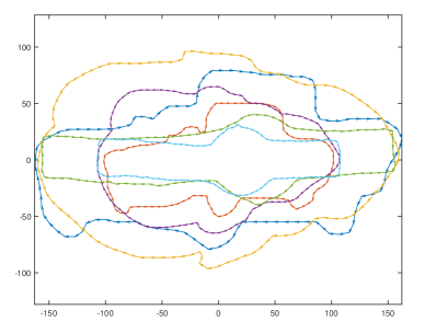
Figure 1: An object from each class from the synthetic 2D database.

To represent each vector field $\sum_{j=1}^{99}K(x_{j}^{k},\cdot)\tau_{j}^{k}$ in relation to a fixed grid using the procedure described in Section 3.1, a grid of $N=3337$ equally spaced points was chosen in $D=[-175,175]\times[-115,115]$, with common vertical and horizontal gap $\Delta=5$.

Once we defined the grid, the coefficients of the vector fields that represent each curve in relation to the orthonormal basis of $H_{K}(D,\mathbb{R}^{2})$ were estimated (Section 3).

Different values for parameters $\lambda$ (Eq. 1), and $\gamma$ (Eq. 3) were chosen. A Functional Discriminant Analysis was conducted and a leave-one-out cross-validation process was carried out to check the performance of the classification obtained, and to select appropriate parameter values.

Table 1 shows the results. As can be seen, results are very satisfactory, as the cross-validation errors are zero for different values of $\lambda$ and $\gamma$. As can be seen in the table, the correct determination of parameter $\lambda$ is more important than the determination of parameter $\gamma$, as $\gamma$ seems less influential in the classification results. The value $67.6$ of the parameter $\lambda$ corresponds to the standard deviation of the points $\{y_{j}^{k}\}_{j=1}^{100}$, $k=1,\ldots,58$ that define the curves of each sample.

$\lambda$	$\gamma$	Cross-validation error
	$1\times 10^{-4}$	$30$ ($51.72\%$)
$1$	$3\times 10^{-4}$	$30$ ($51.72\%$)
	$4\times 10^{-4}$	$30$ ($51.72\%$)
	$1\times 10^{-4}$	$6$ ($10.34\%$)
$2$	$3\times 10^{-4}$	$6$ ($10.34\%$)
	$4\times 10^{-4}$	$6$ ($10.34\%$)
	$1\times 10^{-4}$	$0$
$67.6$	$3\times 10^{-4}$	$0$
	$4\times 10^{-4}$	$0$
	$1\times 10^{-4}$	$0$
$100$	$3\times 10^{-4}$	$0$
	$4\times 10^{-4}$	$0$

Table 1: Table of results of cross-validation from the 2D database.

5 Application to classify children’s body shapes

In 2004, the Biomechanics Institute of Valencia performed an anthropometrical study of the Spanish child population, where a randomly selected sample of Spanish children between the ages of $3$ to $10$ years was scanned using a Vitus Smart 3D body scanner from Human Solutions.

As there is a different size system for each sex, in order to illustrate our procedure the subset of the girls older than 6 was chosen from the whole data set. Children younger than 6 have difficulties in maintaining a standard position during the scanning process, so they were excluded from our data set. The European standard norm UNE-EN 13402-3, defines $4$ different sizes for girls over $6$, (size.6; size.8; size.10 and size.12), corresponding to four consecutive height ranges. This selection resulted in a sample of size $195$ scanned girls, but in the data set does not provide information about the size that better fits to each of them.

In a previous work, [Barahona et al(2017)Barahona, Gual-Arnau, Ibáñez, and Simó] analyzed this data set, and proposed a new sizing system taken into account children’s shape and size, without any previous classification by height. This new sizing system defined $5$ different sizes for girls over $6$, instead of the $4$ sizes defined by the standard norm. These sizes will be denoted by $S1$, $\cdots$, $S5$ , and each girl in the data set, was assigned to one of these new sizes. The median (in mm) of the main anthropometric measurements of the girls of our data set labeled on each size are shown in Table 2. Fig. 2 shows some of the girls labeled as $S1$.

Size	Height	Chest	Waist	Hip	Group
		circumference	circumference	circumference	size
S1	$1241$	$610$	$540$	$661$	$57$
S2	$1259$	$678$	$622$	$754$	$39$
S3	$1362$	$660$	$571.5$	$723.5$	$56$
S4	$1361.5$	$747.5$	$673$	$814$	$34$
S5	$1417$	$832$	$767$	$903$	$9$

Table 2: Median (in mm) of the main antropometric measures of the girls belonging to each size.

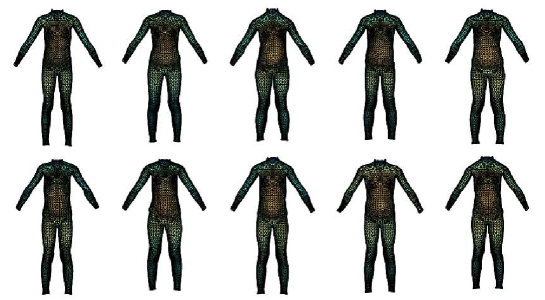
Figure 2: Some of the girls that have the same size.

So, our data set contains a sample of $195$ girls, that have been scanned and assigned to a size (see [Barahona et al(2017)Barahona, Gual-Arnau, Ibáñez, and Simó]), and our aim is to obtain a classification rule that allows us to assign a new girl to her corresponding size, according to this sizing system.

Following the methodology exposed, the body contour from each girl has been represented by an oriented triangulated smooth surface with $4668$ triangles. The center of each oriented triangle with vertices $a_{j}^{k}$, $b_{j}^{k}$ and $c_{j}^{k}$ has been defined as $x_{j}^{k}=(a_{j}^{k}+b_{j}^{k}+c_{j}^{k})/3$, and the normal vectors to the surface are $\tau_{j}^{k}=(b_{j}^{k}-a_{j}^{k})\times(c_{j}^{k}-a_{j}^{k})$, where $j=1,\dots,4668$ denotes the triangles of the surface and $k=1,\cdots,195$ denotes each girl. Then, the $k$-th girl’s body contour is associated with the vector field $\sum_{j=1}^{4668}K(x_{j}^{k},\cdot)\tau_{j}^{k}$ in $H_{K}(D,\mathbb{R}^{3})$, where $D=[-472.73,487.27]\times[-824.72,735.28]\times[-156.70,203.30]$ and $\Delta=120$ (in this case, the grid has $N=504$ points)

Once again, a Gaussian kernel (Eq. 1) is used in the definition of the matrix valued kernel $K$, several suitables values of $\gamma$ are selected, and the value of the parameter $\lambda$ is chosen as the standard deviation of the points $\{x_{j}^{k}\}_{j=1}^{4668}$, $k=1,\ldots,195$ that define the surfaces of each girl.

Using the same procedure as in the 2D database, FLDA was conducted and a leave one out cross-validation procedure was carried out to check the performance of the classification. Table 3 shows the results.

$\lambda$	$\gamma$	$\operatorname{rank}(K)$	CV error
$183.4393$	$1/930$	$504$	$16.92\%$

Table 3: Table of results of the cross-validation analysis ($195$ girls).

The percentage of misclassifications with this FLDA - cross validation analysis is of $16.92\%$, showing a high agreement percentage ($83.08\%$) in the prediction of the right size of girls’ clothing from her body size and shape. These results, are similar or slightly better than the obtained on the studies found in the literature for similar problems of body shape classification of the adult population ([Viktor et al(2006)Viktor, Paquet, and Guo, Devarajan and Istook(2004), Meunier(2000)]), that use linear anthropometrical dimensions or directly the three-dimensional landmark coordinates as input information; clustering analysis for defining sizing systems and classical linear discriminant analysis as supervised classification tool.

6 Discussion

The first aim of this paper has been to adapt and to generalize the linear discriminant analysis methodology for functional data (FLDA) to problems where the data lie on a vector-valued RKHS.

Given a random sample of geometrical objects, each geometrical object (curve or surface), has been represented by a current and each current has been associated to an element (to a function) of a vector-valued RKHS (see Section 2).

The main novelty of the work is exposed in Section (3). Most applications of FDA are based on applying regularization methods and expressing functional data on an orthonormal basis of functions. Therefore, as our data (functions in a vector-valued RKHS), are not expressed in the standard form of functional data, the ’Representer Theorem’ has been used to define all the functions from the same grid of points (Subsection 3.1). Then, it has been necessary to investigate how to obtain an appropriated orthonormal basis of the vector-valued RKHS where project our data (Subsection 3.2).

To check the performance of this methodology, it has been applied on a supervised classification problem on a data set of synthetic figures (Section 4). As an example of application, it has been used to get a classifier of child’s clothing sizes (Section 5). Very good results ($0\%$ and $16.92\%$ cross validation errors respectively) have been obtained in both cases.

7 Acknowledgments

This paper has been partially supported by the project $DPI2013-47279-C2-1-R$ from the Spanish Ministry of Economy and Competitiveness with FEDER funds. We would also like to thank the Biomechanics Institute of Valencia for providing us with the data set.

References

- [Barahona et al(2017)Barahona, Gual-Arnau, Ibáñez, and Simó] Barahona S, Gual-Arnau X, Ibáñez M, Simó A (2017) Unsupervised classification of children’s bodies using currents. Advances in Data Analysis and Classification pp 1–33
- [Bickel et al(2006)Bickel, Li, Tsybakov, van de Geer, Yu, Valdés, Rivero, Fan, and van der Vaart] Bickel PJ, Li B, Tsybakov AB, van de Geer SA, Yu B, Valdés T, Rivero C, Fan J, van der Vaart A (2006) Regularization in statistics. Test 15(2):271–344
- [Cucker and Smale(2001)] Cucker F, Smale S (2001) On the mathematical foundations of learning. American Mathematical Society 39(1):1–49
- [Devarajan and Istook(2004)] Devarajan P, Istook CL (2004) Validation of female figure identification technique (ffit) for apparel software. Journal of Textile and Apparel, Technology and Management 4(1):1–23
- [Dryden and Mardia(2016)] Dryden IL, Mardia KV (2016) Statistical Shape Analysis: With Applications in R. John Wiley & Sons
- [Durrleman(2010)] Durrleman S (2010) Statistical models of currents for measuring the variability of anatomical curves, surfaces and their evolution. PhD thesis, Université Nice Sophia Antipolis
- [Durrleman et al(2009)Durrleman, Pennec, Trouvé, and Ayache] Durrleman S, Pennec X, Trouvé A, Ayache N (2009) Statistical models of sets of curves and surfaces based on currents. Medical image analysis 13(5):793–808
- [Federer and Fleming(1960)] Federer H, Fleming W (1960) Normal and integral currents. Annals of Mathematics pp 458–520
- [Ferraty and Vieu(2006)] Ferraty F, Vieu P (2006) Nonparametric functional data analysis: theory and practice. Springer Science & Business Media
- [Fisher(1936)] Fisher R (1936) The use of multiple measurements in taxonomic problems. Annals of eugenics 7(2):179–188
- [Flores et al(2016)Flores, Gual-Arnau, Ibáñez, and Simó] Flores M, Gual-Arnau X, Ibáñez M, Simó A (2016) Intrinsic sample mean in the space of planar shapes. Pattern Recognition 60:164–176
- [Glaunès and Joshi(2006)] Glaunès J, Joshi S (2006) Template estimation form unlabeled point set data and surfaces for computational anatomy. In: 1st MICCAI Workshop on Mathematical Foundations of Computational Anatomy: Geometrical, Statistical and Registration Methods for Modeling Biological Shape Variability
- [González and Muñoz(2010)] González J, Muñoz A (2010) Representing functional data in reproducing kernel hilbert spaces with applications to clustering and classification. Tech. rep., Universidad Carlos III de Madrid. Departamento de Estadística
- [Hall et al(2001)Hall, Poskitt, and Presnell] Hall P, Poskitt D, Presnell B (2001) A functional data-analytic approach to signal discrimination. Technometrics 43(1):1–9
- [Hsing and Eubank(2015)] Hsing T, Eubank R (2015) Theoretical foundations of functional data analysis, with an introduction to linear operators. John Wiley & Sons
- [James and Hastie(2001)] James G, Hastie T (2001) Functional linear discriminant analysis for irregularly sampled curves. Journal of the Royal Statistical Society: Series B (Statistical Methodology) 63(3):533–550
- [Kendall et al(2009)Kendall, Barden, Carne, and Le] Kendall D, Barden D, Carne T, Le H (2009) Shape and shape theory, vol 500. John Wiley & Sons
- [MATLAB(2015)] MATLAB (2015) version 8.6.0 (R2015b). The MathWorks Inc., Natick, Massachusetts
- [Meunier(2000)] Meunier P (2000) Use of body shape information in clothing size selection. In: Proceedings of the Human Factors and Ergonomics Society Annual Meeting, SAGE Publications Sage CA: Los Angeles, CA, vol 44, pp 715–718
- [Pennec(2006)] Pennec X (2006) Intrinsic statistics on riemannian manifolds: Basic tools for geometric measurements. J Math Imaging Vis 25:127–154
- [Preda et al(2007)Preda, Saporta, and Lévéder] Preda C, Saporta G, Lévéder C (2007) Pls classification of functional data. Computational Statistics 22(2):223–235
- [Quang et al(2010)Quang, Kang, and Le] Quang M, Kang S, Le T (2010) Image and video colorization using vector-valued reproducing kernel hilbert spaces. Journal of Mathematical Imaging and Vision 37(1):49–65
- [Rham(1960)] Rham Gd (1960) Variétés différentiables. Formes, courants, formes harmoniques. Hermann et Cie, Butterworths Scientific Publications, Hermann
- [Ripley(2007)] Ripley B (2007) Pattern recognition and neural networks. Cambridge university press
- [Serra(1982)] Serra J (1982) Image Analysis and Mathematical Morphology. Academic Press
- [Silverman and Ramsay(2005)] Silverman B, Ramsay J (2005) Functional Data Analysis. Springer
- [Smale and Zhou(2009)] Smale S, Zhou DX (2009) Geometry on probability spaces. Constructive Approximation 30(3):311–323
- [Stoyan and Stoyan(1994)] Stoyan D, Stoyan H (1994) Fractals, Random Shapes and Point fields. Methods of Geometrical Statistics. John Wiley sons
- [Vaillant and Glaunès(2005)] Vaillant M, Glaunès J (2005) Surface matching via currents. In: Information Processing in Medical Imaging, Springer, pp 381–392
- [Viktor et al(2006)Viktor, Paquet, and Guo] Viktor HL, Paquet E, Guo H (2006) Measuring to fit: virtual tailoring through cluster analysis and classification. In: European Conference on Principles of Data Mining and Knowledge Discovery, Springer, pp 395–406
- [Vinué et al(2016)Vinué, Simó, and Alemany] Vinué G, Simó A, Alemany S (2016) The k-means algorithm for 3d shapes with an application to apparel design. Advances in Data Analysis and Classification 10(1):103–132
- [Younes(1998)] Younes L (1998) Computable elastic distance between shapes. SIAM Journal of Applied Mathematics 58:565–586