Enumerating Lambda Terms by Weighted Length of Their De Bruijn Representation

Abstract.

John Tromp introduced the so-called ’binary lambda calculus’ as a way to encode lambda terms in terms of 0-1-strings using the de Bruijn representation along with a weighting scheme. Later, Grygiel and Lescanne conjectured that the number of binary lambda terms with $m$ free indices and of size $n$ (encoded as binary words of length $n$ and according to Tromp’s weights) is $o\left(n^{-3/2}\tau^{-n}\right)$ for $\tau\approx 1.963448\ldots$. We generalize the proposed notion of size and show that for several classes of lambda terms, including binary lambda terms with $m$ free indices, the number of terms of size $n$ is $\mathrm{\Theta}\left(n^{-3/2}\rho^{-n}\right)$ with some class dependent constant $\rho$, which in particular disproves the above mentioned conjecture.

The methodology used is setting up the generating functions for the classes of lambda terms. These are infinitely nested radicals which are investigated then by a singularity analysis.

We show further how some properties of random lambda terms can be analyzed and present a way to sample lambda terms uniformly at random in a very efficient way. This allows to generate terms of size more than one million within a reasonable time, which is significantly better than the samplers presented in the literature so far.

1. Introduction

The objects of our interest are lambda terms, which are the basic objects of lambda calculus. For a thorough introduction to lambda terms and lambda calculus we refer to [1]. This paper will not deal with lambda calculus and no understanding of lambda calculus is needed to follow our proofs. We will instead be interested in the enumeration of lambda terms, the study of some properties of random lambda terms and the efficient generation of terms of a given size uniformly at random.

A lambda term is a formal expression which is described by the grammar $M\,::=\,x\,|\,\lambda x.M\,|\,(M\,M)$ where $x$ is a variable, the operation $(M\,M)$ is called application, and using the quantifier $\lambda$ is called abstraction. In a term of the form $\lambda x.M$ each occurrence of $x$ in $M$ is called a bound variable. We say that a variable $x$ is free in a term $M$ if it is not in the scope of any abstraction. A term with no free variables is called closed, otherwise open. Two terms are considered equivalent if they are identical up to renaming of the variables, i.e., more formally speaking, they can be transformed into each other by $\alpha$-conversion. We shall always mean ’equivalence class w.r.t. $\alpha$-conversion’ whenever we write ’lambda term’.

In this paper we are interested in counting lambda terms whose size corresponds to their De Bruijn representation (i.e., what was called ’nameless expressions’ in [13]).

Definition 1.

A De Bruijn representation is a word described by the following specification:

$$M\,::=\,n\,|\,\lambda M\,|\,M\,M$$

where $n$ is a positive integer, called a De Bruijn index. Each occurrence of a De Bruijn index is called a variable and each $\lambda$ an abstraction. A variable $n$ of a De Bruijn representation $w$ is bound if the prefix of $w$ which has this variable as its last symbol contains at least $n$ times the symbol $\lambda$, otherwise it is free. The abstraction which binds a variable $n$ is the $n$th $\lambda$ before the variable when parsing the De Bruijn representation from that variable $n$ backwards to the first symbol.

For the purpose of the analysis we will use the notation consistent with the one used in [2]. This means that the variable $n$ will be represented as a sequence of $n$ symbols, namely as a string of $n-1$ so-called ’successors’ $S$ and a so-called ’zero’ $0$ at the end. Obviously, there is a one to one correspondence between equivalence classes of lambda terms (as described in the first paragraph) and De Bruijn representations. For instance, the De Bruijn representation of the lambda term $\lambda x.\lambda y.xy$ (which is e.g. equivalent to $\lambda a.\lambda b.ab$ or $\lambda y.\lambda x.yx$) is $\lambda\lambda 21$; using the notation with successors this becomes $\lambda\lambda((S0)0)$.

Since we are interested in counting lambda terms of given size we have to specify what we mean by ’size’: We use a general notion of size which covers several previously studied models from the literature. The building blocks of lambda terms, zeros, successors, abstractions and applications, contribute $a,b,c$ and $d$, respectively, to the total size of a lambda term. Formally, if $M$ and $N$ are lambda terms, then

$$|0|=a,\qquad|Sn|=|n|+b,\qquad|\lambda M|=|M|+c,\qquad|MN|=|M|+|N|+d.$$

Thus for the example given above we have $|\lambda\lambda((S0)0)|=2a+b+2c+d.$ Assigning sizes to the symbols like above covers several previously introduced notions of size:

• so called ’natural counting’ (introduced in [2]) where $a=b=c=d=1$,

• so called ’less natural counting’ (introduced in [2]) where $a=0,b=c=1,d=2$.

• binary lambda calculus (introduced in [34]) where $b=1,a=c=d=2$,

Assumption 1.

Throughout the paper we will impose the following assumptions on the constants $a,b,c,d$:

1. $a,b,c,d$ are nonnegative integers,

2. $a+d\geq 1$,

3. $b,c\geq 1$,

4. $\gcd(b,c,a+d)=1$.

If the zeros and the applications both had size $0$ (i.e. $a+d=0$), then we would have infinitely many terms of the given size, because one could insert arbitrarily many applications and zeros into a term without increasing its size. If the successors or the abstractions had size $0$ (i.e. $b$ or $c$ equals to $0$), then we would again have infinitely many terms of given size, because one could insert arbitrarily long strings of successors or abstractions into a term without increasing its size. The last assumption is more technical in its nature. It ensures that the generating function associated with the sequence of the number of lambda terms will have exactly one singularity on the circle of convergence, which is on the positive real line. The case of several singularities is not only technically more complicated, but it is for instance not even a priori clear which singularities are important and which are negligible. So we cannot expect that it differs from the single singularity case only by a multiplicative constant.

We mention that in [26] lambda terms with size function corresponding to $a=b=0$ and $c=d=1$ were considered, but another restriction was imposed on the terms.

Historical remarks.

Of course, the enumeration of combinatorial structures or the study of random structures is of interest in its own right. However, there is rising interest in enumeration problems related to structures coming from logic. One of the first works in such a direction were the investigation of random Boolean formulas [30, 33, 38] and the counting of finite models [39]. The topic was resumed later, studying those random Boolean formulas under different aspects [8, 9, 20], analogous formulas for other logical models [19, 18, 21], studying the number of tautologies [29] or the number of proofs in propositional logic [11], comparing logical systems [22], comparing size notions of Boolean trees [12], or applying results in that domain to satisfiability [23]. In [14] combinatorial enumeration of graphs was applied to study satisfiability problem and some generalizations.

The to our knowledge first enumerative investigation of lambda terms was performed in [10]. Later, particular classes of lambda terms like linear and affine terms have been enumerated [4, 25]. The random generation of terms was for instance treated in [4, 26]. Parts of these results have been extended to more general classes of lambda terms [6]. Lambda terms related to combinatory logic were studied in [3, 34] where [3] also investigates the question on how many normalizing lambda term there are among all terms. As opposed to the above mentioned results, where lambda terms were interpreted as graphs and their size is then the number of vertices of their graph representation, [34] introduced a size concept related to the De Bruijn representation of lamda terms. The resulting enumeration problem is then different and also simpler when approaching it with generating functions. The reason is there are much fewer terms of a given size than in the graph interpretation, making the generating function analytic around the origin and therefore amenable to analytic methods. Several variation of this model have been studied, see [2, 27, 26, 31].

Based on numerical experiments Grygiel and Lescanne [27, 26] conjectured that the growth rate of the counting sequence is smaller than it is for typical tree-like structures, which is of the form $\alpha^{n}n^{-3/2}$ for some positive $\alpha$. In [24], however, a lower and an upper bound for the numbers were derived which disproved this conjecture. These two bounds were derived for the whole class of models we defined via the general size notion above and for concrete models like Tromp’s [34] binary lambda terms, they proved to be of the same order of magnitude, being of the form $\alpha^{n}n^{-3/2}$, and very close to each other: Indeed the difference of the multiplicative constants is less than $10^{-7}$. This suggests that in fact asymptotic equivalence to $C\alpha^{n}n^{-3/2}$ for some constant $C$ holds, though theoretically there could be very small oscillations. Examples of periodic oscillations are frequently found in number theory and also combinatorial problems some exhibit surprising periodicities, for example the mathematical puzzle of group Russian roulette described by Winkler [37] and recently analyzed by van de Brug et al. [35]. Further examples, including some with very small oscillations, were discussed in [32].

Notations.

We introduce some notations which will be frequently used throughout the paper: If $p$ is a polynomial, then $\mathrm{RootOf}\left\{p\right\}$ will denote the smallest positive root of $p$. Moreover, we will write $[z^{n}]f(z)$ for the $n$th coefficient of the power series expansion of $f(z)$ at $z=0$ and $f(z)\prec g(z)$ (or $f(z)\preceq g(z)$) to denote that $\left[z^{n}\right]f(z)<\left[z^{n}\right]g(z)$ (or $\left[z^{n}\right]f(z)\leq\left[z^{n}\right]g(z)$) for all integers $n$.

Plan of the paper and results.

The first aim of this paper is the asymptotic enumeration of closed lambda terms of given size, as the size tends to infinity. In the next section we define several classes of lambda terms as well as the generating function associated with them and present the enumeration result for those classes. We derive the asymptotic equivalent of the number of closed terms of given size up to a constant factor.

Having solved the basic enumeration problem one can ask then for further parameters. As an example, we pick the number of abstractions in a term in Section 3 and compute the asymptotic number of lambda terms containing an a priori fixed number of abstractions as well as the asymptotic number of terms with a bounded number of abstractions.

Terms with are not reducible by so-called $\beta$-reduction (=terms in normal form) play an important role in lambda calculus. In Section 4 we show that asymptotically almost no term is in normal form and quantify the decay of the fraction of terms in normal form. In fact, the fraction decays exponentially fast.

The final Section 5 is devoted to the uniform random generation of lambda terms. We exploit the fast convergence in our asymptotic results to construct a Boltzmann sampler which is based on an adapted rejection method. This sampler is as efficient as the samplers for generating trees and outranges all existing samplers for lambda terms. On a standard laptop terms of size more than one million can easily be generated in a couple of minutes.

2. The asymptotic number of lambda terms

In order to count lambda terms of a given size we set up a formal equation which is then translated into a functional equation for generating functions. For this we will utilise the symbolic method developed in [17].

Let us introduce the following atomic classes, i.e., they consist of one single element: the class of zeros $\mathcal{Z}$, the class of successors $\mathcal{S}$, the class of abstractions $\mathcal{U}$ and the class of applications $\mathcal{A}$. Then the class $\mathcal{L}_{\infty}$ of lambda terms can be described as follows:

(1) $$\mathcal{L}_{\infty}=\textsc{Seq}(\mathcal{S})\times\mathcal{Z}\;\cup\;\mathcal{U}\times\mathcal{L}_{\infty}\;\cup\;\mathcal{A}\times\mathcal{L}_{\infty}^{2}.$$

This specification of the set of all lambda terms can be seen as follows: A lambda term is either a De Bruijn index, which is a sequence of symbols $S$ followed by a zero, or a pair built from an abstraction (= the element of $\mathcal{U}$) and a lambda term or two lambda terms concatenated by the application symbol between them, where we write them as a triple made of the application symbol in the first component and the two lambda terms in the second and third component.

The number of lambda terms of size $n$, denoted by $L_{\infty,n}$, is $\left|\left\{t\in\mathcal{L}_{\infty}:|t|=n\right\}\right|$. Let $L_{\infty}(z)=\sum_{n\geq 0}L_{\infty,n}z^{n}$ be the generating function associated with $\mathcal{L}_{\infty}$. Then specification (1) gives rise to a functional equation for the generating function $L_{\infty}(z)$:

(2) $$L_{\infty}(z)=z^{a}\sum_{j=0}^{\infty}z^{bj}+z^{c}L_{\infty}(z)+z^{d}L_{\infty}(z)^{2}.$$

Solving (2) we get

(3) $$L_{\infty}(z)=\frac{1-z^{c}-\sqrt{(1-z^{c})^{2}-\frac{4z^{a+d}}{1-z^{b}}}}{2z^{d}},$$

which defines an analytic function in a neighbourhood of $z=0$.

Proposition 1.

Let $\rho$ be the smallest positive root of $(1-z^{b})(1-z^{c})^{2}-4z^{a+d}$. Then, as $z\to\rho$ in such a way that $\arg(z-\rho)\neq 0$, the function $L_{\infty}(z)$ admits the local expansion

(4) $$L_{\infty}(z)=a_{\infty}+b_{\infty}\left(1-\frac{z}{\rho}\right)^{\frac{1}{2}}+O\left(\left|1-\frac{z}{\rho}\right|\right)$$

for some constants $a_{\infty}>0,b_{\infty}<0$ that depend on $a,b,c,d$.

Proof.

Let $f(z)=(1-z^{b})(1-z^{c})^{2}-4z^{a+d}$. Then $\rho$ is the smallest positive solution of $f(z)=0$. If we compute derivative $f^{\prime}(z)=-4(a+d)z^{a+d-1}-2cz^{c-1}(1-z^{b})(1-z^{c})-bz^{b-1}(1-z^{c})^{2}$ we can observe that all three terms are negative for $0<z<1$. Since $0<\rho<1$, the function $f(z)$ does not have a double root at $\rho$ and thus $L_{\infty}(z)$ has an algebraic singularity of type $\frac{1}{2}$ which means that its Newton-Puiseux expansion is of the form (4).

Since $L_{\infty}(z)$ is a power series with positive coefficients, we know that $a_{\infty}=L_{\infty}(\rho)>0$ and $b_{\infty}<0$. ∎

Corollary 1.

The coefficients of $L_{\infty}(z)$ satisfy $[z^{n}]L_{\infty}(z)\sim C\rho^{-n}n^{-3/2}$, as $n\to\infty$, where $C=-b_{\infty}/(2\sqrt{\pi})$.

Remark 1.

The two constants from Proposition 1 are

$$a_{\infty}=\frac{1-\rho^{c}}{2\rho^{d}}\qquad\text{ and }\qquad b_{\infty}=\frac{\sqrt{4(a+d)\rho^{a+d}-2c\rho^{c}(1-\rho^{b})(1-\rho^{c})-b\rho^{b}(1-\rho^{c})^{2}}}{2\rho^{d}\sqrt{1-\rho^{b}}}.$$

Let us define the class of $m$-open lambda terms, denoted $\mathcal{L}_{m}$, as

$$\mathcal{L}_{m}=\left\{t\in\mathcal{L}_{\infty}:\textrm{a prefix of }m\textrm{ abstractions }\lambda\textrm{ makes $t$ a closed term}\right\}.$$

We remark that any $m$-open lambda term is obviously $(m+1)$-open as well. The number of $m$-open lambda terms of size $n$ is denoted by $L_{m,n}$ and the generating function associated with the class by $L_{m}(z)=\sum_{n\geq 0}L_{m,n}z^{n}$. Similarly to specification (1) for $\mathcal{L}_{\infty}$, the class $\mathcal{L}_{m}$ can be specified as

(5) $$\mathcal{L}_{m}=\textsc{Seq}_{\leq m-1}(\mathcal{S})\times\mathcal{Z}\;\cup\;\mathcal{U}\times\mathcal{L}_{m+1}\;\cup\;\mathcal{A}\times\mathcal{L}_{m}^{2},$$

and this specification yields the functional equation

(6) $$L_{m}(z)=z^{a}\sum_{j=0}^{m-1}z^{bj}+z^{c}L_{m+1}(z)+z^{d}L_{m}(z)^{2}$$

for the associated generating function. Note that $L_{0}(z)$ is the generating function of the set $\mathcal{L}_{0}$ of all closed lambda terms.

Now, we are able to state one of the main results of the paper:

Theorem 1.

Let $\rho$ be the smallest positive root of $(1-z^{b})(1-z^{c})^{2}-4z^{a+d}$. Then there exists a positive constant $C$ (depending on $a,b,c,d$ and $m$) such that the number of $m$-open lambda terms of size $n$ satisfies

(7) $$\left[z^{n}\right]L_{m}(z)\sim Cn^{-\frac{3}{2}}\rho^{-n},\text{ as }n\to\infty.$$

Remark 2.

In case of given $a,b,c,d$ and $m$ it is possible to compute $C$ numerically. Indeed, in [24] an approximation procedure has been developped to construct a subset and a superset of $\mathcal{L}_{m}$. Using this, we showed that in one approximation step in the case of natural counting ($a=b=c=d=1$) the constant determining the asymptotic number of closed lambda terms ($m=0$) we have $0.07790995266\leq C_{1,1,1,1,0}\leq 0.0779099823$, and for Tromp’s binary lambda terms we obtained $0.01252417\leq C_{2,1,2,2,0}\leq 0.01254594$. So, the fast convergence of the approximation procedure allows us to determine the constant very accurately with only moderate computational effort.

Remark 3.

The generating function $L_{m}(z)$ can be expressed as an infinitely nested radical. Solving (6), a quadratic equation for $L_{m}(z)$ gives an expression involving a radical the radicand of which contains $L_{m+1}(z)$. Then iterate to express $L_{m+1}(z),L_{m+2}(z),\dots$ in the same way. Eventually, we get

(8) $$L_{m}(z)=\frac{1-\sqrt{w_{m}(z)+2z^{c}\sqrt{w_{m+1}(z)+2z^{c}\sqrt{w_{m+2}(z)+2z^{c}\sqrt{\cdots}}}}}{2z^{d}}$$

where

$$w_{j}(z)=1-4z^{a+d}\frac{1-z^{jb}}{1-z^{b}}-2z^{c}\text{ for }j=0,1,2,\dots.$$

Nested radicals appeared in other enumeration problems concerning lamdba terms as well. Some examples of finitely nested radicals and divergent infinitely nested radicals were studied in [5]. The infinitely nested radical (8) is convergent for $|z|\leq\rho$, in contrast to the one considered in [5]. Though it seems still hard to study it directly, we eventually succeeded in showing Theorem 1 by approximating it by a finite nested radical and then studying the convergence to the infinitely nested one.

The proof of Theorem 1 works in two steps. The asymptotics of $\left[z^{n}\right]L_{m}(z)$ heavily depends on the behaviour of the function $L_{m}(z)$ near its smallest positive singularity. By the transfer theorems of Flajolet and Odlyzko [16] we know that the location of the singularity gives the exponential growth rate, the nature of the singularity determines the subexponential factor. The first task is therefore to locate the dominant singularities of $L_{m}(z)$, for all $m\in\mathbb{N}$. We will show that all $L_{m}(z)$ have the same dominant singularity and that it is equal to $\rho$, the dominant singularity of $L_{\infty}(z)$. The second step is then a more detailed analysis in order to show that all function have a square-root type singularity at $\rho$.

Let $\mathcal{K}_{m}=\mathcal{L}_{\infty}\setminus\mathcal{L}_{m}$ and $K_{m}(z)=L_{\infty}(z)-L_{m}(z)$. Then using (2) and (6) we obtain

(9) $$K_{m}(z)=z^{a}\sum_{j=m}^{\infty}z^{bj}+z^{c}K_{m+1}(z)+z^{d}K_{m}(z)L_{\infty}(z)+z^{d}K_{m}(z)L_{m}(z).$$

which implies

(10) $$K_{m}(z)=\frac{z^{a+bm}}{(1-z^{b})(1-z^{d}(L_{\infty}(z)+L_{m}(z)))}+\frac{z^{c}}{1-z^{d}(L_{\infty}(z)+L_{m}(z))}{}K_{m+1}(z).$$

Note that $K_{m}(z)$ as well as $L_{m}(z)$ define analytic functions in a neighbourhood of $z=0$.

We introduce the class $\mathcal{L}_{m}^{(h)}$ of lambda terms in $\mathcal{L}_{m}$ where the length of each string of successors is bounded by a constant integer $h$. As before, set $L_{m,n}^{(h)}=\left|\left\{t\in\mathcal{L}_{m}^{(h)}:|t|=n\right\}\right|$ and $L_{m}^{(h)}(z)=\sum_{n\geq 0}L_{m,n}^{(h)}z^{n}$. Then $L_{m}^{(h)}(z)$ satisfies the functional equation

(11) $$L_{m}^{(h)}(z)=\begin{cases}z^{a}\sum_{j=0}^{m-1}z^{bj}+z^{c}L_{m+1}^{(h)}(z)+z^{d}L_{m}^{(h)}(z)^{2}&\textrm{if }m<h,\\ z^{a}\sum_{j=0}^{h-1}z^{bj}+z^{c}L_{h}^{(h)}(z)+z^{d}L_{h}^{(h)}(z)^{2}&\textrm{if }m\geq h.\end{cases}$$

Notice that for $m\geq h$ we have a quadratic equation for $L_{m}^{(h)}(z)=L_{h}^{(h)}(z)$ that has the solution

$$L_{h}^{(h)}(z)=\frac{1-z^{c}-\sqrt{(1-z^{c})^{2}-4z^{a+d}\frac{1-z^{bh}}{1-z^{b}}}}{2z^{d}}.$$

For $m<h$ we have a relation between $L_{m}^{(h)}(z)$ and $L_{m+1}^{(h)}(z)$ which gives rise to a representation of $L_{m}^{(h)}(z)$ in terms of a nested radical (cf. [5]) after all. Indeed, for $m<h$ we have

(12) $$L_{m}^{(h)}(z)=\frac{1-\sqrt{r_{m}(z)+2z^{c}\sqrt{r_{m+1}(z)+2z^{c}\sqrt{\cdots\sqrt{r_{h-1}(z)+2z^{c}\sqrt{r_{h}(z)}}}}}}{2z^{d}}$$

where

(13) $$r_{j}(z)=\begin{cases}1-4z^{a+d}\frac{1-z^{jb}}{1-z^{b}}-2z^{c}&\textrm{if }m\leq j<h-1,\\ 1-4z^{a+d}\frac{1-z^{(h-1)b}}{1-z^{b}}-2z^{c}+2z^{2c}&\textrm{if }j=h-1,\\ (1-z^{c})^{2}-4z^{a+d}\frac{1-z^{bh}}{1-z^{b}}&\textrm{if }j=h.\end{cases}$$

Lemma 1.

For all $m\geq 0$ the dominant singularity $\rho^{(h)}:=\rho_{m}^{(h)}$ of $L_{m}^{(h)}(z)$ is independent of $m$. Moreover, we have $\lim_{h\to\infty}\rho^{(h)}=\rho$.

Proof.

Since $\mathcal{L}_{m}^{(h)}\subseteq\mathcal{L}_{\infty}$, the dominant singularity of $L_{m}^{(h)}(z)$ cannot be larger than $\rho$. Furthermore, it must be the smallest positive number where any of the radicands in (12) becomes zero. Since $\rho<1$, one easily sees from (13) that $\rho_{(h)}$ is the smallest positive root of $r_{h}(z)$ and that it is of type $\frac{1}{2}$, i.e., there are constants $a_{m}^{(h)},b_{m}^{(h)}$ depending on $m$ and $h$ such that $L_{m}^{(h)}(z)=a_{m}^{(h)}+b_{m}^{(h)}\left(1-\frac{z}{\rho^{(h)}}\right)^{\frac{1}{2}}+O\left(\left|1-\frac{z}{\rho^{(h)}}\right|\right)$, as $z\to\rho^{(h)}$ in such a way that $\arg\left(z-\rho^{(h)}\right)\neq 0$. Since $r_{h}(z)$ is independent of $m$, so is $\rho_{m}^{(h)}$. Notice that in the unit interval $r_{h}(z)$ converges uniformly to $r(z)$, the radicand in (3). Thus $\lim_{h\to\infty}\rho^{(h)}=\rho$ since $\rho$ is the smallest positive root of $r(z)$. ∎

Let us begin with computing the radii of convergence of the functions $K_{m}(z)$ and $L_{m}(z)$. For the case of binary lambda calculus Lemmas 3 and 4 were already proven in [27]. To extend those results to our more general setting, we will use different techniques.

Lemma 2.

For all $m\geq 0$ the radius of convergence of $K_{m}(z)$ equals $\rho$ (the radius of convergence of $L_{\infty}(z)$).

Proof.

Inspecting (10) reveals that $K_{m}(z)$ can only be singular if $K_{m+1}(z)$, $L_{m}(z)$, or $L_{\infty}(z)$ is singular or any of the expressions appearing in some denominator vanish. Both $\mathcal{L}_{m}$ and $\mathcal{K}_{m}$ are subsets of $\mathcal{L}_{\infty}$, thus the dominant singularity of $K_{m}(z)$ cannot be larger than $\rho$. Since $\rho<1$, the term $1-z^{b}$ is certainly positive. So the only subexpression which could cause a singularity smaller than $\rho$ is $\frac{1}{1-z^{d}(L_{\infty}(z)+L_{m}(z))}$. This is the generating function of a sequence of combinatorial structures associated with the generating function $z^{d}(L_{\infty}(z)+L_{m}(z))$. One can check that we are not in the case of a supercritical sequence schema, i.e., the dominant singularity of the considered fraction does not come from a root of its denominator, see [17, pp. 293]), because $1-\rho^{d}\left(L_{\infty}(\rho)+L_{m}(\rho)\right)>0$. This follows from

$$\rho^{d}\left(L_{\infty}(\rho)+L_{m}(\rho)\right)\leq 2\rho^{d}L_{\infty}(\rho)=1-\rho^{c}<1.$$

The first inequality holds because $L_{\infty}(\rho)\geq L_{m}(\rho)$ for all $m\geq 0$ and the second one because $\rho>0$. Therefore, we conclude after all that for all $m\geq 0$ the radius of convergence of $K_{m}(z)$ equals $\rho$, the radius of convergence of $L_{\infty}(z)$. ∎

Note that we are not done yet. Indeed, the singularities (at $z=\rho$) of the functions on the right-hand side of $L_{m}(z)=L_{\infty}(z)-K_{m}(z)$ might cancel and $L_{m}(z)$ would have a larger dominant singularity. So, we first show that all $L_{m}(z)$ have the same dominant singularity and in a second step that this singularity is indeed at $\rho$.

Lemma 3.

All the functions $L_{m}(z)$, $m\geq 0$, have the same radius of convergence.

Proof.

Let $\rho_{m}$ denote the radius of convergence of the function $L_{m}(z)$. From the definition of $L_{m}(z)$ it is known that for all $m\geq 0$ and for all $n$ we have $\left[z^{n}\right]L_{m}(z)\leq\left[z^{n}\right]L_{m+1}(z)$ and therefore $\rho_{m}\geq\rho_{m+1}$. Moreover, from (6) we know

$$L_{m+1}(z)=-z^{a-c}\sum_{j=0}^{m-1}z^{bj}+z^{-c}L_{m}(z)-z^{d-c}L_{m}(z)^{2}.$$

Hence, $L_{m+1}(z)$ is singular whenever $L_{m}(z)-z^{d}L_{m}(z)^{2}$, since the seeming singularity at 0 must cancel, as know that $L_{m+1}(z)$ is regular there. Obviously, the radius of convergence of $L_{m}(z)-z^{d}L_{m}(z)^{2}$ is at least $\rho_{m}$ and so $\rho_{m}\leq\rho_{m+1}$. ∎

Lemma 4.

For all $m\geq 0$ the radius of convergence of $L_{m}(z)$ equals $\rho$.

Proof.

Take $L_{m}^{(m)}$, defined in (11). Recall that $\rho^{(m)},\rho_{m}$ and $\rho$ denote the radii of convergence of $L_{m}^{(m)}(z),L_{m}(z)$ and $L_{\infty}(z)$, respectively. Notice that for all $m,n\geq 0$ we have $\left[z^{n}\right]L_{m}^{(m)}(z)\leq\left[z^{n}\right]L_{m}(z)\leq\left[z^{n}\right]L_{\infty}(z)$ and thus $\rho^{(m)}\geq\rho_{m}\geq\rho$. Now, the assertion follows from Lemmas 1 and 3. ∎

In order to prove Theorem 1 we have to show that all functions $L_{m}(z)$ satisfy $L_{m}(z)\sim a_{m}-b_{m}\sqrt{1-\frac{z}{\rho}}$, as $z\to\rho$, for some suitable constants $a_{m}$ and $b_{m}$. The idea is as follows: We know that $L_{\infty}(z)$ admits such a representation (cf. Proposition 1) and that the functions $L_{m}(z)$ are related to each other via the recurrence (6). However, we cannot start from $L_{\infty}(z)$ and then trace backwards. But if $N$ is large, we then we expect that $L_{N}(z)$ is close to $L_{\infty}(z)$. So, if we replace $L_{N}(z)$ by $L_{\infty}(z)$, thus having the desired local shape at index $N$, and then trace backwards to index $0$, then we will obtain the desired shape for all functions up to index $N$. Of course, the functions we obtain are not precisely the $L_{m}(z)$, but close to them and if we can control the error, we are done.

So, define functions $L_{m,N}(z)$ by

$$L_{N,N}(z) =L_{\infty}(z),$$

(14) $$L_{m,N}(z) =z^{a}\sum_{j=0}^{m-1}z^{bj}+z^{c}L_{m+1,N}(z)+z^{d}L_{m,N}(z)^{2}.$$

These functions can be interpreted in a straight-forward way as generating functions associated to some combinatorial classes. Let $\mathcal{L}_{m,N}$ denote the combinatorial class with generating function $L_{m,N}(z)$, where $m=0,1,\dots,N$.

Let us define the distance between two power series by

$$d\left(\sum_{n\geq 0}a_{n}z^{n},\sum_{n\geq 0}b_{n}z^{n}\right):=\begin{cases}0&\text{if }a_{n}=b_{n}\text{ for all }n,\\ 2^{-\min\{\ell\,\mid\,a_{\ell}\neq b_{\ell}\}}&\text{otherwise}.\end{cases}$$

We remark that this distance makes the ring of formal power series of the reals a complete metric space.

Obviously, we have $\mathcal{L}_{N}\subseteq\mathcal{L}_{N,N}$, and the two classes differ only in the set of $(N+1)$-open terms. Thus $d(L_{N}(z),L_{N,N}(z))<2^{-N}$. By relation (14) this property propagates to smaller indices, i.e., $d(L_{m}(z),L_{m,N}(z))<2^{-N}$ holds for $m=0,1,\dots,N$.

Moreover, observe how $\mathcal{L}_{m,N}$ is constructed. The terms in $\mathcal{L}_{m,N}$ fall into one of three categories. The first two are: terms of the form $S^{k}0$ with $k<m$ and terms constructed of two terms from $\mathcal{L}_{m,N}$ which are connected via an application. The last category is an abstraction followed by a term from $\mathcal{L}_{m+1,N}$, i.e., after an abstraction we go one level up. The latter is done as long as level $N$ is reached. After a further abstraction any term in $\mathcal{L}_{\infty}$ may follow (contrary to the construction of $\mathcal{L}_{m}$, where a term from $\mathcal{L}_{N+1}$ must follow in that case). Therefore, we have $\mathcal{L}_{m,N}\supseteq\mathcal{L}_{m}$.

Lemma 5.

For all $m\geq 0$ we have $\lim_{N\to\infty}L_{m,N}(z)=L_{m}(z)$ uniformly for $|z|\leq\rho$. Moreover, the speed of convergence can be estimated by $|L_{m,N}(z)-L_{m}(z)|=O\left(N^{-1/2}\right)$, as $N\to\infty$ and uniformly in $m$, i.e., the implicit $O$-constant neither depends on $N$ nor on $m$.

Proof.

Since the above described relaxation takes place only at the levels $N,N+1,N+2\dots$, we also obtain the inclusion $\mathcal{L}_{m,N}\supseteq\mathcal{L}_{m,N+1}$. Thus the sequence $(L_{m,N}(z))_{N=m,m+1,\dots}$ is decreasing (seen as sequence of functions on $[0,\rho]$ as well as coefficient-wise). Hence, $\lim_{N\to\infty}L_{m,N}(z)$ exists for any $0\leq z\leq\rho$. To find the limit, observe that

(15) $$L_{m,N}(z)=\sum_{n\geq 1}z^{n}[z^{n}]L_{m}(z)+\sum_{n>N}F_{n}z^{n},$$

and $F_{n}$ is the number of terms in $\mathcal{L}_{m,N}\setminus\mathcal{L}_{m}$. Therefore $F_{n}\geq 0$. Moreover, since $\mathcal{L}_{m,N}\setminus\mathcal{L}_{m}\subseteq\mathcal{L}_{\infty}$, for any $z$ satisfying $|z|\leq\rho$ the series $\sum_{n>N}F_{n}z^{n}$ is bounded from above by the remainder $R:=\sum_{n>N}\rho^{n}[z^{n}]L_{\infty}(z)$ of the convergent series for $L_{\infty}(z)$. Thus we can choose $N$ so that $\sum_{n>N}F_{n}z^{n}$ is arbitrarily small. As $R$ is independent of $z$, the convergence is uniform.

The bound for the convergence rate follows from $F_{n}<[z^{n}]L_{\infty}(z)\sim C\rho^{-n}n^{-3/2}$, which holds for all $n\leq N$ and is independent of $m$. ∎

Lemma 6.

For any $N>0$ all the functions $L_{m,N}(z)$, $m=0,1,\dots,N$, have radius of convergence equal to $\rho$.

Proof.

By (14) we have

(16) $$L_{m,N}(z)=\frac{1-\sqrt{1-4z^{a+d}\frac{1-z^{bm}}{1-z^{b}}-4z^{c+d}L_{m+1,N}(z)}}{2z^{d}}.$$

Since $L_{m,N}(z)$ has eventually positive coefficients, it has only one singularity on its circle of convergence and this must lie on the positive real axis. Moreover, since $L_{N,N}(z)$ is singular at $\rho$, the singularity of $L_{m,N}(z)$ cannot be larger than $\rho$. In order to show that it is exactly $\rho$, observes that the radicand in (16) is decreasing for $z>0$. Thus it suffices to show that the radicand is positive at $z=\rho$.

Note that the definition of $\rho$ implies $4\rho^{a+d}/(1-\rho^{b})=(1-\rho^{c})^{2}$ and that $L_{m+1,N}(\rho)\leq L_{\infty}(\rho)$. Finally, by (3) we have $\rho^{d}L_{\infty}(\rho)=(1-\rho^{c})/2$. Thus

$$4\rho^{a+d}\frac{1-\rho^{bm}}{1-\rho^{b}}+4\rho^{c+d}L_{m+1,N}(\rho) \leq(1-\rho^{bm})(1-\rho^{c})^{2}+2\rho^{c}(1-\rho^{c})$$

$$\leq(1-\rho^{c})(1+\rho^{c})=(1-\rho^{2c})<1.$$

Here we used $1-\rho^{bm}<1$ (because of $b\geq 1$) in the penultimate step and $c\geq 1$ in the last step. This implies positivity of the radicand at $z=\rho$. ∎

Corollary 2.

For all intergers $N>0$ and $0\leq m\leq N$ there are positive constants $a_{m,N}$ and $b_{m,N}$ such that

$$L_{m,N}(z)\sim a_{m,N}-b_{m,N}\sqrt{1-\frac{z}{\rho}},$$

as $z\to\rho$.

Lemma 7.

For every $m\geq 0$ the sequences $(a_{m,N})_{N\geq m}$ and $(b_{m,N})_{N\geq m}$ are convergent.

Proof.

We know that $a_{m,N}=L_{m,N}(\rho)$ and $\lim_{N\to\infty}L_{m,N}(z)=L_{m}(z)$. Thus $(a_{m,N})_{N\geq m}$ converges.

Recall that $(L_{m,N}(z))_{N\geq m}$ is (coefficient-wise) decreasing; thus $(b_{m,N})_{N\geq m}$ is increasing. Moreover, $b_{m,N}\leq b_{\infty}$; thus $(b_{m,N})_{N\geq m}$ converges as well. ∎

The following lemma completes the proof of Theorem 1

Lemma 8.

Let $a_{m}:=\lim_{N\to\infty}a_{m,N}$ and $b_{m}:=\lim_{N\to\infty}b_{m,N}$. Then, as $z\to\rho$,

$$L_{m}\sim a_{m}-b_{m}\sqrt{1-\frac{z}{\rho}}.$$

Proof.

We know already that for each $\varepsilon>0$ and all $z$ sufficiently close to $\rho$ we have

$$\left|\frac{L_{m,N}(z)}{a_{m,N}-b_{m,N}\sqrt{1-\frac{z}{\rho}}}-1\right|<\varepsilon.$$

By (15) we know that $L_{m,N}(z)$ converges uniformly to $L_{m}(z)$. Thus we can choose a sufficiently large $N$ such that $L_{m,N}(z)$, $a_{m,N}$ and $b_{m,N}$ are arbitrarily close to $L_{m}(z)$, $a_{m}$ and $b_{m}$, respectively, and we are done. ∎

3. Enumeration of lambda terms with prescribed number of abstractions

3.1. Lambda terms containing $q$ abstractions

We consider the class of $m$-open lambda terms with exactly $q$ abstractions, denoted $\mathcal{L}_{m,q}$. Note that $\mathcal{L}_{0,q}$ is then the class of closed lambda terms with exactly $q$ abstractions.

The number of $m$-open lambda terms of size $n$ with exactly $q$ abstractions is denoted by $L_{m,q,n}$. As before, we define the generating function associated with the class $\mathcal{L}_{m,q}$ by $L_{m,q}(z)=\sum_{n\geq 0}L_{m,q,n}z^{n}$.

We shall set up recurrence relations for the generating functions $L_{m,q}(z)$. The objects in $\mathcal{L}_{m,0}$ are binary plane trees with sequences of successors of length less than $m$ followed by a zero attached as leaves. Therefore $L_{0,0}(z)=0$ (because without any abstraction the term cannot be closed) and for $m>0$

$$L_{m,0}(z)=z^{a}\sum_{j=0}^{m-1}z^{bj}+z^{d}L_{m,0}(z)^{2}$$

what can be solved as

$$L_{m,0}(z)=\frac{1-\sqrt{1-4z^{a+d}\sum_{j=0}^{m-1}z^{bj}}}{2z^{d}}.$$

For general $q>0$, a term has either an abstraction as the root and $q-1$ abstractions below or an application as the root, and the $q$ abstractions are distributed into $l$ being in the left subterm, and $q-l$ being in the right subterm. Hence we obtain

$$L_{m,q}(z)=z^{c}L_{m+1,q-1}(z)+z^{d}\sum_{l=0}^{q}L_{m,l}(z)L_{m,q-l}(z).$$

From this equation we can easily derive an equation for $L_{m,q}(z)$ in terms of $L_{m+1,q-1}$ and $L_{m,l}$ for $l<q$. We get

(17) $$L_{m,q}(z)=\frac{1}{\sqrt{1-4z^{a+d}\sum_{j=0}^{m-1}z^{bj}}}\left(z^{c}L_{m+1,q-1}(z)+z^{d}\sum_{l=1}^{q-1}L_{m,l}(z)L_{m,q-l}(z)\right).$$

The number of closed lambda terms with exactly $q$ abstractions, which we are mainly interested in, is then described by

$$L_{0,q}(z)=z^{c}L_{1,q-1}(z)+z^{d}\sum_{l=1}^{q-1}L_{0,l}(z)L_{0,q-l}(z).$$

Lemma 9.

Let $\delta_{m}(z)=\sqrt{1-4z^{a+d}\sum_{j=0}^{m-1}z^{bj}}$. Then, for all $m,q\geq 0$, there exists a rational function $R_{m,q}(z)$ such that

(18) $$L_{m,q}(z)=-\frac{z^{cq}\delta_{m+q}(z)}{2z^{d}\prod_{i=0}^{q-1}\delta_{m+i}(z)}+R_{m,q}(z).$$

Moreover, the denominator of $R_{m,q}(z)$ is of the form $\prod_{i=0}^{q-1}\delta_{m+i}(z)^{\alpha_{i}}$ where the exponents $\alpha_{0},\ldots,\alpha_{q-1}$ are positive integers.

Proof.

The proof is based on induction on $q$. To start the induction observe that for all $m\geq 0$ we have $L_{m,0}(z)=-\frac{\delta_{m}(z)}{2z^{d}}+\frac{1}{2z^{d}}$, so $R_{m,0}(z)=\frac{1}{2z^{d}}$. Now, assume that (18) is true for $L_{m,0}(z),\ldots,L_{m,q}(z)$ for all $m\geq 0$. Then by (17) we have

$$L_{m,q+1}(z)=\frac{1}{\delta_{m}(z)}\left(-\frac{z^{c(q+1)}\delta_{m+1+q}(z)}{2z^{d}\prod_{i=0}^{q-1}\delta_{m+1+i}(z)}+z^{c}R_{m+1,q}(z)+z^{d}\sum_{l=1}^{q}L_{m,l}(z)L_{m,q+1-l}(z)\right).$$

The induction hypothesis implies that each $L_{m,l}(z)$ is itself a rational function of $z,\delta_{m}(z),\ldots,\delta_{m+l-1}(z)$. Hence, by setting

(19) $$R_{m,q+1}(z)=\frac{1}{\delta_{m}(z)}\left(z^{c}R_{m+1,q}(z)+z^{d}\sum_{l=1}^{q}L_{m,l}(z)L_{m,q+1-l}(z)\right)$$

we obtain

$$L_{m,q+1}(z)=-\frac{z^{c(q+1)}\delta_{m+1+q}(z)}{2z^{d}\prod_{i=0}^{q}\delta_{m+i}(z)}+R_{m,q+1}(z).$$

The expression in the denominator of the $R_{m,q}(z)$ comes readily from (18) and the recurrence relation (19). ∎

Now, a singularity analysis of (18) leads to the desired asymptotics for the number of lambda terms with $q$ abstractions.

Lemma 10.

Let $\xi_{m+q}$ denote the smallest positive root of $1-4z^{a+d}\sum_{j=0}^{m+q-1}z^{bj}$. Then the number of $m$-open lambda terms with exactly $q$ abstractions and size $n$ is $0$ if $m,q=0$ or if $n$ is any positive integer that cannot be expressed in the form $(y+1)a+xb+qc+yd$ with nonnegative integers $x,y$ satisfying $x\leq(m-1+q)(y+1)$; otherwise its asymptotic value is

(20) $$L_{m,q,n}\sim C\frac{\xi_{m+q}^{-n}}{2\sqrt{\pi n^{3}}},\quad\mathrm{as}\quad n\to\infty,$$

where

$$C=\frac{\xi_{m+q}^{cq-d}\sqrt{\xi_{m+q}^{a+d}\sum_{j=0}^{m+q-1}(a+d+bj)\xi_{m+q}^{bj}}}{\prod_{i=0}^{q-1}\delta_{m+i}(\xi_{m+q})}.$$

Proof.

The restriction on the expressability of $n$ as a combination of $a,b,c,d$ results from the fact that the terms have to have exactly $q$ abstractions and must be $m$-open. If there are $y$ applications then we have $y+1$ leaves, each of which needs at most $q$ abstractions to get $m$-open. Thus the number of $S$’s in each leaf is bounded by $m-1+q$. So the total number $x$ of $S$’s is bounded by $(m-1+q)(y+1)$.

For proving (20) let $\xi_{m}$ be the dominant singularity of $\delta_{m}(z)$, which is the smallest positive singularity of $1-4z^{a+d}\sum_{j=0}^{m-1}z^{bj}$. Observe that for all $j\geq 0$ we have $\xi_{j}>\xi_{j+1}$. Therefore the dominant singularity of $R_{m,q}(z)$ is $\xi_{m+q-1}$ and it is further away from the origin than $\xi_{m+q}$ the dominant singularity of the first term in the right-hand side of (18). Hence the dominant contribution to the asymptotics of $L_{m,q,n}=[z^{n}]L_{m,q}(z)$ comes from the singularity at $\xi_{m+q}$ of type $\frac{1}{2}$. So we easily get that (similar as in the proof of Proposition 1)

$$L_{m,q}(z)=R_{m,q}(\xi_{m+q})-C\left(1-\frac{z}{\xi_{m+q}}\right)^{\frac{1}{2}}+O\left(\left|1-\frac{z}{\xi_{m+q}}\right|\right),$$

where

$$C=\frac{\xi_{m+q}^{cq-d}\sqrt{\xi_{m+q}^{a+d}\sum_{j=0}^{m+q-1}(a+d+bj)\xi_{m+q}^{bj}}}{\prod_{i=0}^{q-1}\delta_{m+i}(\xi_{m+q})}.\qed$$

3.2. Lambda terms containing at most $q$ abstractions

Let $L_{m,\leq q}(z)$ denote the generating function for lambda terms with at most $q$ abstractions. If $q=0$, for all $m\geq 0$ we get once more the generating function for binary plane trees with sequence of successors of length less than $m$ and zero attached as leaves: $L_{m,\leq 0}(z)=L_{m,0}(z)$. Otherwise, $L_{m,\leq q}(z)=\sum_{l=0}^{q}L_{m,q}(z)$ and we can apply the results that we have obtained for a fixed number of abstractions. The dominant singularity of $L_{m,\leq q}(z)$ comes from $L_{m,q}(z)$, whereas the terms $L_{m,l}(z)$ for $l<q$ give negligible contributions to the asymptotics. So the terms with exactly $q$ abstractions outnumber those with at most $q-1$ abstractions and determine the asymptotic behaviour of the number of lambda terms with at most $q$ abstractions.

4. Number of terms in normal form

An important rule in lambda calculus is the so-called $\beta$-reduction, which reads follows:

$$(\lambda x.M)\>N\quad\implies\quad M[x\to N].$$

In words, the application of the term $\lambda x.M$ to some term $M$ can be reduced to the term $M$ where all occurrences of the bound variable $x$ have been replaced by a copy of $N$. $\beta$-reductions can we performed on every subterm. A lambda term containing a subterm on which a $\beta$-reduction can be performed is called a $\beta$-redex, otherwise it is called to be in normal form. In lambda calculus one is interested in terms being in normal form. Thus we are keen to know how many of all lambda terms of given size are also in normal form.

From the discussion above it is clear that a lambda term is a $\beta$-redex if it contains a subterm of the form $\mathcal{A}\times(\mathcal{U}\times\mathcal{L})\times\mathcal{L}$. Let $\mathcal{B}_{m}$ denote the class of all $m$-open lambda terms which are not a $\beta$-redex and $\mathcal{B}_{\infty}$ the class of all lambda terms not being a $\beta$-redex. The exclusion of subterms of the above described form yields the specification

$$\mathcal{B}_{m} =\textsc{Seq}_{\leq m-1}(\mathcal{S})\times\mathcal{Z}\;\cup\;\mathcal{U}\times\mathcal{B}_{m+1}\;\cup\;\mathcal{A}\times(\mathcal{A}\times\mathcal{B}_{m}^{2}\;\cup\;\textsc{Seq}_{\leq m-1}(\mathcal{S})\times\mathcal{Z}\times\mathcal{B}_{m}),$$

and from there we can derive directly the system of functional equations

$$B_{m}(z) =z^{a}\sum_{j=1}^{m-1}z^{bj}+z^{c}B_{m+1}(z)+z^{d}\left((z^{d}B_{m}(z)^{2})\cdot B_{m}(z)+z^{a}\sum_{j=1}^{m-1}z^{bj}B_{m}(z)\right)$$

$$=z^{a}\frac{1-z^{bm}}{1-z^{b}}+z^{c}B_{m+1}(z)+z^{a+d}\frac{1-z^{bm}}{1-z^{b}}B_{m}(z)+z^{2d}B_{m}(z)^{3}$$

for the associated generating functions.

In an analogous way as for $L_{m}(z)$ it can be shown that all the functions $B_{m}(z)$ have the same dominant singularity and that it equals the dominant singularity of $B_{i}nfty(z)$.

For $m=\infty$ we have a similar functional equation. Putting all the terms on one side yields:

$$z^{2d}B_{\infty}(z)^{3}+\left(\frac{z^{a+d}}{1-z^{b}}+z^{c}-1\right)B_{\infty}(z)+\frac{z^{a}}{1-z^{b}}=0.$$

This equation can be solved for $B_{\infty}(z)$ and we obtain three solutions from Cardano’s formula. The simplest is

(21) $$\frac{\sqrt[3]{\sqrt{X(z)^{2}+\frac{1}{27}\left(X(z)-4(1-z^{c})\right)^{3}}-X(z)}}{2z^{d}}-\frac{X(z)-4(1-z^{c})}{6z^{d}\sqrt[3]{\sqrt{X(z)^{2}+\frac{1}{27}\left(X(z)-4(1-z^{c})\right)^{3}}-X(z)}}$$

where

$$X(z)=\frac{4z^{a+d}}{1-z^{b}}.$$

The other two solutions differ from this one by a third root of unity as multiplicative factor. Thus it is sufficient to analyze (21) to get an estimate for the fraction of lambda terms in normal form.

Obviously, singularities of the expression (21) can only appear if one of the radicands becomes zero. We know that $\rho$ must be a lower bound for the dominant singularity of $B_{\infty}(z)$ and, as there are terms in normal form of any size, 1 is an upper bound. Moreover, for $0\leq z\leq\rho$ we have $X(z)\leq(1-z^{c})^{2}$, where equality holds only for $z=\rho$. This implies that for $0<z\leq\rho$ we have

$$X(z)^{2}+\frac{1}{27}\left(X(z)-4(1-z^{c})\right)^{3} \leq(1-z^{c})^{4}+\frac{1}{27}\left((1-z^{c})^{2}-4(1-z^{c})\right)^{3}$$

$$=(1-z^{c})^{4}+(1-z^{c})^{3}\frac{(-3-z^{c})^{3}}{27}$$

$$=(1-z^{c})^{3}\left(1-z^{c}-\left(1+\frac{z^{c}}{3}\right)^{3}\right)<0.$$

As the first inequality above is strict if $z<\rho$, this implies that $X(z)<0$ on the whole interval $[0,\rho]$. Consequently, we also have

$$27\sqrt{X(z)^{2}+\frac{1}{27}\left(X(z)-4(1-z^{c})\right)^{3}}-27X(z)<0$$

for $0\leq z\leq\rho$, which means that the dominant of $B_{\infty}(z)$ must be strictly larger than $\rho$.

From (21) we observe that $B_{\infty}(z)$ is singular if either

(22) $$\sqrt{X(z)^{2}+\frac{1}{27}\left(X(z)-4(1-z^{c})\right)^{3}}-X(z)=0$$

or

(23) $$X(z)^{2}+\frac{1}{27}\left(X(z)-4(1-z^{c})\right)^{3}=0.$$

Note that we are searching for solutions of (22) or (23) which lie in the interval $(\rho,1]$ and that $X(z)$ is a positive and strictly increasing function on the interval $[0,1)$. This implies that (22) is equivalent to $X(z)=4(1-z^{c})$. Therefore, the smallest positive solution $\tilde{\rho}$ of (23) is smaller than that of (22).

The exponential term of the asymptotic number of lambda terms in normal form is determined by $\tilde{\rho}$. In order to find out the subexponential factor, we consider the second term of the Taylor expansion of

(24) $$f(z):=X(z)^{2}+\frac{1}{27}\left(X(z)-4(1-z^{c})\right)^{3}$$

at $z=\tilde{\rho}$. The derivative is

(25) $$f^{\prime}(z) =2X(z)X^{\prime}(z)+\frac{1}{9}\left(X(z)-4(1-z^{c})\right)^{2}(X^{\prime}(z)+4cz^{c-1})$$

(26) $$=2X(z)X^{\prime}(z)+X(z)^{4/3}(X^{\prime}(z)+4cz^{c-1})$$

where we recalled that $X(z)>0$ as well as $X^{\prime}(z)>0$ and thus the square $\frac{1}{9}\left(X(z)-4(1-z^{c})\right)^{2}$, which is obviously positive, must be equal to $X(z)^{4/3}$. The last expression (26) consists of positive terms only, hence $f^{\prime}(\tilde{\rho})\neq 0$. Thus, locally around $z=\tilde{\rho}$ the singularity in (21) stems from the square-roots under the third roots, the third roots themselves being regular and nonzero. This leads again to a singularity of type $\frac{1}{2}$, provided that there are no cancellations.

To show this, observe that $\sqrt{f(z)}\sim\sqrt{f^{\prime}(\tilde{\rho})(z-\tilde{\rho})}=:R$. Obviously, $R$ has a singularity of type $\frac{1}{2}$, and we are supposed to show that this behaviour propagates to the function given in (21). Setting

$$X:=X(\tilde{\rho})\text{ and }Y:=\frac{4(1-\tilde{\rho}^{c})-X(\tilde{\rho})}{3}$$

and keeping in mind that $X^{2}=Y^{3}$, the function (21) is asymptotically equivalent to

$$\frac{\sqrt[3]{R-X}}{2\tilde{\rho}^{d}}-\frac{Y}{2\tilde{\rho}^{d}\sqrt[3]{R-X}} =\frac{1}{2\tilde{\rho}^{d}}\left(-\sqrt[3]{X}\sqrt[3]{1-\frac{R}{X}}-\frac{Y}{-\sqrt[3]{X}\sqrt[3]{1-\frac{R}{X}}}\right)$$

$$=\frac{1}{2\tilde{\rho}^{d}}\left(-\sqrt{Y}\sqrt[3]{1-\frac{R}{X}}+\frac{\sqrt{Y}}{\sqrt[3]{1-\frac{R}{X}}}\right)$$

$$=\frac{\sqrt{Y}}{2\tilde{\rho}^{d}}\left(-\left(1-\frac{R}{X}\right)^{1/3}+\left(1-\frac{R}{X}\right)^{-1/3}\right)$$

$$=\frac{\sqrt{Y}}{2\tilde{\rho}^{d}}\left(\frac{2}{3X}\cdot R+O(R^{2})\right).$$

Since $\frac{2}{3X}>0$ this shows that we have indeed a singularity of type $\frac{1}{2}$. Summarizing all our considerations leads to the following result.

Theorem 2.

Let $\tilde{\rho}$ be the smallest positive root $f(z)$, the function defined in (24). Then there exists a positive constant $C$ (depending on $a,b,c,d$ and $m$) such that the number of $m$-open lambda terms of size $n$ which are in normal form satisfies

$$\left[z^{n}\right]B_{m}(z)\sim Cn^{-\frac{3}{2}}\tilde{\rho}^{-n},\text{ as }n\to\infty.$$

Moreover, if $\rho$ is as in Theorem 1, then $\tilde{\rho}>\rho$. Therefore, the fraction of lambda terms in normal form in the set of $m$-open lamda terms of size $n$ is exponentially small, as $n$ tends to infinity, and the rate at which this fraction tends to zero is $\Theta\left(\left(\frac{\rho}{\tilde{\rho}}\right)^{n}\right)$.

Remark 4.

For concretely given $a,b,c,d$ the singularities $\rho$ and $\tilde{\rho}$ can be approximated numerically. For instance, for natural counting ($a=b=c=d=1$) we have $\rho\approx 0.295598$ and $\tilde{\rho}\approx 0.318876$, which shows that the fraction of terms in normal form among terms of size $n$ is $\Theta(\alpha^{n})$ with $\alpha\approx 0.926999$. For binary lambda terms we get $\rho\approx 0.509308$ and $\tilde{\rho}\approx 0.526219$. Thus the fraction of terms in normal form is $\Theta(\beta^{n})$ with $\beta\approx 0.967864$.

5. A random sampler for lambda terms

In this section we will discuss the random generation of lamdba term, where we require that, if conditioning on a specified size, the sampler draws according to the uniform distribution. It is well-known that Boltzmann samplers have exactly this property and that they are well-suited to a generating function approach. For simplicity, we will only treat the natural counting case ($a=b=c=d=1$) in this section. However, all our results also apply to the general case.

5.1. Introduction to singular Boltzmann sampling

Boltzmann samplers have been introduced by Duchon et al. [15] in 2004. It is a universal framework to create automatically a sampler for objects belonging to any specified combinatorial class. All the constructors of the symbolic method have been "‘interpreted"’ in terms of samplers. For instance, a Boltzmann sampler for the product of two classes $\mathcal{A}\times\mathcal{B}$ returns a couple obtained by Boltzmann sampling from each class ($\Gamma(A\times B)=(\Gamma A,\Gamma B)$). Contrary to the recursive method, these samplers do not need to pre-compute the coefficients of the series associated to the class, but directly deal with the generating function which has to be evaluated. These new samplers do not output an object of a specified size, but one considers the possible outputs of a given size, then the object is drawn uniformly from all objects of same size. In other word, the conditional distribution, when conditioned on the size of the output, is the uniform distribution on the set of objects of the desired size. This is in general enough in most applications.

In the case of singular Boltzmann samplers, the distribution of the output size is governed by the Boltzmann distribution, i.e., $Prob(N=n)=\dfrac{a_{n}\rho^{n}}{A(\rho)}$ where $A(z)$ is the generating function of the combinatorial class which is sampled and $\rho$ is the dominant singularity of $A(z)$.

5.2. The sampler

The idea here is to define a superclass $\mathcal{L}_{N,0}$ of the class $\mathcal{L}_{0}$ of closed lambda terms, then sample lambda terms from this class and reject them if they are not closed.

We start to define $\mathcal{L}_{N,0}$, $\mathcal{L}_{N,1}$ and so forth by using the specification (5), but for $\mathcal{L}_{N,N}$ we drop the constraint on the leaves. The generating functions associated with these classes satisfy therefore the following system of functional equations:

(27) $$\begin{cases}L_{N,0}&=zL_{N,1}+zL_{N,0}^{2}\enspace,\\ L_{N,1}&=zL_{N,2}+zL_{N,1}^{2}+z\enspace,\\ L_{N,2}&=zL_{N,3}+zL_{N,2}^{2}+z+z^{2}\enspace,\\ \ldots&=\ldots\enspace,\\ L_{N,N-1}&=zL_{N,N}+zL_{N,N-1}^{2}+z\dfrac{1-z^{N-1}}{1-z}\enspace,\\ L_{N,N}&=zL_{N,N}+zL_{N,N}^{2}+\dfrac{z}{1-z}\end{cases}$$

By dropping the constraint on the leaves in $\mathcal{L}_{N,N}$ we may have De Bruijn indices which are too large for a term in $\mathcal{L}_{N,N}$ to be $N$-open, and this propagates down to $\mathcal{L}_{N,0}$. But clearly, in order to violate the closedness condition when $N$ is large, we need a large De Bruijn index and thus a term of large size. Hence the generating function associated with $\mathcal{L}_{N,0}$ converges to $L_{0}(z)$, both coefficient-wise as well as uniformly on the interval $[0,\rho]$.

On the level of Boltzmann sampling we will sample a term from $\mathcal{L}_{N,0}$ and reject it if it is not closed. To get even more efficient, we perform some (controlled) extra rejections to obtain closed lambda terms. In detail, let us denote by $\Gamma L_{k}$ the sampler which draws objects from $\mathcal{L}_{N,k}$. The samplers $\Gamma L_{0},\dots,\Gamma L_{N}$ are automatically obtained from the specification which led to (27). But the procedure actually has to call $\Gamma L_{N}$ before it can complete the calls of the lower order samplers. If a De Bruijn index larger than $N$ is drawn in $\Gamma L_{N}$, then we add a further rejection, since we will never get a closed term when pushing the output through all lower order samplers $\Gamma L_{k}$, $k<N$.

Let us state some preliminary remarks before we analyze this sampler. Without this extra rejection, the sampler lives in the traditional framework of singular Boltzmann sampling. Consequently, we can apply the complexity theorems about this algorithm which state that such a sampler is linear in the size of the output. If we only keep objects drawn in some window $](1-\varepsilon)n,(1+\varepsilon)n[$, then the sampler stays linear [7, 15].

So, we essentially have to study the impact of the extra-rejection. A first observation is that in $\Gamma L_{N}$, the De Bruijn indices are drawn according to independent geometric laws of parameter $\rho<1$. So, the average De Bruijn index drawn is $\dfrac{\rho}{1-\rho}$ (which is quite small). Consequently, the probability to draw an unbound variable, i.e., a De Bruijn index which is too large (larger than $N$), is very low for large $N$.

The next section is dedicated to a precise analysis of this fact.

5.3. The complexity analysis

We are going to give an upper bound for the cost of the extra rejection by assuming that the costs for each rejected object in proportional to its size. In fact, rejecting is cheaper, because we stop the building process as soon as the first unbound variable is observed. But it turns out that this upper bound is sufficient, since we will eventually reject an arbitrarily small number of generated terms by choosing $N$ large enough.

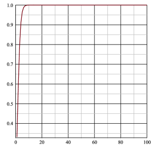
Figure 1. Proportion of closed terms in $\mathcal{L}_{N,0}$ for $N$ from 1 to 100

For this purpose, let us determine the proportion of closed lambda terms of size $n$ in the class $\mathcal{L}_{N,0}$. This proportion is just $\dfrac{[z^{n}]L_{0}(z)}{[z^{n}]L_{N,0}(z)}$. But we know that $L_{N,0}(z)$ has the same radius of convergence as $L_{0}(z)$ and that the sequence converges uniformly to $L_{0}(z)$. Even a more precise result holds, which can be seen by inspecting the system (27).

Proposition 2.

For $m=0,1,\dots,N$ there are positive constants $a_{N,m}$ and $b_{N,m}$ such that $L_{N,m}(z)\sim a_{N,m}-b_{N,m}\sqrt{1-\frac{z}{\rho}}$, as $z\to\rho$ in such a way that $\arg(z-\rho)\neq 0$.

Proof.

The last equation of (27) is the quadratic equation for $L_{N,N}(z)=L_{\infty}(z)$. Solving it yields the explicit solution for $L_{N,N}(z)$ and gives in particular

$$L_{N,N}=\frac{1-z-\sqrt{\frac{1-3z-z^{2}-z^{3}}{1-z}}}{2z}\sim a_{N,N}-b_{N,N}\sqrt{1-\frac{z}{\rho}}$$

with $\rho$ being the smallest positive root of $1-3z-z^{2}-z^{3}$ and

$$a_{N,N}=\frac{1-2\rho}{2\rho}\qquad b_{N,N}=\frac{\sqrt{3-6\rho-\rho^{2}}}{2\rho\sqrt{1-\rho}}.$$

Using the other equations of (27), solving successively from bottom up, we obtain nothing but solutions of quadratic equations. Inserting the singular expansions one after another we obtain a system of two recurrence relations for $a_{N,m}$ and $b_{N,m}$:

$$a_{N,m} =\frac{1-\sqrt{1-(1-\rho^{2})(1-\rho^{m})-4\rho^{2}a_{N,m+1}}}{2\rho},$$

$$b_{N,m} =\frac{\rho}{\sqrt{1-(1-\rho^{2})(1-\rho^{m})-4\rho^{2}a_{N,m+1}}}\cdot b_{N,m+1}.$$

From this system it is obvious that $b_{N,m}>0$ and hence all function $L_{N,m}(z)$ have indeed a singularity of type $\frac{1}{2}$. The positivity of $a_{N,m}$ is trivial, because $a_{N,m}=L_{N,m}(\rho)$, $\rho>0$ and $L_{N,m}(z)$ has positive coefficients. ∎

Now, let us return to our sampling problem and note that $\dfrac{[z^{n}]L_{0}(z)}{[z^{n}]L_{N,0}(z)}=\dfrac{b_{0}}{b_{N,0}}$. Proposition 2 gives us a procedure to compute $[z^{n}]L_{N,0}(z)$ asymptotically. The next proposition will tell us that we do not have to go very far, i.e., an $N$ of moderate size is sufficient.

Proposition 3.

The fraction $\dfrac{b_{0}}{b_{N,0}}$ tends to 1 exponentially fast, as $N$ tends to infinity.

Proof.

Consider the difference $L_{m,N}(z)-L_{m}(z)$. We have

$$L_{m,N}(z)-L_{m}(z)=z(L_{m+1,N}(z)-L_{m+1}(z))+z(L_{m,N}(z)^{2}-L_{m}(z)^{2},$$

for all $m=0,1\dots,N-1$, which implies

$$L_{m,N}(z)-L_{m}(z)=\frac{z}{1-z(L_{m,N}(z)+L_{\infty}(z))}(L_{m+1,N}(z)-L_{m+1}(z)).$$

Iterating gives

$$L_{0,N}(z)-L_{0}(z)=(L_{\infty}(z)-L_{N}(z))\prod_{\ell=0}^{N-1}\frac{z}{1-z(L_{\ell,N}(z)+L_{\ell}(z))}.$$

The function on the left-hand side has only nonnegative coefficients and therefore, in order to estimate the function it is enough to consider only positive $z$. For positive $z$ we have $L_{m,N}(z)<L_{\infty}(z)$ and $L_{m}(z)<L_{N}(z)$. Thus

$$|L_{0,N}(z)-L_{0}(z)| <|L_{\infty}(z)-L_{N}(z)|\prod_{\ell=0}^{N-1}\left|\frac{z}{1-z(L_{\infty}(z)+L_{N}(z))}\right|$$

(28) $$=|L_{\infty}(z)-L_{N}(z)|\cdot\left|\frac{z}{1-2zL_{\infty}(z)+z(L_{i}nfty(z)-L_{N}(z))}\right|^{N}.$$

By an analogous reasoning as in the proof of Lemma 5 we can derive that $|L_{\infty}(z)-L_{N}(z)|=O(N^{-1/2})$. This can be refined to $|L_{\infty}(\rho)-L_{N}(\rho)|=\Theta(N^{-1/2})$. To see this, note that as $b_{N}<b_{\infty}$, the square-root singularities of $L_{\infty}(z)$ and $L_{N}(z)$ cannot cancel when building simply the difference. Thus $L_{\infty}(z)-L_{N}(z)$ has a singularity of type $\frac{1}{2}$ as well and thus its coefficients satisfy an asymptotic of the form $\rho^{-n}n^{-3/2}$, and they are zero only for $n<N$. So, the modulus of the difference must be of order $N^{-1/2}$ when evaluated at $z=\rho$.

With this in conjunction with $1-2\rho L_{\infty}(\rho)=\rho$ the inequality (28) becomes

$$|L_{0,N}(z)-L_{0}(z)|\leq|L_{0,N}(\rho)-L_{0}(\rho)|<\frac{c_{1}}{\sqrt{N}}\left(\frac{C}{1+\frac{c_{2}}{\sqrt{N}}}\right)^{N}$$

which means that the difference $|L_{0,N}(z)-L_{0}(z)|$ is exponentially small. Likewise, $(b_{N,0}-b_{0})/b_{N,0}$ is exponentially small, because the coefficients $b_{0}$ and $b_{N,0}$ can be expressed as integrals of $L_{0,N}(z)$ and $L_{0}(z)$ by means of Cauchy’s integration formula. ∎

Obviously, our results generalize to the general case with arbitrary $a,b,c,d$ as well. Exploiting these results for the present case ($a=b=c=d=1$), shows the efficiency of the sampler: Already for $N=20$, the proportion of closed terms is 0.999999998 such that the sampler will almost never reject a drawn object.

5.4. Experiments

In this section, we deal with a Boltzmann sampler using $N=20$. It is quite interesting to analyze the behavior of this sampler. The first graphic shows the dynamic of the choice inside the system of equations. The first observation is that this dynamic tends quickly to a stable law: the probability to draw a unary node tends to 0.2955977425, the probability to draw a binary node as the probability to draw a leaf tends to 0.3522011287. In particular, this fact shows that the number of leaves in a lambda term of size $n$ is asymptotically of order $\mu n$ with $\mu\approx 0.3522011287$.

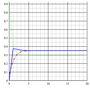
Figure 2. Example for $N=20$ of the evolution of the probability in $\Gamma L_{i}$ for $i$ from 0 to 20. The green dot line represents the probability to draw a unary node (abstraction), the red dashdot line represents the probability to draw a binary node (application), the solid blue line represents the probability to draw a leaf (variable).

Invoking the uniform convergence, we can reach more precise results on parameters. In particular, consider $X_{N}$ the random variable of the number of leaves in a uniform random term from $\mathcal{L}_{N,0}$, conditioned on the size.

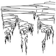
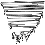
Figure 3. Three uniform random lambda terms (according to unary representation) of size respectively 2098, 2541, 2761.

First, notice that $X_{N}$ has the same distribution as the number of leaves in $\mathcal{L}_{N,N}$. This can be seen by setting up equations for the bivariate generating functions $L_{N,k}(z,u)$ where the second variable is associated to the leaves. Then, one observes that the radius of convergence $\rho_{N}(u)$ of all functions is the same and depends only on $N$. As $L_{N,0}$ converges uniformly to $L_{0}(z)$ the same applies to $\rho_{N}(u)$. Eventually, this implies that all moments of $X_{N}$ are asymptotically equal to the corresponding moments of $X$, the number of leaves in a uniform random closed term, conditioned on the size. It follows that $X$ is asymptotically Gaussian as it is the case for the number of leaves in $\mathcal{L}_{N,N}$.

Theorem 3.

Let $X_{n}$ the number of variables in a lambda term of size $n$. Then $X_{n}$ is asymptotically Gaussian with $\mathbb{E}(X_{n})\sim\alpha n$ and $\mathbb{V}ar(X)\sim\alpha n$ where $\alpha=\dfrac{1-\rho}{2}\approx 0.3522011287$.

For sampling lambda terms several approaches were use. In [36] an algorithm using memoization techniques was developed. The Haskell sampler in [26] which used recurrences for different classes of lambda terms performed better and could generate terms of size 1500 within a few hours.

Our sampler has the same complexity as the classical Boltzmann sampler for trees. In particular, it is linear in approximate size. Grygiel and Lescanne [28] already used a Boltzmann sampler using a rejection procedure based on the results presented in [24]. They were able to generate terms up to size 100 000. Our procedure refines the rejection procedure and exploits the fast convergence of the $\mathcal{L}_{N,0}$ to $\mathcal{L}_{0}$. Using a standard laptop with a CPU i7-5600U cadenced at 2.6 GHz, it is possible to draw a lambda term of size in the range [1 000 000,2 000 000]. The fairly large terms depicted in Figure 3 can be generated within a second.

References

- [1] Henk P. Barendregt. The lambda calculus. Its syntax and semantics, volume 103 of Studies in Logic and the Foundations of Mathematics. North-Holland Publishing Co., Amsterdam, revised edition, 1984.
- [2] Maciej Bendkowski, Katarzyna Grygiel, Pierre Lescanne, and Marek Zaionc. A natural counting of lambda terms. In SOFSEM 2016: theory and practice of computer science, volume 9587 of Lecture Notes in Comput. Sci., pages 183–194. Springer, Berlin, 2016.
- [3] Maciej Bendkowski, Katarzyna Grygiel, and Marek Zaionc. Asymptotic properties of combinatory logic. In Theory and applications of models of computation, volume 9076 of Lecture Notes in Comput. Sci., pages 62–72. Springer, Cham, 2015.
- [4] O. Bodini, D. Gardy, and A. Jacquot. Asymptotics and random sampling for BCI and BCK lambda terms. Theoret. Comput. Sci., 502:227–238, 2013.
- [5] Olivier Bodini, Danièle Gardy, Bernhard Gittenberger, and Zbigniew Gołębiewski. On the number of unary-binary tree-like structures with restrictions on the unary height. Annals of Combinatorics. To appear.
- [6] Olivier Bodini, Danièle Gardy, Bernhard Gittenberger, and Alice Jacquot. Enumeration of generalized lambda-terms. Electron. J. Combin., 20(4):Paper 30, 23, 2013.
- [7] Olivier Bodini, Antoine Genitrini, and Nicolas Rolin. Pointed versus singular Boltzmann samplers: a comparative analysis. Pure Math. Appl. (PU.M.A.), 25(2):115–131, 2015.
- [8] Alex Brodsky and Nicholas Pippenger. The Boolean functions computed by random Boolean formulas or how to grow the right function. Random Structures Algorithms, 27(4):490–519, 2005.
- [9] B. Chauvin, P. Flajolet, D. Gardy, and B. Gittenberger. And/or trees revisited. Combin. Probab. Comput., 13(4-5):475–497, 2004.
- [10] René David, Katarzyna Grygiel, Jakub Kozik, Christophe Raffalli, Guillaume Theyssier, and Marek Zaionc. Asymptotically almost all -terms are strongly normalizing. Log. Methods Comput. Sci., 9(1):1:02, 30 pp., 2013.
- [11] René David and Marek Zaionc. Counting proofs in propositional logic. Arch. Math. Logic, 48(2):185–199, 2009.
- [12] Veronika Daxner, Antoine Genitrini, Bernhard Gittenberger, and Cécile Mailler. The relation between tree size complexity and probability for Boolean functions generated by uniform random trees. Appl. Anal. Discrete Math., 10(2):408–446, 2016.
- [13] N. G. de Bruijn. Lambda calculus notation with nameless dummies, a tool for automatic formula manipulation, with application to the Church-Rosser theorem. Nederl. Akad. Wetensch. Proc. Ser. A 75=Indag. Math., 34:381–392, 1972.
- [14] Élie de Panafieu, Danièle Gardy, Bernhard Gittenberger, and Markus Kuba. 2-Xor revisited: satisfiability and probabilities of functions. Algorithmica, 76(4):1035–1076, 2016.
- [15] Philippe Duchon, Philippe Flajolet, Guy Louchard, and Gilles Schaeffer. Boltzmann samplers for the random generation of combinatorial structures. Combinatorics, Probability & Computing, 13(4-5):577–625, 2004.
- [16] Philippe Flajolet and Andrew M. Odlyzko. Singularity analysis of generating functions. SIAM J. Discrete Math., 3(2):216–240, 1990.
- [17] Philippe Flajolet and Robert Sedgewick. Analytic Combinatorics. Cambridge University Press, New York, NY, USA, 1 edition, 2009.
- [18] Hervé Fournier, Danièle Gardy, Antoine Genitrini, and Bernhard Gittenberger. The fraction of large random trees representing a given Boolean function in implicational logic. Random Structures Algorithms, 40(3):317–349, 2012.
- [19] Hervé Fournier, Danièle Gardy, Antoine Genitrini, and Marek Zaionc. Tautologies over implication with negative literals. MLQ Math. Log. Q., 56(4):388–396, 2010.
- [20] Danièle Gardy and Alan Woods. And/or tree probabilities of Boolean functions. In 2005 International Conference on Analysis of Algorithms, Discrete Math. Theor. Comput. Sci. Proc., AD, pages 139–146. Assoc. Discrete Math. Theor. Comput. Sci., Nancy, 2005.
- [21] Antoine Genitrini, Bernhard Gittenberger, Veronika Kraus, and Cécile Mailler. Probabilities of Boolean functions given by random implicational formulas. Electron. J. Combin., 19(2):Paper 37, 20, 2012.
- [22] Antoine Genitrini and Jakub Kozik. In the full propositional logic, 5/8 of classical tautologies are intuitionistically valid. Ann. Pure Appl. Logic, 163(7):875–887, 2012.
- [23] Antoine Genitrini and Cécile Mailler. Generalised and quotient models for random and/or trees and application to satisfiability. Algorithmica, 76(4):1106–1138, 2016.
- [24] B. Gittenberger and Z. Gołębiewski. On the number of lambda terms with prescribed size of their de bruijn representation. In 33rd Symposium on Theoretical Aspects of Computer Science (STACS), volume 40, pages 1–13, 2016.
- [25] Katarzyna Grygiel, Paweł M. Idziak, and Marek Zaionc. How big is BCI fragment of BCK logic. J. Logic Comput., 23(3):673–691, 2013.
- [26] Katarzyna Grygiel and Pierre Lescanne. Counting and generating lambda terms. Journal of Functional Programming, 23:594–628, 2013.
- [27] Katarzyna Grygiel and Pierre Lescanne. Counting terms in the binary lambda calculus. In DMTCS. 25th International Conference on Probabilistic, Combinatorial and Asymptotic Methods for the Analysis of Algorithms. Discrete Mathematics & Theoretical Computer Science, Jun 2014.
- [28] Katarzyna Grygiel and Pierre Lescanne. Counting and generating terms in the binary lambda calculus. J. Funct. Programming, 25:e24, 25, 2015.
- [29] Zofia Kostrzycka. On the density of truth of locally finite logics. J. Logic Comput., 19(6):1113–1125, 2009.
- [30] Hanno Lefmann and Petr Savický. Some typical properties of large AND/OR Boolean formulas. Random Structures Algorithms, 10(3):337–351, 1997.
- [31] Pierre Lescanne. On counting untyped lambda terms. Theoret. Comput. Sci., 474:80–97, 2013.
- [32] Helmut Prodinger. Periodic oscillations in the analysis of algorithms. Journal of the Iranian Statistical Society, 3:251–270, 2004.
- [33] Petr Savický and Alan R. Woods. The number of Boolean functions computed by formulas of a given size. In Proceedings of the Eighth International Conference “Random Structures and Algorithms” (Poznan, 1997), volume 13, pages 349–382, 1998.
- [34] John Tromp. Binary lambda calculus and combinatory logic. In Marcus Hutter, Wolfgang Merkle, and Paul M.B. Vitanyi, editors, Kolmogorov Complexity and Applications, number 06051 in Dagstuhl Seminar Proceedings, Dagstuhl, Germany, 2006. Internationales Begegnungs- und Forschungszentrum für Informatik (IBFI), Schloss Dagstuhl, Germany.
- [35] Tim van de Brug, Wouter Kager, and Ronald Meester. The asymptotics of group Russian roulette. Markov Processes and Related Fields 23 35-66 (2017), 23:35–66, 2017.
- [36] Jue Wang. Generating random lambda calculus terms. 2005. Unpublished manuscript.
- [37] Peter Winkler. Mathematical puzzles: a connoisseur’s collection. A K Peters, Ltd., Natick, MA, 2004.
- [38] Alan R. Woods. Coloring rules for finite trees, and probabilities of monadic second order sentences. Random Structures Algorithms, 10(4):453–485, 1997.
- [39] Alan R. Woods. Counting finite models. J. Symbolic Logic, 62(3):925–949, 1997.