Relativistic protons in the Coma galaxy cluster: first gamma-ray constraints ever on turbulent reacceleration

Abstract

The Fermi-LAT collaboration recently published deep upper limits to the gamma-ray emission of the Coma cluster, a cluster that exhibits non-thermal activity and that hosts the prototype of giant radio halos. In this paper we extend previous studies and use a general formalism that combines particle reacceleration by turbulence and the generation of secondary particles in the intracluster medium to constrain relativistic protons and their role for the origin of the radio halo. Our findings significantly strengthen the conclusions of previous studies and clearly disfavour pure secondary models for the halo. Indeed the new limits allow us to conclude that a pure hadronic origin of the radio halo would require magnetic fields that are too strong. For instance $B_{0}>21\mu$G is found in the cluster center assuming that the magnetic energy density scales with thermal density, to be compared with $B_{0}\sim 4-5\mu$G as inferred from Faraday Rotation Measures (RM) under the same assumption. Secondary particles can still generate the observed emission if they are reaccelerated. For the first time the deep gamma-ray limits allow us to derive meaningful constraints if the halo is generated during phases of reacceleration of relativistic protons and their secondaries by cluster-scale turbulence. In this paper we explore a limited, but relevant, range of parameter-space of reacceleration models. Within this parameter space a fraction of model configurations is already ruled out by current gamma-ray limits, including the cases that assume weak magnetic fields in the cluster core, $B\leq 2-3\mu$G. Interestingly, we also find that the flux predicted by a large fraction of model configurations that assume a magnetic field consistent with Faraday RM is not far from the limits. This suggests that a detection of cosmic-ray-induced gamma rays from the cluster might be possible in the near future, provided that the electrons generating the radio halo are secondaries reaccelerated and the magnetic field in the cluster is consistent with that inferred from Faraday RM.

1 Introduction

Clusters of galaxies form during the most violent events known in the Universe by merging and accretion of smaller structures onto larger ones (see Voit, 2005, for a review). This process is accompanied by a release of energy of the order of the cluster gravitational binding energy of about $10^{62}-10^{64}$ erg. Some of this energy is dissipated via shock waves and turbulence through the intra-cluster medium (ICM) that can (re-)accelerate particles to relativistic energies (see, e.g. Brunetti & Jones, 2014, for a review). In fact, the presence of relativistic electrons in the ICM, as well as $\mu$G magnetic fields, is probed by the detection of diffuse cluster-scale synchrotron radio emission in several clusters of galaxies. Mpc-scale diffuse synchrotron emission in clusters is classified in two main categories: radio halos, roundish radio sources located in the central regions, and radio relics, filamentary structures tracing shock waves in the cluster outskirts (Feretti et al., 2012, for a review) The origin of these synchrotron sources has been debated for decades now and, while some important steps have been made, important ingredients in the scenario for the origin of non-thermal phenomena in clusters remain poorly understood (Brunetti & Jones, 2014, for a review).

Giant radio halos are the most spectacular evidence for non-thermal phenomena in galaxy clusters. The short cooling length of relativistic electrons at synchrotron frequencies compared to the scale of these sources requires mechanisms of in situ acceleration or injection of the emitting particles. Cosmic-ray (CR) protons are accelerated by structure formation shocks and galaxy outflows in clusters, they can accumulate and are confined there for cosmological times and, therefore, can diffuse on Mpc volumes (e.g., Völk et al., 1996; Berezinsky et al., 1997) For these reasons, a natural explanation for radio halos was given by the so-called hadronic model (pure secondary model throughout this paper; e.g., Dennison, 1980; Blasi & Colafrancesco, 1999; Pfrommer & Enßlin, 2004; Pfrommer et al., 2008; Pinzke & Pfrommer, 2010; Keshet & Loeb, 2010; Enßlin et al., 2011). In this scenario the observed diffuse radio emission in cluster central regions is explained by secondary electrons that are continuously generated by inelastic collisions between CR protons and thermal protons of the ICM. However the same inelastic collisions generate also gamma rays (from $\pi^{0}$ decay) whose non detection in these years (e.g., Aharonian et al., 2009a, b; Aleksić et al., 2010, 2012; Arlen et al., 2012; Ackermann et al., 2010; Huber et al, 2013; Prokhorov & Churazov, 2014; Ahnen et al., 2016) limits the cluster CR content and in fact disfavors a pure hadronic origin of radio halos (e.g., Brunetti et al., 2009; Jeltema & Profumo, 2011; Brunetti et al., 2012; Zandanel et al., 2014; Zandanel & Ando, 2014; Ackermann et al., 2014, 2016). While there are other complementary evidences that put tension on pure hadronic models, for example as inferred from cluster radio–thermal scaling relations and spectrum of radio halos (Brunetti & Jones, 2014, for review), gamma-ray (and also neutrino; e.g., Berezinsky et al., 1997; Zandanel et al., 2015) observations are the only direct ways of constraining CRs in clusters.

Nowadays, the favored explanation for giant radio halos is given by the so-called turbulent re-acceleration model, where particles are re-accelerated to emitting energies by turbulence generated during cluster mergers (Brunetti et al., 2001; Petrosian, 2001; Fujita et al., 2003; Cassano & Brunetti, 2005; Brunetti & Lazarian, 2007; Donnert et al., 2013; Beresnyak et al., 2013; Miniati, 2015; Brunetti & Lazarian, 2016; Pinzke et al., 2017; Eckert et al., 2017); a scenario that requires a complex hierarchy of mechanisms and plasma collisionless effects operating in the ICM. This scenario has the potential to fit well with a number of observations: from the radio halo – merger connection, to spectral and spatial characteristics of the diffuse synchrotron emission. However, one of the critical points in this scenario is the need of seed (relativistic) electrons for the re-acceleration (e.g., Petrosian & East, 2008). A natural solution for this problem is again to assume that these seeds are secondary electrons coming from CR-ICM hadronic collisions (Brunetti & Blasi, 2005; Brunetti & Lazarian, 2011; Pinzke et al., 2017). In this case, while the CR-proton content needed to explain radio halos is lower than in the pure hadronic scenario, one also expects some level of gamma-ray emission. Being able to test this level of emission would allow to constrain the role of hadrons for the origin of the observed non-thermal emission in galaxy clusters and also to constrain fundamental physical parameters of the turbulence and of the acceleration and diffusion of relativistic particles in the ICM.

The Coma cluster of galaxies hosts the best studied prototype of a giant radio halo (Wilson, 1970; Giovannini et al., 1993). In this work we use the latest observations of the Coma cluster by the Large Area Telescope (LAT) on board of the Fermi satellite - in particular the publicly available likelihood curves (Ackermann et al., 2016) - to constrain the role of CRp for the origin of the halo, significantly extending previous studies by Brunetti et al. (2012), Zandanel & Ando (2014) and Pinzke et al. (2017). Specifically we test a scenario based on pure hadronic models, and a more complex scenario based on turbulent re-acceleration of secondary particles. We use the surface brightness profile of the Coma giant radio halo as measured by Brown & Rudnick (2011) at 350 MHz and the synchrotron radio spectrum of the halo as priors for the modeling of the gamma-ray emission. The magnetic field is a very important ingredient in the modeling as the ratio between gamma rays and the observed radio emission depends on the field strength and spatial distribution in the cluster. We assume the magnetic field as free parameter while noting that Faraday Rotation Measures (RM) are available for Coma (Bonafede et al., 2010), and we take these to be our baseline model. We will show that we are now able to exclude a pure hadronic origin of the diffuse radio emission, unless extremely high magnetic fields - in clear contrast with RM - are assumed, therefore, extending previous works in the same direction (Brunetti et al., 2012; Zandanel et al., 2014; Zandanel & Ando, 2014). More importantly, we show for the first time that gamma-ray observations by Fermi-LAT allow now to start testing the turbulent re-acceleration scenario for the Coma giant radio halo, thereby opening up a new window into the study of non-thermal phenomena in clusters with high-energy observations. Interestingly, Selig et al. (2015) performed a re-analysis of the Fermi-LAT data with an approach based on information theory and found significant emission toward the direction of several galaxy clusters. However, due to the limitations of their analysis, it remains to be seen if these signals indeed belong to clusters or to point-sources. On a similar note, recently, Branchini et al. (2017) reported the detection of cross-correlation between the Fermi-LAT data and several galaxy cluster catalogues. Also in this case it was not possible to disentangle between truly ICM-related diffuse emission and point-sources. Nevertheless, these two works, together with the conclusions of our paper, may point to a brighter future for gamma-ray observations of clusters.

This paper is organised as follows. In Sections 2 and 3, we introduce the physical scenario and the formalism adopted for our calculations. In Section 4, we explain the method used to obtain Fermi-LAT limits and the constrains on the combined magnetic and CR properties from radio observations. We discuss our results on both pure hadronic and the general re-acceleration scenarios in Section 5, and provide a discussion including the main limitations of the work in Section 6. Conclusions are given in Sction 7.

In this paper we assume a $\Lambda$CDM cosmology with $H_{0}=70$km s^-1 Mpc^-1, $\Omega_{\Lambda}=0.7$ and $\Omega_{m}=0.3$.

2 The physical scenario

In this paper we explore the general scenario where CRp and their secondaries are reaccelerated by ICM turbulence. This scenario has the potential to explain giant radio halos depending on the combination of turbulent-acceleraion rate and injection rate of secondary particles (e.g., Brunetti & Lazarian, 2011; Pinzke et al., 2017). In addition, this scenario also produces gamma rays. However, as turbulence in the ICM cannot reaccelerate electrons to TeV energies, the gamma-ray emission is powered only by the process of continuous injection of secondary particles due to proton-proton collisions in the ICM ($\pi^{0}$-decay and inverse Compton (IC) from TeV secondary electrons) and ultimately depends on the energy budget in the form of CRp in the ICM at the epoch of observation.

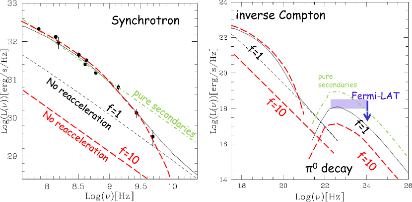
Figure 1: An example of typical radio (left) and high-energy (right) spectrum predicted by reacceleration models that consider both primary and secondary particles. The example is that of a Coma–like cluster assuming a configuration of the magnetic field from Faraday RM and a reacceleration rate that is suitable to match the steepening of the radio spectrum, $\tau_{\mathrm{acc}}\sim 300$ Myr. The cases $f=1$ (black) and $=10$ (red) are shown in the case of reacceleration and normalised to the radio spectrum (i.e. with CRp number tuned to match the radio spectrum during reacceleration). The non-thermal emission from the two models assuming $\tau_{acc}^{-1}=0$ (no reacceleration, i.e. after turbulence is dissipated) is also shown for comparison, note that in this case the non-thermal luminosity scales about with $f^{-1}$. The case of a pure secondary model anchored to the observed radio emission at 1.4 GHz is also shown (green) together with the coresponding gamma-ray spectrum that is expected due to $\pi^{0}$ decay.

For sake of clarity, in this Section we will briefly review the expectations and main dependencies of the scenario. Calculations of (merger-induced) turbulent reacceleration of primary and secondary particles predict a complex spectral energy distribution (SED) of the non-thermal radiation that extends from radio to gamma rays. The SED is made of several components that have different evolutions in time; an example for the Coma cluster is given in Figure 1.

In dynamically disturbed (merger) and turbulent systems, models predict a transient component of the SED that is generated by turbulent acceleration in the ICM. This transient component is expected to have a typical time-scale of about 1-3 Gyr. During mergers particle acceleration by turbulence boosts up the synchrotron and IC emission making the cluster-scale non-thermal emission more luminous in the radio and hard X-ray bands (Fig. 1). In fact the observed giant radio halos seems to be generated during this transient phase (Brunetti & Jones, 2014, for a review). The strength and spectral properties of the transient component of the SED depend on the acceleration parameters and physical conditions in the ICM.

In addition to the transient component, long living radio, IC and gamma-ray emission, sustained by the continuous injection of high energy secondary CRe and by the decay of neutral pions, is expected to be common in clusters (Fig. 1). The strength of this persistent component is proportional to the energy density of the primary CRp and depends on their spatial distribution in the ICM. Long living synchrotron emission can generate under-luminous/off-state radio halos that may become visible in future radio surveys (e.g., Brown et al, 2011; Cassano et al, 2012).

The relative strength of the transient and longer living component of the SED depends on the efficiency of particle acceleration and energy losses in the ICM. Furthermore, in general, this also depends on the ratio of primary and secondary electrons that become available to the reacceleration process. The ratio between the two populations is poorly known. Primary relativistic electrons can be accumulated and maintained in galaxy clusters at energies of about 100 MeV (Brunetti & Jones, 2014, for a review), so they may provide a suitable population of seeds to reaccelerate (e.g. Brunetti et al., 2001; Cassano & Brunetti, 2005; Pinzke et al., 2013; Pinzke et al., 2017). For this reason it is convenient to define a parameter $f=1+{{N_{e,pr}}\over{N_{e^{\pm}}}}$, where $N_{e,pr}/N_{e^{\pm}}$ is the ratio of primary and secondary electrons that become available for reacceleration; $f=1$ is the case where only CR protons (and their secondaries) are present in the ICM. In Fig. 1 we show the differences in the SED that are caused by different assumptions for the ratio between primary and secondary electrons, $f=1$ and 10 respectively. Once the radio data points are used to constrain the amount of reaccelerated electrons (other model parameters being fixed), the gamma-ray luminosity declines with increasing $f$. This is essentially because less secondaries, and less CRp, are assumed in the model in order for it to match the radio data.

If turbulent reacceleration does not play a role the scenario is that of a pure secondary model where the spectrum of electrons and the SED are simply governed by the injection of secondary particles due to CRp-p collisions and by the radiative electron energy losses. Pure hadronic models have also been proposed for the origin of giant radio halos (Dennison, 1980; Blasi & Colafrancesco, 1999; Pfrommer & Enßlin, 2004; Keshet & Loeb, 2010). However, in the last decade radio observations and their combination with complementary constraints in the X-ray and gamma-ray bands have put significant tension on this scenario (Brunetti & Jones, 2014, for a review). One reason for this tension originates from the non detection of galaxy clusters in gamma rays as discussed in the Introduction. This is shown in Figure 1 (green lines): the CRp energy budget that is necessary to match the synchrotron flux of the radio halo is much larger than that in the reacceleration models (other model parameters being the same) with the consequence to generate gamma rays in excess of observed limits from gamma-ray observatories, both space-borne and ground-based. To circumvent this problem a larger value of the magnetic field must be assumed in the ICM. However it has been shown, for a number of nearby clusters, that the magnetic field required to explain radio halos without generating too many gamma rays is larger or in tension with independent estimates based on Faraday rotation measures alone (e.g., Jeltema & Profumo, 2011; Brunetti et al., 2012) (see also Sect. 5.1).

3 Formalism adopted in the paper

The aim of this Section is to present the essential information about the formalism and the main assumptions used in our calculations.

3.1 Time evolution of particles spectra

We model the time evolution of the spectral energy distribution of electrons, $N_{e}^{-}$, and positrons, $N_{e}^{+}$, with standard isotropic Fokker-Planck equations:

$${{\partial N_{e}^{\pm}(p,t)}\over{\partial t}}={{\partial}\over{\partial p}}\Big{[}N_{e}^{\pm}(p,t)\Big{(}\left|{{dp}\over{dt}}\right|_{\rm rad}-{1\over{p^{2}}}{{\partial}\over{\partial p}}(p^{2}D_{\rm pp}^{\pm})$$

$$+\left|{{dp}\over{dt}}\right|_{\rm i}\Big{)}\Big{]}+{{\partial^{2}}\over{\partial p^{2}}}\left[D_{\rm pp}^{\pm}N_{e}^{\pm}(p,t)\right]$$

$$+Q_{e}^{\pm}[p,t;N_{p}(p,t)]\,,$$ (1)

where $|dp/dt|$ marks radiative (r) and Coulomb (i) losses (Sect. 3.2), $D_{pp}$ is the electron/positron diffusion coefficient in the particles momentum space due to the coupling with turbulent fluctuations (Sect. 3.3), and the term $Q_{e}^{\pm}$ accounts for the injection rate of secondary electrons and positrons due to p-p collisions in the ICM (Sect. 3.4).

Similarly, the time evolution of the spectral energy distribution of protons, $N_{p}$, is given by:

$${{\partial N_{p}(p,t)}\over{\partial t}}={{\partial}\over{\partial p}}\Big{[}N_{p}(p,t)\Big{(}\left|{{dp}\over{dt}}\right|_{\rm i}-{1\over{p^{2}}}{{\partial}\over{\partial p}}(p^{2}D_{\rm pp})\Big{)}\Big{]}$$

$$+{{\partial^{2}}\over{\partial p^{2}}}\left[D_{\rm pp}N_{p}(p,t)\right]-{{N_{p}(p,t)}\over{\tau_{pp}(p)}}+Q_{p}(p,t)\,,$$ (2)

where $|dp/dt_{i}|$ marks Coulomb losses (Sect. 3.2), $D_{pp}$ is the diffusion coefficient in the momentum space of protons due to the coupling with turbulent modes (Sect. 3.3), $\tau_{pp}$ is the proton lifetime due to p-p collisions in the ICM (Sect. 3.4), and $Q_{p}$ is a source term.

In our modelling the Fokker-Planck equations for protons, electrons and positrons are coupled with an equation that describes the time evolution of the spectrum of turbulence, ${\cal W}(k,t)$. For isotropic turbulence (see Sect. 3.3) the diffusion equation in the k–space of the modes is given by:

$${{\partial{\cal W}(k,t)}\over{\partial t}}={{\partial}\over{\partial k}}\left(k^{2}D_{kk}{{\partial}\over{\partial k}}({{{\cal W}(k,t)}\over{k^{2}}})\right)+I(k,t)$$

$$-\sum_{i}\Gamma_{i}(k,t){\cal W}(k,t)\,\,\,,$$ (3)

where the relevant coefficients are the diffusion coefficient in the k–space, $D_{kk}$, the combination of the relevant damping terms, $\Gamma_{i}(k,t)$, and the turbulence injection/driving term, $I(k,t)$ (see Sect. 3.3).

The four differential equations provide a fully coupled system: the particle reacceleration rate is determined by the turbulent properties, these properties are affected by the turbulent damping due to the same relativistic (and thermal) particles, and the injection rate and spectrum of secondary electrons and positrons is determined by the proton spectrum which (also) evolves with time.

3.2 Energy losses for electrons and protons

The energy losses of relativistic electrons in the ICM are dominated by ionization and Coulomb losses, at low energies ($\leq$100-300 Myr), and by synchrotron and IC losses, at higher energies (Brunetti & Jones, 2014, for a review).

The rate of Coulomb losses for electrons is dominated by the effect of CRe-e collisions in the ICM. For ultrarelativistic electrons the losses can be approximated as (in cgs units):

$$\left|{{dp}\over{dt}}\right|_{\rm i}\simeq 3.3\times 10^{-29}n_{\rm th}\left[1+{{{\rm ln}((p/mc)/{n_{\rm th}})}\over{75}}\right]$$ (4)

where $n_{\rm th}$ is the number density of the thermal plasma. The rate of synchrotron and IC losses is (in cgs units):

$$\left|{{dp}\over{dt}}\right|_{\rm rad}\simeq 4.8\times 10^{-4}p^{2}\left[\left({{B_{\mu G}}\over{3.2}}\right)^{2}+(1+z)^{4}\right]$$ (5)

where $B_{\mu G}$ is the magnetic field strength in units of $\mu G$. Eqs.4–5 provide the coefficients in Eq. 1.

For ultra-relativistic protons, in the energy range 10 GeV – 100 TeV, the main channel of energy losses in the ICM is provided by inelastic CRp-p collisions. The lifetime of protons (in Eq.  2) due to CRp-p collisions is given by:

$$\tau_{pp}(p)={1\over{c\,n_{th}\sigma_{in}}}$$ (6)

where $\sigma_{in}$ is the total inelastic cross section. In this paper we use the parameterization for the inelastic cross section given by Kamae et al. (2006, 2007) combining the contributions from the non-diffractive, diffractive and resonant-excitation ($\Delta(1232)$ and res(1600)) parts of the cross section.

In our calculations it is important also to follow correctly the evolution (acceleration and losses) of supra-thermal, trans-relativistic and mildly relativistic protons. Indeed during reacceleration phases these particles might be reaccelerated and contribute significantly to the injection of secondary particles. At these energies the particle energy losses are dominated by Coulomb collisions due to CRp-p and CRp-e interactions. Following Petrosian & Kang (2015) the energy losses due to the combined effect of CRp-p and CRp-e Coulomb interactions is (in cgs units):

$$\left|{{dp}\over{dt}}\right|_{i}\simeq 3.8\times 10^{-29}n_{th}\left(1-{{k_{B}T/(2m_{p}c^{2})}\over{\sqrt{1+(p/(m_{p}c))^{2}}-1}}\right)$$

$$\times\big{(}{{\ln\Lambda}\over{38}}\big{)}\sum_{j=e,p}\left(\int_{0}^{\sqrt{x_{j}}}\exp{(-y^{2})}dy-\sqrt{x_{j}}\exp{(-x_{j})}\right)$$ (7)

where $\Lambda$ is the Coulomb logarithm, and $x_{j}=(E_{p}/k_{B}T)(m_{j}/m_{p})$, $j=e,p$ is for p-e and p-p interactions, respectively. Eq. 7 provides the coefficient for energy losses in Eq. 2.

3.3 Turbulence and particle acceleration

Particle acceleration in the ICM has been investigated in numerous papers (Schlickeiser et al., 1987; Brunetti et al., 2001, 2004; Petrosian, 2001; Fujita et al., 2003, 2015; Cassano & Brunetti, 2005; Beresnyak et al., 2013; Brunetti & Lazarian, 2016), with particular focus on the effect of compressive turbulence induced during cluster mergers (Brunetti & Lazarian, 2007, 2011; Miniati, 2015; Brunetti, 2016; Pinzke et al., 2017). A commonly adopted mechanism is the Transit-Time-Damping (TTD) (Fisk, 1976; Eilek, 1979; Miller et al., 1996; Schlickeiser & Miller, 1998) with fast modes. This mechanism is essentially driven by the resonance between the magnetic moment of particles and the magnetic field gradients parallel to the field lines. The mechanism induces a random walk in the particle momentum space with diffusion coefficient $D_{pp}$ (Appendix A):

$$D_{pp}\simeq{{\pi^{2}}\over{2c}}{{c_{s}^{2}}\over{B_{0}^{2}}}{{p^{2}}\over{\beta}}\int_{{c_{s}}\over{\beta c}}^{1}{\cal H}(1-{{c_{s}}\over{\beta c}}){{1-\mu^{2}}\over{\mu}}d\mu\left[1-\big{(}{{c_{s}}\over{\mu\beta c}}\big{)}^{2}\right]^{2}$$

$$\times\int_{k_{0}}^{k_{cut}}dkkW_{B}$$ (8)

where $\mu$ is the cosine of the particle pitch angle, $W_{B}$ is the spectrum of turbulent magnetic fluctuations, $k_{0}$ and $k_{cut}$ are the injection and cut-off wavenumbers respectively, and ${\cal H}$ is the Heaviside function. Eq. 8 provides the diffusion coefficient in the particles momentum space that is used in Eqs.1–2. For ultra-relativistic particles the resulting particles acceleration time, $\tau_{\mathrm{acc}}=p^{2}/(4D_{pp})$, is independent from the particle momentum.

More specifically in this paper we obtain the spectrum of magnetic turbulence in Eq. 8, $W_{B}$, from Eq. 3 assuming $|B_{k}|^{2}\sim 16\pi\beta_{\mathrm{pl}}W$ (see Brunetti & Lazarian, 2007), $\beta_{\mathrm{pl}}$ is the plasma beta. In first approximation, this spectrum is expected to be a power-law induced by wave-wave cascade down to a cut-off scale, $k_{cut}$, where the turbulent-cascading time becomes comparable to or longer than the damping time, $\Gamma^{-1}$. The cut-off scale and the amount of turbulent energy (electric$/$magnetic field fluctuations) that is associated with the scales near the cut-off scale set the rate of acceleration. In this paper we adopt a Kraichnan treatment to describe the wave-wave cascading of compressible MHD waves; this gives (see, e.g., Brunetti, 2016):

$$k_{cut}\simeq{{81}\over{4}}\left({{\delta V^{2}}\over{c_{s}}}\right)^{2}{{k_{o}}\over{(\sum_{\alpha}\langle\Gamma_{\alpha}\rangle k^{-1})^{2}}}$$ (9)

where the velocity of large-scale eddies is $\delta V\sim\sqrt{W(k_{o})k_{o}}$, $k_{0}^{-1}$ is the injection scale and $<..>$ marks pitch-angle averaging. The damping rate $\sum\langle\Gamma\rangle$ in Eq. 9 is contributed also by the collisionless coupling with the relativistic particles (Brunetti & Lazarian, 2007; Brunetti, 2016) and consequently the cut-off scale, acceleration rate and the spectrum of particles are derived self-consistently from the solution of the four coupled equations in Sect. 3.1. Two scenarios can be considered to estimate the damping of fast modes in the ICM (e.g., Brunetti, 2016). (i) One possibility is that the interaction between turbulent modes with both thermal and CRs is fully collisionless. This happens when the collision frequency between particles in the ICM is $\omega_{ii}<\omega=kc_{s}$; for example this is the case where ion-ion collisions in the thermal ICM are due to Coulomb collisions. (ii) The other possibility is that only the interaction between turbulence and CRs is collisionless. This scenario is motivated by the fact that the ICM is a weakly collisional high-beta plasma that is unstable to several instabilities that can increase the collision frequencies in the thermal plasma and induce a collective interaction of individual ions with the rest of the plasma (see e.g., Schekochihin & Cowley, 2006; Brunetti & Lazarian, 2011b; Santos-Lima, et al., 2014; Kunz, et al., 2014; Santos-Lima, et al., 2017). In this paper we adopt the most conservative scenario that is based on a fully collisionless interaction between turbulence and both thermal particles and CRs (case i). In this case the damping of compressive modes is dominated by TTD with thermal particles (Brunetti & Lazarian, 2007) which also allows to greatly reduce the degree of coupling between Eqs. 1–3 and to simplify calculations. For large beta-plasma, $\beta_{\mathrm{pl}}$, the dominant damping rate is due to thermal electrons $\Gamma_{e}\sim c_{s}k\sqrt{3\pi(m_{e}/m_{p})/20\mu^{2}}\exp(-5(m_{e}/m_{p})/3\mu^{2})(1-\mu^{2})$, leading to (from Eq. 9) $k_{cut}\sim 10^{4}k_{0}M_{0}^{4}$, where $M_{0}=\delta V/c_{s}$ is the turbulent Mach number.

3.4 Injection of Secondary Electrons

The decay chain that we consider for the injection of secondary particles due to CRp-p collisions in Eq. 1 is (e.g. Blasi & Colafrancesco, 1999):

$$p+p\to\pi^{0}+\pi^{+}+\pi^{-}+\rm{anything}$$

$$\pi^{0}\to\gamma\gamma$$

$$\pi^{\pm}\to\mu^{\pm}+\nu_{\mu}(\bar{\nu}_{\mu})\,\,\,\,\,,\,\,\,\,\,\mu^{\pm}\to e^{\pm}+\bar{\nu}_{\mu}({\nu}_{\mu})+\nu_{e}(\bar{\nu}_{e}).$$

that is a threshold reaction that requires CRp with kinetic energy larger than $T_{p}\approx 300$ MeV. The injection rate of charged and neutral pions is given by:

$$Q_{\pi}^{\pm,0}(E,t)=n_{th}c\int_{p_{*}}dpN_{p}(p,t)\beta_{p}{{d\sigma^{\pm,0}}\over{dE}}(E_{\pi},E_{p})$$ (10)

where $d\sigma^{\pm,0}/dE$ is the differential inclusive cross section for the production of charged and neutral pions. A practical and useful approach that we adopt in this paper to describe the pion spectrum both in the high energy and low energy regimes is based on the combination of the isobaric and scaling model (Dermer, 1986; Moskalenko & Strong, 1998). Specifically, in this paper we consider four energy ranges to obtain a precise description of the differential cross section from low to high energies:

• for $E_{p}\leq 3$ GeV we use the isobaric model, specifically we use Eqs. 23-28 in Brunetti & Blasi (2005);

• for $3\leq E_{p}/{\mathrm{GeV}}\leq 7$, we use a combination of the isobaric model with the parametrization given in Blattnig et al. (2000), specifically their Eqs.24,26,28;

• for $7\leq E_{p}/{\mathrm{GeV}}\leq 40$, we use a combination of the aforementioned Blattnig-parametrization and the scaling model from Kelner et al. (2006) based on QGSJET simulations, Eqs. 6–8;

• finally, for $E_{p}>40$ GeV we use the aforementioned scaling model.

The decay of $\pi^{0}$–decay generates gamma rays with spectrum:

$$Q_{\gamma}(E_{\gamma},t)=2\int_{E_{min}}^{E_{p,max}}{{Q_{\pi}^{0}(E_{\pi},t)}\over{\sqrt{E_{\pi}^{2}-m_{\pi}^{2}c^{4}}}}dE_{\pi}$$ (11)

where $E_{min}=E_{\gamma}+m_{\pi}^{2}c^{4}/(4E_{\gamma})$. The injection rate of relativistic electrons/positrons is given by:

$$Q^{\pm}_{e}(p,t)=c\int_{E_{\pi}}Q^{\pm}_{\pi}(E_{\pi^{\pm}},t)dE_{\pi}\int dE_{\mu}\times$$

$$F_{e^{\pm}}(E_{\pi},E_{\mu},E_{e})F_{\mu}(E_{\mu},E_{\pi}),$$ (12)

where $F_{e}^{\pm}(E_{e},E_{\mu},E_{\pi})$ is the spectrum of electrons and positrons from the decay of a muon of energy $E_{\mu}$ produced in the decay of a pion with energy $E_{\pi}$, and $F_{\mu}(E_{\mu},E_{\pi})$ is the muon spectrum generated by the decay of a pion of energy $E_{\pi}$. In this paper we follow the approach in Brunetti & Blasi (2005) to calculate Eq. 12, in this case the injection rate of secondary electrons and positrons is:

$$Q^{\pm}_{e}(p,t)={{8\beta_{\mu}^{\prime}m_{\pi}^{2}n_{th}c^{2}}\over{m_{\pi}^{2}-m_{\mu}^{2}}}\int_{E_{\rm min}}\int_{p_{*}}{{dE_{\pi}dp}\over{E_{\pi}{\bar{\beta}}_{\mu}}}\beta_{p}N_{p}(p,t)$$

$$\times{{d\sigma^{\pm}}\over{dE}}(E_{\pi},E_{p})F_{e}(E_{e},E_{\pi})\,,$$ (13)

where $F_{e}(E_{e},E_{\pi})$ is given in Brunetti & Blasi (2005) (their Eqs. 36-37), ${\bar{\beta}}_{\mu}=\sqrt{1-m_{\mu}^{2}/\bar{E}_{\mu}^{2}}$, ${\bar{E}_{\mu}}=1/2E_{\pi}(m_{\pi}^{2}-m_{\mu}^{2})/(\beta_{\mu}^{\prime}m_{\pi}^{2})$, and $\beta_{\mu}^{\prime}\simeq 0.2714$. Eq.  13 is the injection spectrum used in Eq.  1.

3.5 A note on pure hadronic models

If turbulence is not present (or negligible acceleration) our formalism describes a pure hadronic model where the spectrum of electrons is simply determined by the balance between the injection rate due to CRp-p collisions and the cooling due to radiative and Coulomb losses.

Under these conditions, if the proton spectrum evolves slowly (on time-scales that are much longer than those of electron radiative and Coulomb losses) after a few electron cooling times, the spectrum of electrons reaches quasi-stationary conditions. From Eq. 1, with $\partial N/\partial t=0$ and $D_{pp}=0$, one then has (e.g., Dolag & Ensslin, 2000):

$$N_{e}^{\pm}(p;t)={1\over{\sum_{r,i}\big{|}{{dp}\over{dt}}\big{|}}}\int_{p}Q^{\pm}_{e}(p;t)pdt\,.$$ (14)

We note indeed that the timescale of CRp-p collisions of relativistic protons in the ICM is much longer than the radiative (and Coulomb) lifetime of GeV electrons (see, e.g. Blasi et al., 2007; Brunetti & Jones, 2014, for reviews), and consequently the use of Eq. 14 is fully justified to model the spectrum of radio-emitting electrons.

4 Method

The main goal of this paper is to constrain the role of relativistic protons for the origin of the observed radio emission in the Coma cluster. To do that we model the observed spectrum and brightness distribution of the Coma radio halo assuming different CR scenarios and compare the expected gamma-ray emission with the upper limits derived from the Fermi-LAT.

4.1 Constraints from the radio emission

The recent WSRT observations of the Coma halo at 350 MHz (Brown & Rudnick, 2011) have reached an unprecedented sensitivity to low surface brightness emission on large scales and allowed to derive solid measurements of the brightness of the halo up to large, $\sim 1$ Mpc, distance from the center (Brunetti et al., 2012, 2013; Ade et al., 2013; Zandanel & Ando, 2014). In Figure 2 we show the integrated flux of the Coma halo at 350 MHz as a function of distance.This figure shows that the halo is clearly detected up to 1 Mpc distance from the center and that the majority of the emission of the halo is produced in the range of distances 0.4-1.0 Mpc. We note that the profile derived from these WSRT observations is consistent with other profiles at 330 MHz (Govoni et al., 2001) and 140 MHz (Pizzo, 2010), at least within the aperture radius where these oldest observations are sensitive enough. On the other hand it is inconsistent with the profile obtained by Deiss et al (1997) using Effelsberg observations at 1.4 GHz, possibly suggesting systematics or flux calibration errors in the observations at 1.4 GHz (see eg., Pinzke et al., 2017).

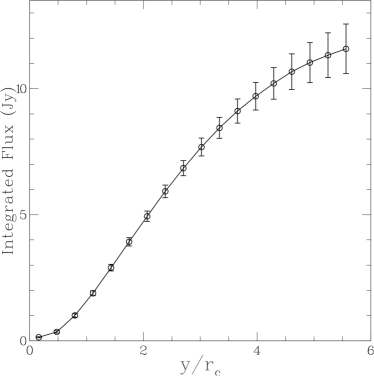
Figure 2: The radio flux of the Coma cluster measured at 325 MHz as a function of the projected radial distance (in unit of core radius; $R_{500}\simeq 5r_{c}$). Note that the integrated profile is obtained excluding the quadrant containing NGC 4869 and multiplying by $4/3$ the flux measured within the three quadrants (see Brunetti et al., 2013 for details).

If the radio halo is due to secondary particles, the observed profile constrains spatial distribution and energy density of CRp for a given configuration of the magnetic field and model of the CRp spectrum. The additional needed ingredient is the the spatial distribution of the thermal target protons obtained from the X-ray observations; we adopt the beta-model profile derived from ROSAT PSPC observations (Briel et al., 1992) with $r_{c}=290$ kpc, $\beta=0.75$ and central density $n_{\mathrm{ICM}}(0)=3.42\times 10^{-3}$cm^-3, $r_{c}$ being the core radius of the cluster. When necessary, in order to derive the ratio of CRp to thermal energy densities, we also use the temperature profile of the Coma cluster taken from XMM and Suzaku observations (Snowden et al., 2008; Wik et al., 2009).

The magnetic field in the Coma cluster has been constrained from RM (Bonafede et al., 2010, 2013). Following these studies, in our paper we assume a scaling of the magnetic field strength with cluster thermal density in the general form:

$$B(r)=B_{0}\left({{n_{\mathrm{ICM}}(r)}\over{n_{\mathrm{ICM}}(0)}}\right)^{\eta_{B}}$$ (15)

where $B_{0}$ and $\eta_{B}$ are free parameters in our calculations. As a reference, $B_{0}=4.7\mu$G and $\eta_{B}=0.5$ provides the best fit to RM data (Bonafede et al., 2010).

In addition to the brightness profile, the other observable that we use to constrain model parameters is the spectrum of the halo that is measured across more than two decades in frequency range (Thierbach et al., 2003; Pizzo, 2010). The radio spectrum constrains the spectrum of electrons and if the halo is generated by secondary particles it can be used to put constraints on the spectrum of CRp. This link however is not straightforward. For example the spectral slope of the radio halo in reacceleration models is more sensitive to the reacceleration parameters rather than to the spectrum of the primary CRp. For this reason we will discuss the constraints from the spectrum of the halo separately in the case of pure hadronic models (Sects. 5.1) and in the general scenario (Sect. 5.2).

4.2 Gamma-ray limits from Fermi-LAT

Deriving meaningful limits to the gamma-ray luminosity and CRp energy content of the Coma cluster is not straightforward because the gamma-ray flux and its brightness distribution depend on the spatial distribution of CRp and on their spectrum. The most convenient approach is thus to generate models of CRp (spectrum and spatial distribution) that explain the radio properties of the halo, calculate the expected gamma-ray emission model (spectrum and brightness distribution), and determine if a specific cluster model is in conflict with Fermi-LAT data. While the models and results are discussed in Sect. 5.1–5.2, here we describe the general procedure that is adopted in the paper to obtain the corresponding gamma-ray limits (see also Section 6.1 for a discussion regarding the expected sensitivity of LAT observations with respect to these models).

We make use of the latest published likelihood curves in Ackermann et al. (2016) which investigated the Coma cluster using the latest data release from the Fermi Large Area Space telescope ("Pass 8"). In contrast to previous analyses (Ackermann et al., 2010; Zandanel & Ando, 2014; Ackermann et al., 2014), this analysis reported a faint residual excess, however below the threshold of claiming a detection. In addition to considering a set of baseline spatial templates, the analysis presented in Ackermann et al. (2016) also provided a set of likelihood curves per energy bin for disks of varying radii around the center of the Coma cluster ($\alpha_{2000}=194.95$, $\delta_{2000}=27.98$).

We assume that any CR-induced gamma-ray template can be modeled as disk of unknown radius $r$ (Appendix B), and devised the following approach to determine whether or not the predicted gamma-ray emission of a specific CR model is in conflict with the data presented in Ackermann et al. (2016). For a given physical model $M$, based on the radio constraints (Sect. 4.1, Sect. 5.1–5.2), we calculate the predicted gamma-ray spectrum and the predicted surface brightness profile. We then use gtsrcmaps to fold this physical model with the instrument response function (IRF) corresponding to the Pass 8 event analysis obtaining for each energy bin $E_{i}$ a 2D intensity map. We repeat the same procedure for isotropic disks $D_{j}$ with radii ($0.1\times\theta_{200}-1.0\times\theta_{200}$) with $\theta_{200}=1.^{\circ}23$ being the subtended angle on the sky corresponding to the cluster virial radius ($\simeq$2.0 Mpc at $z=0.023$). In the next step we compare the IRF-folded model $M$ with each disk $D_{j}$. We find the closest match between $M$ and $D_{j}$ by taking into account the spectral shape (using the spectrum as weighting factor) and extract the tabulated “bin-by-bin likelihood" $\mathcal{L}_{i}(\mu_{i}|D_{i})$ for the corresponding disk $D_{j}$. From our cluster model $M$ we also have the predicted model counts $\mu_{i}$ which are determined up to an overall normalization. By combining each bin-wise likelihood, we can form a joint (profile) likelihood function $\mathcal{L}$ (Eq.  2 in Ackermann et al., 2016):

$$\mathcal{L}(\mu,|D)=\prod_{i}\mathcal{L}_{i}(\mu_{i}|D_{i})\,,$$ (16)

and calculate the 95% C.L. flux upper limits for any model $M$ by finding the value for $\mu$ for which the difference in the log-likelihood with respect to the best-fit value of the alternative hypothesis (including the cluster model) equals 2.71.

5 Results

In this Section we present the results from the comparison of expectations from different CR models and gamma-ray limits.

5.1 Pure hadronic models

In the case of pure secondary models, turbulent reacceleration does not play a role (Sects. 2 and 3.1). This is a special case in the general scenario described in Sect. 2.

In this case the ratio between the synchrotron luminosity from secondary electrons and the gamma-ray luminosity from $\pi^{0}$ decay is:

$${{L_{radio}}\over{L_{\gamma}}}\propto\langle{{B^{\alpha+1}}\over{B^{2}+B_{cmb}^{2}}}\rangle$$ (17)

where $\alpha$ is the synchrotron spectral index and $\langle..\rangle$ indicates a volume-averaged quantity that is weighted for the spatial distribution of CRp. Therefore, the combination of gamma-ray limits and radio observations constrains a lower boundary of $B$ values (e.g., Blasi et al., 2007; Jeltema & Profumo, 2011; Arlen et al., 2012; Brunetti et al., 2012; Ahnen et al., 2016). More specifically, by assuming a magnetic field configuration from Eq. 15, the gamma-ray limits combined with the radio spectrum of the halo allow to determine the minimum central magnetic field in the cluster, $B_{0}$, for a given value of $\eta_{B}$ and for a given spatial distribution and spectrum of CRp. Using this procedure, Brunetti et al. (2012) concluded that the minimum magnetic field implied by limits in Ackermann et al. (2010) is larger than what previously has been estimated from Faraday RM. Fermi-LAT upper limits from Ackermann et al. (2016) significantly improve constraints from previous studies, such as Ackermann et al. (2010) and Ackermann et al. (2014). Thus we repeat the analysis carried out by Brunetti et al. (2012) using the new limits. However, in addition, we also follow the more complex approach described in Sect. 4.2. Using a grid of values $(B_{0},\eta)$, we generate pure hadronic models that are anchored to the radio spectrum of the Coma halo and its brightness profile and re-evaluate the Fermi-LAT limits for each model. The comparison between these limits and the gamma-ray flux produced in each case allows us to accept/rule out the corresponding models thus deriving corresponding lower limits to $B_{0}$ (for a given $\eta_{B}$).

In the case of pure hadronic models a direct connection exists between the spectrum of CRp and that of the radio halo. Assuming a power-law in the form $N\propto p^{-\delta}$, it is $\delta=2\alpha+\Delta$ (e.g., Kamae et al., 2006), where $\Delta\sim 0.05$ (for typical spectra of radio halos) accounts for the Log-scaling of the proton-proton cross section. If we restrict ourselves to frequencies $\leq 1.4$ GHz (at higher frquencies a spectral break is observed), the spectrum of the radio halo is well fitted using a power-law with slope $\alpha=1.22\pm 0.04$. The data however show significant scattering that is likely due to the fact that flux measurements are obtained from observations with different sensitivities and using different observational approaches (e.g., in the subtraction of discrete sources, and in the area used to extract the flux of the halo). The spectral slope, however, does not seem to be affected very much by systematics. For example a slope $\alpha=1.17\pm 0.02$ is obtained using only the three data-points at 150, 330 and 1.4 GHz, where fluxes have been measured within the same aperture radius of about $530$ kpc ($y/r_{c}\sim 1.8$ in Fig. 2; Brunetti et al., 2013). The observed range of spectral slopes of the halo selects a best fit value for the spectrum of CRp $\delta\simeq 2.45$ and a 1$\sigma$ range of values $\delta=2.35-2.57$ including the systematics due to different apertures used to measure the flux of the halo. We adopt $\delta=2.45$ as reference value. Steeper (flatter) spectra provide stronger (weaker) limits, i.e. larger (smaller) magnetic fields are constrained for larger (smaller) values of $\delta$ (Brunetti et al., 2009, 2012; Zandanel & Ando, 2014). More specifically, in order to have a realistic spectrum of CRp, we assume a scenario where CRp are continuously injected for a few Gyrs with a power-law spectrum and are subject to the relevant mechanisms of energy losses described in Sect. 3.2 (we assume a typical average number density of the ICM $n_{th}=10^{-3}$cm^-3 that would also account for the fact that in a time-period $>$ Gyr CRp can efficiently diffuse/be advected in the cluster volume). The main outcome of this scenario is that the resulting spectrum of CRp flattens at kinetic energies $<$ GeV due to Coulomb losses in the ICM.

Figure 3 (left) shows the minimum magnetic field that is allowed by the combination of radio and gamma–ray data as a function of $\eta_{B}$. As expected the lower limits to magnetic field strengths are very large, significantly larger than those obtained by Brunetti et al. (2012). In Figure 3, we also show the measurements of $(B_{0},\,\eta_{B})$ ($1-3\sigma$) from Faraday RM by Bonafede et al. (2010). The latter constraints are obtained combining measurements for 7 radio galaxies (background and cluster sources) that cover an area comparable to that of the radio halo. In addition, the shaded region in Fig. 3 (left) represents the $3\sigma$ allowed region of parameters using only the 5 background radio galaxies reported in Bonafede et al. (2010). In principle the use of background sources provides a more solid approach because it may reduce the presence of biases in the Faraday RM induced by the effects due to the interaction between the relativistic plasma in radio galaxies and the local ICM (Carilli & Taylor, 2002; Rudnick & Blundell, 2003; Bonafede et al., 2010), however the absence of background radio galaxies projected along the core of the Coma cluster makes RM constraints less stringent.

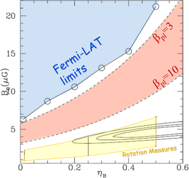
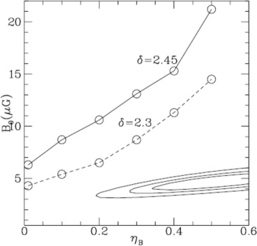
Figure 3: (left) The area constrained by Fermi-LAT limits in the $B_{0}-\eta_{B}$ diagram (blue area) assuming a pure hadronic models for the Coma radio halo and $\delta=2.45$. This region is compared with the 1, 2, 3$\sigma$ constraints from Faraday RM (solid lines from Bonafede et al., 2010) and with the region constrained from the same Faraday RM using only background radio galaxies (yellow region; see main text for details). The region spanned by $B_{0}$ and $\eta_{B}$ in the case of a $\beta_{\mathrm{pl}}=3$ to 10 at a distance of 2.5-3$r_{c}$ is also reported for comparison (orange region). (right) The same comparison between magnetic field lower limits and constraints from Faraday RM assuming $\delta=2.45$ and 2.3.

The discrepancy between minimum B-fields allowed for a pure secondary origin of the halo and that from RM is very large, with the magnetic field energy density in the cluster being $>$15-20 times larger than that constrained using RM. An obvious consequence is that the magnetic field in the ICM would be dynamically important in the case of a pure hadronic origin of the halo. This is particularly true in the external, $r\geq 2-2.5r_{c}$ (that is $r\geq 0.4-0.5R_{500}$), regions where most of the cluster thermal energy budget is contained and where most of the radio halo emission is generated (Fig. 2). In order to further explain this point, in Fig. 3 (left) we also report the region of parameters corresponding to a beta plasma (ratio of thermal and magnetic pressure, $\beta_{\mathrm{pl}}=8\pi P_{\mathrm{ICM}}/B^{2}$) between 3 and 10 at a reference distance 2.5-3 $r_{c}$ ($\simeq$730-875 kpc, i.e., $\simeq 0.5-0.6\times R_{500}$). Limits on $B_{0}$ ($\eta_{B}$) from our combined radio – Fermi-LAT analysis select $\beta_{\mathrm{pl}}<2-3$ at these distances independently of the value of $\eta_{B}$ and imply an important (even dominant) contribution to cluster dynamics from the magnetic field pressure. This is in clear tension with several independent theoretical arguments and observational constraints (e.g., Miniati & Beresnyak, 2015, and references therein).

In Fig.3 (right) we show the effect of different spectra of the CRp. Flatter spectra make constraints slightly less stringent. This is simply because GeV photons produced by the decay of neutral pions probe CRp with energies that are about 5-10 times smaller than those of the CRp which generate the secondary electrons emitting at 300 MHz. However, if the spectrum of CRp has a slope $\delta>2.35$, as constrained by radio observations, our conclusions remain essentially unaffected.

Our calculations assume a power-law spectrum of the primary CRp (subject to modifications induced by Coulomb and CRp–p losses). Propagation effects in the ICM might induce additional modifications in the spectrum of CRp that may change the radio to gamma-ray luminosity ratio, $L_{\mathrm{radio}}/L_{\gamma}$, with respect to our calculations. An unfavorable situation is when confinement of CRp in Mpc³ volumes is inefficient for CRp energies $\geq 10$ GeV. In this case the spectrum of CRp at lower energies may be flatter than that constrained from radio observations causing a reduction of the expected gamma-ray luminosity. However, even by assuming this unfavourable (and ad hoc) situation, we checked that the decrease of the gamma-ray luminosity with respect to our calculations can be estimated within a factor $\leq$1.5-2 considering injection spectra of CRp $\delta\geq 2$, thus it would not affect our main conclusions too much.

At this point it is also useful to derive the maximum energy of CRp that is allowed by the Fermi-LAT limits as a function of $\eta_{B}$. In Figure 4 we show three relevant examples that are obtained assuming $\eta_{B}=0$, 0.3 and 0.5 and the corresponding values of the minimum $B_{0}$ for which the gamma-ray flux equals Fermi-LAT limits (i.e., $B_{0}=6$, 13 and 21$\mu$G respectively; Fig. 3, left). We find that the ratio of the energy density of CRp and thermal ICM increases with distance, this is in line with independent other findings that attempt to match the observed radio profile of the Coma cluster with pure secondary models (e.g., Zandanel & Ando, 2014). In practice the decline with radius of the thermal targets for CRp-p collisions combined with the very broad radial profile of the synchrotron brightness requires a substantial amount of CRp in the external regions. The ratio $\epsilon_{\mathrm{CRp}}/\epsilon_{\mathrm{ICM}}$ increases by one order of magnitude from about 1% in the core to about 10% at 3 core radii, where most of the thermal energy budget is contained. Despite the spatial profile of the magnetic field in the three models is very different ($\eta_{B}$), we note that $\epsilon_{\mathrm{CRp}}/\epsilon_{\mathrm{ICM}}$ does not differ very much. This is not surprising, because the magnetic field in these models is strong, $B^{2}\gg B_{cmb}^{2}$ (Fig. 3), implying that a change of the magnetic field with distance does not lead to a strong variation of the ratio between gamma and radio luminosity (Eq. 17).

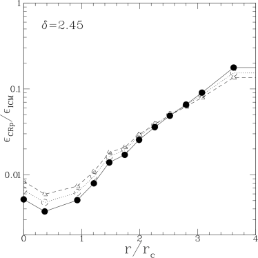
Figure 4: Upper limits to the ratio of the CRp to the thermal ICM energy densities as a function of radius. The three models assumes $\eta_{B}=0$ (dashed), 0.3 (dotted) and 0.5 (solid) and the corresponding values of the lower-limit to the central magnetic fields $B_{0}$ from Figure 3 (left).

5.2 The general case with reacceleration

In this section we consider the general case where turbulence is present in the ICM and reaccelerates CRp and secondary particles. We assume that the contribution of primary electrons is negligible (this is the case $f=1$ in Sect. 2) leading to optimistic expectations for the level of the gamma-ray emission. Turbulent acceleration time is assumed constant with radius, in practice this postulates that Mach numbers and turbulent injection scales (or their combination) are constant throughout the cluster (see Sect. 6).

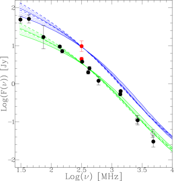
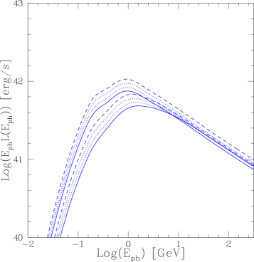
Figure 5: Spectra emitted by a bundle of representative models. (left) Radio spectrum from eigth reacceleration models obtained assuming four reacceleration times ranging from $\tau_{\mathrm{acc}}=230$ to 300 Myr and two reacceleration periods $\Delta T_{\mathrm{acc}}=$480 and $=$780 Myr. Calculations assume $z_{i}=0.2$. The synchrotron flux is calculated from models assuming two aperture radii $=$525 kpc (green, bottom) and 1.2 Mpc (blue, upper). Radio data (black points) are taken from Pizzo (2010); fluxes at high frequencies are corrected for the SZ decrement considering a aperture radius $=$0.55 Mpc following Brunetti et al. (2013) (empty points at 2.7 and 4.8 GHz are the original fluxes). The two radio fluxes obtained at 325 MHz using the new WSRT data (red points) are extracted within apertures $=$0.6 (bottom) and 1.2 Mpc (upper) respectively. (right) The gamma-ray spectrum obtained from the same models in the left-panel calculated using an aperture radius $=1.2$ Mpc.

First of all, we have to start from an initial spectrum of CRp in the cluster. As a simplification we assume that CRp in the ICM are continuously injected between $z_{i}$ and $z_{f}$ with an injection spectrum $Q_{p}(p,t)\propto p^{-2.45}$. We assume that reacceleration starts at $z_{f}$ and that in the redshift range $z_{i}$ – $z_{f}$ the CRp are subject to Coulomb losses and CRp-p collisions (Sect. 3). In this time period we assume an average density of the thermal plasma $n_{\mathrm{ICM}}\sim 10^{-3}$cm s^-1. In this Section we consider two reference cases $z_{i}=0.2$ and 0.5 and that reacceleration starts at a reference redshift $z_{f}=0.04$.

Starting from the spectrum at $z=z_{f}$, we calculate the time evolution of CRp at several distances from the cluster center due to losses and reaccelerations and the production (and evolution) of secondary electrons and positrons. In addition, turbulence reaccelerates also sub/trans-relativistic CRp to higher energies. Thus the choice of different values of $z_{i}$ is aimed at exploring the changes of the non-thermal emission that are induced by assuming two “extreme” situations with initial CRp spectra that significantly differ at lower energies. We note that the exact value of the final redshift $z_{f}$ ($\pm$ 0.5 Gyr) does not significantly affect our results.

At this point the free parameters of the models are:

• the magnetic field configuration, $B_{0}$ and $\eta_{B}$;

• the acceleration efficiency $\tau_{\mathrm{acc}}^{-1}$ (which depends on the combination of turbulent Mach number and injection scale); and

• the duration of the reacceleration phase, $\Delta T_{\mathrm{acc}}$.

We proceed by assuming a magnetic field model $(B_{0},\eta_{B})$ and explore a range of values for $\tau_{\mathrm{acc}}^{-1}$ and $\Delta T_{\mathrm{acc}}$. As explained in Sect. 3.3, in the case of collisionless TTD the CRp do not contribute very much to the turbulent damping and thus they can be treated as test particles in our calculations. As a consequence, for each model the normalization of the spectrum of CRp (essentially their number density) at each distance from the cluster center is adapted to match the observed brightness distribution at 350 MHz. This procedure provides a bundle of models, anchored to the radio properties of the halo at 350 MHz, for which we calculate the synchrotron spectrum integrated within different aperture radii and the corresponding gamma-ray emission (spatial distribution and spectrum).

Examples of the synchrotron spectra of the Coma halo calculated for a bundle of models and integrated in an aperture radius of 525 kpc (bottom) and 1.2 Mpc (top) are reported in Figure 5 (left). We note that 500-550 kpc is a typical value for the aperture radius that is used in the literature to derive the flux of the radio halo (see discussion in Brunetti et al., 2013). Models in Fig. 5 are calculated assuming a magnetic field $B_{0}=4.7\mu$G and $\eta_{B}=0.5$, i.e., the best fit parameters from Faraday RM, (Bonafede et al., 2010). Models have the same luminosity at 350 MHz as they are all constructed to match the brightness profile of the halo at this frequency. Considering the range of parameters explored in Fig. 5, the models fit the observed curvature of the spectrum well, only showing deviations towards lower frequencies $\nu\leq 100$ MHz. We also note that all these models explain the spectral curvature of the (high-frequency) data in Fig. 5, which have already been corrected for the SZ decrement following Brunetti et al. (2013). This curvature per se demonstrates the existence of a break in the spectrum of the emitting electrons and has been used to support reacceleration models for the origin of the halo (e.g, Schlickeiser et al., 1987; Brunetti et al., 2001).

In Figure 5 (right) we show the gamma ray spectrum generated by the same models of Fig. 5 (left) integrating within a radius of $=1.2$ Mpc. While synchrotron spectra are fairly similar across a large range of frequencies, the corresponding gamma ray spectra generated between 100 MeV and a few GeV vary greatly. This is because, contrary to the synchrotron spectrum that is sensitive to the non-linear combination of electron spectrum and magnetic fields, the gamma rays directly trace the spectral energy distribution of CRp. In addition, we note that the GeV photons generated by the decay of neutral pions and the synchrotron photons that are emitted by secondary electrons at $\geq$100 MHz do not probe the same energy-region of the spectrum of CRp. Furthermore, the spectrum of secondary electrons are modified in a different way with respect to that of CRp during reacceleration (e.g., Fig. 3 in Brunetti & Lazarian, 2011) and thus the ratio between GeV and radio emission is also sensitive to the adopted reacceleration parameters.

Figure 5 shows the potential of gamma-ray observations: they allow to disentangle among different models that otherwise could not be separable from their synchrotron spectrum alone. Thus, following Sect. 4.2 we derive Fermi-LAT limits for a large number of models calculated using a reference range of parameters and compare these limits to the gamma-ray emission expected from the corresponding models. The procedure allows us to accept/rule out models and consequently to constrain the parameter space $\tau_{\mathrm{acc}}^{-1}$, $(B_{0},\eta_{B})$, $\Delta T_{\mathrm{acc}}$. More specifically we span the following range of parameters:

• a narrow range of $\tau_{\mathrm{acc}}=200-300$ Myr (that is the typical range used to explain the spectrum of the Coma halo);

• a reasonable range of $\Delta T_{\mathrm{acc}}=350-1000$ Myr (see Sect. 6); and

• two families of magnetic field configurations with $\eta_{B}=0.5$ and 0.3 and $B_{0}$ as free parameters. Since models are normalized to the same radio flux at 350 MHz (anchored to the brightness profile), the corresponding gamma-ray emission is expected to increase for smaller magnetic fields.

In Figure 6 we show the ratio of the flux above 100 MeV that is expected from models and the LAT limits derived for the same models as a function of the magnetic field in the cluster. Here we assume $\tau_{\mathrm{acc}}=260$ Myr and $\Delta T_{\mathrm{acc}}=720$ Myr that are representative, mean values of the range of parameters. The gamma-ray flux increases for smaller values of $B_{0}$. All models with $F_{>100}/F_{lim}\geq 1$ are inconsistent with LAT observations. In this specific case, we derive corresponding limits on the magnetic fields $B_{0}\geq 4\mu$G and $\geq 2.5\mu$G in the case $\eta_{B}=0.5$ and $=0.3$, respectively. These limits are consistent with the magnetic field values derived from Faraday RM. For comparison the limits derived in the case of pure hadronic models are much larger, $B_{0}\geq 21\mu$G and $\geq 13\mu$G, respectively (Sect. 5.1). In Fig. 6 we also show the threshold that is expected from upper limits in the case of 10 and 15 yrs of Fermi-LAT observations (see the Section 6.1 for details on how the expected limits were computed). The limits derived using 10-15 yrs of Fermi-LAT are expected to start constraining magnetic field values that are larger than (i.e., potentially inconsistent with) those from RM.

Before making a more general point on the constraints on the magnetic field that are allowed by LAT limits in the case of reacceleration models, we first investigate the dependencies on $\tau_{\mathrm{acc}}$ and the acceleration period. In Figure 7 we show the ratio of the flux expected above 100 MeV and the Fermi-LAT limits as a function of reacceleration efficiency. Here we assume the central value $\Delta T_{\mathrm{acc}}=720$ Myr (solid lines) and the best fit values from Faraday RM ($B_{0}=4.7\mu$G and $\eta_{B}=0.5$). The gamma-ray luminosity (and also $F_{>100}/F_{lim}$) increases with $\tau_{\mathrm{acc}}$, i.e., models with less efficient reacceleration produce more gamma rays. This trend does not depend on the specific choice of magnetic field configuration and is due to a combination of effects. First, the spectrum of CRp is less modified (i.e., less stretched in energy) in models with slower reacceleration implying a larger number of CRp in the energy range 1-10 GeV. Second, the spectrum of radio-emitting electrons is less boosted in the case of models with slower reacceleration implying that a larger number density of CRp is required to generate the observed flux at 350 MHz. More specifically we find that the latter effect dominates within about 2-3 reacceleration times, after which the spectral shape of the emitting electrons reaches quasi-stationary conditions and the evolution of the gamma-ray to radio ratio evolves mainly due to the modifications of the spectrum of CRp. In Fig. 7 we also show the threshold resulting from upper limits assuming 10-15 yrs of Fermi-LAT data. Assuming magnetic fields from the best fit of Faraday RM analysis, the expected limits considering an observation of 10-15 years of continued LAT exposure are poised to put tension on the majority of the range of acceleration times and acceleration periods explored in this paper (see the Section 6.1 for details on how the expected limits were computed). Coming back to the minimum value of the magnetic fields that can be assumed without exceeding observed gamma-ray flux limits, we note that the increase of the gamma-ray luminosity with $\tau_{\mathrm{acc}}$ implies that the minimum value of the central magnetic field $B_{0}$ increases with $\tau_{\mathrm{acc}}$.

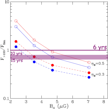
Figure 6: The ratio of the flux predicted by models for $\geq$100 MeV and the Fermi-LAT upper limits (obtained after 6 yrs of data in the same energy band) is shown as a function of the central magnetic field assumed in the models. Calculations assume $\tau_{\mathrm{acc}}=260$ Myr, $\Delta T_{\mathrm{acc}}=720$ Myr, $z_{i}=0.2$ (red) and $z_{i}=0.5$ (blue), and $\eta_{B}=0.3$ (dashed) and $\eta_{B}=0.5$ (solid). The horizontal pink region marks $F_{>100}/F_{lim}=1$ expected after 10 and 15 yrs of Fermi-LAT data.

The other relevant parameter is $\Delta T_{\mathrm{acc}}$. Once the synchrotron spectra are normalized to the observed luminosity at 350 MHz, shorther reacceleration periods produce more gamma rays simply because $L_{\mathrm{radio}}/L_{\gamma}$ increases with time. This is shown quantitatively in Fig.7 where we compare the case $\Delta T_{\mathrm{acc}}=$720 Myr with a shorther reacceleration period, $\Delta T_{\mathrm{acc}}=480$ Myr. The gamma-ray luminosity scales in the opposite way with $\tau_{\mathrm{acc}}$ and $\Delta T_{\mathrm{acc}}$. Faster reacceleration in shorther times may produce spectra that are comparable to the case of slower reacceleration in longer times inducing a corresponding degeneracy also in the expected gamma-ray flux. This is also clear from Fig.7: slower reacceleration with $\Delta T_{\mathrm{acc}}=$720 Myr generates about the same gamma-ray flux in the case of faster reacceleration with $\Delta T_{\mathrm{acc}}=$480 Myr.

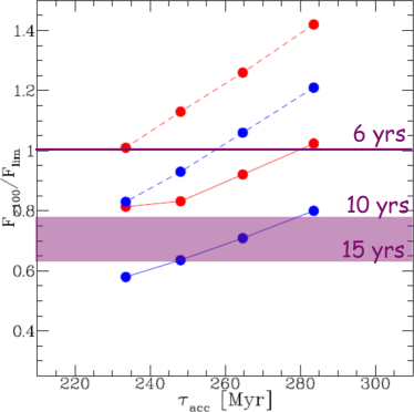
Figure 7: The ratio of the flux predicted by models for $\geq$100 MeV and the Fermi-LAT upper limits (obtained after 6 yrs of data in the same energy band) is shown as a function of the acceleration time. Calculations assume $\eta_{B}=0.5$, and $B_{0}=4.7\mu$G, $\Delta T_{\mathrm{acc}}=720$ Myr (solid) and 480 Myr (dashed), and $z_{i}=0.2$ (red) and $z_{i}=0.5$ (blue). The horizontal pink region marks $F_{>100}/F_{lim}=1$ expected after 10 and 15 yrs of Fermi-LAT data.

The combination of radio and gamma-ray limits allows a combined constraint on $\tau_{\mathrm{acc}}$ and $\Delta T_{\mathrm{acc}}$. In Figure 8 we show the minimum values of the reacceleration period that is constrained by gamma-ray limits as a function of reacceleration time. For consistency with previous Figures, this is also derived assuming the best fit values from Faraday RM. Note that smaller values of $\Delta T_{\mathrm{acc}}$ (for a given $\tau_{\mathrm{acc}}$) can be allowed assuming larger magnetic fields in the cluster.

Figs. 6-8 show that lower limits on the magnetic fields in the cluster increase with increasing $\tau_{\mathrm{acc}}$ and with decreasing $\Delta T_{\mathrm{acc}}$ and that these limits are not very far from the field values derived from Faraday RM. A relevant example is shown in Figure 9 where we report the minimum value of the magnetic field as a function of the acceleration time and for two values of the acceleration period. Calculations are obtained assuming $\eta_{B}=0.5$ and are compared with the value of $B_{0}$ that is derived from RM for the same $\eta_{B}$. Fig. 9 clearly shows that models with $\Delta T_{\mathrm{acc}}\leq 400-450$ Myr are in tension with current constraints from Faraday RM because a magnetic field that is too large is required in these models in order to avoid exceeding the gamma-ray limits. On the other hand, the minimum values of $B_{0}$ that are constrained for models with longer reacceleration periods become gradually consistent with Faraday RM. Interestingly, we conclude that the gamma-ray flux that is expected from reacceleration models assuming the magnetic field configuration that is derived from RM is similar (within less than a factor 2) to current Fermi-LAT limits, a fact that is particularly important for future observations as we outline in the Discussion section.

As a final point in Figure 10 we show the ratio $\epsilon_{\mathrm{CRp}}/\epsilon_{\mathrm{ICM}}$ as a function of radius for reacceleration models that assume $\tau_{\mathrm{acc}}=260$ Myr and $\Delta T_{\mathrm{acc}}=720$ Myr, and assuming different configurations of the magnetic field (see caption). We find that the ratio of the energy density of CRp and thermal ICM increases with distance. The increase of $\epsilon_{\mathrm{CRp}}$ with radius is faster than in the case of pure hadronic models (Fig. 4) and also the differences between the case $\eta_{B}=0.3$ and 0.5 are more pronounced. This can be explained by the magnetic fields in reacceleration models which are much smaller than those allowed in the case of pure secondaries implying that differences in the radial decline of $B$ with radius induce significant changes in the synchrotron emissivity. We note that the models in Figure 10, that assume $B_{0}=2.35~{}\mu$G and $\eta_{B}=0.3$ and $B_{0}=4.7~{}\mu$G and $\eta_{B}=0.5$, mark the situations where the resulting predicted gamma-ray fluxes would be in tension with the observed limits, implying that the corresponding values of $\epsilon_{\mathrm{CRp}}/\epsilon_{\mathrm{ICM}}$ are upper limits. In fact these limits constrain the ratio $\epsilon_{\mathrm{CRp}}/\epsilon_{\mathrm{ICM}}$ at distance $r\sim 3r_{c}$ to about 7-8$\%$ in both cases. The fact that the limit to the amount of CRp energy is slightly (factor 2) larger in the case of pure secondary models (Fig. 4) is due to the changes in the spectral shape of CRp (and gamma rays) derived from reacceleration (Fig. 5 right), and due to the differences between the spatial distribution of CRp in the two models.

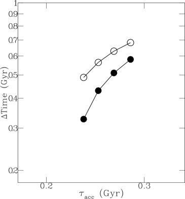
Figure 8: The lower limits to $\Delta T_{\mathrm{acc}}$ as a function of $\tau_{\mathrm{acc}}$ are obtained comparing the flux expected by models with the Fermi-LAT limits. Calculations are obtained for $\eta_{B}=0.5$ and $B_{0}=4.7\mu$G and assuming $z_{i}=0.2$ (upper) and $=$0.5 (lower).

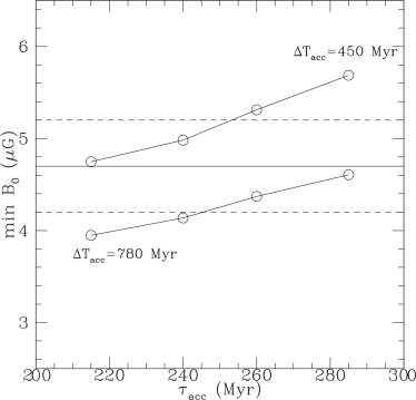
Figure 9: Lower limits to the central magnetic field, in the case $\eta_{B}=0.5$, as a function of reacceleration time. Calculations assume $z_{i}=0.2$, and $\Delta T_{\mathrm{acc}}=450$ Myr (upper) and $=$780 Myr (lower curve). Limits are compared to the range of values $1\sigma$ (dashed lines) constrained by Faraday RM (Bonafede et al., 2010).

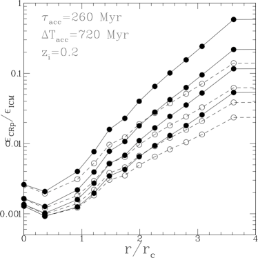
Figure 10: Upper limits to the ratio of the CRp to the thermal ICM energy densities as a function of radius. Models assume $\tau_{\mathrm{acc}}=260$ Myr, $\Delta T_{\mathrm{acc}}=720$ Myr and $z_{i}=0.2$. Results are shown for the cases $\eta_{B}=0.5$ (solid lines) and $=$0.3 (dashed), and considering four values of the central magnetic fied: $B_{0}=0.5\times$, $0.75\times$, $1.0\times$ and $1.5\times 4.7\mu$G (from bottom to upper lines).

6 Discussion

In this section we expand the discussion of our results including limitations of the current approach.

6.1 A detection in next years?

Our study demonstrates that turbulent reacceleration of secondary particles can explain the observed radio halo without exceeding the current gamma-ray limits. However, we have shown that assuming a magnetic field in the cluster that is compatible with Faraday RM, the level of the resulting gamma-ray flux is similar to what is currently constrained by observations of Fermi-LAT. This conclusion opens up the interesting perspective that the role of CRp for the observed cluster-scale radio emission may be efficiently tested with future observations.

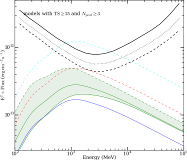
Figure 11: Predicted spectra (corrected for extension, see text) are compared with the sensitivity curves (concave black lines) of the Fermi-LAT after 6 (solid), 10 (dotted) and 15 yrs (dashed) of observations. Models assume $z_{i}=0.2$ and $\eta_{B}=0.5$. Two families of calculations are shown: (1) four models assuming $\tau_{\mathrm{acc}}=260$ Myr, $\Delta T_{\mathrm{acc}}=720$ Myr and the four central magnetic field values $B_{0}=(0.5,0.75,1.0,1.5)\times 4.7\mu$G (cyan dashed, red dashed, green solid (upper one) and blue solid, respectively); (2) two models assuming a central magnetic field $B_{0}=4.7\mu$G and the two combination of parameters $\tau_{\mathrm{acc}}=290$ Myr and $\Delta T_{\mathrm{acc}}=470$ Myr (red dashed), and $\tau_{\mathrm{acc}}=210$ Myr and $\Delta T_{\mathrm{acc}}=760$ Myr (green solid, lower one). The green region encompasses the range of spectra that are produced assuming a magnetic field configuration from the best fit of Faraday RM, $B_{0}=4.7\mu$G and $\eta_{B}=0.5$.

Turning the latter argument around, this also open to the possibility of a detection of the Coma cluster in the next years of observations, provided that CRp play an important role for the origin of the observed radio halo. To check this point we consider the sensitivity with 10 and 15 years of integrated sky exposure. In Fig. 11 we show the median sensitivity as provided by the so-called “Asimov” data set (Cowan et al., 2011) assuming that the background is determined entirely by both the Galactic diffuse emission model along with the isotropic extragalactic model, both provided by the LAT collaboration and made available through the Fermi Science Support Center (FSSC). For its calculation we assume that the test statistic $TS$, given by the likelihood ratio between the null-hypothesis (the gamma-ray emission observed in the cluster field consists of Galactic and isotropic extragalacticemission) $\mathcal{L}_{0}$ and the alternative hypothesis $\mathcal{L}_{1}$ (null-hypothesis in addition to the cluster emitting gamma rays according to the tested model) is larger than 25, which can be related to Gaussian significance $n$ as $n=\sqrt{TS}$, as well as requiring at least 3 photons to be attributed to the signal. This sensitivity calculation is implemented in FermiPy which is used with the corresponding set of IRFs and evaluated at the sky position of the Coma cluster. Note that the sensitivity curve is calculated assuming the emission to be point-like. In order to provide a reasonable comparison, we correct each of the model spectra for the extension by calculating a correction factor given as the ratio of the the uppr limit assuming the emission to be point-like and the flux upper limit under the model assumption.

In Fig. 11 we compare the sensitivity curves to the (corrected) expected gamma-ray spectra obtained assuming $\tau_{\mathrm{acc}}=260$ Myr, $\Delta T_{\mathrm{acc}}=720$ Myr, $\eta_{B}=0.5$ and $B_{0}=(0.5,0.75,1.0,1.5)\times 4.7\mu$G (from top to bottom); this is the same model configuration in Figure 6 (upper red solid line). High TS-values, $TS>25$, are predicted only for models that are already in tension with current upper limits (reported with dashed lines for sake of clarity), however there is a chance to obtain a signal in excess of $TS=9\simeq 3\sigma$ also for models that are still compatible with current limits. As a reference case, in Fig. 11 we show the spectral region (green) that is spanned by models with the magnetic field from the best fit from RM analysis ($B_{0}=4.7\mu$G and $\eta_{B}=0.5$) and assuming the full range of model parameters adopted in our paper.

6.2 Contribution from primary electrons in reacceleration models

In all the calculations carried out in this paper we have assumed $f=1$, i.e., the case of a negligible contribution to the radio emission from reaccelerated primary electrons. Thus our calculations are suitable to describe situations where the contribution of primary electrons is subdominant, similar to the case observed in our Galaxy. As discussed in Sect. 2, the gamma-ray flux essentially scales with $f^{-1}$ and consequently the case $f=1$ leads to the maximum gamma-ray emission that is predicted from reacceleration models for a given reacceleration efficiency and configuration of the magnetic field.

The ratio between primary and secondary particles in the ICM is unknown. Theoretical arguments suggest that CRp are the most important non-thermal component in galaxy clusters (Blasi et al., 2007; Brunetti & Jones, 2014, for review), implying that secondaries might indeed play a role. However this appears to be very sensitive to the acceleration efficiency at cluster shocks, which is poorly known (e.g., Kang & Ryu, 2011, 2013; Caprioli & Spitkovski, 2014). As a consequence it may very well be that $f\gg 1$ and that the gamma-ray flux from the Coma cluster is much smaller than that predicted by our calculations. In fact, originally the reacceleration models have been proposed assuming turbulent reacceleration of primary seed-electrons that may naturally accumulate at energies of about 100 MeV in the ICM as a result of the activity of shocks, AGN and galaxies (e.g., Brunetti et al., 2001; Petrosian, 2001). Most cosmological simulations point toward a dominant CRp contribution in clusters centre and an increasingly important role of primary electrons in clusters outskirts due to the complex network of shocks typically present there (e.g., Pfrommer et al., 2008; Skillman et al, 2008; Vazza et al, 2009; Pinzke & Pfrommer, 2010) leading to an increasing ratio $f$ with radius. This could possibly also alleviate the issue of the distribution of CRp needed to match giant radio halos, like Coma, that is required to significantly increase with radii (e.g., Brunetti et al., 2012; Zandanel et al., 2014, , this work). In this respect we also mention that several possible solutions to match the broad radial profiles of the Coma halo include CRp streaming, an enhanced efficiency for electrons acceleration at shocks, or an increasing turbulent-to-thermal energy ratio with radii (Pinzke et al., 2017).

The detection of gamma-ray emission from the Coma cluster in the future will constrain $f$ of the order of unity (assuming a magnetic field configuration in line with RM), however a non-detection at the sensitivity level that Fermi-LAT will reach in 10-15 years would not necessarily imply that reaccelerated secondary particles are completely subdominant.

6.3 Assumptions in acceleration models and parameter space

Our conclusions are based on the exploration of a limited range of model parameters and on a number of assumptions. While the former constitutes no significant limitation, evaluating in detail what changes are induced by relaxing some of our assumptions requires a follow-up study and is beyond the scope of this work. We comment on both points in the following.

The first parameter in our model is the acceleration time $\tau_{\mathrm{acc}}$ that we assume in the range 200-300 Myr. In the situation where reacceleration time is significantly shorter than the lifetime of the halo (or reacceleration period) the acceleration efficiency sets the maximum (i.e., steepening) synchrotron frequency of the spectral component that is powered by turbulent reacceleration. For constant reacceleration in the volume, the maximum frequency is typically generated in the regions of the cluster where $B\sim B_{\mathrm{IC}}/\sqrt{3}$. At the redshift of the Coma cluster (where $B_{\mathrm{IC}}/\sqrt{3}\simeq 2\mu$G) this steepening frequency is (from Eq. 14 in Brunetti & Lazarian, 2016) $\nu_{s}/{\rm GHz}\sim(\tau_{\mathrm{acc}}/400{\rm Myr})^{-2}$. This requires $\tau_{\mathrm{acc}}\sim 300$ Myr to explain the observed spectral steepening at $\sim 1-2$ GHz. Only if the magnetic field strength in the cluster core is sub-$\mu$G the required acceleration time should be $<200$ Myr. In this case, however, the gamma-ray luminosity would be strongly in excess of the Fermi-LAT limits, and such weak fields would also be much smaller than those derived from RM. We thus conclude that our calculations essentially span the range of values of $\tau_{\mathrm{acc}}$ that is relevant to explain the radio spectral properties of the halo.

The other parameter is the acceleration period, $\Delta T_{\mathrm{acc}}$, that we assume in the range 350-1000 Myrs. Specifically our conclusions depend on the ratio between the gamma-ray and radio luminosities which essentially depends on the reacceleration rate (and losses) that is experienced by secondary particles in the last $\Delta T_{\mathrm{acc}}$. $\Delta T_{\mathrm{acc}}$ is presumably smaller than the age of the radio halo which in fact can be longer than 1 Gyr (see, e.g., Miniati & Beresnyak, 2015; Cassano et al., 2016). Indeed it is very unlikely that particles in the ICM are continuously reaccelerated at a constant rate for much more than a turbulent cascading time, that is a few hundred Myr, and this motivates the range of $\Delta T_{\mathrm{acc}}$ that we assumed in our calculations. Even if turbulence in the ICM is long living, on longer times the dynamics of ICM would transport and mix CRp and their secondaries on large scales implying that CRs sample different physical conditions and different reacceleration efficiencies.

In our calculations we have assumed that the acceleration efficiency is constant in the cluster volume. In the case of TTD and under the assumption that turbulent interaction with both thermal ICM and CRs is fully collisionless (Sect. 3) the acceleration time is (Brunetti, 2016):

$$\tau_{\mathrm{acc}}={{p^{2}}\over{4D_{pp}}}\sim 125({{M_{o}}\over{1/2}})^{-4}\left({{L_{o}/300\,{\rm kpc}}\over{c_{s}/1500\,{\rm km\,s^{-1}}}}\right)\,\,({\rm Myr})$$ (18)

where we assumed a Kraichnan spectrum for MHD turbulence. Consequently a constant acceleration time implies (neglecting the dependence on temperature) that $L_{0}/M_{o}^{4}$ is constant. However numerical simulations suggest that turbulence in the ICM is stronger outside cluster cores and that the turbulent pressure is more relevant in the external regions (e.g., Vazza et al., 2017). If the turbulent Mach number increases radially, this would result in higher acceleration rates in the external regions (see also Pinzke et al., 2017). In this case matching the observed synchrotron profile would require an energy budget of the CRp in the external regions that is slightly smaller with the consequence that a lower gamma-ray luminosity is predicted.

From Eq. 18 it emerges that compressive turbulence in the Coma cluster should have a Mach number $\sim 0.4(L_{0}/300)^{1\over 4}$ to guarantee the acceleration rates $\tau_{\mathrm{acc}}\sim 200-300$ Myr that have been assumed in our calculations. This would result in about $15\%$ (or $5\%$) of pressure support from compressive motions generated on 300 kpc (or 30 kpc) scales. Direct measurements of turbulent velocities are currently available only for the cool-core of the Perseus cluster, where radial - line-of-sight - turbulent velocities $\sim 160$ km$/$s on $L_{0}\sim 30$ kpc scales have been derived from the analysis of the X-ray lines by the Hitomi collaboration (Hitomi Collaboration et al., 2016). This would imply a turbulent pressure support (limited to the eddies on $L_{0}\leq 30$ kpc scale) of about 4 % of the thermal pressure. Merging clusters - such as Coma - should be more turbulent (e.g., Paul et al, 2011; Vazza et al, 2011; Nagai et al, 2013; Miniati, 2014, 2015; Iapichino et al, 2017). For example, coming back to Coma, a recent analysis that combines numerical simulations and SZ fluctuations observed by Planck in the Coma cluster concluded for a dynamically important pressure support from turbulent fluctuations, presumably in the form of adiabatic modes on large scales (Khatri & Gaspari, 2016).

Finally we note that in calculations of reacceleration models we assumed an injection spectrum of CRp $\delta=2.45$, that is the reference spectrum that we have adopted in the case of pure hadronic models. On one hand this allows us to promptly establish the effect on the SED that is driven by adding turbulence in hadronic models, on the other hand this is a limitation of the current paper. Indeed the spectrum of secondary electrons in reacceleration models is not strightforwardly determined by the spectrum of CRp but rather by the combined effects of injection and spectral modifications that are induced by reacceleration and energy losses. Consequently a different injection spectrum of CRp can still fit the observed synchrotron spectrum of the Coma halo provided that the turbulent reacceleration rate is tuned accordingly. A full exploration of parameters in reacceleration models, including different CRp injection spectra, is beyond the focus of the paper and is a task for a forthcoming paper (Zimmer et al., in prep.). In principle steeper CRp spectra have a tendency to generate significantly more gamma rays in the Fermi-LAT energy range. However our calculations are also constrained by the observed spectrum of the radio halo in which case two combined effects compensate this tendency. First, steeper CRp spectra also generate more secondary electrons with $\sim$MeV–GeV kinetic energies that can be reaccelerated by turbulence leading to an increasing ratio between radio and gamma-ray luminosities which in turn implies a lower gamma-ray luminosity. Second, in the case of steeper CRp spectra slightly shorter $\tau_{acc}$ (or longer $\Delta T_{acc}$) are required to fit the radio spectrum of Coma and these configurations in reacceleration models have the tendency to produce less gamma-rays (Sect. 5.2). As a net result the gamma-ray luminosities in the Fermi-LAT band that are generated by reacceleration models using $\delta$ in the range 2.2–2.6 are expected to differ within less than a factor 2.

6.4 Beyond the case of collisionless TTD reacceleration

In our calculations we assumed a fully collisionless TTD interaction between compressive turbulence and both thermal ICM and CRs. This leads to a conservative estimate of the turbulent acceleration rate simply because in this way most of the turbulent energy is channelled into the thermal ICM (heating of the plasma). On the other hand this situation is very convenient because it allows us to treat CRs as passive tracers in the turbulent field as they do not contribute too much to turbulent damping (see Sect. 3). On the other hand it is also possible that only CRs interact in a collisionless way with turbulence and that the background ICM plasma behaves more collisional (see, e.g., Brunetti & Lazarian, 2011b). This is a more complex situation. It requires adequate calculations where CRs are fully coupled with the turbulent evolution and in general leads to situations where the turbulent reacceleration rate evolves with time. We note however that the non-linear coupling between CRs and turbulence does not change the functional form of the diffusion coefficient in the particles momentum space, $D_{pp}$ (Sect. 3), but it generally increases its normalization implying a faster reacceleration (Brunetti & Lazarian, 2011b). Thus the most important consequence would be that less turbulence is required to match a given reacceleration time $\tau_{\mathrm{acc}}$.

We also note that the scaling that is expected in TTD reacceleration, $D_{pp}\propto p^{2}$, at least for relativistic and ultrarelativistic particles, is fairly general for acceleration by large-scale turbulence. For example it is also common to betatron acceleration or magnetic pumping (e.g., Melrose, 1980; Le Roux et al., 2015), and to the situation where particles interact stochastically with compression and rarefaction in compressive turbulence (e.g., Ptuskin, 1988; Cho & Lazarian, 2006; Brunetti & Lazarian, 2007). Since $D_{pp}$ (in combination with losses) determines the spectrum of accelerated particles, this implies that the spectral shapes of CR and consequently the ratio of gamma rays to radio emission that are predicted for a given reacceleration rate, are not restricted to the particular use of the TTD mechanism.

Numerical simulations suggest that incompressible turbulence is important in the ICM (Miniati, 2014; Vazza et al., 2017). Turbulent reacceleration by large-scale incompressible turbulence in the ICM has been investigated in Brunetti & Lazarian (2016). In this case the reacceleration is not powered by compressions but it results from the interaction of particles with magnetic field lines subject to turbulent diffusion. In its most simple form, this mechanism leads to a functional form of the diffusion coefficient that is equivalent to TTD, $D_{pp}\propto p^{2}$, and - similarly to the case of collisional TTD and other mechanisms based on compressive turbulence - the use of this mechanism would simply lead to a different amount of turbulent energy that is required to obtain a given acceleration rate. In this case, however it is worth noting that the acceleration rate depends also on the value of the beta-plasma and a situation of constant reacceleration rate in the cluster volume may appear less natural than in the case of the TTD.

6.5 Limitations

An obvious limitation of this paper is that we carried out calculations assuming spherical symmetry. On one hand this allowed us a prompt comparison with the magnetic field values estimated from Faraday RM analysis and to use self consistently the values of the thermal parameters of the ICM that are derived from X-ray observations under the same assumption. On the other hand this simplification might have a potentially impact on some of our conclusions. The global ratio between radio and gamma-ray luminosities is the key parameter in our analysis. In the case of hadronic models it is given by Eq. 17 (for reacceleration it also depends on the shapes of the spectrum of secondaries and CRp which are modified by reacceleration and losses in a different way). In the case $\eta_{B}\sim 0$ the ratio between gamma rays and radio does not depend on the geometry of the system, on the other hand for steeper configurations of the magnetic field in the cluster the geometry may play a role. Although the appearence of the spatial distribution of the gas of the Coma cluster as projected on the plane of the sky is roughly symmetric (at least if we exclude the sub-group in the South-East periphery), it is possible that large deviations from the spherical symmetry occur in the direction of the line of sight. In the case of a spheroidal oblate (prolate), if we assume a configuration of the magnetic field which declines with distance, the cluster gamma-ray to radio flux ratio would be smaller (larger) than that estimated in the case of a spherical model. These effects may become important for large departures from spherical symmetry and in the cases of magnetic configurations with large values of $\eta_{B}$ and small values of the central magnetic fields. However, these magnetic configurations are clearly ruled out in the case of pure hadronic models, since they produce very large gamma-ray fluxes, and consequently these effects may have an impact only in the case of reacceleration models. In this respect, future constrained numerical simulations (see, e.g., Donnert et al., 2010) will help in evaluating in more detail the uncertainties of the predicted gamma-ray emission due to geometrical effects.

We also carried out calculations assuming that at each radius the magnetic field strength and the particle number densities are homogeneus. On the other hand spatial fluctuations of the magnetic field intensity may affect the ratio between synchrotron and gamma rays. In general, since the synchrotron emissivity scales non-linearly with magnetic field intensity, the presence of magnetic fluctuations tend to increase the ratio between radio and gamma rays. Assuming viable configurations for the spatial variations of the magnetic field, Brunetti et al. (2012) have shown that the radio-synchrotron to gamma rays ratio in the case of pure secondary models may increase up to a factor 2 with respect to homogeneus calculations, with the effect becoming progressively less important for larger magnetic fields (this is easy to understand from Eq. 17). Since in the case of pure hadronic models the new Fermi-LAT limits constrain very large values of the magnetic field in the cluster it is very unlikely that the presence of magnetic field variations affect our conclusions. On the other hand local variations of the magnetic field may affect the case of reacceleration models. Under some circumstances, this would make the predicted gamma-ray emission slightly smaller than that calculated assuming homogeneus conditions. However, a detailed evaluation of this effect requires the adoption of specific probability distribution functions of the magnetic fields values in the ICM combined with a quantitative analysis of the spatial diffusion of electrons across magnetic field fluctuations, which is beyond the aim of the present paper.

Another simplification in our calculations (and in the formalism in Sect. 3) is that spatial diffusion of CRs and propagation effects during the reacceleration phase are not taken into account. Calculations of turbulent reacceleration are carried out for $\Delta T_{\mathrm{acc}}$ which in turns translates into a resolution element where we have implicitly assumed that the thermal, turbulent and magnetic field parameters are constant. The size of this volume element is $L_{res}\sim 2\sqrt{D\Delta T_{\mathrm{acc}}}$, where $D$ is the spatial diffusion coefficient. An upper limit to $L_{res}$ can be estimated by adopting a very optimistic view where particles can travel undisturbed along field lines. In this case diffusion is constrained by magnetic mirroring and by the tangling scale of the magnetic field by turbulent motions and the pitch-angle averaged diffusion coefficient is $D\sim\langle D_{\|\|}\rangle\sim\phi l_{A}c$, where $\phi\sim 0.1-0.2$ and $l_{A}=M_{A}^{-3}L_{0}$ is the MHD scale (the scale where the eddy velocity equal the Alfvén speed). If we consider typical Alfvén Mach numbers and turbulent driving scales in the ICM, about $M_{A}\sim 5$ and $L_{0}\sim 100$ kpc, respectively, one finds $D\sim 10^{31}$cm²s^-1 and $L_{res}\leq 300\sqrt{\Delta T_{\mathrm{acc}}/Gyr}$ kpc. Since we know that on scales $L_{res}>200-300$ kpc in the ICM the physical parameters that are used in Eqs.1–3 change significantly, including the magnetic field strength, thermal density and turbulent properties (assuming a typical injection scale of about few $\times$100 kpc), we conclude that reacceleration periods $\sim 1\,\mathrm{Gyr}$ are the largest ones that can be assumed for homogeneus calculations.

7 Conclusions

CRp are expected to be the most important non-thermal components in galaxy clusters, still the energy budget that is associated with these particles is difficult to predict due to our poor knowledge of the micro-physics of the ICM, including the properties of particles transport and acceleration in this plasma. The combination of gamma rays and radio observations provides an efficient way to constrain the energy budget of CRp in galaxy clusters and their role for the origin of cluster-scale radio emission.

In this paper we have made an attempt to constrain the role of relativistic protons for the origin of the prototype radio halo in the Coma cluster by combining radio and gamma-ray data. More specifically we have assumed that secondary particles dominate the synchrotron emission of the halo, model the properties of the radio halo and explore the consequences for the gamma-ray emission of the cluster. The radio modeling has been calculated as a function of the magnetic field properties in the cluster and anchored to the brightness profile and flux of the radio halo at 350 MHz. In this way we derived the number density of CRp with radial distance and calculated the resulting gamma ray spectrum of the cluster. We then used publicly available likelihood curves obtained from LAT observations to determine corresponding 95% flux upper limits for our models and check whether they are consistent with one another.

In order to have a prompt comparison with Faraday RM, we adopt a general formulation for the magnetic field strength and scaling with radial distance in the cluster, $B(r)=B_{0}(n_{\mathrm{ICM}}(r)/n_{\mathrm{ICM}}(0))^{\eta_{B}}$, that is based on two parameters, $B_{0}$ and $\eta_{B}$. As a consequence our study provides combined constraints on $B_{0}$ and $\eta_{B}$.

7.1 Conclusions on pure hadronic models

The simplest case that we investigated is that where turbulence does not play a role. This is the case of pure hadronic models. In this simple scenario, for a given magnetic field configuration, the spectrum and spatial distribution of CRp are then entirely constrained by the observed spectrum and brightness distribution of the radio halo.

Assuming the best-fit scaling from Faraday RM, where the magnetic field energy density in the cluster scales with the thermal density of the ICM ($\eta_{B}=0.5$), we derive $B\geq 21\mu$G in the cluster core to be compared with $B\sim 4-5\mu$G as inferred from Faraday RM. The value of the minimum magnetic field decreases for sublinear scalings ($\eta_{B}<0.5$) but this also happens for the magnetic field values derived from RM. Specifically the ratio of the energy densities of the magnetic field constrained by our analysis and that measured from Faraday RM ranges from $>14$ in the case $\eta_{B}=0.2$ (i.e. the minimum $\eta_{B}$ allowed by RM) to $>20$ in the case $\eta_{B}=0.5$. Larger values of that ratio are derived for $\eta_{B}>0.5$. This improves very much the constraints derived by Brunetti et al. (2012) where the ratio of energy densities were $>3$ ($\eta_{B}=0.2$) and $>4$ ($\eta_{B}=0.5$).

The constraints derived for the magnetic field have a broader impact on the dynamical role of the magnetic field in the ICM. We have shown that, independently of $\eta_{B}$, the magnetic field pressure (volume averaged) at distance $R\geq 2.5\,r_{c}$, where most of the thermal and CRp energy budgets are contained, should be comparable to the thermal pressure ($\beta_{\mathrm{pl}}<2-3$). In other words assuming an hadronic origin of the radio halo has the consequence that a significant fraction of the energy of the Coma cluster must be in the form of the magnetic field. These findings confirm and significantly strengthen previous conclusions and readily disfavor the hypothesis of a pure hadronic origin of the radio halo.

7.2 The reacceleration case

Despite our results obtained for pure hadronic models, we pointed out that CRp can still play a role for the origin of the halo if these particles and their secondaries are reaccelerated by turbulence. In this case the tension with Fermi-LAT limits can be considerably alleviated because $L_{\mathrm{radio}}/L_{\gamma}$ can be much smaller than in the case of a pure hadronic scenario. In practice this results in the possibility that magnetic fields that are much weaker than those in the pure hadronic case are allowed by the gamma-ray limits.

The reacceleration scenario is however very complicated as it depends on several parameters and requires extensive calculations to explore a meaningful range of model parameters, which we have started to explore in this paper.

We assume that the turbulent reacceleration rate is constant in the cluster volume. Under the hypothesis that only CRp and their secondary particles are present in the ICM the model parameters are the acceleration rate $\tau_{\mathrm{acc}}^{-1}$, the duration of the reacceleration phase $\Delta T_{\mathrm{acc}}$, and the magnetic field model $(B_{0},\eta_{B})$. In this paper we have assumed a range of values: $\tau_{\mathrm{acc}}=200-300$ Myr, $\Delta T_{\mathrm{acc}}=350-1000$ Myr and studied two magnetic field models, with $\eta_{B}=0.5$ and 0.3, with $B_{0}$ as free parameter. Although we have explored a limited parameter range, in Sect. 6 we have shown that such a range is the relevant one to explain the radio halo. This is the first systematic study of the radio to gamma-ray spectrum from turbulent reacceleration of CRp and their secondaries assuming a range of model parameters, and in this respect it significantly extends previous studies (Brunetti & Lazarian, 2007; Brunetti et al., 2012; Pinzke et al., 2017).

For central magnetic fields larger than a few $\mu$G all model configurations provide a sufficiently good representation of the synchrotron spectrum of the Coma radio halo, including the observed spectral steepening at high frequencies. However they generate gamma-ray spectra that are significantly different.

We find that the expected gamma-ray luminosity increases with increasing $\tau_{\mathrm{acc}}$ and with decreasing $\Delta T_{\mathrm{acc}}$, that is essentially because in these models reacceleration boosts-up the spectrum of electrons at energies around GeV increasingly more than the spectrum of CRp in the case of faster reaccelerations and/or longer reacceleration periods. As a matter of facts our study demonstrates that the combination of radio and gamma-ray observations is a powerful tool to discriminate between different situations and to constrain acceleration parameters more broadly.

Similarly to the case of pure hadronic models the comparison between model expectations and Fermi-LAT limits allows to derive lower limits to the values of the magnetic field in the cluster. Assuming a reference case with $\tau_{\mathrm{acc}}=260$ Myr and $\Delta T_{\mathrm{acc}}=720$ Myr, we obtained $B_{0}>4\mu$G in the case $\eta_{B}=0.5$ and $B_{0}>2.5\mu$G for $\eta_{B}=0.3$. These limits are much weaker than those derived under the assumption of pure hadronic models and in fact are compatible with values from the analysis of Faraday RM. Higher (lower) values of the mimimum magnetic field are obtained for larger (smaller) $\tau_{\mathrm{acc}}$ and for smaller (larger) $\Delta T_{\mathrm{acc}}$. In general the magnetic field values constrained by our analysis are not in tension with values inferred from RM. However the model configurations combining lower reacceleration rates and shorter acceleration periods require large magnetic fields that can be in tension with Faraday RM. For example, in the reference case $\eta_{B}=0.5$, model configurations with $\Delta T_{\mathrm{acc}}\leq 400-450$ Myr require magnetic fields that are larger than those from Faraday RM across the entire range of values of reacceleration rates that is explored in our calculations. Flatter spatial distributions of the magnetic field, $\eta_{B}<0.5$, generate smaller gamma-ray fluxes allowing situations with smaller magnetic fields also in the configurations where reacceleration periods are short. However the tension with RM in the case of short reacceleration periods is not significantly reduced also for $\eta_{B}<0.5$ because in this case also the values of the magnetic fields that are constrained by RM are smaller.

Interestingly we have shown that a non detection of the Coma cluster using 10-15 yrs of Fermi-LAT data would imply a magnetic field in the cluster that is in clear tension with Faraday RM. This also open to the possibility of future detection of the Coma cluster in the gamma rays, provided that CRp play a role for the origin of the radio halo. We concluded that at least under a number of assumptions (namely quasi-homogeneus magnetic fields and quasi-spherical symmetry) there is a chance to obtain a signal in excess of 3$\sigma$ for models that assume magnetic field configurations compatible with Faraday RM.

7.3 Constraints on the energy content and spatial distribution of CRp

The Fermi-LAT limits constrain the maximum level of the energy budget that can be associated to CRp. The budget that is allowed increases for flatter spatial distributions of the CRp and this is because less gamma rays are generated due to the fact that the density of thermal targets in the cluster declines with distance. Several papers suggest that CRp distribute more broadly than the thermal ICM (e.g., Vazza et al, 2014; Wiener et al, 2013; Enßlin et al., 2011), still our poor knowledge of CRp dynamics in the ICM does not allow solid conclusions.

If radio halos have hadronic origin, radio observations set combined constraints on the spatial distrbution of CRp and magnetic field in the clusters. The broad brightness profile of the Coma radio halo implies that the underlying spatial distribution of the CRp is very broad as well. We find that the ratio of CRp and thermal energy densities should increase significantly with radius even in the case of a magnetic field profile that is much flatter than that of the thermal gas (Figs. 4 and 10) with the consequence that most of the energy of CRp should be stored in the external regions, $r\geq 2.5-3r_{c}$; a situation that is challenging to understand (e.g., Zandanel et al., 2014).

The combination of radio and gamma-ray data allows to put combined constraints on $B_{0}$ and $\eta_{B}$ and to break the degeneracy between the spatial distributions of magnetic field and CRp. Importantly, we have shown that the current Fermi-LAT observations limit the level of the energy budget of CRp to $\leq 10\%$ of the thermal ICM in a way that does not depend very much (within a factor 2) on the specific model of the halo (pure hadronic or reacceleration) and on the value of $\eta_{B}$. However, such a level of CRp energy content, which is increasing at larger radii, could undermine clusters’ hydrostatic mass estimates where non-thermal components, such as turbulence, CRs, and magnetic fields, are usually ignored (e.g., Ando & Nagai, 2008). In this sense, despite the great steps forward obtained thanks to gamma-ray observations, we are still far from sub-percent-level constrains or from a detailed knowledge of CRs in clusters.

Of course it is possible that the energy budget of CRp in the Coma cluster is significantly below this upper limit, simply because the limit is obtained under the hypothesis that secondary particles dominate the synchrotron emission up to large distances from the center. Therefore, it could be that the CRp follow a steeper distribution and that the external regions of the halo are powered by the reacceleration of primary electrons. In this case the energy budget of CRp as constrained by the Fermi-LAT limits would be much smaller.

Appendix A $D_{pp}$ Formula

In this Appendix we derive a general formula for the diffusion coefficient in the momentum space due to TTD with fast modes in the ICM that is valid also in the non-relativistic regime.

The resonant condition for TTD is:

$$\omega=k_{\|}v_{\|}$$ (19)

where $\omega=c_{s}k$ is the frequency of fast modes and $v_{\|}=\mu v$ and $k_{\|}=\eta k$ are the parallel (projected along the magnetic field) speed of the particles and the wave–number, respectively. This resonance changes only the component of the particle momentum parallel to the seed magnetic field and this would cause an increasing degree of anisotropy of the particle distribution leading to a less and less efficient process with time. However it is very likely that isotropization of particle momenta during acceleration is preserved by some mechanism (e.g., Schlickeiser & Miller, 1998; Brunetti & Lazarian, 2007, for discussions), and for this reason in our calculations we will assume a isotropic distribution of particles.

In order to derive the acceleration coefficient we follow Brunetti & Lazarian (2007) and use an approach based on the detailed balancing. The starting point is the collisionless damping rate of the waves due to TTD, that measures the rate of dissipation of turbulent energy into particles via TTD. The damping rate of fast modes due to TTD with $\alpha$-species particles in the ICM was derived by Brunetti & Lazarian (2007):

$$\Gamma_{\alpha}=-{{\pi^{2}}\over{8}}{{|B_{k}|^{2}}\over{B_{0}^{2}}}{{c_{s}k}\over{W}}{{\mu(1-\mu^{2})}\over{|\mu|}}{{{\cal H}(1-\big{|}{{c_{s}}\over{c\mu}}\big{|})}\over{\sqrt{1-({{c_{s}}\over{c\mu}})^{2}}}}{\cal I}_{\alpha}$$ (20)

where $\mu$ is the wave pitch-angle (i.e., $k_{\|}/k$) and

$${\cal I}_{\alpha}={1\over{m_{\alpha}}}\int_{0}^{\infty}dp_{\perp}{{p_{\perp}^{5}}\over{\sqrt{1+({{p_{\perp}}\over{m_{\alpha}c}})^{2}}}}\left({{\partial f_{\alpha}}\over{\partial p_{\|}}}\right)_{p_{\|,res}}\,.$$ (21)

The integral (Eq. 21) has to be evaluated at the resonant momentum (i.e., using Eq. 19), specifically under the condition that the parallel momentum is:

$$p_{\|,res}=m_{\alpha}c\left({{c_{s}}\over{c\mu}}\right)\left({{1+({{p_{\perp}}\over{m_{\alpha}c}})^{2}}\over{1-({{c_{s}}\over{c\mu}})^{2}}}\right)^{1\over 2}\,.$$ (22)

Under the assumption of isotropic distribution of particles, the next step is to re-write Eqs. 20–21 using particle momentum $p=\sqrt{p_{\|}^{2}+p_{\perp}^{2}}$. Eq. 22 gives:

$$dp_{\perp}={{1-({{c_{s}}\over{c\mu}})^{2}}\over{\sqrt{1-({{c_{s}}\over{c\mu}})^{2}/\beta^{2}}}}dp_{p_{\|,res}}$$ (23)

and the damping rate is:

$$\Gamma_{\alpha}(k,\mu)=\tilde{\Gamma}_{\alpha}\int_{p_{m}}dpp^{4}\big{[}1-({{c_{s}}\over{c\mu}})^{2}/\beta^{2}\big{]}^{2}\left({{\partial f}\over{\partial p}}\right){\cal H}(1-{{c_{s}}\over{c\mu\beta}})$$ (24)

where

$$\tilde{\Gamma}_{\alpha}={{\pi^{2}}\over{8}}k{{|B_{k}|^{2}}\over{B_{0}^{2}}}{{c_{s}^{2}}\over{W}}{{\mu(1-\mu^{2})}\over{|\mu|}}\,\,\,,$$ (25)

the Heaviside function in Eq. 24 accounts for the condition $p_{\|,res}<p$, and the minimum momentum in the integral in Eq. 24 is:

$$p_{m}=p_{\|}(p_{\perp}\rightarrow 0)={{m_{\alpha}c_{s}}\over{1-({{c_{s}}\over{c\mu}})^{2}}}{1\over{\mu}}\,.$$ (26)

The detailed balance approach accounts for the fact that the rate of energy that is extracted from the turbulence through collisionless damping with particles species $\alpha$, $\int d^{3}kW\Gamma$, is channelled into the same particles:

$$\int d^{3}pE_{\alpha}{{\partial f}\over{\partial t}}=\int d^{3}k\Gamma(k,\mu)W(k)\,.$$ (27)

Assuming isotropy, the time derivative of the particle phase-space distribution function is directly connected with the particle momentum diffusion coefficient via a Fokker-Planck equation:

$${{\partial f}\over{\partial t}}={{1}\over{p^{2}}}{{\partial}\over{\partial p}}\big{[}p^{2}D_{pp}{{\partial f}\over{\partial p}}\big{]}$$ (28)

where $D_{pp}$ is the momentum diffusion coefficient due to the same mechanism that drains energy from the turbulence into particles at the rate $\int d^{3}kW\Gamma$.

Combining Eqs.27–28 allows to connect directly the momentum diffusion coefficient with the damping coefficient of turbulence:

$$\int_{p_{m}}d^{3}p{{E_{\alpha}}\over{p^{2}}}{{\partial}\over{\partial p}}\big{[}p^{2}D_{pp}{{\partial f}\over{\partial p}}\big{]}=\int d^{3}k\Gamma(k,\mu)W(k)\,.$$ (29)

The left-hand side of Eq. 29 can be calculated via partial integration that gives:

$$\int d^{3}p{{E_{\alpha}}\over{p^{2}}}{{\partial}\over{\partial p}}\big{[}p^{2}D_{pp}{{\partial f}\over{\partial p}}\big{]}=-{{4\pi}\over{m_{\alpha}}}\int p^{3}D_{pp}\beta{{\partial f}\over{\partial p}}dp\,.$$ (30)

As a consequence the combination of Eqs.29–30 and 24–25 allows to derive the expression for the momentum diffusion coefficient:

$$D_{pp}\simeq{{\pi^{2}}\over{2c}}{{c_{s}^{2}}\over{B_{0}^{2}}}{{p^{2}}\over{\beta}}\int_{{c_{s}}\over{\beta c}}^{1}{\cal H}(1-{{c_{s}}\over{\beta c}}){{1-\mu^{2}}\over{\mu}}d\mu$$

$$\left[1-\big{(}{{c_{s}}\over{\mu\beta c}}\big{)}^{2}\right]^{2}\int dkkW_{B}$$ (31)

where in obtaning Eq. 31 we have introduced the isotropic spectrum (energy density per wavenumber) of magnetic field fluctuations associated to fast modes using:

$$W(k)={{W_{B}}\over{4\pi k^{2}}}\left({{16\pi W}\over{|B_{k}|^{2}}}\right)$$ (32)

where $16\pi W/|B_{k}|^{2}\sim{\cal O}(1)$ (Brunetti & Lazarian, 2007). Note that in the limit $p\gg mc$ Eq. 8 is Eq. (40) in Brunetti & Lazarian (2007).

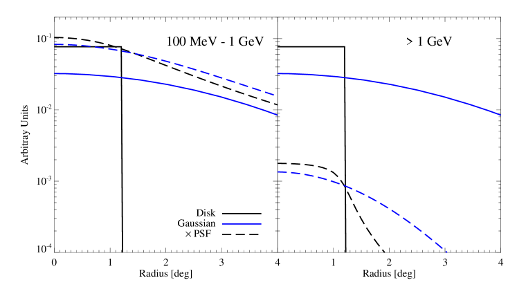
Figure 12: Radial surface brightness profile (arbitrary units) assuming a disk (black-solid line) and a Gaussian emission profile (blue-solid line), folded with the PSF for $P8R2\_SOURCE\_V6$ IRF (dashed lines) for low energies (100 MeV - 1 GeV) and at higher energies (> 1 GeV). Aside from a different normalization (which however is a free parameter in the likelihood procedure), at low energies, both models cannot be effectively distinguished from one another.

Appendix B Validation of Analysis

In this section we discuss the validity of our assumption that given the large PSF at low energies we can express any radially symmetric profile as an isotropic disk of unknown radius $R$.

Using the conversion of an incoming gamma-ray into an electron-positron pair, Fermi-LAT employs a silicon tracker interleaved with tungsten plates to promote pair conversion (Atwood et al., 2009). As a result, the angular resolution, or point-spread function (PSF) becomes a steeply varying function with energy (and incidence angle). As previoulsy shown in Lande et al. (2012), a model selection between a 2D Gaussian-like template for a source of size $\sigma$:

$$I_{\mathrm{Gaussian}}(x,y)=\frac{1}{2\pi\sigma^{2}}\times\exp\left(-(x^{2}+y^{2})/2\sigma^{2}\right)$$ (33)

and an isotropic disk-like template of similar size, cannot easily be made despite their analytical shapes being significantly different:

$$I_{\mathrm{Disk}}(x,y)=\begin{cases}\frac{1}{\pi\sigma^{2}}\quad&x^{2}+y^{2}\leq\sigma^{2}\\ 0\quad&x^{2}+y^{2}>\sigma^{2}.\end{cases}$$ (34)

While the underlying reconstruction software has received a major overhaul from Lande et al. (2012) to the data in Ackermann et al. (2016), we expect that for faint and largely extended gamma-ray emitters as it is expected from the diffuse gamma-ray emission from CR interactions in the ICM, the results of Lande et al. (2012) still apply.

Part of the output of gtsrcmaps is a 2D model map in which the input model is folded with the IRFs evaluated in the energy bin $E_{j}$. We sum up each of these maps above $E_{\mathrm{min}}$ weighted by a power-law spectrum with index -2.0 and extract the radial profile from the center of the map. In Fig. 12 we show the resultant radial profiles for an isotropic disk with radius as the virial radius of the Coma cluster $\theta_{\mathrm{Coma}}$ compared with a Gaussian with $\sigma=\theta_{\mathrm{Coma}}$ above 100 MeV (left) and 1 GeV (right). A visual comparison between this figure and Fig. 2 in Lande et al. (2012) supports our assumption, especially considering the quoted systematic uncertainties in Ackermann et al. (2016), which are dominated by the details of the Galactic foreground modeling.

Finally, we consider the effect of the existing grid of likelihood curves of varying disks by calculating modified flux upper limits for disk radii which do not match according to our comparison operators. Specifically, if for a given model $M_{i}$ we find a matching radius $r_{i}$, we calculated the resulting limits assuming that $r_{i\pm 1}$ are chosen instead. We find that the limits change less than $\pm 15\%$ with respect to the optimal value for $r_{i}$ (irrespective of the chosen comparison operator). Note that this value is well below the overall systematic uncertainties quoted in Ackermann et al. (2016), where bin-wise uncertainties are given as $<22\%$ for energy bins with $E>300\,\mathrm{MeV}$ and $<54\%$ towards the lower energies and integral limits are quoted with $<21\%$ for a hard spectral index ($\Gamma=1.6$) and $<42\%$ for a soft spectral index ($\Gamma=2.6$), respectively.

References

- Ackermann et al. (2010) Ackermann M., et al., 2010, ApJ, 717, L71
- Ackermann et al. (2014) Ackermann M., et al., 2014, ApJ, 787, 18
- Ackermann et al. (2016) Ackermann M., et al., 2016, ApJ, 819, 149
- Ade et al. (2013) Ade P. A. R., et al., 2013, A&A, 554, A140
- Aharonian et al. (2009a) Aharonian, F., et al. 2009, A&A, 502, 437
- Aharonian et al. (2009b) Aharonian, F., et al. 2009, A&A, 495, 27
- Ahnen et al. (2016) Ahnen M. L., et al., 2016, A&A, 589, A33
- Aleksić et al. (2010) Aleksić, J., et al. 2010, ApJ, 710, 634
- Aleksić et al. (2012) Aleksić, J., et al. 2012, A&A, 541, A99
- Ando & Nagai (2008) Ando, S., & Nagai, D. 2008, MNRAS, 385, 2243
- Arlen et al. (2012) Arlen T., et al., 2012, ApJ, 757, 123
- Atwood et al. (2009) Atwood W. B., et al., 2009, ApJ, 697, 1071
- Beresnyak et al. (2013) Beresnyak A., Xu H., Li H., Schlickeiser R., 2013, ApJ, 771, 131
- Berezinsky et al. (1997) Berezinsky V. S., Blasi P., Ptuskin V. S., 1997, ApJ, 487, 529
- Blasi & Colafrancesco (1999) Blasi P., Colafrancesco S., 1999, Astroparticle Physics, 12, 169
- Blasi et al. (2007) Blasi P., Gabici S., Brunetti G., 2007, International Journal of Modern Physics A, 22, 681
- Blattnig et al. (2000) Blattnig S. R., Swaminathan S. R., Kruger A. T., Ngom M., Norbury J. W., 2000, Phys. Rev. D, 62, 094030
- Bonafede et al. (2010) Bonafede A., Feretti L., Murgia M., Govoni F., Giovannini G., Dallacasa D., Dolag K., Taylor G. B., 2010, A&A, 513, A30
- Bonafede et al. (2013) Bonafede A., Vazza F., Brüggen M., Murgia M., Govoni F., Feretti L., Giovannini G., Ogrean G., 2013, MNRAS, 433, 3208
- Briel et al. (1992) Briel U. G., Henry J. P., Boehringer H., 1992, A&A, 259, L31
- Branchini et al. (2017) Branchini, E., Camera, S., Cuoco, A., et al. 2017, ApJS, 228, 8
- Brown & Rudnick (2011) Brown S., Rudnick L., 2011, MNRAS, 412, 2
- Brown et al (2011) Brown S., Emerick A., Rudnick L., & Brunetti G. 2011, ApJ740, L28
- Brunetti (2016) Brunetti G., 2016, Plasma Physics and Controlled Fusion, 58, 014011
- Brunetti & Blasi (2005) Brunetti G., Blasi P., 2005, MNRAS, 363, 1173
- Brunetti & Jones (2014) Brunetti G., Jones T. W., 2014, International Journal of Modern Physics D, 23, 30007
- Brunetti & Lazarian (2007) Brunetti G., Lazarian A., 2007, MNRAS, 378, 245
- Brunetti & Lazarian (2011) Brunetti G., Lazarian A., 2011, MNRAS, 410, 127
- Brunetti & Lazarian (2011b) Brunetti G., Lazarian A., 2011b, MNRAS, 412, 817
- Brunetti & Lazarian (2016) Brunetti G., Lazarian A., 2016, MNRAS, 458, 2584
- Brunetti et al. (2001) Brunetti G., Setti G., Feretti L., Giovannini G., 2001, MNRAS, 320, 365
- Brunetti et al. (2004) Brunetti G., Blasi P., Cassano R., Gabici S., 2004, MNRAS, 350, 1174
- Brunetti et al. (2009) Brunetti G., Cassano R., Dolag K., Setti G., 2009, A&A, 507, 661
- Brunetti et al. (2012) Brunetti G., Blasi P., Reimer O., Rudnick L., Bonafede A., Brown S., 2012, MNRAS, 426, 956
- Brunetti et al. (2013) Brunetti G., Rudnick L., Cassano R., Mazzotta P., Donnert J., Dolag K., 2013, A&A, 558, A52
- Caprioli & Spitkovski (2014) Caprioli D., & Spitkovsky A. 2014, ApJ, 783, 91
- Carilli & Taylor (2002) Carilli C. L., Taylor G. B., 2002, ARA&A, 40, 319
- Cassano & Brunetti (2005) Cassano R., Brunetti G., 2005, MNRAS, 357, 1313
- Cassano et al (2012) Cassano R., Brunetti G., Norris R. P., et al. 2012, A&A, 548, A100
- Cassano et al. (2016) Cassano R., Brunetti G., Giocoli C., Ettori S., 2016, A&A, 593, 81
- Cho & Lazarian (2006) Cho J., Lazarian A., 2006, ApJ, 638, 811
- Cowan et al. (2011) Cowan G., Cranmer K., Gross E., Vitells O., 2011, European Physical Journal C, 71, 1554
- Deiss et al (1997) Deiss B.M., Reich W., Lesh H., Wielebinski R., 1997, A&A, 321, 55
- Dennison (1980) Dennison B., 1980, ApJ, 239, L93
- Dermer (1986) Dermer C. D., 1986, A&A, 157, 223
- Dolag & Ensslin (2000) Dolag K., Ensslin T.A, 2000 A&A, 326, 151
- Donnert et al. (2010) Donnert J., Dolag K., Brunetti G., Cassano R., Bonafede A., 2010, MNRAS, 401, 47
- Donnert et al. (2013) Donnert J., Dolag K., Brunetti G., Cassano R., 2013, MNRAS, 429, 3564
- Eckert et al. (2017) Eckert, D., Gaspari, M., Vazza, F., et al. 2017, arXiv:1705.02341
- Eilek (1979) Eilek J. A., 1979, ApJ, 230, 373
- Enßlin et al. (2011) Enßlin, T., Pfrommer, C., Miniati, F., & Subramanian, K. 2011, A&A, 527, A99
- Feretti et al. (2012) Feretti L., Giovannini G., Govoni F., Murgia M., 2012, A&ARv, 20, 54
- Fisk (1976) Fisk L. A., 1976, J. Geophys. Res., 81, 4633
- Fujita et al. (2003) Fujita Y., Takizawa M., Sarazin C. L., 2003, ApJ, 584, 190
- Fujita et al. (2015) Fujita Y., Takizawa M., Yamazaki R., Akamatsu H., Ohno H., 2015, ApJ, 815, 116
- Giovannini et al. (1993) Giovannini G., Feretti L., Venturi T., Kim K.-T., Kronberg P. P., 1993, ApJ, 406, 399
- Govoni et al. (2001) Govoni F., Ensslin T.A., Feretti L., Giovannini G., 2001, A&A, 369 441
- Huber et al (2013) Huber B., Tchernin C., Eckert D., et al. 2013, A&A, 560, A64
- Jeltema & Profumo (2011) Jeltema T. E., Profumo S., 2011, ApJ, 728, 53
- Kamae et al. (2006) Kamae T., Karlsson N., Mizuno T., Abe T., Koi T., 2006, ApJ, 647, 692
- Kamae et al. (2007) Kamae T., Karlsson N., Mizuno T., Abe T., Koi T., 2007, ApJ, 662, 779
- Kang & Ryu (2011) Kang H., Ryu D. 2011, ApJ, 734, 18
- Kang & Ryu (2013) Kang H., Ryu D. 2013, ApJ, 764, 95
- Kelner et al. (2006) Kelner S. R., Aharonian F. A., Bugayov V. V., 2006, Phys. Rev. D, 74, 034018
- Keshet & Loeb (2010) Keshet U., Loeb A., 2010, ApJ, 722, 737
- Khatri & Gaspari (2016) Khatri R., Gaspari M., 2016, MNRAS, 463, 655
- Kunz, et al. (2014) Kunz M. W., Schekochihin A. A., Stone J. M., 2014, Phys. Rev. Lett., 112, 205003
- Hitomi Collaboration et al. (2016) Hitomi Collaboration, Aharonian F., Akamatsu H., et al., 2016, Nature, 535, 117
- Iapichino et al (2017) Iapichino L., Federrath C., & Klessen R. S. 2017, arXiv:1704.02922
- Lande et al. (2012) Lande J., et al., 2012, ApJ, 756, 5
- Le Roux et al. (2015) le Roux J. A., Zank G. P., Webb G. M., Khabarova O. 2015, ApJ, 801, 112
- Melrose (1980) Melrose D. B. 1980, New York: Gordon and Breach, 1980
- Miller et al. (1996) Miller J. A., Larosa T. N., Moore R. L., 1996, ApJ, 461, 445
- Miniati (2014) Miniati F., 2014, ApJ, 782, 21
- Miniati (2015) Miniati F., 2015, ApJ, 800, 60
- Miniati & Beresnyak (2015) Miniati F., Beresnyak A., 2015, Nature, 523, 59
- Moskalenko & Strong (1998) Moskalenko I. V., Strong A. W., 1998, ApJ, 493, 694
- Nagai et al (2013) Nagai D., Lau E. T., Avestruz C., Nelson K., Rudd D. H. 2013, ApJ, 777, 137
- Paul et al (2011) Paul S., Iapichino L., Miniati F., Bagchi J., Mannheim K. 2011, ApJ, 726, 17
- Petrosian (2001) Petrosian V., 2001, ApJ, 557, 560
- Petrosian & East (2008) Petrosian V., East W. E., 2008, ApJ, 682, 175
- Petrosian & Kang (2015) Petrosian V., Kang B., 2015, ApJ, 813, 5
- Pfrommer & Enßlin (2004) Pfrommer C., Enßlin T. A., 2004, A&A, 413, 17
- Pfrommer et al. (2008) Pfrommer, C., Enßlin, T. A., & Springel, V. 2008, MNRAS, 385, 1211
- Pinzke & Pfrommer (2010) Pinzke, A., & Pfrommer, C. 2010, MNRAS, 409, 449
- Pinzke et al. (2013) Pinzke, A., Oh, S. P., & Pfrommer, C. 2013, MNRAS, 435, 1061
- Pinzke et al. (2017) Pinzke A., Oh S. P., Pfrommer C., 2017, MNRAS, 465, 4800
- Pizzo (2010) Pizzo R. F., 2010, PhD thesis, University of Groningen
- Prokhorov & Churazov (2014) Prokhorov D. A., & Churazov E. M. 2014, A&A, 567, A93
- Ptuskin (1988) Ptuskin V. S., 1988, Soviet Astronomy Letters, 14, 255
- Rudnick & Blundell (2003) Rudnick L., Blundell K. M.m 2003, ApJ, 588 143
- Santos-Lima, et al. (2014) Santos-Lima R., de Gouveia Dal Pino E. M., Kowal G., et al., 2014, ApJ, 781, 84
- Santos-Lima, et al. (2017) Santos-Lima R., de Gouveia Dal Pino E. M., Falceta-Goncalves D. A., et al., 2017, MNRAS, 465, 4866
- Schekochihin & Cowley (2006) Schekochihin A. A., Cowley S. C., 2006, Physics of Plasmas, 13, 056501
- Schlickeiser et al. (1987) Schlickeiser R., Sievers A., Thiemann H., 1987, A&A, 182, 21
- Schlickeiser & Miller (1998) Schlickeiser R., Miller J. A., 1998, ApJ, 492, 352
- Skillman et al (2008) Skillman S. W., O’Shea B. W., Hallman E. J., Burns J. O., & Norman M. L. 2008, ApJ, 689, 1063
- Snowden et al. (2008) Snowden S. L., Mushotzky R. F., Kuntz K. D., Davis D. S., 2008, A&A, 478, 615
- Thierbach et al. (2003) Thierbach M., Klein U., Wielebinski R., 2003, A&A, 397, 53
- Vazza et al (2009) Vazza F., Brunetti G., & Gheller C. 2009, MNRAS, 395, 1333
- Vazza et al (2011) Vazza F., Brunetti G., Gheller C., Brunino R., & Brüggen M. 2011, A&A, 529, A17
- Vazza et al (2014) Vazza F., Gheller C., & Brüggen M. 2014, MNRAS, 439, 2662
- Vazza et al. (2017) Vazza F., Jones T. W., Brüggen M., Brunetti G., Gheller C., Porter D., Ryu D., 2017, MNRAS, 464, 210
- Voit (2005) Voit G. M., 2005, Reviews of Modern Physics, 77, 207
- Völk et al. (1996) Völk H. J., Aharonian F. A., Breitschwerdt D., 1996, Space Sci. Rev., 75, 279
- Wiener et al (2013) Wiener J., Oh S. P., & Guo F. 2013, MNRAS, 434, 2209
- Wik et al. (2009) Wik D. R., Sarazin C. L., Finoguenov A., Matsushita K., Nakazawa K., Clarke T. E., 2009, ApJ, 696, 1700
- Selig et al. (2015) Selig, M., Vacca, V., Oppermann, N., & Enßlin, T. A. 2015, A&A, 581, A126
- Wilson (1970) Wilson T. L., 1970, A&A, 4, 487
- Zandanel & Ando (2014) Zandanel F., Ando S., 2014, MNRAS, 440, 663
- Zandanel et al. (2014) Zandanel F., Pfrommer C., Prada F., 2014, MNRAS, 438, 124
- Zandanel et al. (2015) Zandanel, F., Tamborra, I., Gabici, S., & Ando, S. 2015, A&A, 578, A32