Computational Krylov-based methods for large-scale differential Sylvester matrix problems

Abstract

In the present paper, we propose Krylov-based methods for solving large-scale differential Sylvester matrix equations having a low rank constant term. We present two new approaches for solving such differential matrix equations. The first approach is based on the integral expression of the exact solution and a Krylov method for the computation of the exponential of a matrix times a block of vectors. In the second approach, we first project the initial problem onto a block (or extended block) Krylov subspace and get a low-dimensional differential Sylvester matrix equation. The latter problem is then solved by some integration numerical methods such as BDF or Rosenbrock method and the obtained solution is used to build the low rank approximate solution of the original problem. We give some new theoretical results such as a simple expression of the residual norm and upper bounds for the norm of the error. Some numerical experiments are given in order to compare the two approaches.

1 Introduction

In the present paper, we consider the differential Sylvester matrix equation (DSE in short) of the form

$$\left\{\begin{array}[]{l}\dot{X}(t)=A(t)\,X(t)+X(t)\,B(t)+E(t)F(t)^{T};\;(DSE)\\ \;X(t_{0})=X_{0},\;\;t\in[t_{0},\,T_{f}],\end{array}\right.$$ (1)

where $A(t)\in\mathbb{R}^{n\times n}$, $B(t)\in\mathbb{R}^{p\times p}$ and $E(t)\in\mathbb{R}^{n\times s}$ and $F(t)\in\mathbb{R}^{p\times s}$ are full rank matrices, with $s\ll n,\,p$. The initial condition is given in a factored form as $X_{0}=Z_{0}\widetilde{Z}_{0}^{T}$ and the matrices $A$ and $B$ are assumed to be large and sparse.
Differential Sylvester equations play a fundamental role in many areas such as control, filter design theory, model reduction problems, differential equations and robust control problems [1, 4]. For such differential matrix equations, only a few attempts have been made for large problems.

Let us first recall the following theoretical result which gives an expression of the exact solution of (1).

Theorem 1.

[1] The unique solution of the general differential Sylvester equation

$${\dot{X}}(t)=A(t)\,X(t)+X(t)\,B(t)+M(t);\;\;X(t_{0})=X_{0}$$ (2)

is defined by

$$X(t)=\Phi_{A}(t,0)X_{0}{\Phi_{B^{T}}^{T}(t,t_{0})}+\int_{t_{0}}^{t}\Phi_{A}(t,\tau)M(\tau){\Phi_{B^{T}}^{T}(t,\tau)}d\tau.$$ (3)

where the transition matrix $\Phi_{A}(t,t_{0})$ is the unique solution to the problem

$${\dot{\Phi}}_{A}(t,t_{0})=A(t)\Phi_{A}(t,t_{0}),\;\;\Phi_{A}(t_{0},t_{0})=I.$$

Futhermore, if $A$ is assumed to be a constant matrix, then we have

$$X(t)=e^{(t-t_{0})A}X_{0}e^{(t-t_{0})B}+\int_{t_{0}}^{t}e^{(t-\tau)A}M(\tau)e^{(t-\tau)B}d\tau.$$ (4)

We notice that the problem (1) is equivalent to the linear ordinary differential equation

$$\left\{\begin{array}[]{c c l}\dot{x}(t)&=&\mathcal{A}(t)x(t)+b(t)\\ x_{0}&=&vec(X_{0})\end{array}\right.$$ (5)

where $\mathcal{A}=I\otimes A(t)+B^{T}(t)\otimes I$, $x(t)=vec(X(t)$ and $b(t)=vec(E(t)F(t)^{T})$, where $vec(Z)$ is the long vector obtained by stacking the columns of the matrix $Z$, forming a sole column. For moderate size problems, it is then possible to directly apply an integration method to solve (5). However, this approach is not suitable for large problems. From now on, we assume that the matrices $A$ and $B$ are time independent.

In the present paper, we will consider projection methods onto extended block Krylov (or block Krylov) subspaces associated to the pairs $(A,E)$ and $(B^{T},F)$ defined as follows

$$\mathbb{K}_{m}(A,E)={\rm range}(E,AE,\ldots,A^{m-1}E)$$

for block Krylov subspaces, or

$${\cal K}_{m}(A,E)={\rm range}(A^{-m}E,\ldots,A^{-1}E,E,AE,\ldots,A^{m-1}E)$$

for extended block Krylov subspaces when the matrix $A$ is nonsingular. Notice that the extended block Krylov subspace ${\cal K}_{m}(A,E)$ is a sum of two block Krylov subspaces associated to the pairs $(A,E)$ and $(A^{-1},A^{-1}E)$:

$${\cal K}_{m}(A,E)=\mathbb{K}_{m}(A,E)\,+\,\mathbb{K}_{m}(A^{-1},A^{-1}E).$$

To compute an orthonormal basis $\{V_{1},\ldots,V_{m}\}$, where $V_{i}$ is of dimension $n\times d$ where $d=s$ for the block Krylov and $d=2s$ in the extended block Krylov case, two algorithms have been defined: the first one is the well known block Arnoldi algorithm and the second one is the extended block Arnoldi algorithm [5, 17]; see Appendix A for the description of both algorithms.
These algorithms generate the blocks $V_{1},V_{2},\ldots,V_{m}$, $V_{i}\in\mathbb{R}^{n\times d}$ such that their columns form an orthonormal basis of the block Krylov subspace $\mathbb{K}_{m}(A,E)$ (with $d=s$) or the extended block Arnoldi ${\cal K}_{m}(A,E)$ (with $d=2s$).
Both algorithms compute also $d\times d$ block upper Hessenberg matrices ${\mathcal{T}}_{m,A}={\mathcal{V}}_{m}^{T}\,A\,{\mathcal{V}}_{m}$. The following algebraic relations are satisfied

$$A\,{\cal V}_{m} = {\cal V}_{m+1}\,{\widehat{\cal T}}_{m,A},$$ (6)

$$= {\cal V}_{m}\,{\cal T}_{m,A}+V_{m+1}\,T_{m+1,m}\,\widetilde{E}_{m}^{T},$$ (7)

where ${{\widehat{\cal T}}_{m,A}}={\cal V}_{m+1}^{T}\,A\,{\cal V}_{m};$ $T_{i,j}$ is the $(i,j)$ block of ${\widehat{\cal T}_{m,A}}$ of size $d\times d$, and $\widetilde{E}_{m}=[O_{d\times(m-1)d},I_{d}]^{T}$ is the matrix formed with the last $d$ columns of the $md\times md$ identity matrix $I_{md}$ where $d=s$ for the block Arnoldi and $d=2s$ for the extended block Arnoldi.
When the matrix $A$ is nonsingular and when the computation of the products $W=A^{-1}V$ is not difficult (which is the case for sparse and structured matrices), the use of the extended block Arnoldi is to be preferred.

The paper is organized as follows: In Section 2, we present a first approach based on the approximation of the exponential of a matrix times a block using a Krylov projection method. We give some theoretical results such as a simple expression of the norm of the residual and upper bounds for the norm of the error and perturbation results. In Section 3, the initial differential Sylvester matrix equation is projected onto a block (or extended block) Krylov subspace. The obtained low dimensional differential Sylvester equation is solved by using the well known Backward Differentiation Formula (BDF) and Rosenbrock methods. The last section is devoted to some numerical experiments.
Throught the paper, $\|.\|$ and $\|\,.\,\|_{F}$ will denote the 2-norm and the Frobenius norm, respectively.

2 Solutions via of the matrix exponential approximation

In this section, we give a new approach for computing approximate solutions to large differential Sylvester equations (1).
We recall that the exact solution to (1) can be expressed as follows

$$X(t)=e^{(t-t_{0})A}X_{0}e^{(t-t_{0})B}+\int_{t_{0}}^{t}e^{(t-\tau)A}\,EF^{T}e^{(t-\tau)B}\,d\tau.$$ (8)

For our first approach, we use this expression of $X(t)$ to obtain low rank approximate solutions. We first approximate the factors $e^{(t-\tau)A}E$ and $e^{(t-\tau)B^{T}}F$ and then, use a quadrature method to compute the desired approximate solution. As the matrices $e^{(t-\tau)A}$ and $e^{(t-\tau)B^{T}}$ are large and could be dense even though $A$ and $B$ are sparse, computing the exponential is not recommended. However, in our problem, the computation of $e^{(t-\tau)A}$ and $e^{(t-\tau)B^{T}}$ are not needed explicitly as we will rather consider the products $e^{(t-\tau)A}\,E$ and $e^{(t-\tau)B^{T}}F$ for which approximations via projection methods onto block or extended block Krylov subspaces are well suited.
In what follows, we consider projections onto extended block Krylov (or just block Krylov) subspaces. Let $\mathcal{V}_{m}=[V_{1},\ldots,V_{m}]$ and $\mathcal{W}_{m}=[W_{1},\ldots,W_{m}]$ be the orthogonal matrices whose columns form an orthonormal basis of the subspace ${\cal K}_{m}(A,E)$ and ${\cal K}_{m}(B^{T},F)$, respectively. Following [15, 16, 19], an approximation to $Z_{A}=e^{(t-\tau)A}\,E$ can be obtained as

$$Z_{m,A}(\tau)=\mathcal{V}_{m}e^{(t-\tau)\mathcal{T}_{m,A}}\,\mathcal{V}_{m}^{T}E$$ (9)

where $\mathcal{T}_{m,A}=\mathcal{V}^{T}_{m}A\mathcal{V}_{m}$. In the same way, an approximation to $e^{(t-\tau)B^{T}}F$, is given by

$$Z_{m,B}(\tau)=\mathcal{W}_{m}e^{(t-\tau)\mathcal{T}_{m,B}}\,\mathcal{W}_{m}^{T}F,$$ (10)

where $\mathcal{T}_{m,B}=\mathcal{W}^{T}_{m}B^{T}\mathcal{W}_{m}$. Therefore, the integrand in the expression (8) can be approximated as

$$e^{(t-\tau)A}EF^{T}e^{(t-\tau)B}\approx Z_{m,A}(\tau)Z_{m,B}(\tau)^{T}.$$ (11)

If for simplicity, we assume that $X(0)=0$, an approximation to the solution of the differential Sylvester equation (1) can be expressed as the product

$$X_{m}(t)=\mathcal{V}_{m}G_{m}(t){\mathcal{W}_{m}}^{T},\;t\in[t_{0},\,T_{f}],$$ (12)

where

$$G_{m}(t)=\displaystyle\int_{t_{0}}^{t}Z_{m,A}(\tau)Z_{m,B}^{T}(\tau)d\tau,$$ (13)

with $E_{m}=\mathcal{V}^{T}_{m}E$ and $F_{m}=\mathcal{W}^{T}_{m}F$.

The next result shows that the $md\times md$ matrix function $G_{m}$ is solution of a low-order differential Sylvester matrix equation.

Proposition 2.

Let $G_{m}(t)$ be the matrix function defined by (13), then it satisfies the following low-order differential Sylvester matrix equation

$${\dot{G}}_{m}(t)=\mathcal{T}_{m,A}G_{m}(t)+G_{m}(t){\mathcal{T}_{m,B}}^{T}+E_{m}F_{m}^{T},\;\;t\in[t_{0},\,T_{f}].$$ (14)

Proof. The proof can be easily derived from the expression (13) and the result of Theorem 1.

As a consequence, introducing the residual $R_{m}(t)=\displaystyle{\dot{X}}_{m}(t)-A\,X_{m}(t)-X_{m}(t)\,B-EF^{T}$ associated to the approximation $X_{m}(t)$, we have the following relation

$${\cal V}^{T}_{m}R_{m}(t){\cal W}_{m} = {\cal V}^{T}_{m}({\dot{X}}_{m}(t)-AX_{m}(t)-X_{m}(t)B-EF^{T}){\cal W}_{m}$$

$$= {\dot{G}}_{m}(t)-\mathcal{T}_{m,A}G_{m}(t)-G_{m}(t){\mathcal{T}_{m,B}}^{T}-E_{m}F_{m}^{T}$$

$$= 0,$$

which shows that the residual satisfies a Petrov-Galerkin condition.

As mentioned earlier and for our first exponential-based approach, once $Z_{m,A}(\tau)$ and $Z_{m,B}(\tau)$ are computed, we use a quadrature method to approximate the integral (13) in order to get an approximation of $G_{m}(t)$ and hence to compute $X_{m}(t)$ from (12).

The computation of $X_{m}(t)$ (and of $R_{m}(t)$) becomes expensive as $m$ increases. So, in order to stop the iterations, one has to test if $\parallel R_{m}(t)\parallel<\epsilon$ without having to compute extra products involving the matrices $A$ and $B$. The next result shows how to compute the norm of $R_{m}(t)$ without forming the approximation $X_{m}(t)$ which is computed in a factored form only when convergence is achieved.

Proposition 3.

Let $X_{m}(t)={\cal V}_{m}G_{m}(t){\cal W}_{m}^{T}$ be the approximation obtained at step $m$ by the block (or extended block) Arnoldi method. Then the residual $R_{m}(t)$ satisfies the relation

$$\parallel R_{m}(t)\parallel_{F}^{2}=\parallel T_{m+1,m}^{A}{\bar{G}}_{m}(t)\parallel_{F}^{2}+\parallel T_{m+1,m}^{B}{\bar{G}}_{m}(t)\parallel_{F}^{2},$$ (15)

and for the 2-norm, we have

$$\parallel R_{m}(t)\parallel=\displaystyle\max\{\parallel T_{m+1,m}^{A}{\bar{G}}_{m}(t)\parallel,\parallel T_{m+1,m}^{B}{\bar{G}}_{m}(t)\parallel\},$$ (16)

where ${\bar{G}}_{m}$ is the $d\times md$ matrix corresponding to the last $d$ rows of $G_{m}$ where $d=2s$ when using the extended block Arnoldi algorithm and $d=s$ with the block Arnoldi algorithm.

Proof. . The proof comes from the fact that the residual $R_{m}(t)$ can be expressed as

$$R_{m}(t)={\cal V}_{m+1}\left(\begin{array}[]{cc}{\dot{G}}_{m}(t)-\mathcal{T}_{m,A}G_{m}(t)-G_{m}(t){\mathcal{T}_{m,B}}^{T}-E_{m}F_{m}^{T}&-T_{m+1,m}^{B}{\bar{G}}_{m}(t)\\ T_{m+1,m}^{A}{\bar{G}}_{m}(t)&0\end{array}\right)\,{\cal W}_{m+1}^{T},$$ (17)

where $G_{m}(t)$ solves the low dimensional problem (14). Therefore, we get

$$\|R_{m}(t)\|_{F}^{2} = \left\|\left(\begin{array}[]{cc}0&-T_{m+1,m}^{B}{\bar{G}}_{m}(t)\\ T_{m+1,m}^{A}{\bar{G}}_{m}(t)&0\end{array}\right)\right\|_{F}^{2}$$

$$= \parallel T_{m+1,m}^{A}{\bar{G}}_{m}(t)\parallel_{F}^{2}+\parallel T_{m+1,m}^{B}{\bar{G}}_{m}(t)\parallel_{F}^{2}.$$

To prove the expression (16) with the 2-norm , let us first remark that if

$$M=\left(\begin{array}[]{cc}0&M_{1}\\ M_{2}&0\end{array}\right),\;\;{\rm then}\;\;M^{T}M=\left(\begin{array}[]{cc}M_{1}^{T}M_{1}&0\\ 0&M_{2}^{T}M_{2}\end{array}\right),$$

which shows that the singular values of $M$ are the sum of the singular values of $M_{1}$ and those of $M_{2}$ which implies that

$$\|M\|=\sigma_{max}(M)=\displaystyle\max\{\sigma_{max}(M_{1}),\sigma_{max}(M_{2})\}=\max\{\|M_{1}\|,\|M_{2}\|\}.$$

Therefore, using this remark and the fact that

$$\|R_{m}(t)\|=\left\|\left(\begin{array}[]{cc}0&-T_{m+1,m}^{B}{\bar{G}}_{m}(t)\\ T_{m+1,m}^{A}{\bar{G}}_{m}(t)&0\end{array}\right)\right\|,$$

the result follows.

The approximate solution $X_{m}(t)$ is computed only when convergence is achieved and in a factored form which is very important for storage requirements in large-scale problems. This procedure is described as follows.
Consider the singular value decomposition of the matrix $G_{m}(t)=U\,\Sigma\,V$ where $\Sigma$ is the diagonal matrix of the singular values of $G_{m}(t)$ sorted in decreasing order. Let $U_{l}$ be the $md\times l$ matrix of the first $l$ columns of $U$ corresponding to the $l$ singular values of magnitude greater than some tolerance $dtol$. We obtain the truncated singular value decomposition $G_{m}(t)\approx U_{l}\,\Sigma_{l}\,V_{l}^{T}$ where $\Sigma_{l}={\rm diag}[\lambda_{1},\ldots,\lambda_{l}]$. Setting ${\widetilde{Z}}_{m,A}(t)={\cal V}_{m}\,U_{l}\,\Sigma_{l}^{1/2}$ and ${\widetilde{Z}}_{m,B}(t)={\cal W}_{m}\,V_{l}\,\Sigma_{l}^{1/2}$ , it follows that

$$X_{m}(t)\approx{\widetilde{Z}}_{m,A}(t){\widetilde{Z}}_{m,B}(t)^{T}.$$ (19)

Therefore, only the matrices ${\widetilde{Z}}_{m,A}(t)$ and ${\widetilde{Z}}_{m,B}(t)$ are needed.

The following result shows that the approximation $X_{m}$ is an exact solution of a perturbed differential Sylvester equation.

Proposition 4.

Let $X_{m}(t)$ be the approximate solution given by (12). Then we have

$${\dot{X}}_{m}(t)=(A-F_{m,A})\,X_{m}(t)+X_{m}(t)\,(B-{F}_{m,B})+EF^{T}.$$ (20)

where $F_{m,A}=V_{m+1}\,T_{m+1,m}^{A}\,V_{m}^{T}$ and $F_{m,B}=W_{m}(T_{m+1,m}^{B})^{T}W_{m+1}^{T}$

Proof. . As $X_{m}(t)={\cal V}_{m}G_{m}(t){\cal W}_{m}^{T}$, we have

$${\dot{X}}_{m}(t)-(AX_{m}(t)+X_{m}(t)B+EF^{T})={\cal V}_{m}{\dot{G}}_{m}(t){\cal W}_{m}^{T}-(A{\cal V}_{m}G_{m}(t){\cal W}_{m}^{T}+B{\cal V}_{m}G_{m}(t){\cal W}_{m}^{T}+EF^{T}).$$ (21)

Now, using the fact that

$$A\,{\cal V}_{m}={\cal V}_{m}\,{\cal T}_{m,A}+V_{m+1}T_{m+1,m}^{A}{\widetilde{E}}_{m}^{T},\;{\rm and}\;B^{T}\,{\cal W}_{m}={\cal W}_{m}\,{\cal T}_{m,B}+W_{m+1}T_{m+1,m}^{B}{\widetilde{E}}_{m}^{T},$$

equation (21) becomes

$${\dot{X}}_{m}(t)-(AX_{m}(t)+X_{m}(t)B+EF^{T}) = {\cal V}_{m}\dot{G}_{m}(t){\cal W}_{m}^{T}-([{\cal V}_{m}\,{\cal T}_{m,A}+V_{m+1}T_{m+1,m}{\widetilde{E}}_{m}^{T}]G_{m}(t){\cal W}_{m}^{T}$$

$$+ {\cal V}_{m}G_{m}(t)[{\cal W}_{m}\,{\cal T}_{m,B}+W_{m+1}T_{m+1,m}^{B}{{\widetilde{E}}_{m}}^{T}]^{T}+EF^{T}).$$

Therefore

$${\dot{X}}_{m}(t)-(AX_{m}(t)+X_{m}(t)B+EF^{T}) = {\cal V}_{m}[{\dot{G}}_{m}(t)-{\cal T}_{m,A}G_{m}(t)-G_{m}(t){\cal T}_{m,B}^{T}-EF^{T}]{\cal W}_{m}$$

$$- (V_{m+1}T_{m+1,m}^{A}{\widetilde{E}}_{m}^{T}G_{m}(t){\cal W}_{m}+{\cal V}_{m}G_{m}(t){\widetilde{E}}_{m}(T_{m+1,m}^{B})^{T}W_{m+1}^{T}).$$

On the other hand we have ${\cal V}_{m}G_{m}(t)=X_{m}(t){\cal W}_{m}$, $G_{m}(t){\cal W}_{m}^{T}={\cal V}_{m}^{T}X_{m}(t)$, ${\cal V}_{m}{\widetilde{E}}_{m}=V_{m}$, ${\cal W}_{m}{\widetilde{E}}_{m}=W_{m}$ and $EF^{T}={\cal V}_{m}E_{m}F_{m}^{T}{\cal W}_{m}^{T}$. So using these relations and the fact that $G_{m}$ solves the low dimensional differential Sylvester equation (14), we obtain the desired result.

The next result states that the error ${\cal E}_{m}(t)=X(t)-X_{m}(t)$ satisfies also a differential Sylvester matrix equation.

Proposition 5.

Let $X(t)$ be the exact solution of (1) and let $X_{m}(t)$ be the approximate solution obtained at step $m$. The error ${\cal E}_{m}(t)=X(t)-X_{m}(t)$ satisfies the following equation

$$\dot{\cal E}_{m}(t)-A{\cal E}_{m}(t)-{\cal E}_{m}(t)B=F_{m,A}X_{m}(t)+X_{m}(t)F_{m,B}=-R_{m}(t),$$ (22)

where $F_{m,A}$ and $F_{m,B}$ are defined in Proposition 4 and $R_{m}(t)=\displaystyle\dot{X}_{m}(t)-A\,X_{m}(t)-X_{m}(t)\,B-EF^{T}$.

Proof. The result is easily obtained by subtracting the equation (20) from the initial differential Sylvester equation (1).

Notice that from Proposition 5, the error ${\cal E}_{m}(t)$ can be expressed in the integral form as follows

$${\cal E}_{m}(t)=e^{(t-t_{0})A}{\cal E}_{m,0}e^{(t-t_{0})B}-\int_{t_{0}}^{t}e^{(t-\tau)A}R_{m}(\tau)e^{(t-\tau)B}d\tau,\;t\in[t_{0},\,T_{f}].$$ (23)

where $\mathcal{E}_{m,0}=\mathcal{E}_{m}(0)$.

Next, we give an upper bound for the norm of the error by using the 2-logarithmic norm defined by $\mu_{2}(A)=\displaystyle\lim_{h\rightarrow 0^{+}}\frac{\|I+hA\|_{2}-1}{h}=\displaystyle\frac{1}{2}\lambda_{max}(A+A^{T})$.

Proposition 6.

Assume that the matrices $A$ and $B$ are such that $\mu_{2}(A)+\mu_{2}(B)\neq 0$. Then at step $m$ of the extended block Arnoldi (or block Arnoldi) process, we have the following upper bound for the norm of the error $\mathcal{E}_{m}(t)=X(t)-X_{m}(t)$,

$$\parallel\mathcal{E}_{m}(t)\parallel\leq\|\mathcal{E}_{m,0}\|e^{(t-t_{0})(\mu_{2}(A)+\mu_{2}(B))}+\alpha_{m}\frac{e^{(t-t_{0})(\mu_{2}(A)+\mu_{2}(B))}-1}{\mu_{2}(A)+\mu_{2}(B)},\\$$ (24)

where $\alpha_{m}$ is given by $\alpha_{m}=\displaystyle\max_{\tau\in[t_{0},\,t]}\left(\displaystyle\max\{\parallel T_{m+1,m}^{A}{\bar{G}}_{m}(t)\parallel_{2},\parallel T_{m+1,m}^{B}{\bar{G}}_{m}(t)\parallel_{2}\}\right)$. The matrix ${\bar{G}}_{m}$ is the $d\times md$ matrix corresponding to the last $d$ rows of $G_{m}$.

Proof. We first point out that $\parallel e^{tA}\parallel\leq e^{\mu_{2}(A)t}$. Using the expression (23) of $\mathcal{E}_{m}(t)$, we obtain the following relation

$$\parallel\mathcal{E}_{m}(t)\parallel\leq\|\displaystyle e^{(t-t_{0})A}\mathcal{E}_{m,0}e^{(t-t_{0})B}\|+\displaystyle\int_{t_{0}}^{t}\|e^{(t-\tau)A}R_{m}(\tau)e^{(t-\tau)B}\|d\tau.$$

Therefore, using (23) and the fact that $\parallel e^{(t-\tau)A}\parallel\leq e^{(t-\tau)\mu_{2}(A)}$, we get

$$\parallel\mathcal{E}_{m}(t)\parallel \leq \|{\cal E}_{m,0}\|e^{(t-t_{0})(\mu_{2}(A)+\mu_{2}(B))}+\displaystyle\max_{\tau\in[t_{0},t]}\parallel R_{m}(\tau)\parallel\displaystyle\int_{t_{0}}^{t}e^{(t-\tau)\mu_{2}(A)}e^{(t-\tau)\mu_{2}(B)}d\tau$$

$$= \|\mathcal{E}_{m,0}\|e^{(t-t_{0})(\mu_{2}(A)+\mu_{2}(B))}+\displaystyle\max_{\tau\in[t_{0},t]}\parallel R_{m}(\tau)\parallel e^{t(\mu_{2}(A)+\mu_{2}(B))}\displaystyle\int_{t_{0}}^{t}e^{-\tau(\mu_{2}(A)+\mu_{2}(B))}d\tau.$$

Hence

$$\parallel\mathcal{E}_{m}(t)\parallel\leq\|\mathcal{E}_{m,0}\|\displaystyle e^{(t-t_{0})(\mu_{2}(A)+\mu_{2}(B))}+\displaystyle\max_{\tau\in[t_{0},t]}\parallel R_{m}(\tau)\parallel\displaystyle\frac{e^{(t-t_{0})(\mu_{2}(A)+\mu_{2}(B))}-1}{\mu_{2}(A)+\mu_{2}(B)}.$$ (25)

Using the result of Proposition 3, we obtain $\displaystyle\max_{\tau\in[t_{0},t]}\parallel R_{m}(\tau)\parallel=\alpha_{m}$ and then

$$\parallel\mathcal{E}_{m}(t)\parallel\leq\|\mathcal{E}_{m,0}\|e^{(t-t_{0})(\mu_{2}(A)+\mu_{2}(B))}+\alpha_{m}\,\displaystyle\frac{e^{(t-t_{0})(\mu_{2}(A)+\mu_{2}(B))}-1}{\mu_{2}(A)+\mu_{2}(B)}.$$

Notice that if the matrices $A$ and $B$ are stable (ie all the eigenvalues are in the open half plane) then $\mu_{2}(A)<0$ and $\mu_{2}(B)<0$ which ensures the condition of Proposition 6 is satisfied. Notice also that since $R_{m}(\tau)=-F_{m,A}X_{m}(\tau)-X_{m}(\tau)F_{m,B}$, where $F_{m,A}=V_{m+1}\,T_{m+1,m}^{A}\,V_{m}^{T}$ and $F_{m,B}=W_{m}(T_{m+1,m}^{B})^{T}W_{m+1}^{T}$, we get

$$\|R_{m}(\tau)\|\leq\displaystyle\max_{\tau\in[t_{0},t]}\|{\bar{G}}_{m}(\tau)\|\,\left(\|T_{m+1,m}^{A}\|+\|T_{m+1,m}^{B}\|\right).$$

Hence, replacing in (25), we get the new upper bound

$$\parallel\mathcal{E}_{m}(t)\parallel\leq\|\mathcal{E}_{m,0}\|e^{(t-t_{0})(\mu_{2}(A)+\mu_{2}(B))}+\beta_{m}\displaystyle\frac{e^{(t-t_{0})(\mu_{2}(A)+\mu_{2}(B))}-1}{\mu_{2}(A)+\mu_{2}(B)},$$ (26)

where

$$\beta_{m}=\displaystyle\max_{\tau\in[t_{0},t]}\|{\bar{G}}_{m}(\tau)\|\,\left(\|T_{m+1,m}^{A}\|+\|T_{m+1,m}^{B}\|\right).$$

In Figure 1, we compare the computed error to the two error upper bounds given by Formulae (24) and (26) for $A$ and $B$ being two $100\times 100$ matrices obtained by the finite differences discretization of linear differential operators on the unit square $[0,1]\times[0,1]$ with homogeneous Dirichlet boundary conditions. Matrices $E$ and $F$ were chosen as rank 2 matrices which entries are randomly generated over the interval $[0,1]$. In order to compute the error, we took the approximate solution given by the integral form of the solution as a reference.

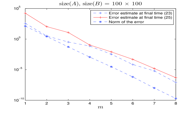
Fig. 1: Norm of the error vs number of Arnoldi iterations $m$

We observe that the bound (24) stated in Proposition 6 is slightly better in this example.

Next, we give another upper bound for the norm of the error ${\cal E}_{m}(t)$ .

Proposition 7.

Let $X(t)$ be the exact solution to (1) and let $X_{m}(t)$ be the approximate solution obtained at step $m$. Then we have

$$\|{\cal E}_{m}(t)\|\leq\|F\,\|e^{t\mu_{2}(B)}\,\Gamma_{1,m}(t)+\|E_{m}\,\|e^{t\mu_{2}(A)}\Gamma_{2,m}(t),$$ (27)

where

$$\Gamma_{1,m}(t)=\displaystyle\int_{t_{0}}^{t}e^{-\tau\mu_{2}(B)}\,\|Z_{A}(\tau)-Z_{m,A}(\tau)\|d\tau,\;\Gamma_{2,m}(t)=\displaystyle\int_{t_{0}}^{t}e^{-\tau\mu_{2}(A)}\|Z_{B}(\tau)-Z_{m,B}(\tau)\|d\tau.$$

Proof. From the expressions of $X(t)$ and $X_{m}(t)$, we have

$$\|{\cal E}_{m}(t)\|=\left\|\int_{t_{0}}^{t}\left(Z_{A}(\tau)Z_{B}(\tau)^{T}-Z_{m,A}(\tau)Z_{m,B}(\tau)^{T}\right)d\tau\right\|,$$ (28)

where $Z_{m,A}={\cal V}_{m}e^{(t-\tau)\mathcal{T}_{m,A}}E_{m}$, $Z_{m,B}(\tau)={\cal W}_{m}e^{(t-\tau)\mathcal{T}_{m,B}}F_{m}$, $Z_{A}(\tau)=e^{(t-\tau)A}E$ and $Z_{B}(\tau)=e^{(t-\tau)B}F$. Then, using the relation

$$Z_{A}(\tau)Z_{B}(\tau)^{T}-Z_{m,A}(\tau)Z_{m,B}(\tau)^{T}=(Z_{A}(\tau)-Z_{m,A}(\tau))Z_{B}^{T}+Z_{m,A}(\tau)(Z_{B}(\tau)-Z_{m,B}(\tau))^{T},$$

we obtain

$$\|Z_{A}(\tau)Z_{B}(\tau)^{T}-Z_{m,A}(\tau)Z_{m,B}(\tau)^{T}\| \leq \|Z_{B}(\tau)\|\,\|(Z_{A}(\tau)-Z_{m,A}(\tau))\|$$

$$+ \|Z_{m,A}(\tau)\|\,\|(Z_{B}(\tau)-Z_{m,B}(\tau))\|.$$

Now as $\|Z_{B}(\tau)\|\leq e^{(t-\tau)\mu_{2}(B)}\|F\|$ and since $\mu_{2}({\cal T}_{m,A})\leq\mu_{2}(A)$, we also have $\|Z_{m,A}(\tau)\|\leq e^{(t-\tau)\mu_{2}({\cal T}_{m,A})}\|E_{m}\|\leq e^{(t-\tau)\mu_{2}(A)}\|E_{m}\|$. Using all these relations in (28), we get

$$\|{\cal E}_{m}(t)\| \leq \int_{t_{0}}^{t}\left[e^{(t-\tau)\mu_{2}(B)}\|F\,\|Z_{A}(\tau)-Z_{m,A}(\tau)\|+e^{(t-\tau)\mu_{2}(A)}\|E_{m}\|\,\|Z_{B}(\tau)-Z_{m,B}(\tau)\|\right]d\tau$$

$$\leq \|F\,\|e^{t\mu_{2}(B)}\,\int_{t_{0}}^{t}e^{-\tau\mu_{2}(B)}\,\|Z_{A}(\tau)-Z_{m,A}(\tau)\|d\tau$$

$$+ \|E_{m}\,\|e^{t\mu_{2}(A)}\,\int_{t_{0}}^{t}e^{-\tau\mu_{2}(A)}\|(Z_{B}(\tau)-Z_{m,B}(\tau))\|d\tau,$$

which ends the proof.

One can use some known results [12, 16] to derive upper bounds for $\|Z_{A}(\tau)-Z_{m,A}(\tau)\|$ and $\|Z_{B}(\tau)-Z_{m,B}(\tau)\|$, when using Krylov or block Krylov subspaces. For general matrices $A$ and $B$, we can use the following result to get upper bounds for $\|Z_{A}(\tau)-Z_{m,A}(\tau)\|$ and $\|Z_{B}(\tau)-Z_{m,B}(\tau)\|$.

Proposition 8.

When using the extended block Arnoldi (or the block Arnoldi), we get the following upper bound for the exponential approximation error $e_{m,A}(\tau)=Z_{A}(\tau)-Z_{m,A}(\tau)$:

$$\|e_{m,A}(\tau)\|\leq\|T_{m+1,m}^{A}\|\int_{0}^{\tau}e^{(u-\tau)\nu(A)}\|L_{m,A}(u)\|du,$$ (29)

where $L_{m,A}(u)={\widetilde{E}}_{m}e^{(t-u){\cal T}_{m,A}}E_{m}$ and $\nu(A)=\lambda_{min}\left(\displaystyle\frac{A+A^{T}}{2}\right)$.

Proof. We have

$$Z_{A}(\tau)=e^{(t-\tau)A}E,\;\;{\rm and}\;\;Z_{m,A}(\tau)={\cal V}_{m}e^{(t-\tau){\cal T}_{m,A}}E_{m}.$$

Then ${Z^{\prime}_{A}}(\tau)=-Ae^{(t-\tau)A}E=-AZ_{A}(\tau)$, and

$${Z^{\prime}_{m,A}}(\tau)=-{\cal V}_{m}{\cal T}_{m,A}e^{(t-\tau){\cal T}_{m,A}}E_{m}=-[A{\cal V}_{m}-V_{m+1}T_{m+1,m}^{A}{\widetilde{E}}_{m}]e^{(t-\tau){\cal T}_{m,A}}E_{m}.$$

Hence,

$${Z^{\prime}_{m,A}}(\tau)=-AZ_{m,A}(\tau)+V_{m+1}T_{m+1,m}^{A}L_{m,A}(\tau),$$ (30)

where $L_{m,A}(\tau)={\widetilde{E}}_{m}e^{(t-\tau){\cal T}_{m,A}}E_{m}$.
Therefore, the error $e_{m,A}(\tau)=Z_{A}(\tau)-Z_{m,A}(\tau)$ is such that

$$e_{m,A}^{\prime}(\tau)=-Ae_{m}(\tau)-V_{m+1}T_{m+1,m}^{A}L_{m,A}(\tau),$$

which gives the following expression of $e_{m}$:

$$e_{m,A}(\tau)=-\displaystyle\int_{0}^{\tau}e^{(u-\tau)A}V_{m+1}T_{m+1,m}^{A}L_{m,A}(u)du.$$ (31)

On the other hand, since $\tau-u>0$, it follows that

$$\|e^{(u-\tau)A}\|\leq e^{(\tau-u)\mu_{2}(-A)}=e^{(u-\tau)\nu(A)}.$$

Then, we get

$$\|e_{m,A}(\tau)\|\leq\|T_{m+1,m}^{A}\|\int_{0}^{\tau}e^{(u-\tau)\nu(A)}\|L_{m,A}(u)\|du.$$

Notice that if $\nu(A)$ is not known but $\nu(A)\ \geq 0$ (which is the case for positive semidefinite matrices) then we get the upper bound

$$\|e_{m,A}(\tau)\|\leq\|T_{m+1,m}^{A}\|\int_{0}^{\tau}\|L_{m,A}(u)\|du.$$ (32)

To define a new upper bound for the norm of the global error ${\cal E}_{m}(t)$, we can use the upper bounds for the errors $e_{m,A}$ and $e_{m,B}$ in the expression (27) stated in Propostion 7 to get

$$\|{\cal E}_{m}(t)\| \leq \|F\,\|e^{t\mu_{2}(B)}\,\displaystyle\int_{t_{0}}^{t}e^{-\tau\mu_{2}(B)}\,\|e_{m,A}(\tau)\|d\tau$$

$$+ \|E_{m}\,\|e^{t\mu_{2}(A)}\displaystyle\int_{t_{0}}^{t}e^{-\tau\mu_{2}(A)}\|e_{m,B}(\tau)\|d\tau,$$

and then we obtain

$$\|{\cal E}_{m}(t)\| \leq \|F\,\|e^{t\mu_{2}(B)}\,\|T_{m+1,m}^{A}\|\displaystyle\int_{t_{0}}^{t}e^{-\tau\mu_{2}(B)}\,S_{m,A}(\tau)d\tau$$ (33)

$$+ \|E_{m}\,\|e^{t\mu_{2}(A)}\|T_{m+1,m}^{B}\|\displaystyle\int_{t_{0}}^{t}e^{-\tau\mu_{2}(A)}S_{m,B}(\tau)d\tau,$$ (34)

where $S_{m,A}(\tau)=\displaystyle\int_{0}^{\tau}e^{(u-\tau)\nu(A)}\|L_{m,A}(u)\|du$ and $S_{m,B}(\tau)=\displaystyle\int_{0}^{\tau}e^{(u-\tau)\nu(B)}\|L_{m,B}(u)\|du$.
As $m$ is generally very small as compared to $n$ and $p$, the factors $L_{m,A}$ and $L_{m,B}$ can be computed using Matlab fuctions such as expm and the integral appearing in the right sides of (29) and (33), can be approximated via a quadrature formulae.

We summarize the steps of our proposed first approach (using the extended block Arnoldi) in the following algorithm

Algorithm 1 The extended block Arnoldi (EBA-exp) method for DSE’s

• Input $X_{0}=X(t_{0})$, a tolerance $tol>0$, an integer $m_{max}$.

• For $m=1,\ldots,m_{max}$

  • Apply the extended block Arnoldi algorithm to $(A,E)$ and $(B^{T},F)$ to get the orthonormal matrices ${\mathcal{V}}_{m}=[V_{1},...,V_{m}]$ and ${\mathcal{W}}_{m}=[W_{1},...,W_{m}]$ and the upper block Hessenberg matrices ${\mathcal{T}}_{m,A}$ and ${\mathcal{T}}_{m,B}$.

  • Set ${E}_{m}={\mathcal{V}}_{m}^{T}E$, ${F}_{m}={\mathcal{W}}_{m}^{T}F$ and compute $Z_{m,A}(\tau)=e^{(t-\tau)\mathcal{T}_{m,A}}E_{m}$ and $Z_{m,B}(\tau)=e^{(t-\tau)\mathcal{T}_{m,B}}F_{m}$ using the matlab function expm.

  • Use a quadrature method to compute the integral (13) and get an approximation of $G_{m}(t)$ for each $t\in[t_{0},\,T_{f}]$.

  • If $\parallel R_{m}(t)\parallel=\displaystyle\max\{\parallel T_{m+1,m}^{A}{\bar{G}}_{m}(t)\parallel,\parallel T_{m+1,m}^{B}{\bar{G}}_{m}(t)\parallel\}<tol$ stop and compute the approximate solution $X_{m}(t)$ in the factored form given by the relation (19).

• End

3 Projecting and solving the low dimensional problem

3.1 Low-rank approximate solutions

In this section, we show how to obtain low rank approximate solutions to the differential Sylvester equation (1) by first projecting directly the initial problem onto block (or extended block) Krylov subspaces and then solve the obtained low dimensional differential problem. We first apply the block Arnoldi algorithm (or the extended block Arnoldi) to the pairs $(A,E)$ and $(B^{T},F)$ to get the orthonormal matrices ${\cal V}_{m}$ and ${\cal W}_{m}$, whose columns form orthonormal bases of the extended block Krylov subspaces ${\cal K}_{m}(A,E)$ and ${\cal K}_{m}(B^{T},F)$, respectively. We also get the upper block Hessenberg matrices ${\cal T}_{m,A}={\cal V}^{T}_{m}A{\cal V}_{m}$ and ${\cal T}_{m,B}={\cal W}^{T}_{m}B^{T}{\cal W}_{m}$.
Let $X_{m}(t)$ be the desired low rank approximate solution given as

$$X_{m}(t)={\cal V}_{m}Y_{m}(t){\cal W}_{m}^{T},$$ (35)

satisfying the Petrov-Galerkin orthogonality condition

$${\cal V}_{m}^{T}R_{m}(t){\cal W}_{m}=0,\;t\in[t_{0},\;T_{f}],$$ (36)

where $R_{m}(t)$ is the residual $R_{m}(t)=\displaystyle{\dot{X}}_{m}(t)-A\,X_{m}(t)-X_{m}(t)\,B-EF^{T}$. Then, from (35) and (36), we obtain the low dimensional differential Sylvester equation

$${\dot{Y}}_{m}(t)-{\cal T}_{m,A}\,Y_{m}(t)-Y_{m}(t)\,{\cal T}_{m,B}^{T}-E_{m}F_{m}^{T}=0,$$ (37)

where ${E}_{m}={\cal V}_{m}^{T}\,E$ and ${F}_{m}={\cal W}_{m}^{T}\,F$. The obtained low dimensional differential Sylvester equation (37) is the same as the one given by (14). We have now to solve the latter differential equation by some integration method such as the well known Backward Differentiation Method (BDF) [3] or the Rosenbrock method [3, 18].
Notice that all the properties and results such as the expressions of the residual norms or the upper bounds for the norm of the error given in the last section are still valid with this second approach. The two approaches only differ in the way the projected low dimensional differential Sylvester matrix equations are numerically solved.

3.2 BDF for solving the low order differential Sylvester equation (37)

We use the Backward Differentiation Formula (BDF) method for solving, at each step $m$ of the extended block Arnoldi (or block Arnoldi) process, the low dimensional differential Sylvester matrix equation (37). We notice that BDF is especially used for the solution of stiff differential equations.
At each time $t_{k}$, let $Y_{m,k}$ of the approximation of $Y_{m}(t_{k})$, where $Y_{m}$ is a solution of (37). Then, the new approximation $Y_{m,k+1}$ of $Y_{m}(t_{k+1})$ obtained at step $k+1$ by BDF is defined by the implicit relation

$$Y_{m,k+1}=\displaystyle\sum_{i=0}^{p-1}\alpha_{i}Y_{m,k-i}+h_{k}\beta{\mathcal{F}}(Y_{m,k+1}),$$ (38)

where $h_{k}=t_{k+1}-t_{k}$ is the step size, $\alpha_{i}$ and $\beta_{i}$ are the coefficients of the BDF method as listed in Table 1 and ${\mathcal{F}}(Y)$ is given by

$${\mathcal{F}}(Y)={\cal T}_{m,A}\,Y+Y\,{\cal T}_{m,B}^{T}+\,E_{m}\,F_{m}^{T}.$$

$p$	$\beta$	$\alpha_{0}$	$\alpha_{1}$	$\alpha_{2}$
1	1	1
2	2/3	4/3	-1/3
3	6/11	18/11	-9/11	2/11

Table 1: Coefficients of the $p$-step BDF method with $p\leq 3$.

The approximate $Y_{m,k+1}$ solves the following matrix equation

$$-Y_{m,k+1}+h_{k}\beta({\cal T}_{m,A}Y_{m,k+1}+Y_{m,k+1}{\cal T}_{m,B}^{T}+EF^{T})+\displaystyle\sum_{i=0}^{p-1}\alpha_{i}Y_{m,k-i}=0,$$

which can be written as the following Sylvester matrix equation

$$\mathbb{T}_{m,A}\,Y_{m,k+1}+\,Y_{m,k+1}\mathbb{T}_{m,B}^{T}+\mathbb{E}_{m,k}\,\mathbb{F}_{m,k}^{T}=0.$$ (39)

We assume that at each time $t_{k}$, the approximation $Y_{m,k}$ is factorized as a low rank product $Y_{m,k}\approx{\widetilde{U}}_{m,k}{{\widetilde{V}}_{m,k}}^{T}$, where ${\widetilde{U}}_{m,k}\in\mathbb{R}^{n\times m_{k}}$ and ${\widetilde{V}}_{m,k}\in\mathbb{R}^{p\times m_{k}}$, with $m_{k}\ll n,p$. In that case, the coefficient matrices appearing in (39) are given by

$$\mathbb{T}_{m,A}=h_{k}\beta{\cal T}_{m,A}-\displaystyle\frac{1}{2}I;\;\;\mathbb{T}_{m,B}=h_{k}\beta{\cal T}_{m,B}-\displaystyle\frac{1}{2}I,$$

$$\mathbb{E}_{m,k+1}=[\sqrt{h_{k}\beta}E^{T},\sqrt{\alpha_{0}}{\widetilde{U}}_{m,k}^{T},\ldots,\sqrt{\alpha_{p-1}}{\widetilde{U}}_{m,k+1-p}^{T}]^{T}\,$$

and

$$\mathbb{F}_{m,k+1}=[\sqrt{h_{k}\beta}F^{T},\sqrt{\alpha_{0}}{\widetilde{V}}_{m,k}^{T},\ldots,\sqrt{\alpha_{p-1}}{\widetilde{V}}_{m,k+1-p}^{T}]^{T}.$$

The Sylvester matrix equation (39) can be solved by applying direct methods based on Schur decomposition such as the Bartels-Stewart algorithm [2, 9].
Notice that we can also use the BDF method applied directly to the original problem (1) and then at each iteration, one has to solve large Sylvester matrix equations which can be done by using Krylov-based methods as developed in [6, 13].

3.3 Solving the low dimensional problem with the Rosenbrock method

Applying Rosenbrock method [3, 18] to the low dimensional differential Sylvester matrix equation (37), the new approximation $Y_{m,k+1}$ of $Y_{m}(t_{k+1})$ obtained at step $k+1$ is defined, in the ROS(2) particular case by the relations

$$Y_{m,k+1}=Y_{m,k}+\displaystyle\frac{3}{2}K_{1}+\frac{1}{2}K_{2},$$ (40)

where $K_{1}$ and $K_{2}$ solve the following Sylvester equations

$$\widetilde{\mathbb{T}}_{m,A}K_{1}+K_{1}\widetilde{\mathbb{T}}_{m,B}=-\mathcal{F}(t_{k},Y_{m,k}),$$ (41)

and

$$\widetilde{\mathbb{T}}_{m,A}K_{2}+K_{2}\widetilde{\mathbb{T}}_{m,B}=-\mathcal{F}(t_{k+1},Y_{m,k}+K_{1})+\displaystyle\frac{2}{h}K_{1},$$ (42)

where

$$\widetilde{\mathbb{T}}_{m,A}=\gamma{\mathcal{T}}_{m,B}-\displaystyle\frac{1}{2h}I\;\;{\rm and}\;\;\widetilde{\mathbb{T}}_{m,B}=\gamma{\mathcal{T}}_{m,B}^{T}-\displaystyle\frac{1}{2h}I,$$

and

$$\mathcal{F}(Y)={\mathcal{T}}_{m,A}Y+Y{\mathcal{T}}_{m,B}^{T}+E_{m}F_{m}^{T}.$$

We summarize the steps of the second approach (using the extended block Arnoldi) in the following algorithm

Algorithm 2 The extended block Arnoldi (EBA) method for DSE’s

• Input $X_{0}=X(t_{0})$, a tolerance $tol>0$, an integer $m_{max}$.

• For $m=1,\ldots,m_{max}$

  • Apply the extended block Arnoldi algorithm to the pairs $(A,E)$ and $(B^{T},F)$ to compute the orthonormal bases ${\mathcal{V}}_{m}=[V_{1},...,V_{m}]$ and ${\mathcal{W}}_{m}=[W_{1},...,W_{m}]$ and also the the upper block Hessenberg matrices ${\mathcal{T}}_{m,A}$ and ${\mathcal{T}}_{m,B}$.

  • Use the BDF or the Rosenbrock method to solve the low dimensional differential Sylvester equation

    $${\dot{Y}}_{m}(t)-{\cal T}_{m,A}\,Y_{m}(t)-Y_{m}(t)\,{\cal T}_{m,B}^{T}-E_{m}F_{m}^{T}=0,\;t\in[t_{0},\,T_{f}]$$

  • If $\parallel R_{m}(t)\parallel<tol$ stop and compute the approximate solution $X_{m}(t)$ in the factored form given by the relation (19).

• End

4 Numerical examples

In this section, we compare the approaches presented in this paper. The exponential approach (EBA-exp) summarized in Algorithm 1, which is based on the approximation of the solution to (1) applying a quadrature method to compute the projected exponential form solution (13). We used a scaling and squaring strategy, implemented in the MATLAB expm function; see [11, 14] for more details. The second method (Algorithm 2) is based on the BDF integration method applied to the projected Sylvester equation as described in Section (3.2). Finally, we considered the EBA-ROS(2) method as described in Section (3.3). The basis of the projection subspaces were generated by the extended block Arnoldi algorithm for all methods. All the experiments were performed on a laptop with an Intel Core i7 processor and 8GB of RAM. The algorithms were coded in Matlab R2014b.

Example 1. For this example, the matrices $A\in\mathbb{R}^{n\times n}$ and $B\in\mathbb{R}^{p\times p}$ were obtained from the 5-point discretization of the operators

$${L_{A}=\Delta u-f_{1}(x,y)\frac{\partial u}{\partial x}+f_{2}(x,y)\frac{\partial u}{\partial y}+g_{1}(x,y)},$$

and

$${L_{B}=\Delta u-f_{3}(x,y)\frac{\partial u}{\partial x}+f_{4}(x,y)\frac{\partial u}{\partial y}+g_{2}(x,y)},$$

on the unit square $[0,1]\times[0,1]$ with homogeneous Dirichlet boundary conditions. The number of inner grid points in each direction are $n_{0}$ for $A$ and $p_{0}$ for $B$ and the dimension of the matrices $A$ and $B$ are $n=n_{0}^{2}=$ and $p=p_{0}^{2}$ respectively. Here we set $f_{1}(x,y)=x+10y^{2}$, $\displaystyle{f_{2}(x,y)=\sqrt{2x^{2}+y^{2}}}$, $f_{3}(x,y)=x+2y$, $f_{4}(x,y)=exp(y-x)$ , $g_{1}(x,y)=x^{2}-y^{2}$ and $g_{2}(x,y)=y^{2}-x^{2}$. The time interval considered was $[0,\,2]$ and the initial condition $X_{0}=X(0)$ was $X_{0}=Z_{0}Z_{0}^{T}$, where $Z_{0}=0_{n\times 2}$.

For all projection-based methods, we used projections onto the Extended Block Krylov subspaces ${\mathcal{K}}_{k}(A,B)={\rm Range}(B,A\,B,\ldots,A^{m-1}\,B,A^{-1}\,B,\ldots,(A^{-1})^{m}\,B)$ and the tolerance was set to $10^{-10}$ for the stop test on the residual. For the EBA-BDF and Rosenbrock methods, we used a constant timestep $h$. The entries of the matrices $E$ and $F$ were random values uniformly distributed on the interval $[0,\,1]$ and their rank were set to $s=2$.
To the authors’ knowledge, there are no available exact solutions of large scale matrix Sylvester differential equations in the literature. In order to check if our approaches produce reliable results, we first compared our results to the one given by Matlab’s ode23s solver which is designed for stiff differential equations. This was done by vectorizing our DSE, stacking the columns of $X$ one on top of each other. This method is not suited to large-scale problems. Due to the memory limitation of our computer when running the ode23s routine, we chose a size of $100\times 100$ for the matrices $A$ and $B$.
In Figure 2, we compared the component $X_{11}$ of the solution obtained by the methods tested in this section, to the solution provided by the ode23s method from Matlab, on the time interval $[0,\,2]$, for $size(A),~{}size(B)=100\times 100$ and a constant timestep $h=10^{-2}$. We observe that all the considered methods give good results in terms of accuracy. The relative error norms at final time $T_{f}=2$ were of order $\mathcal{O}(10^{-10})$ for the EBA-exp method and $\mathcal{O}(10^{-12})$ for the others. The runtimes were respectively 0.6s for EBA-exp, 7.3s for EBA-BDF(1), 20.8s for EBA-BDF(2) and 29.2s for EBA-ROS(2). The ode23s routine required 978s.

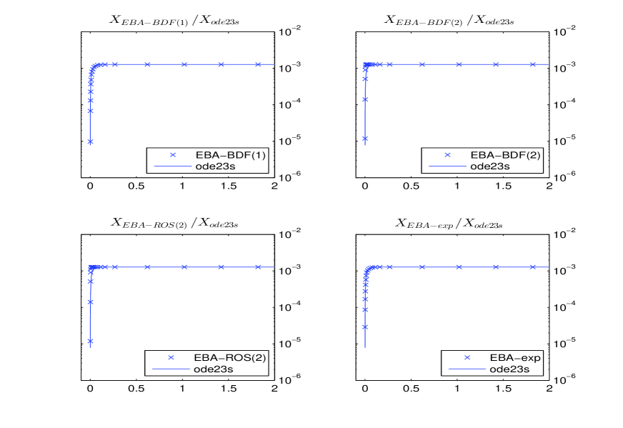
Fig. 2: Values of $X_{11}(t)$ for $t\in[0,\,2]$

In Table 2, we give the obtained runtimes in seconds, the number of Arnoldi iterations and the Frobenius residual norm at final time, for the resolution of Equation (1) for $t\in[0,\,2]$, with a timestep $h=0.01$.

	EBA-exp	EBA-BDF(1)	EBA-BDF(2)	EBA-ROS(2)
$n,p=2500,2500$	$3.8$s $(m=16)$	$6.1$s $(m=18)$	$13.6$s $(m=18)$	$28.8$s $(m=23)$
$\|R_{m}(T_{f})\|_{F}$	$1.04\times 10^{-8}$	$2.45\times 10^{-10}$	$2.45\times 10^{-10}$	$3.05\times 10^{-10}$
$n,p=10000,10000$	$35.2$s $(m=22)$	$38.4$s $(m=25)$	$80.3$s $(m=25)$	$104.7$s $(m=33)$
$\|R_{m}(T_{f})\|_{F}$	$4.4\times 10^{-9}$	$4.1\times 10^{-11}$	$4.2\times 10^{-11}$	$5.8\times 10^{-11}$
$n,p=22500,10000$	$137.3$s $(m=22)$	$166.5$s $(m=30)$	$342.3$s $(m=30)$	$246$s $(m=35)$
$\|R_{m}(T_{f})\|_{F}$	$4.2\times 10^{-8}$	$3.7\times 10^{-11}$	$3.6\times 10^{-11}$	$1.78\times 10^{-9}$

Table 2: Runtimes in seconds and the residual norms

The results in Table 2 show that the EBA-exp method is outperformed by the other approaches in terms of accuracy, although it allows to obtain an acceptable approximation more quickly. The EBA-BDF(1) appears to be the better option in terms of time and accuracy.

Example 2 In this second example, we considered the particular case

$$\left\{\begin{array}[]{l}\dot{X}(t)=A(t)\,X(t)+X(t)\,A(t)-E(t)F(t)^{T};\;(DSE)\\ \;X(t_{0})=X_{0},\;\;t\in[t_{0},\,T_{f}],\end{array}\right.$$ (43)

where the matrix $A=Rail1357$ was extracted from the IMTEK collection Optimal Cooling of Steel Profiles . We compared the EBA-BDF(1) method to the EBA-exp and EBA-ROS(2) methods for the problem size $n=1357$ on the time interval $[0\,,2]$. The initial value $X_{0}$ was chosen as $X_{0}=0$ and the timestep was set to $h=0.001$. The tolerance for EBA stop test was set to $10^{-7}$ for all methods and the projected low dimensional Sylvester equations were numerically solved by the solver (lyap from Matlab at each iteration of the extended block Arnoldi algorithm for the EBA-BDF(1), EBA-BDF(2) and EBA-ROS(2) methods. As the size of the coefficient matrices allowed it, we also computed an approximate solution of (43) applying a quadrature method to the integral form of the exact solution given by Formula(4) and took it as a reference solution. In Table 3, we reported the runtimes, in seconds, the number $m$ of Arnoldi iterations and the Frobenius norm $\|\mathcal{E}(T_{f})_{m}\|_{F}$ of the error at final time.

	EBA-exp	EBA-BDF(1)	EBA-BDF(2)	EBA-ROS(2)
Runtime (s)	$48.4$ s ($m=18$)	$471.9$ s ($m=18)$	$1549.2$s ($m=23$)	$1827$s ($m=21$)
$\|\mathcal{E}_{m}(T_{f})\|_{F}$	$1.28\times 10^{-10}$	$5\times 10^{-5}$	$1.48\times 10^{-4}$	$4.9\times 10^{-5}$.

Table 3: Optimal Cooling of Steel Profiles: runtimes, number of Arnoldi iterations and error norms

As can be seen from the reported results in Table 3, the EBA-exp method clearly outperforms all the other listed options.

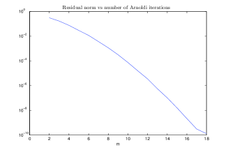
Fig. 3: Residual norm vs number $m$ of Arnoldi iterations

In Figure (3), we plotted the Frobenius residual norm $\|R_{m}(t_{f})\|_{F}$ at final time $T_{f}$ in function of the number $m$ of Arnoldi iterations for the EBA-exp method.

5 Appendix A

Here we recall the extended block Arnoldi (EBA) and block Arnoldi (BA) algorithms, when applied to the pair $(A,E)$. EBA is described in Algorithm 3 as follows

Algorithm 3 The extended block Arnoldi algorithm (EBA)

• Inputs: $A$ an $n\times n$ matrix, $E$ an $n\times s$ matrix and $m$ an integer.

• Compute the QR decomposition of $[E,A^{-1}E]$, i.e., $[E,A^{-1}E]=V_{1}\Lambda$;
              Set ${\mathcal{V}}_{0}=\left[~{}\right]$;

• For $j=1,\ldots,m$

• Set $V_{j}^{(1)}$: first $s$ columns of $V_{j}$ and $V_{j}^{(2)}$: second $s$ columns of $V_{j}$

• ${\mathcal{V}}_{j}=\left[{\mathcal{V}}_{j-1},V_{j}\right]$; $\hat{V}_{j+1}=\left[A\,V_{j}^{(1)},A^{-1}\,V_{j}^{(2)}\right]$.

• Orthogonalize $\hat{V}_{j+1}$ w.r.t ${\mathcal{V}}_{j}$ to get $V_{j+1}$, i.e.,
                   For $i=1,2,\ldots,j$
                        $H_{i,j}=V_{i}^{T}\,\hat{V}_{j+1}$;
                        $\hat{V}_{j+1}=\hat{V}_{j+1}-V_{i}\,H_{i,j}$;
                   Endfor $i$

• Compute the QR decomposition of $\hat{V}_{j+1}$, i.e., $\hat{V}_{j+1}=V_{j+1}\,H_{j+1,j}$.
  

• Endfor $j$.

The block Arnoldi algorithm is summarized in Algorithm 4 as follows

Algorithm 4 The block Arnoldi algorithm (BA)

• Inputs: $A$ an $n\times n$ matrix, $E$ an $n\times s$ matrix and $m$ an integer.

• Compute the QR decomposition of $E$, i.e., $E=V_{1}R_{1}$.

• For $j=1,\ldots,m$

  1. $W_{j}=AV_{j}$,

  2. for $i=1,2,\ldots,j$

     • $H_{i,j}=V_{i}^{T}\,W_{j},$

     • $W_{j}=W_{j}-V_{j}\,H_{i,j},$

  3. endfor

  4. $Q_{j}R_{j}=W_{j}$ ($QR$ decomposition)

  5. $V_{j+1}=Q_{j}$, and $H_{j+1,j}=R_{j}$.

• EndFor $j$

Since the above algorithms implicitly involve a Gram-Schmidt process, the obtained blocks ${\cal V}_{m}=\left[V_{1},V_{2},\ldots,V_{m}\right]$ ($V_{i}\in\mathbb{R}^{n\times d}$) ,where $d=s$ for the block Arnoldi and $d=2s$ for the extended block Arnoldi, have their columns mutually orthogonal provided none of the upper triangular matrices $H_{j+1,j}$ are rank deficient. Hence, after $m$ steps, Algorithm 3 and Algorithm 4 build orthonormal bases ${\cal V}_{m}$ of the Krylov subspaces ${\cal K}_{m}(A,E)={\rm Range}(E,A\,E,\ldots,A^{m-1}\,E,A^{-1}\,E,\ldots,(A^{-1})^{m}\,E)$ or $\mathbb{K}_{m}(A,E)={\rm Range}(E,A\,E,\ldots,A^{m-1}\,E)$, respectively and a block upper Hessenberg matrix ${\cal H}_{m}$ whose nonzero sub-blocks are the $H_{i,j}$. Note that each submatrix $H_{i,j}$ ($1\leq i\leq j\leq m$) is of order $d$.
Let ${\cal T}_{m}\in\mathbb{R}^{d\times d}$ be the restriction of the matrix $A$ to the extended Krylov subspace ${\cal K}_{m}(A,E)$ (or to the block Krylov subspace $\mathbb{K}_{m}(A,E)$), i.e., ${\cal T}_{m}={\cal V}_{m}^{T}\,A\,{\cal V}_{m}$. Then it can be shown that matrix ${\cal T}_{m}$ is also block upper Hessenberg with $d\times d$ blocks, see[10, 17] . For the block Arnoldi algorithm, ${\cal T}_{m}={\cal H}_{m}$ while for the extended block Arnoldi algorithm, a recursion can be derived to compute ${\cal T}_{m}$ from ${\cal H}_{m}$ without requiring matrix-vector products with $A$, see [17]. We notice that for large and non structured problems, the inverse of the matrix $A$ is not computed explicitly and in this case we can use iterative solvers with preconditioners to solve linear systems with $A$.

6 Conclusion

We presented in the present paper two new approaches for computing approximate solutions to large scale differential Sylvester matrix equations. The first one comes naturally from the exponential expression of the exact solution and the use of approximation techniques of the exponential of a matrix times a block of vectors. The second approach is obtained by first projecting the initial problem onto a block Krylov (or extended Krylov) subspace, obtain a low dimensional differential Sylvester equation which is solved by using the well known BDF or Rosenbrock integration method. We gave some theoretical results such as the exact expression of the residual norm and also upper bounds for the norm of the error. Numerical experiments show that both approaches are promising for large-scale problems, with a clear advantage for the EBA-exp method in terms of computation time although the EBA-BDF(1) method shows to offer a good balance between the execution time and the accuracy in some cases.

References

[1]H. Abou-Kandil, G. Freiling, V. Ionescu, G. Jank, Matrix Riccati Equations in Control and Sytems Theory, in Systems & Control Foundations & Applications, Birkhauser, (2003).
[2]R.H. Bartels, G.W. Stewart, Algorithm 432:
Solution of the matrix equation AX+XB=C, Circ. Syst. Signal
Proc., 13 (1972), 820–826.
[3]J.C. Butcher, Numerical Methods for Ordinary Differential Equations, John Wiley & Sons, 2008
[4]M. J. Corless and A. E. Frazho, Linear systems and control - An operator perspective, Pure and Applied Mathematics. Marcel Dekker, New York-Basel, 2003.
[5]V. Druskin, L. Knizhnerman, Extended Krylov subspaces: approximation of the matrix square root and related functions, SIAM J. Matrix Anal. Appl., 19(3)(1998), 755–771.
[6]A. El Guennouni, K. Jbilou and A.J. Riquet, Block Krylov subspace methods for solving large Sylvester equations, Numer. Alg., 29 (2002), 75–96.
[7]E. Gallopoulos and Y. Saad, Efficient solution of parabolic equations by Krylov approximation methods, SIAM J. Sci. Statist. Comput., 13 (1992), 1236–1264.
[8]K. Glover, All optimal Hankel-norm approximations of linear multivariable systems and their L-infinity error bounds. International Journal of Control, 39(1984) 1115–1193.
[9]G.H. Golub, S. Nash and C. Van Loan, A Hessenberg Schur method for the problem , IEEE Trans. Automat. Contr., 24 (1979), 909–913.‘
[10]M. Heyouni, K. Jbilou, An Extended Block Arnoldi algorithm for Large-Scale Solutions of the Continuous-Time Algebraic Riccati Equation, Electronic Transactions on Numerical Analysis, 33, 53–62, (2009).
[11]N. J. Higham, The scaling and squaring method for the matrix
exponential revisited. SIAM J. Matrix Anal. Appl., 26(4) (2005), 1179-1193.
[12]
M. Hochbruck and C. Lubich, On Krylov subspace approximations to the matrix exponential
operator, SIAM J. Numer. Anal., 34 (1997), 1911–1925.
[13]K. Jbilou, Low-rank approximate solution to large Sylvester matrix equations, App. Math. Comput., 177 (2006), 365–376.
[14]C.B. Moler, C.F. Van Loan, Nineteen Dubious Ways to Compute the Exponential of a Matrix, SIAM Review 20, 1978, pp. 801–836. Reprinted and updated as ”Nineteen Dubious Ways to Compute the Exponential of a Matrix, Twenty-Five Years Later,” SIAM Review 45(2003), 3–49.
[15]Y. Saad, Numerical solution of large Lyapunov
equations,
in Signal Processing, Scattering, Operator Theory and Numerical Methods.
Proceedings of the international symposium MTNS-89, vol. 3, M.A.
Kaashoek, J.H. van Schuppen and A.C. Ran, eds., Boston, 1990,
Birkhauser, pp. 503–511.
[16]Y. Saad, Analysis of some Krylov subspace approximations to the matrix exponential operator,
SIAM J. Numer. Anal., 29 (1992), 209–228.
[17]V. Simoncini, A new iterative method for solving large-scale Lyapunov matrix equations, SIAM J. Sci. Comp., 29(3) (2007), 1268–1288.
[18]Rosenbrock H. H.Some general implicit processes for the numerical solution
of differential equations, J. Comput. , 5(1963), 329?330.
[19]H. van der Vorst, Iterative Krylov Methods for Large Linear Systems, Cambridge University
Press, Cambridge, 2003.