Computing All Border Bases for Ideals of Points

Abstract.

In this paper we consider the problem of computing all possible order ideals and also sets connected to $1$, and the corresponding border bases, for the vanishing ideal of a given finite set of points. In this context two different approaches are discussed: based on the Buchberger-Möller Algorithm [14], we first propose a new algorithm to compute all possible order ideals and the corresponding border bases for an ideal of points. The second approach involves adapting the Farr-Gao Algorithm [5] for finding all sets connected to $1$, as well as the corresponding border bases, for an ideal of points. It should be noted that our algorithms are term ordering free. Therefore they can compute successfully all border bases for an ideal of points. Both proposed algorithms have been implemented and their efficiency is discussed via a set of benchmarks.

1. Introduction

The theory of border bases is a fundamental tool in computational commutative algebra. These bases have been developed mainly for zero-dimensional ideals. In this case we can consider them as a generalization of Gröbner bases, introduced by B. Buchberger in his PhD thesis [4], which focuses on the structure of the quotient algebra. More precisely, border basis theory provides a way to find a structurally stable monomial basis for a zero-dimensional quotient ring of the polynomial ring, and it yields a special generating set for the ideal, called a border basis. For particular choices of the monomial basis, the border basis contains a reduced Gröbner basis of the ideal.

Since border bases have been shown to provide good numerical stability (e.g., see [18] and [10]), they have been explored to study zero-dimensional systems with approximate coefficients obtained from empirical measurements. Several algorithms have been designed for computing border bases, for instance the algorithm presented in [8] and implemented in the ApCoCoA computer algebra system (cf. [19]). Border bases of zero-dimensional polynomial ideals have turned out to be a powerful tool in computer algebra. They have been employed to solve many important problems in different fields of mathematics, including linear programming, logic, coding theory, and statistics. Many authors have worked on this topic, starting from the initial papers by M.G. Marinari, M. Möller and T. Mora [13] as well as by W. Auzinger and H.J. Stetter [2], continuing with the contributions by B. Mourrain [15], A. Kehrein and M. Kreuzer [8], as well as B. Mourrain and P. Trébuchet [16], and a first textbook chapter in [12]. Furthermore, B. Mourrain and P. Trébuchet generalized in [15, 16, 17] the notion of order ideals to sets connected to $1$ which we shall call quasi order ideals (see Section 2). Based on this definition, they studied a generalized version of border bases, which we shall call quasi border bases, and their application to solving polynomial systems. For more details on border bases, we refer to Section 6.4 in [12].

Given a finite set of points, finding the ideal consisting of all polynomials vanishing on it, the so-called vanishing ideal of the set of points, has numerous applications both inside and outside of Mathematics, for example in statistics, optimization, computational biology, and coding theory. Therefore many authors have been interested in studying different aspects of computing vanishing ideals of finite sets of points. In 1982, B. Buchberger and M. Möller proposed in [14] the first specialized algorithm to compute a Gröbner basis for the vanishing ideal of a set of given points. This algorithm proceeds by performing Gaussian elimination on a generalized Vandermonde matrix, and it has a polynomial time complexity. In 2006, J.B. Farr and S. Gao presented in [5] an incremental algorithm to compute a Gröbner basis for the vanishing ideal of a set of points. However, both of these algorithms are numerically unstable. To address this problem, in [1, 6] the authors presented numerically stable algorithms to compute a border basis for an ideal of points, as well as its application to industrial problems.

This leads us to the main topic of this paper, namely to calculate all order ideals, and also all quasi order ideals, as well as the corresponding border bases, for an ideal of points. Keep in mind that all traditional algorithms to compute border bases rely on degree-compatible term orderings, but a zero-dimensional ideal has border bases with respect to many order ideals which cannot derived from a term ordering. Let us review some previous results in this direction. In 2013, S. Kaspar weakened in [7] the term ordering requirement by introducing a term marking strategy and proposed an algorithm which computes border bases which cannot be obtained by following a term ordering strategy (see the following example). However, he did not provide any algorithm to find all such bases. Later, in [3], G. Braun and S. Pokutta used polyhedral theory and adapted the classical border basis algorithm to calculate all border bases for an ideal of points.

Let us exhibit an example from [7] which shows that there exists a border basis which cannot be obtained by any algorithm based on a term ordering strategy or the algorithm by G. Braun and S. Pokutta. Let $\mathbb{X}$ be the finite set of points $\{(1,1),(-1,1),(0,0),(1,0),(0,-1)\}$ in $\mathbb{Q}^{2}$. Then the set $\{1,y,y^{2},x,x^{2}\}$ is an order ideal for which the vanishing ideal of $\mathbb{X}$ has a border basis, namely $\{xy+x^{2}-1/2y^{2}-x-1/2y$, $x^{3}-x$, $x^{2}y-1/2y^{2}-1/2y,\,xy^{2}+x^{2}-1/2y^{2}-x-1/2y,\,y^{3}-y\}$. We note that, if we consider any term ordering, then the leading term of the first polynomial is either $x^{2}$ or $y^{2}$. However both terms belong to the order ideal. Based on the Buchberger-Möller Algorithm (see [14]) and the Farr-Gao Algorithm (see [5]), we propose two different novel algorithms to compute, respectively, all order ideals and all quasi order ideals, and also the corresponding border bases, for an ideal of points. We have implemented both algorithms in Maple and ApCoCoA (cf. [19]). Their efficiency is discussed via several explicit examples.

The rest of the paper is organized as follows. In the next section we recall basic notations and definitions. In Sections $3$ and $4$ we discuss our novel approaches based on the Buchberger-Möller Algorithm (resp. the Farr-Gao Algorithm) to compute all order ideals (resp. all quasi order ideals) for which a given ideal of points has a border basis (resp. a quasi border basis). Furthermore, we illustrate the proposed algorithms with some basic examples. The efficiency of the algorithms is discussed in Section $5$ via a set of benchmarks.

2. Preliminaries

In this section we give a brief review of basic definitions and results relating to Gröbner bases and border bases which will be used in the next sections. For further details we refer the reader to [12], Section 6.4.

Throughout this paper we let $\mathbbm{k}$ be a field, let $\mathcal{R}=\mathbbm{k}[x_{1},\ldots,x_{n}]$, and let $\mathcal{T}$ be the set of all terms in $x_{1},\ldots,x_{n}$, i.e.,

$\mathcal{T}=\{x_{1}^{\alpha_{1}}\cdots x_{n}^{\alpha_{n}}\mid\alpha_{i}\geq 0,\,1\leq i\leq n\}.$

Here we assume that $\prec$ is a term ordering on $\mathcal{T}$, i.e., a total ordering on $\mathcal{T}$ which is multiplicative and a well-ordering. For a polynomial $f\in\mathcal{R}\setminus\{0\}$, we define its leading term, denoted by $\operatorname{LT}(f)$, to be the greatest term with respect to $\prec$ which occurs in $f$. Given an ideal $\mathcal{I}\subset\mathcal{R}$, we denote by $\operatorname{LT}(\mathcal{I})$ the ideal generated by all $\operatorname{LT}(f)$ with $f\in\mathcal{I}\setminus\{0\}$. For a finite set $F=\{f_{1},\ldots,f_{k}\}\subset\mathcal{R}$, we write $\operatorname{LT}(F)$ for the set $\{\operatorname{LT}(f_{1}),\ldots,\operatorname{LT}(f_{k})\}$. A finite set $G\subset\mathcal{R}$ is called a Gröbner basis for $\mathcal{I}$ w.r.t. $\prec$ if $G\subset\mathcal{I}$ and $\operatorname{LT}(\mathcal{I})=\langle\operatorname{LT}(g)\ |\ g\in G\rangle$.

Definition 2.1.

Let $\mathcal{O}$ be a finite subset of $\mathcal{T}$.

1. The set $\mathcal{O}$ is called an order ideal  if it is closed under divisors, i.e., $t^{\prime}\in\mathcal{O}$ and $t\mid t^{\prime}$ imply $t\in\mathcal{O}$ for all $t,t^{\prime}\in\mathcal{T}$.

2. Given an order ideal $\mathcal{O}\subset\mathcal{T}$ and an ideal $\mathcal{I}\subset\mathcal{R}$, we say that $\mathcal{I}$ supports an $\mathcal{O}$-border basis if the residue classes of the terms in $\mathcal{O}$ form a basis of $\mathcal{R}/\mathcal{I}$ as a $\mathbbm{k}$-vector space.

3. If $\mathcal{O}\subset\mathcal{T}$ is an order ideal, the set $\partial\mathcal{O}=(x_{1}\mathcal{O}\cup\cdots\cup x_{n}\mathcal{O})\setminus\mathcal{O}$ is called the border of $\mathcal{O}$. For the empty order ideal, we define $\partial\mathcal{O}:=\{1\}$.

Example 2.2.

Consider the order ideal $\mathcal{O}=\{1,x,y,xy,x^{2},y^{2}\}$ in $\mathbbm{k}[x,y]$. Then the border of $\mathcal{O}$ is given by $\partial\mathcal{O}=\{x^{3},x^{2}y,xy^{2},y^{3}\}$. We illustrate $\mathcal{O}$ and its border in the following figure.

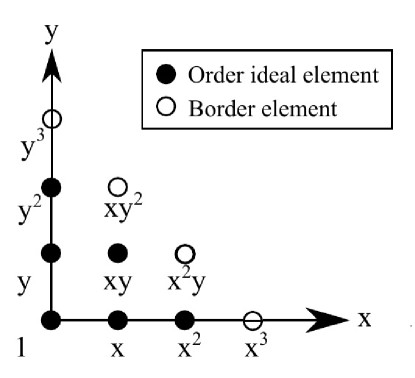
Figure 1. Depiction of an order ideal and its border

Definition 2.3.

Let $\mathcal{O}=\{t_{1},\ldots,t_{\mu}\}\subset\mathcal{T}$ be an order ideal and $\partial\mathcal{O}=\{b_{1},\ldots,b_{\nu}\}$.

1. A set of polynomials $G=\{g_{1},\ldots,g_{\nu}\}\subset\mathcal{R}$ is called an $\mathcal{O}$-border prebasis if every $g_{j}$ has the form

   $g_{j}=b_{j}-\sum_{i=1}^{\mu}\alpha_{ij}t_{i}$

   where $\alpha_{ij}\in\mathbbm{k}$.

2. If a polynomial $f\in\mathcal{R}\setminus\{0\}$ has the form $f=b_{j}-\sum_{i}c_{ij}t_{i}$ with $c_{ij}\in\mathbbm{k}$, $t_{i}\in\mathcal{O}$ and $b_{j}\in\partial\mathcal{O}$, we say that $f$ is in $\mathcal{O}$-border prebasis shape.

3. Let $\mathcal{I}\subset\mathcal{R}$ be a zero-dimensional ideal, and let $G=\{g_{1},\ldots,g_{\nu}\}$ be an $\mathcal{O}$-border prebasis. Then $G$ is called an $\mathcal{O}$-border basis of $\mathcal{I}$ if $G\subset\mathcal{I}$ and the residue classes of the elements of $\mathcal{O}$ form a $\mathbbm{k}$-vector space basis of $\mathcal{R}/\mathcal{I}$. In this case, the pair $(\mathcal{O},G)$ will be called a border pair for $\mathcal{I}$.

Example 2.4.

Let $\mathcal{R}=\mathbbm{k}[x,y]$ and $\mathcal{I}=\langle x^{2}+2y,y^{2}-3xy+4\rangle$. The set $\mathcal{O}=\{1,x,y,xy\}$ is an order ideal and we have $\partial\mathcal{O}=\{x^{2},y^{2},x^{2}y,xy^{2}\}$. It is easy to check that the set $G=\{y^{2}-3xy+4,x^{2}+2y,xy^{2}+18xy+4x-24,x^{2}y+6xy-8\}$ is an $\mathcal{O}$-border basis of $\mathcal{I}$.

In theory of border bases, we also use the concept of a border form which is defined as follows.

Definition 2.5.

Let $\mathcal{O}=\{t_{1},\ldots,t_{\mu}\}$ be an order ideal in $\mathcal{T}$.

1. For every $t^{\prime}\in\mathcal{T}$, let $k\geq 0$ be the least number such that there exists an index $i\in\{1,\dots,\mu\}$ and a term $t^{\prime\prime}$ of degree $k$ such that $t^{\prime}=t_{i}\,t^{\prime\prime}$. The number $k$ is called the index of $t^{\prime}$ w.r.t. $\mathcal{O}$ and denoted by $\operatorname{ind}_{\mathcal{O}}(t^{\prime})$.

2. For a polynomial $f\in\mathcal{R}\setminus\{0\}$, we let $\operatorname{ind}_{\mathcal{O}}(f)$ be the largest index of a term in its support. Write $f=c_{1}t^{\prime}_{1}+\cdots+c_{s}t^{\prime}_{s}$ with $c_{i}\in\mathbbm{k}$ and $t^{\prime}_{i}\in\mathcal{T}$. Then $\operatorname{BF}_{\mathcal{O}}(f)=\sum_{\{i\mid\operatorname{ind}(t^{\prime}_{i})=\operatorname{ind}(f)\}}c_{i}t^{\prime}_{i}$ is called the border form of $f$.

3. For a polynomial $f=b_{j}-\sum_{i}c_{ij}t_{i}\in\mathcal{R}\setminus\{0\}$, in $\mathcal{O}$-border prebasis shape the term $b_{j}$ is also called the border term of $f$ and denoted by $\operatorname{BT}_{\mathcal{O}}(f)$. Also, if $G$ is a set of polynomials whose elements are in $\mathcal{O}$-border prebasis shape, we denote the set $\{\operatorname{BT}_{\mathcal{O}}(g)\mid g\in G\}$ by $\operatorname{BT}_{\mathcal{O}}(G)$.

For some properties of the border form, we refer to [12], Section 6.4. Mourrain [15] introduced a generalization of order ideals, namely sets connected to $1$. Instead, for more homogeneity, we call them quasi order ideals. They are defined as follows.

Definition 2.6.

Let $\mathcal{O}$ be a finite subset of $\mathcal{T}$.

1. The border $\partial\mathcal{O}$ of $\mathcal{O}$ is defined by $\partial\mathcal{O}=(x_{1}\mathcal{O}\cup\cdots\cup x_{n}\mathcal{O})\setminus\mathcal{O}$.

2. The set $\mathcal{O}$ is called a quasi order ideal if for every $t\in\mathcal{O}\setminus\{1\}$ we have $t\in\partial(\mathcal{O}\setminus\{t\})$. Also, we define $\widehat{\mathcal{O}}=\mathcal{O}\cup\partial\mathcal{O}$.

3. Given an ideal $\mathcal{I}$ in $\mathcal{R}$ and a quasi order ideal $\mathcal{O}$, we say that $\mathcal{I}$ supports a quasi $\mathcal{O}$-border basis if the residue classes of the terms in $\mathcal{O}$ form a basis of $\mathcal{R}/\mathcal{I}$ as a $\mathbbm{k}$-vector space.

4. Let $\mathcal{O}=\{t_{1},\ldots,t_{\mu}\}$ be a quasi order ideal and $\partial\mathcal{O}=\{b_{1},\ldots,b_{\nu}\}$ its border. Then a set of polynomials $G=\{g_{1},\ldots,g_{\nu}\}$ in $\mathcal{R}$ is called a quasi $\mathcal{O}$-border prebasis of $\mathcal{I}$ if $G\subset\mathcal{I}$ and if, for every $j\in\{1,\dots,\nu\}$, we have $g_{j}=b_{j}-\sum_{i=1}^{\mu}\alpha_{ij}t_{i}$ where $\alpha_{ij}\in\mathbbm{k}$. Also, if a polynomial $f\in\mathcal{R}\setminus\{0\}$ has the form $f=b_{j}-\sum_{i}c_{ij}t_{i}$ with $c_{ij}\in\mathbbm{k}$, $t_{i}\in\mathcal{O}$ and $b_{j}\in\partial\mathcal{O}$, we say that $f$ is in quasi $\mathcal{O}$-border prebasis shape.

5. A quasi $\mathcal{O}$-border prebasis $G$ is called a quasi $\mathcal{O}$-border basis of $\mathcal{I}$ if the residue classes of the terms in $\mathcal{O}$ form a $\mathbbm{k}$-vector space basis of $\mathcal{R}/\mathcal{I}$. In this case the pair $(\mathcal{O},G)$ is also called a quasi $\mathcal{O}$-border pair for $\mathcal{I}$.

Example 2.7.

Let us consider the ideal $\mathcal{I}=\langle xy+1/3y^{2}+x-2/3y-1,\,x^{2}-1/2y^{2}-x+3/2y,\,y^{3}-2y^{2}-3y\rangle$ in $\mathcal{R}=\mathbb{Q}[x,y]$. Then we have $\dim_{\mathbb{Q}}(\mathcal{R}/\mathcal{I})=4$. We claim that $\mathcal{I}$ has a quasi $\mathcal{O}$-border basis for the quasi order ideal $\mathcal{O}=\{1,x,xy,x^{2}y\}$. To see that the residue classes of the terms in $\mathcal{O}$ form a basis for $\mathcal{R}/\mathcal{I}$, we let $G$ be the reduced Gröbner basis of $\mathcal{I}$ with respect to a term ordering $\prec$ such that $y\prec x$. We consider a polynomial $f=a+bx+cxy+dx^{2}y$, where $a,b,c,d\in\mathbb{Q}$. Then the normal form of $f$ w.r.t. $G$ is a linear combination of the terms $1,x,y,y^{2}$, and (as long as the denominators do not vanish) the corresponding coefficients are $a+c+d$, $1/6(6b-6c-6d)$, $1/6(4c+13d)$, and $1/6(-2c-5d)$, respectively. The linear system corresponding to these linear polynomials has only the trivial solution. This shows that the residue classes of the terms in $\mathcal{O}$ are a basis of $\mathcal{R}/\mathcal{I}$.

The set $\{y,x^{2},xy^{2},x^{3}y,x^{2}y^{2}\}$ is the border of $\mathcal{O}$. Thus it is easy to check that the polynomials $y-2x^{2}y+5xy+3x-3$, $x^{2}+x^{2}y-xy-x$, $xy^{2}+xy$, $x^{3}y-x^{2}y-2xy$, and $x^{2}y^{2}+x^{2}y$ form a quasi $\mathcal{O}$-border basis of $\mathcal{I}$.

To conclude this section, we briefly recall ideals of points. For further details we refer to [12], Section 6.3.

Definition 2.8.

Let $\mathbb{X}=\{P_{1},\ldots,P_{s}\}$ be a finite set of distinct points in $\mathbbm{k}^{n}$. Then the vanishing ideal of $\mathbb{X}$ is defined as

$\operatorname{I}(\mathbb{X})=\{f\in\mathcal{R}\mid f(P_{1})=\cdots=f(P_{s})=0\}.$

Furthermore, an ideal $\mathcal{I}$ of $\mathcal{R}$ is called an ideal of points if there exists a finite set of points $\mathbb{X}$ in $\mathbbm{k}^{n}$ such that $\mathcal{I}=\operatorname{I}(\mathbb{X})$.

Example 2.9.

Suppose that $\mathbb{X}$ contains only one point $P=(a_{1},\ldots,a_{n})\in\mathbbm{k}^{n}$. Then we have $\operatorname{I}(\mathbb{X})=\langle x_{1}-a_{1},\ldots,x_{n}-a_{n}\rangle$.

Theorem 2.10.

Let $\mathbb{X}=\{P_{1},\ldots,P_{s}\}\subset\mathbbm{k}^{n}$ be a finite set of points.

1. The vanishing ideal of $\mathbb{X}$ satisfies $\operatorname{I}(\mathbb{X})=\operatorname{I}(P_{1})\cap\cdots\cap\operatorname{I}(P_{s})$.

2. The ideal $\operatorname{I}(\mathbb{X})$ is zero-dimensional, and we have $\mathcal{R}/\operatorname{I}(\mathbb{X})\cong\mathbbm{k}^{s}$.

3. Computing All Border Pairs

In this section we deal with computing the set of all order ideals associated to the ideal of points of a given finite set of points. Our approach in this section relies on the Buchberger-Möller Algorithm [14] which is an efficient algorithm to compute a Gröbner basis for an ideal of points. Before we sketch our algorithm, we first recall the classical version of the Buchberger-Möller Algorithm from [12, p. 392]. It takes as input a finite set of points $\mathbb{X}$ and a term ordering $\prec$ and returns the reduced Gröbner basis of $\operatorname{I}(\mathbb{X})$. Further, a variant of this algorithm outputs a set of terms $\mathcal{O}$ so that the residue classes of its elements form a basis for $\mathcal{R}/\operatorname{I}(\mathbb{X})$ as a $\mathbbm{k}$-vector space. In the following we describe a presentation of this algorithm in which we use the DivisionAlgorithm which receives as input a linear polynomial $f$, a set $G=\{g_{1},\ldots,g_{m}\}$ of linear polynomials in $y_{1},\ldots,y_{s}$ and a term ordering $\prec$ with $y_{m}\prec\cdots\prec y_{1}$ and returns a pair $p=(r,Q)$ where $r$ is normal remainder of $f$ with respect to $G$ and a tuple $Q=[q_{1},\ldots,q_{m}]$ such that $f=q_{1}g_{1}+\cdots+q_{m}g_{m}+r$. Moreover, the function NormalForm computes the normal remainder of the DivisionAlgorithm. For further details, we refer to [11], Section 1.6.

Algorithm 1 Buchberger-Möller

1:  Input: $\mathbb{X}=\{P_{1},\ldots,P_{s}\}\subset\mathbbm{k}^{n}$ and a term ordering $\prec$

2:  Output: The reduced Gröbner basis $G$ of $I(\mathbb{X})$ w.r.t $\prec$

3:  $G:=\{\};\mathcal{O}=\{\};M:=\{\};S:=\{\};L:=\{1\};$

4:  while  $L\neq\emptyset$ do

5:     Select and remove $t:=\min_{\prec}(L)$ from $L$

6:     Let $P:=(r,Q)=$ DivisionAlgorithm$(\sum_{i=1}^{s}t(P_{i})y_{i},M,\prec)$

7:     if $r=0$ then

8:        $G:=G\cup\{t-\sum_{i=1}^{m}q_{i}s_{i}\}$ where $S=[s_{1},\ldots,s_{m}]$

9:        Remove from $L$ the terms which are multiples of $t$

10:     else

11:        Add $r$ to $M$

12:        Add $t-\sum_{i=1}^{m}q_{i}s_{i}$ to $S$ where $S=[s_{1},\ldots,s_{m}]$

13:        $\mathcal{O}:=\mathcal{O}\cup\{t\}$

14:        Add to $L$ those elements of $\{x_{1}t,\ldots,x_{n}t\}$ which are not multiples of an element in $\operatorname{LT}(G)\cup L$

15:     end if

16:  end while

17:  return$(G)$

Below we discuss some details of this algorithm which are useful to prove its termination and correctness (see [12, page 392]). In 2011, Kreuzer and Poulisse [9] introduced a variant of the Buchberger-Möller Algorithm to compute a border basis for an ideal of points. In the following, we present a variant of this algorithm for computing a border pair for an ideal of points.

Algorithm 2 BM-border

1:  Input: $\mathbb{X}=\{P_{1},\dots,P_{s}\}\subseteq\mathbbm{k}^{n}$ and a term ordering $\prec$

2:  Output: A border pair $(\mathcal{O},G)$ for $\operatorname{I}(X)$

3:  $G:=\{\};\mathcal{O}=\{\};M:=[\ ];S:=[\ ];L:=\{1\};$

4:  while L $\neq\emptyset$ do

5:     Select and remove from $L$ an element $t$ of minimal degree

6:     Let $P:=(r,Q)=$ DivisionAlgorithm$(\sum_{i=1}^{s}t(P_{i})y_{i},M,\prec)$

7:     if $r=0$ then

8:        $G:=G\cup\{t-\sum_{i=1}^{m}q_{i}s_{i}\}$ where $S=[s_{1},\ldots,s_{m}]$

9:     else

10:        Add $r$ to $M$ and $t$ to $\mathcal{O}$

11:        Add $t-\sum_{i=1}^{m}q_{i}s_{i}$ to $S$ where $S=[s_{1},\ldots,s_{m}]$

12:        $L:=L\cup\{x_{1}t,\ldots,x_{n}t\}$

13:     end if

14:  end while

15:  return$(\mathcal{O},G)$

The following two lemmata are used to prove the termination and correctness of this algorithm.

Lemma 3.1.

With the notations of this algorithm, the set $M$ is a set of linear polynomials in $y_{1},\ldots,y_{s}$ which is a Gröbner basis of the ideal generated by $\sum_{i=1}^{s}t(P_{i})y_{i}$ for $t\in\mathcal{O}$ according to $\prec$.

Proof.

We argue by induction on the size $m$ of $M$. By Steps 6 and 10 of the algorithm, we first add $y_{1}+\cdots+y_{s}$ (corresponding to $1$) to $M$. So, the assertions hold when $m=1$. Now, suppose that $M$ is a Gröbner basis containing linear polynomials, and we consider a linear polynomial $r$. The polynomial $r$ is the normal form of a polynomial w.r.t. $M$ when we add $r$ to $M$. Using the Buchberger criterion (cf. [11, Section 2.5]), since all the polynomials are linear and their leading terms are pairwise coprime, it is straightforward to check that the result of adding $r$ to $M$ is indeed a Gröbner basis. ∎

Lemma 3.2.

Suppose that a linear combination of a term $t$ and the elements in $\mathcal{O}$ belongs to $\operatorname{I}(\mathbb{X})$. Then we have NormalForm$(\sum_{i=1}^{s}t(P_{i})y_{i},M,\prec)=0$ and vice versa.

Proof.

Suppose that a linear combination of $t$ and the elements in $\mathcal{O}$ belongs to $\operatorname{I}(\mathbb{X})$. It follows that $\sum_{i=1}^{s}t(P_{i})y_{i}$ is a linear combination of the elements of the set $F=\{\sum_{i=1}^{s}u(P_{i})y_{i}\ |\ u\in\mathcal{O}\}$. On the other hand, by Lemma 3.1, the set $M$ is a Gröbner basis of the ideal generated by the set $F$ and therefore one has NormalForm$(\sum_{i=1}^{s}t(P_{i})y_{i},M,\prec)=0$. The converse is obvious. ∎

Theorem 3.3.

Given a finite set of points $\mathbb{X}$, algorithm BM-Border terminates and returns a border pair for $\operatorname{I}(\mathbb{X})$.

Proof.

First we show that the algorithm terminates. Reasoning by reductio ad absurdum, we assume that the algorithm does not terminate. Thus, by Steps 10 and 12 in the algorithm, it follows that $\mathcal{O}$ is infinite, since $L$ is enlarged only when $\mathcal{O}$ is enlarged. We observe that no linear combination of the terms in $\mathcal{O}$ belongs to $\operatorname{I}(\mathbb{X})$ (Lemma 3.2). This entails that $\mathcal{O}$ can be extended to a basis for $\mathcal{R}/\operatorname{I}(\mathbb{X})$ as a $\mathbbm{k}$-vector space. This contradicts the zero-dimensionality of $\operatorname{I}(\mathbb{X})$, and so the algorithm terminates.

Now we claim that $\mathcal{O}$ is an order ideal. Suppose that $t\in\mathcal{O}$ and $\tilde{t}=t/x_{i}\notin\mathcal{O}$ for some $i$. Since $\tilde{t}\notin\mathcal{O}$, the normal form of $\tilde{t}$ is a linear combination of the normal forms of the elements in $\mathcal{O}$ computed before $\tilde{t}$. If we multiply both sides of this representation by $x_{i}$, then we obtain a linear combination of elements of $\mathcal{O}$ for $t$ which is a contradiction to $t\in\mathcal{O}$.

We conclude the proof by showing that $G$ is a border basis w.r.t. $\mathcal{O}$. The set $L$ is enlarged only in Step 12. In the set $L$, for each $t\in\mathcal{O}$ and for each $x_{i}$ we consider $x_{i}t$. If a linear combination of $x_{i}t$ and the elements in $\mathcal{O}$ belongs to $\operatorname{I}(\mathbb{X})$, then by Lemma 3.2 we have NormalForm$(\sum_{i=1}^{s}t(P_{i})y_{i},M,\prec)=0$ and so we add the polynomial $t-\sum_{i=1}^{m}q_{i}s_{i}$ to $G$ which finally shows the set $G$ has the form a prebasis. On the other hand, in each iteration of Step 10, we add a term $t$ to $\mathcal{O}$ which is a linearly independent from the remainders of the terms in $\mathcal{O}$. Since the set $\mathcal{O}$ has $s$ terms, then the set $\mathcal{O}$ forms a basis for the $\mathbbm{k}$-vector space $\mathcal{R}/\operatorname{I}(\mathbb{X})$ which shows that $G$ is a border basis and the proof is finished. ∎

Remark 3.4.

In this algorithm, the list $L$ is considered to be a set, and so repeated terms are removed. Further, due to the degree-compatible selection strategy of this algorithm, it does not reconsider a term to study. Finally, we note that using this algorithm, one can obtain a border basis for an ideal of points so that the border terms of its elements do not respect any term ordering. For example, if we consider any term ordering, we can not obtain the set $\{1,y,x,y^{2},x^{2}\}$ as the complement of a leading term ideal for the vanishing ideal of the set of points $\mathbb{X}=\{(1,1),(-1,1),(0,0),(1,0),(0,-1)\}$. However, all previous algorithms rely on a term ordering.

In the following example we use algorithm BM-Border to obtain the border basis mentioned in the introduction of [7].

Example 3.5.

Let us execute the steps of algorithm BM-Border to compute an order ideal and a border basis for the ideal of points of the set $\mathbb{X}=\{(0,0),(0,-1),\allowbreak(1,0),(1,1),(-1,1)\}$ in $\mathbb{Q}^{2}$. We number the iterations of the while-loop in this algorithm consecutively.

• First we set $G:=\{\};\mathcal{O}=\{\};M:=[\ ];S:=[\ ];L:=\{1\}$.

• We select $t=1$. We have $f=y_{1}+y_{2}+y_{3}+y_{4}+y_{5}$. Thus, $M=[y_{1}+y_{2}+y_{3}+y_{4}+y_{5}],\,\,\mathcal{O}=\{1\},\,\,S=[1],\,\,\text{and}\,\,L=\{x,y\}$.

• Choose $t=x$ and get $L=\{y\}$. We have $f=y_{3}+y_{4}-y_{5}$. Thus, $M=[y_{1}+y_{2}+y_{3}+y_{4}+y_{5},y_{3}+y_{4}-y_{5}],\,\,\mathcal{O}=\{1,x\},\,\,S=[1,x],\,\,\text{and}\,\,L=\{y,x^{2},xy\}$.

• Choose $t=y$ and get $L=\{x^{2},xy\}$. We have $f=-y_{2}+y_{4}+y_{5}$. Thus, $M=[y_{1}+y_{2}+y_{3}+y_{4}+y_{5},y_{3}+y_{4}-y_{5},-y_{2}+y_{4}+y_{5}],\,\,\mathcal{O}=\{1,x,y\},\,\,S=[1,x,y],\,\,\text{and}\,\,L=\{x^{2},y^{2},xy\}$.

• Choose $t=x^{2}$ and get $L=\{y^{2},xy\}$. We have $f=2y_{5}$. Thus, $M=[y_{1}+y_{2}+y_{3}+y_{4}+y_{5},y_{3}+y_{4}-y_{5},-y_{2}+y_{4}+y_{5},2y_{5}],\,\,\mathcal{O}=\{1,x,y,x^{2}\},\,\,S=[1,x,y,x^{2}-x],\,\,\text{and}\,\,L=\{y^{2},xy,x^{3},x^{2}y\}$.

• Choose $t=x^{3}$ and get $L=\{y^{2},xy,x^{2}y\}$. Since $f=0$ and $g_{1}=x^{3}-x$ we have $G=\{x^{3}-x\}$.

• Choose $t=y^{2}$ and get $L=\{xy,x^{2}y\}$. We have $f=2y_{4}$. Thus, $M=[y_{1}+y_{2}+y_{3}+y_{4}+y_{5},y_{3}+y_{4}-y_{5},-y_{2}+y_{4}+y_{5},2y_{5},2y_{4}],\,\,\mathcal{O}=\{1,x,y,x^{2},y^{2}\},\,\,S=[1,x,y,x^{2}-x,-x^{2}+y^{2}+x+y],\,\,\text{and}\,\,L=\{y^{3},xy,x^{2}y,xy^{2}\}$.

• Choose $t=y^{3}$ and get $L=\{xy,x^{2}y,xy^{2}\}$. Since $f=0$, we compute $g_{2}=y^{3}-y$. Now we have $G=\{x^{3}-x,y^{3}-y\}$.

• Choose $t=xy$ and get $L=\{x^{2}y,xy^{2}\}$. Since $f=0$, we compute $g_{3}=xy-x+x^{2}-1/2y-1/2y^{2}$. Now we have $G=\{x^{3}-x,y^{3}-y,xy-x+x^{2}-1/2y-1/2y^{2}\}$.

• Choose $t=x^{2}y$ and get $L=\{xy^{2}\}$. Since $f=0$, we compute $g_{4}=x^{2}y-1/2y-1/2y^{2}$. Now we have $G=\{x^{3}-x,y^{3}-y,xy-x+x^{2}-1/2y-1/2y^{2},x^{2}y-1/2y-1/2y^{2}\}$.

• Finally we select $t=xy^{2}$ and compute the polynomial $g_{5}=y^{2}x-x+x^{2}-1/2y-1/2y^{2}$. Since $L=\{\}$, we obtain $\mathcal{O}=\{1,x,y,x^{2},y^{2}\}$ and $G=\{x^{3}-x,y^{3}-y,xy-x+x^{2}-1/2y-1/2y^{2},x^{2}y-1/2y-1/2y^{2},y^{2}x-x+x^{2}-1/2y-1/2y^{2}\}$.

Based on the above algorithm, we propose a new recursive algorithm to compute all order ideals for which a given ideal of points supports a border basis.

Algorithm 3 BM-AllOrderIdeals

1:  Input: $\mathbb{X}=\{P_{1},\ldots,P_{s}\}\subset\mathbbm{k}^{n}$

2:  Output: A list of all order ideals $\mathcal{O}$ such that $I(\mathbb{X})$ has an $\mathcal{O}$-border basis

3:  $L:=\emptyset,\mathcal{O}:=\emptyset$

4:  Let $M:=\text{Mat}_{0,s}(\mathbbm{k})$ be a matrix with $s$ columns and zero rows

5:  AllOIStep$(\mathbb{X},L,\mathcal{O},M)$

6:  return $(L)$

Here subalgorithm AllOIStep$(\cdots)$ is given by Algorithm 4. Notice that, for a term $t$, we let $\text{eval}_{\mathbb{X}}(t)$ be the evaluation vector $\text{eval}_{\mathbb{X}}(t)=(t(P_{1}),\ldots,t(P_{s}))$ with respect to the given set of points $\mathbb{X}=\{P_{1},\dots,P_{s}\}\subset\mathbbm{k}^{n}$.

Algorithm 4 AllOIStep

1:  Input: $\mathbb{X}=\{P_{1},\dots,P_{s}\}\subset\mathbbm{k}^{n}$, a list of sets $L$, an order ideal $\mathcal{O}$, and a matrix $M$

2:  Output: An updated tuple $(\mathbb{X},L,\mathcal{O},M)$

3:  if $|\mathcal{O}|=s$ then

4:     Append the order ideal $\mathcal{O}$ to $L$

5:  end if

6:  if $|\mathcal{O}|<s$ then

7:     Let $S$ be the set of all terms $t\not\in\mathcal{O}$ s.t $\mathcal{O}\cup\{t\}$ is an order ideal

8:     for $t$ in $S$ do

9:        Compute the reduction $(v_{1},\ldots,v_{s})$ of $(t(P_{1}),\ldots,t(P_{s}))$ with respect to $M$ and write $(v_{1},\ldots,v_{s})=(t(P_{1}),\ldots,t(P_{s}))-\sum_{k}c_{k}(m_{k1},\ldots,m_{ks})$ where $c_{k}\in\mathbbm{k}$ and $(m_{k1},\ldots,m_{ks})$ are the rows of $M$

10:        if $(v_{1},\ldots,v_{s})\neq(0,\ldots,0)$ then

11:           Let $M_{new}$ be the matrix obtained by appending $(v_{1},\ldots,v_{s})$ as a new row to $M$

12:           $\mathcal{O}:=\mathcal{O}\cup\{t\}$

13:           AllOIStep$(\mathbb{X},L,\mathcal{O},M_{new})$

14:        end if

15:     end for

16:  end if

In Section 5 we analyze the performance of this algorithm. Before proving its correctness, let us apply it to the set $\mathbb{X}=\{(0,0),(0,-1),(1,0),(1,1),(-1,1)\}$ and explain the main idea. It should be noted that a more detailed application of the algorithm is given in Example 3.7. As we can see in Figure 2, we select successively the terms $1,x,y,x^{2}$ and add them to $\mathcal{O}$. Then the first border of $\mathcal{O}$ is $\{x^{3},x^{2}y,y^{2},xy\}$. We need to study each of these terms, except $x^{2}y$ because $\{1,x,y,x^{2},x^{2}y\}$ does not form an order ideal. If we choose $x^{3}$ then we find a linear dependency and the corresponding branch is broken. However, if we choose $y^{2}$, its evaluation vector is linearly independent from the rows of $M$ and therefore we add $y^{2}$ to $\mathcal{O}$. Since the cardinality of the resulting set is 5, we found an order ideal $\mathcal{O}$ as desired.

Figure 2. Example for the recursive structure of Algorithm 3

Theorem 3.6.

Algorithm BM-AllOrderIdeals terminates and computes all order ideals $\mathcal{O}$ such that the vanishing ideal of the given set of points has an $\mathcal{O}$-border basis.

Proof.

First we discuss the termination of the algorithm. By Step 7 of Algorithm 4, at each recursion we consider a new term $t$ and a set $\mathcal{O}$ which is an order ideal. In Step 7, Algorithm 4 considers $\mathcal{O}=\mathcal{O}\cup\{t\}$ as the new order ideal and creates new branches (Step 8 in the for-loop) for each term $t$ in the border of $\mathcal{O}$ so that $\mathcal{O}\cup\{t\}$ forms an order ideal. Hence, for $t$ we have a finite number of choices. So, the order ideals considered in the next level of the recursion will have one more element and eventually we reach the case $|\mathcal{O}|=s$ in which the branch of the recursion stops. Therefore, the termination of the algorithm follows from the facts that each branch has length at most $s$ and each node has a finite number of choices.

Now we show correctness. We prove that if $\mathcal{O}=\{t_{1},\dots,t_{s}\}$ is an element in $L$, then it is an order ideal for $\operatorname{I}(\mathbb{X})$. By Step 7 of Algorithm 4, we see that $\mathcal{O}$ is an order ideal. It remains to prove that $\operatorname{I}(\mathbb{X})$ has an $\mathcal{O}$-border basis. Since the set $\mathcal{O}$ has $s$ terms, it has the correct cardinality for $\operatorname{I}(\mathbb{X})$ to support an $\mathcal{O}$-border basis. In the Step 10 of Algorithm 4, if the evaluation vector $(t(P_{1}),\ldots,t(P_{s}))$ of an element $t\in\mathcal{O}$ is linearly independent of the rows of $M$, we add it to the intermediate matrix $M$. Therefore the final matrix $M$ is a square matrix whose rows correspond to the evaluation vectors $(t_{i}(P_{1}),\ldots,t_{i}(P_{s}))$ for each $i=1,\ldots,s$.

Since $M$ is invertible, the residue classes of the terms in $\mathcal{O}$ form a basis for the $\mathbbm{k}$-vector space $\mathcal{R}/\operatorname{I}(\mathbb{X})$ by [12, Sec. 6]. By the definition of border bases, $\operatorname{I}(\mathbb{X})$ has an $\mathcal{O}$-border basis which proves the claim.

Finally, we show that we can find any order ideal $\mathcal{O}$ of $\operatorname{I}(\mathbb{X})$ in $L$. For this, suppose that $\mathcal{O}=\{t_{1},\ldots,t_{s}\}$ is an order ideal of $\operatorname{I}(\mathbb{X})$ and that it is ordered increasingly according to the degree of its elements. Let $d=\max\{\deg(m)\ |\ m\in\mathcal{O}\}$. For each $i=0,\ldots,d$, let $\mathcal{O}_{i}$ be the set of all terms in $\mathcal{O}$ of degree at most $i$. We prove, using induction on $i$, that every $\mathcal{O}_{i}$ is constructed during the algorithm. It is clear that $\mathcal{O}_{0}=\{1\}$ is considered by the algorithm. Since $\mathcal{O}$ is closed under forming divisors, the set $\mathcal{O}_{i}$ is an order ideal as well. Now suppose that $\mathcal{O}_{i}=\{t_{1},\ldots,t_{j}\}$ has been already constructed and $t_{j+1},\ldots,t_{\ell}$ is the sequence of all terms in $\mathcal{O}$ of degree $i+1$. Our goal is to prove that $A=\mathcal{O}_{i}\cup\{t_{j+1},\ldots,t_{l}\}$ is used as input for AllOIStep($\cdots$) at some point during the recursion. We proceed by induction on $k$ and show that $A_{k}=\mathcal{O}_{i}\cup\{t_{j+1},\ldots,t_{j+k}\}$ will be chosen. For the case $k=0$, we have $A_{0}=\mathcal{O}_{i}$. Since $t_{j+1}\in\partial\mathcal{O}_{i}\cap\mathcal{O}$, the tuple $\text{eval}_{\mathbb{X}}(t_{j+1})$ is $\mathbbm{k}$-linearly independent of the previous rows of $M$. So we can add it to $\mathcal{O}_{i}$, and therefore $A_{1}=\mathcal{O}_{i}\cup\{t_{j+1}\}$ will be constructed. Now suppose that $A_{k-1}$ has been constructed. We can repeat the same argument as in the case $k=1$. Namely, $t_{j+k}$ is in the border of $\mathcal{O}_{i}\cup\{t_{j+1},\ldots,t_{j+k-1}\}$ and $\text{eval}_{\mathbb{X}}(t_{j+k})$ is linearly independent of the rows of $M$ because of $t_{j+k}\in\mathcal{O}$. Hence $A_{k}=\mathcal{O}_{i}\cup\{t_{j+1},\ldots,t_{j+k}\}$ and $\mathcal{O}_{i+1}$ will be constructed by the algorithm. Finally, when we reach $i=d$, we have $\mathcal{O}_{i}=\mathcal{O}$ and $\mathcal{O}$ is appended to $L$ in Step 4 of AllOIStep($\cdots$). ∎

The next example illustrates this procedure.

Example 3.7.

Let us compute all order ideals of the ideal of points of the set $\mathbb{X}=\{(2,3),(1,4),(5,0)\}$ in $\mathbb{Q}^{2}$. In what follows we write down the steps of the above algorithm.

1. Let $L=\{\},\mathcal{O}=\{\}$

2. Let $M=\begin{pmatrix}&&\end{pmatrix}$ in $\text{Mat}_{0,3}(\mathbbm{k})$

3. Call AllOIStep($\cdots$)

4. Let $S=\{1\}$

5. Choose $t=1$ and compute $\text{eval}_{\mathbb{X}}(t)=(1,1,1)=(v_{1},v_{2},v_{3})$

6. $M_{new}=\begin{pmatrix}1&1&1\end{pmatrix}$

7. Let $\mathcal{O}=\{1\}$

8. Call AllOIStep$(\cdots)$

9. $S=\{x,y\}$

10. Choose $t=x$ and let $\text{eval}_{\mathbb{X}}(t)=(2,1,5)$ Compute $(v_{1},v_{2},v_{3})=(2,1,5)-2(1,1,1)=(0,-1,3)$

11. $M_{new}=\begin{pmatrix}1&1&1\\ 0&-1&3\end{pmatrix}$

12. Let $\mathcal{O}=\{1,x\}$

13. Call AllOIStep$(\cdots)$

14. $S=\{y,x^{2}\}$

15. Choose $t=y$ and let $\text{eval}_{\mathbb{X}}(t)=(3,4,0)$. Compute $(v_{1},v_{2},v_{3})=(0,0,0)$

16. Choose $t=x^{2}$ and let $\text{eval}_{\mathbb{X}}(t)=(4,1,25)$. Compute $(v_{1},v_{2},v_{3})=(0,0,12)$

17. $M_{new}=\begin{pmatrix}1&1&1\\ 0&-1&3\\ 0&0&12\end{pmatrix}$

18. Let $\mathcal{O}=\{1,x,x^{2}\}$

19. Since $|\mathcal{O}|=3$, we set $L=[\{1,x,x^{2}\}]$

20. Choose $t=y$ and let $\text{eval}_{\mathbb{X}}(t)=(3,4,0)$. Compute $(v_{1},v_{2},v_{3})=(0,1,-3)$

21. $M_{new}=\begin{pmatrix}1&1&1\\ 0&1&-3\end{pmatrix}$

22. Let $\mathcal{O}=\{1,y\}$

23. Call AllOIStep$(\cdots)$

24. $S=\{x,y^{2}\}$

25. Choose $t=x$ and let $\text{eval}_{\mathbb{X}}(t)=(2,1,5)$. Compute $(v_{1},v_{2},v_{3})=(0,0,0)$

26. Choose $t=y^{2}$ and let $\text{eval}_{\mathbb{X}}(t)=(9,16,0)$. Compute $(v_{1},v_{2},v_{3})=(0,0,12)$

27. $M_{new}=\begin{pmatrix}1&1&1\\ 0&-1&3\\ 0&0&12\end{pmatrix}$

28. Let $\mathcal{O}=\{1,y,y^{2}\}$

29. Since $|\mathcal{O}|=3$, we add $\{1,y,y^{2}\}$ to $L$

30. $L=[\{1,x,x^{2}\},\{1,y,y^{2}\}]$

Thus $\operatorname{I}(\mathbb{X})$ has border bases with respect to the two order ideals $\{1,x,x^{2}\}$ and $\{1,y,y^{2}\}$.

One drawback of this algorithm is that it may produce the same order ideal several times, as one can see in the following figure. However, keep in mind that our aim is to calculate all order ideals of the vanishing ideal of the given set of points. Thus we are willing to pay the cost of computing repeated results and remove them later.

Finally, we draw the attention of the reader to the example $\mathbb{X}=\{(0,0,0,1),\allowbreak(1,0,0,2),(3,0,0,2),(5,0,0,3),(-1,0,0,4),(4,4,4,5),(0,0,7,6)\}$ from [3]. Algorithm 4 computes $55$ different order ideals for $\operatorname{I}(\mathbb{X})$. However, using the algorithm of Braun and Pokutta (cf. [3]), one can find only 45 order ideals.

4. Computing All Quasi Border Pairs

Farr and Gao in [5] described an alternate method, which is a generalization of Newton’s interpolation for univariate polynomials, to compute the reduced Gröbner basis for an ideal of points. Based on this incremental algorithm, we describe a new algorithm to calculate the set of all quasi border pairs associated to an ideal of points in this section. Furthermore, we show a detailed example of the execution of this algorithm.

In [5, Sec. 4], the authors mentioned that their algorithm may be applied to compute a border basis for an ideal of points. Below we present this algorithm in full detail and a slight improvement. We point out that in our presentation of this algorithm, we use the border term of a polynomial instead of using its leading term. Indeed, in view of the structure of the algorithm, we can associate inductively a (degree-compatible) border term to each constructed polynomial (like the term marking strategy defined in [7]). In the next algorithm, all newly constructed polynomials are monic, that is the coefficient of the border term of each polynomial is 1. First we describe algorithm BorderTermDivision to compute the remainder of the division of certain polynomials by a given quasi border prebasis.

Algorithm 5 BorderTermDivision

1:  Input: A polynomial $f$ such that $\text{Supp}(f)\subseteq\widehat{\mathcal{O}}$ and a quasi border prebasis $G=\{g_{1},\ldots,g_{\nu}\}$

2:  Output: A polynomial $\tilde{f}$ in $f+\langle g_{1},\ldots,g_{\nu}\rangle_{\mathbbm{k}}$ such that $\text{Supp}(\tilde{f})\subseteq\langle\widehat{\mathcal{O}}\rangle_{\mathbbm{k}}$

3:  Write $f=\sum_{i=1}^{\nu}c_{i}b_{i}+\sum_{j=1}^{\mu}\tilde{c}_{j}t_{j}$ with $c_{i},\tilde{c}_{j}\in\mathbbm{k}$

4:  $\tilde{f}:=f-\sum_{i=1}^{\nu}c_{i}g_{i}\in\langle\widehat{\mathcal{O}}\rangle_{\mathbbm{k}}$

5:  return$(\tilde{f})$

Now we are ready for the border basis version of the Farr-Gao Algorithm.

Algorithm 6 FG-Border

1:  Input: $\mathbb{X}=\{P_{1},\ldots,P_{s}\}\subset\mathbbm{k}^{n}$ where $P_{i}=(p_{i1},\ldots,p_{in})\in\mathbbm{k}^{n}$

2:  Output: A border pair for $\operatorname{I}(\mathbb{X})$

3:  $G:=\{1\}$

4:  for  $k$ from $1$ to $s$  do

5:     Find a smallest degree polynomial $g_{i}\in G=\{g_{1},\ldots,g_{m}\}$ with $g_{i}(P_{k})\neq 0$

6:     for  $j$ from $1$ to $m$  do

7:        if $g_{j}(P_{k})\neq 0$ then

8:           $g_{j}:=g_{j}-g_{j}(P_{k})/g_{i}(P_{k})\cdot g_{i}$

9:        end if

10:     end for

11:     $\mathcal{O}:=\mathcal{O}\cup\{\operatorname{BT}_{\mathcal{O}}(g_{i})\}$

12:     $A:=\{\ \}$

13:     for  $j$ from 1 to $n$ do

14:        if $x_{j}\cdot\operatorname{BT}_{\mathcal{O}}(g_{i})\notin\operatorname{BT}_{\mathcal{O}}(G\setminus\{g_{i}\})$ then

15:           $h:=$BorderTermDivision$((x_{j}-p_{kj})\cdot g_{i},G)$

16:           $A:=A\cup\{h\}$

17:        end if

18:     end for

19:     $G:=G\setminus\{g_{i}\}$

20:     $G:=G\cup A$

21:  end for

22:  return$(\mathcal{O},G)$

Lemma 4.1.

Let $\mathcal{O}\subseteq\mathcal{T}$ be an order ideal. Let $b\in\partial\mathcal{O}$ be an element of smallest degree in $\partial\mathcal{O}$. Then the set $\mathcal{O}\cup\{b\}$ is an order ideal.

Proof.

For each $x_{i}$ dividing $b$, we have to consider two cases: either $b/x_{i}\in\partial\mathcal{O}$ or $b/x_{i}\in\mathcal{O}$. In the fist case, since the term $b$ has the smallest degree in $\partial\mathcal{O}$, this yields a contradiction. In the latter case, since $\mathcal{O}$ is an order ideal, the set $\mathcal{O}\cup\{b\}$ is closed under forming divisors. ∎

Below we denote by $\langle X\rangle_{\mathbbm{k}}$ the $\mathbbm{k}$-vector space generated by a set $X$.

Theorem 4.2.

Algorithm FG-Border terminates and outputs a border pair for the vanishing ideal of its input points.

Proof.

The termination of the algorithm is ensured by the for-loops in the algorithm. We prove the correctness by induction on $s$. For $s=1$, the algorithm returns $G=\{x_{1}-p_{11},\ldots,x_{n}-p_{1n}\}$ which is a border basis for $\operatorname{I}(\{P_{1}\})$. Now, suppose that $\{g_{1},\ldots,g_{m}\}$ is a border basis for $\operatorname{I}(\{P_{1},\ldots,P_{s}\})$ and $\mathcal{O}$ is the corresponding order ideal. We show that the for-loop computes for $k=s+1$ a border basis for $\operatorname{I}(\{P_{1},\ldots,P_{s+1}\})$. Let $P_{k+1}=(p_{k+11},\ldots,p_{k+1n})$ and let $g_{i}$ be a smallest degree polynomial in $G$ with $g_{i}(P_{k+1})\neq 0$. For each $j$ with $g_{j}(P_{k})\neq 0$, we let $g^{\prime}_{j}=g_{j}-g_{j}(P_{k+1})/g_{i}(P_{k+1})\cdot g_{i}$ and we collect all these polynomials in a new set $G^{\prime}$. Furthermore, we set $\mathcal{O}^{\prime}=\mathcal{O}\cup\{\operatorname{BT}_{\mathcal{O}}(g_{i})\}$. By the choice of $g_{i}$ and by the inductive hypothesis, Lemma 4.1 shows that $\mathcal{O}^{\prime}$ is an order ideal for $\operatorname{I}(\{P_{1},\ldots,P_{s+1}\})$. By the choice of $i$, we have $\operatorname{BT}_{\mathcal{O}}(g^{\prime}_{j})=\operatorname{BT}_{\mathcal{O}}(g_{j})$ for all $j\neq i$. Also, $g_{i}$ was replaced with $g_{ij}=(x_{j}-a_{j})g_{i}$ for $j=1,\ldots,n$ such that $\operatorname{BT}_{\mathcal{O}}(g_{ij})=x_{j}\operatorname{BT}_{\mathcal{O}}(g_{i})$. Thus every element of $G^{\prime}$ is contained in $\langle\mathcal{O}^{\prime}\rangle_{\mathbbm{k}}\cup\partial\mathcal{O}^{\prime}$ which shows that $G^{\prime}$ is an $\mathcal{O}^{\prime}$-border prebasis. Since the set $\mathcal{O}^{\prime}$ generates the $\mathbbm{k}$-vector space $\mathcal{R}/\langle G^{\prime}\rangle$, and since there is a surjective ring homomorphism $\psi:\mathcal{R}/\langle G^{\prime}\rangle\longrightarrow\mathcal{R}/\operatorname{I}(\{P_{1},\ldots,P_{s+1}\})$, the set $\mathcal{O}^{\prime}$ generates the $\mathbbm{k}$-vector space $\mathcal{R}/\operatorname{I}(\{P_{1},\ldots,P_{s+1}\})$. Now the fact that $\mathcal{O}^{\prime}$ has $s+1$ elements implies that $\mathcal{O}^{\prime}$ is a basis for the $\mathbbm{k}$-vector space $\mathcal{R}/\operatorname{I}(\{P_{1},\ldots,P_{s+1}\})$ and $G^{\prime}$ is the border basis for $\operatorname{I}(\{P_{1},\ldots,P_{s+1}\})$ corresponding to $\mathcal{O}^{\prime}$. ∎

The behavior of this algorithm is illustrated by the next example.

Example 4.3.

Let us compute a border basis for the vanishing ideal of the set of points $\{(1,-1),(3,0),(4,1)\}$ in $\mathbb{Q}^{2}$. Following the above algorithm, suppose that $G=\{g_{1},g_{2},g_{3}\}$, where $g_{1}=x-2y-3$, $g_{2}=y^{2}+y$, and $g_{3}=xy-y$, is the border basis constructed for $\operatorname{I}(\{(1,-1),(3,0)\})$.

• Since $g_{1}(4,1)\neq 0$, we update $g_{2}$ by setting $g_{2}=g_{2}-g_{2}(4,1)/g_{1}(4,1)g_{1}=y^{2}-3y+2x-6$. By repeating the same process with $g_{3}$ and removing $g_{1}$ from $G$, we get $G=\{y^{2}-3y+2x-6,xy+3x-7y-9\}$.

• Let $h=(x-4)(x-2y-3)=x^{2}-7x-2xy+8y+12$. We apply the BorderTermDivision algorithm to $h$ and obtain $A=\{x^{2}-x-6y-6\}$.

• Now let $h=(y-1)(x-2y-3)=xy-x-2y^{2}-y+3$. Since $xy\in\operatorname{BT}_{\mathcal{O}}(G)$ we do not add $h$ to $A$.

• Finally, the set $G=\{y^{2}-3y+2x-6,xy+3x-7y-9,x^{2}-x-6y-6\}$ is a border basis for the vanishing ideal of the given set of points.

Remark 4.4.

If we remove the condition “smallest degree” in algorithm FG-Border, then the output may be not a border basis. However it is always a quasi border basis. Because in each iteration we have $\operatorname{BT}_{\mathcal{O}}(g_{i})\in\partial\mathcal{O}$ and $\mathcal{O}$ is a quasi order ideal. For each $t\in\mathcal{O}$ and $i\in\{1,\ldots,n\}$, the condition $t/x_{i}\in\mathcal{O}$ implies $t\in\partial(\mathcal{O}\setminus\{t\})$, and hence $\mathcal{O}\cup\{\operatorname{BT}_{\mathcal{O}}(g_{i})\}$ is a quasi order ideal.

Based on algorithm FG-Border, we now describe a new algorithm that incrementally computes all quasi border pairs for an ideal of points.

Algorithm 7 FG-AllQuasiOrderIdeals

1:  Input: $\mathbb{X}=\{P_{1},\ldots,P_{s}\}\subset\mathbbm{k}^{n}$

2:  Output: The set of all quasi border pairs for $\operatorname{I}(\mathbb{X})$

3:  $L:=\emptyset,\mathcal{O}:=\emptyset,G:=\emptyset$

4:  $f:=1,d:=1$

5:  QuasiOIStep$(\mathbb{X},\mathcal{O},d,f,G,L)$

6:  return$(L)$

Here subalgorithm QuasiOIStep is given in Algorithm 8. In this algorithm, the function Interchange$(L,i,j)$ receives a list and integers $i$ and $j$, and it interchanges the $i$-th and $j$-th elements of $L$.

Algorithm 8 QuasiOIStep

1:  Input: $\mathbb{X}=\{P_{1},\ldots,P_{s}\}\subset\mathbbm{k}^{n}$, a quasi order ideal $\mathcal{O}$, an integer $d$, a polynomial $f\in\mathcal{R}$ in quasi $\mathcal{O}$-border prebasis shape such that $f(P_{d})\neq 0$, a set of polynomials $G$ and a list $L$

2:  Output: An updated list $L$

3:  $\mathcal{O}:=\mathcal{O}\cup\{\operatorname{BT}_{\mathcal{O}}(f)\}$;

4:  foreach $g\in\{h\in G\ |\ h(P_{d})\neq 0\}$ do

5:     $G:=G\setminus\{g\}$

6:     $G:=G\cup\{g-(g(P_{d})/f(P_{d}))\cdot f\}$;

7:  end foreach

8:  $A:=\{\}$

9:  for  $j$ from $1$ to $n$  do

10:     $h:=(x_{j}-p_{dj})\cdot f$ where $P_{d}=(p_{d1},\ldots,p_{dn})$

11:     if $\operatorname{BT}_{\mathcal{O}}(h)\notin\mathcal{O}$ and $\operatorname{BT}_{\mathcal{O}}(h)\notin\operatorname{BT}_{\mathcal{O}}(G)$ then

12:        $h:=$BorderTermDivision$(h,G)$

13:        $A:=A\cup\{h\}$

14:     end if

15:  end for

16:  $G:=G\cup A$

17:  if $|\mathcal{O}|=s$ then

18:     $L:=L\cup\{(\mathcal{O},G)\}$

19:  end if

20:  if $|\mathcal{O}|<s$ then

21:     $d:=|\mathcal{O}|+1$

22:     for  $g\in G$  do

23:        for $i$ from $d$ to $s$ do

24:           if $g(P_{i})\neq 0$ then

25:              $\mathbb{X}:=$ Interchange $(\mathbb{X},i,d)$

26:              QuasiOIStep$(\mathbb{X},\mathcal{O},d,g,G\setminus\{g\},L)$

27:           end if

28:        end for

29:     end for

30:  end if

In order to establish the termination and correctness of this algorithm, we state and prove two auxiliary results.

Lemma 4.5.

Let $\mathbb{X}\subset\mathbbm{k}^{n}$ be a finite set of points, $\mathcal{O}$ a quasi order ideal for $\operatorname{I}(\mathbb{X})$ and $G$ its quasi $\mathcal{O}$-border basis for $\operatorname{I}(\mathbb{X})$. Furthermore, let $P\in\mathbbm{k}^{n}$ be a point so that $P\notin\mathbb{X}$. If $g\in G$ is a polynomial in quasi $\mathcal{O}$-border prebasis shape with $g(P)\neq 0$ and $m=\operatorname{BT}_{\mathcal{O}}(g)$ then $\mathcal{O}\cup\{m\}$ is a quasi order ideal for the ideal of points of $\mathbb{X}\cup\{P\}$.

Proof.

Since $m\in\partial\mathcal{O}$, the set $\mathcal{O}\cup\{m\}$ is a quasi order ideal. It suffices to show that $\langle\mathcal{O}\cup\{m\}\rangle_{\mathbbm{k}}\cap\operatorname{I}(\mathbb{X}\cup\{P\})=\{0\}$. By reductio ad absurdum, suppose that there is a non-zero polynomial $f=m-\sum_{u\in\mathcal{O}}\alpha_{u}u$ in $\operatorname{I}(\mathbb{X}\cup\{P\})$. We are sure that this polynomial is not equal to $g$. Let $g=m-\operatorname{tail}(g)$ where $\operatorname{tail}(g)$ is a linear combination of terms in $\mathcal{O}$. Since $f\neq g$, we have $\sum_{u\in\mathcal{O}}\alpha_{u}u\neq\operatorname{tail}(g)$. On the other hand, the fact that $f$ and $g$ are zero on $\mathbb{X}$ implies that $\sum_{u\in\mathcal{O}}\alpha_{u}u-\operatorname{tail}(g)\in\operatorname{I}(\mathbb{X})$. However, this non-zero polynomial belongs to $\langle\mathcal{O}\rangle_{\mathbbm{k}}$, in contradiction to the assumption that $\mathcal{O}$ is a quasi order ideal for $\operatorname{I}(\mathbb{X})$. ∎

Lemma 4.6.

Let $\mathbb{X}=\{P_{1},\ldots,P_{s}\}$ and let $\mathcal{O}$ be a quasi order ideal for $\operatorname{I}(\mathbb{X})$. Further, let $i\in\{1,\ldots,s-1\}$, let $\mathbb{Y}\subseteq\mathbb{X}$ be a subset such that $\#\mathbb{Y}=i$, and let $\mathcal{O}_{i}\subseteq\mathcal{O}$ is a quasi order ideal for $\mathbb{Y}$ so that $|\mathcal{O}_{i}|=i$. Then, for every $m\in\partial\mathcal{O}_{i}\cap\mathcal{O}$, there exists a point $P\in\mathbb{X}\setminus\mathbb{Y}$ such that $\mathcal{O}_{i}\cup\{m\}$ is a quasi order ideal for $\operatorname{I}(\mathbb{Y}\cup\{P\})$.

Proof.

Without loss of generality, suppose that $\mathbb{Y}=\{P_{1},\ldots,P_{i}\}$. Since $m\in\partial\mathcal{O}_{i}\cap\mathcal{O}$, there exists a polynomial $m-\sum_{u\in\mathcal{O}_{i}}\alpha_{u}u\in\operatorname{I}(\mathbb{Y})$ where $\alpha_{u}\in\mathbbm{k}$. Two cases may occur: If there exists $j\in\{i+1,\ldots,s\}$, so that $g(P_{j})\neq 0$, then Lemma 4.5 yields that $\mathcal{O}_{i}\cup\{m\}$ is a quasi order ideal for $\operatorname{I}(\mathbb{Y}\cup\{P_{j}\})$. Otherwise, we have $g(P_{j})=0$ for $j=i+1,\ldots,s$. However, we also have $g(P_{1})=\cdots=g(P_{i})=0$ and therefore $g$ represents a linear dependency between the elements of $\mathcal{O}$. This contradicts the fact that $\mathcal{O}$ is a quasi order ideal for $\operatorname{I}(\mathbb{X})$. This finishes the proof. ∎

Theorem 4.7.

Algorithm FG-AllQuasiOrderIdeals terminates and computes all quasi border pairs for a given ideal of points.

Proof.

First we show that the instructions can be executed. This means that the procedure is well-defined. For this purpose, it is enough to show that all polynomials $h$ in Step 10 and $g$ in Step 22 of Algorithm 8 have an $\mathcal{O}$- border term, i.e., that they are in quasi $\mathcal{O}$-border prebasis shape w.r.t. the current quasi order ideal $\mathcal{O}$. At first we have $f=1$ and $\operatorname{BT}_{\mathcal{O}}(f)=1$ with respect to $\mathcal{O}=\{\}$. Thus the claim is obviously true. In Step 22 of Algorithm 8 we choose $g\in G$ and use $g$ as the new input polynomial $f$. For the next iteration of Alögorithm 8, we add new elements to the set $G$ in Steps 6 and 16. In the first case we have $\operatorname{BT}_{\mathcal{O}}(g-(g(P_{d})/f(P_{d}))\cdot f)=\operatorname{BT}_{\mathcal{O}}(g)$ for every $g\in\{h\in G\ |\ h(P_{d})\neq 0\}$ and the input polynomial $f$, because we use $\mathcal{O}:=\mathcal{O}\cup\{\operatorname{BT}_{\mathcal{O}}(f)\}$ in Step 3. On the other hand, every $h\in A$ in Step 13 comes from the BorderTermDivision algorithm. Thus we can conclude that all elements of $G$ are in quasi $\mathcal{O}$-border prebasis shape.

Next we show that, for every polynomial $f$ which we use in Algorithm 8, we have $f(P_{d})\neq 0$. This is true because we have this property for the polynomial $f$ at the beginning (Step 4 of Algorithm 7). Also, every time we apply Algorithm 8 recursively, we only apply it to a polynomial $g$ such that $g(P_{d})\neq 0$ in Step 24 of Algorithm 8. This polynomial $g$ will be the polynomial $f$ in the next iteration.

The termination of the algorithm is guaranteed by the fact that $\operatorname{I}(\mathbb{X})$ is zero-dimensional. More precisely, if we visualize the computation like a tree graph, then at each node the number of branches is finite, namely the cardinality of $G$ (using the notations of Algorithm 8). Moreover, the number of nodes in each branch is bounded by $s$. This implies the termination of the algorithm.

To prove the correctness of the algorithm, we note that by Lemma 4.5 and the structure of the algorithm, for each pair $(\mathcal{O},G)$ in $L$, the set $\mathcal{O}$ is a quasi order ideal and $G$ is the quasi $\mathcal{O}$-border basis for $\operatorname{I}(\mathbb{X})$. Hence every pair $(\mathcal{O},G)$ in the output is a quasi border pair for $\operatorname{I}(\mathbb{X})$.

Now, conversely, we show that every quasi border pair $(\mathcal{O},G)$ for $\operatorname{I}(\mathbb{X})$ will be found in $L$. We proceed by induction on $s$ to show that the pair $(\mathcal{O},G)$ appears in $L$. For $s=1$, the assertion is clear. Now suppose the assertion holds for $s$. Let $\mathbb{X}=\{P_{1},\ldots,P_{s+1}\}$, and let $(\mathcal{O},G)$ be a quasi border pair for $\operatorname{I}(\mathbb{X})$. Let $m$ be a term of maximal degree term in $\mathcal{O}\leavevmode\nobreak\$, and let $\mathcal{O}^{\prime}=\mathcal{O}\setminus\{m\}$. By Lemma 4.6, there exists the set $\mathbb{Y}\subseteq\mathbb{X}$ such that $\mathcal{O}^{\prime}$ is a quasi order ideal for $\operatorname{I}(\mathbb{Y})$. Let $G^{\prime}$ be the corresponding quasi border basis. Then, by the induction hypothesis, the algorithm finds $(\mathcal{O}^{\prime},G^{\prime})$. Let $\mathbb{X}\setminus\mathbb{Y}=\{P\}$. Since $m\in\partial\mathcal{O}^{\prime}$, there exists the polynomial $g^{\prime}=m-\sum_{u\in\mathcal{O}^{\prime}}\alpha_{u}u\in G^{\prime}$ with $\alpha_{u}\in\mathbbm{k}$. We note that $g^{\prime}(P)\neq 0$, since otherwise $g^{\prime}$ represents a linear dependency between the elements of $\mathcal{O}$ which yields a contradiction. Since $g^{\prime}\in G^{\prime}$, it is selected in the for-loop in Algorithm 8, and so $m$ is added to $\mathcal{O}^{\prime}$. This proves the correctness of the algorithm. ∎

Let us illustrate the performance of Algorithm 7 by a simple example.

Example 4.8.

Let $\mathbb{X}$ be the set of points $\mathbb{X}=\{(2,3),(5,6),(1,2)\}$ in $\mathbb{Q}^{2}$, and let us compute a quasi border basis for $\operatorname{I}(\mathbb{X})$. We begin with the pair $(\mathcal{O},G)$, where $\mathcal{O}=\{1,y\}$ and $G=\{g_{1},g_{2},g_{3}\}$ with $g_{1}=xy-8y+18$, $g_{2}=y^{2}-9y+18$, and $g_{3}=x+1-y$. This is a border pair for the ideal of points of $\{\{(2,3),(5,6)\}$. Since $g_{1}(1,2)\neq 0$, we set $\mathcal{O}^{\prime}=\mathcal{O}\cup\{\operatorname{BT}_{\mathcal{O}}(g_{1})\}=\{1,y,xy\}$. Therefore $\mathcal{O}^{\prime}$ is a quasi order ideal for $\text{I}(\{(2,3),(5,6),(1,2)\})$, and the corresponding quasi border basis is $G^{\prime}=\{x^{2}y-9xy+26y-36,xy^{2}-10xy+26y-36,x+1-y,y^{2}-xy-y\}$. Finally, the set of all quasi order ideals for $\mathbb{X}$ is equal to $\{\{1,x,x^{2}\},\{1,x,xy\},\{1,y,y^{2}\},\{1,y,xy\}\}$.

Note that, by using algorithm FG-AllQuasiOrderIdeals, we find 1669 different quasi order ideals for the ideal

$$\operatorname{I}(\{(0,0,0,1),(1,0,0,2),(3,0,0,2),(5,0,0,3),(-1,0,0,4),(4,4,4,5),(0,0,7,6)\}).$$

Among them, only 55 sets are order ideals.

Remark 4.9.

If we replace ”for $t$ in $S$ do” by ”for $t$ in $\partial\mathcal{O}$ do” in algorithm AllOIStep, we obtain all quasi border pairs of the input ideal. We call this new algorithm BM-AllQuasiOrderIdeals, and in the next section, we compare it to FG-AllQuasiOrderIdeals.

5. Experimental Results

Both Algorithms 3 and 7 have been implemented by us in Maple 2015. In this section we discuss the efficiency of these implementations via a set of benchmarks. For our tests, we consider different kinds of sets of points, e.g. complete intersections, generic sets of points and points on a rational space curve. The results are shown in the following tables where the time and memory columns give, respectively, the consumed CPU time in seconds and the amount of megabytes of memory used by the corresponding algorithm. The last two columns represent, respectively, the number of branches and (quasi) order ideals computed by the corresponding algorithm. All experiments were run on a machine with a 2.40 GHz Intel(R) Core(TM) i7-5500U CPU and 8 GB of memory.

In Table 1, we summarize the results of running lgorithm BM-AllOrderIdeals on different sets of points.

Table 1. Computing all border pairs

$\mathbb{X}$ $\mathbb{A}^{n}_{\mathbbm{k}_{\mathstrut}}$ time memory $\#$branches $\#$order ideals 5 random $\mathbb{F}_{32003_{\mathstrut}}^{4}$ 4.33 431.98 412 59 7 random $\mathbb{F}_{32003_{\mathstrut}}^{2}$ 1.46 168.51 230 13 8 on twisted cubic $\mathbb{F}_{32003_{\mathstrut}}^{3}$ 59.07 4365.14 2370 38 8 complete int. $\mathbb{F}_{2_{\mathstrut}}^{3}$ 1.69 152.78 48 1 9 complete int. $\mathbb{F}_{11_{\mathstrut}}^{2}$ 0.81 108.33 42 1 9 random $\mathbb{F}_{32003_{\mathstrut}}^{2}$ 46.81 2876.51 2618 28

Table 2. Computing all quasi border pairs

4 random points in $\mathbb{F}_{32003}^{2}$ time memory $\#$branches $\#$quasi order ideals FG-AllQuasiOrderIdeals 0.98 5.39   22     13 BM-AllQuasiOrderIdeals 0.06 6.68 6 random points in $\mathbb{F}_{32003}^{2}$ time memory $\#$branches $\#$quasi order ideals FG-AllQuasiOrderIdeals 22.12 184.25   478     96 BM-AllQuasiOrderIdeals 2.58 245.66 type (2,3) complete int. in $\mathbb{F}^{2}_{7}$ time memory $\#$branches $\#$quasi order ideals FG-AllQuasiOrderIdeals 0.11 7.21   35     4 BM-AllQuasiOrderIdeals 0.20 23.85 type (2,2,2) complete int. in $\mathbb{F}^{3}_{2}$ time memory $\#$branches $\#$quasi order ideals FG-AllQuasiOrderIdeals 5.08 395.12    1020     1 BM-AllQuasiOrderIdeals 24.04 1726.10 type (3,3) complete int. in $\mathbb{F}^{2}_{11}$ time memory $\#$branches $\#$quasi order ideals FG-AllQuasiOrderIdeals 17.48 615.72   2368     13 BM-AllQuasiOrderIdeals 55.27 2555.12 type (3,3) complete int. in $\mathbb{F}^{2}_{11}$ time memory $\#$branches $\#$quasi order ideals FG-AllQuasiOrderIdeals 114.61 1935.25   3768     45 BM-AllQuasiOrderIdeals 107.12 4567.55136

In the above tables, for example if we look at the first row of Table 2, we compute 22 branches to calculate all quasi order ideals for the vanishing ideal of the given set of points. But among them there are some repeated results. After removing them, we find only 13 different quasi order ideals. Moreover, the last two examples in Table 2 show an interesting behavior of quasi order ideals: for the complete intersection $\langle x(x-1)(x-3),\,y(y-1)(y-2)\rangle$ and the complete intersection $\langle x(x-2)(x-7),\,(y-1)(y-3)(y-5)\rangle$ in $\mathbb{F}^{2}_{11}$, there exists one order ideal for which they have a border basis, namely $\{1,x,y,x^{2},xy,y^{2},xy^{2},y^{2}x,x^{2}y^{2}\}$, but widely different numbers of quasi order ideals.

References

- [1] John Abbott, Claudia Fassino, and Maria-Laura Torrente. Stable border bases for ideals of points. J. Symb. Comput., 43(12):883–894, 2008.
- [2] W. Auzinger and H.J. Stetter. An elimination algorithm for the computation of all zeros of a system of multivariate polynomial equations. Numerical mathematics, Proc. Int. Conf., Singapore 1988, ISNM, Int. Ser. Numer. Math. 86, 11-30 (1988)., 1988.
- [3] Gábor Braun and Sebastian Pokutta. A polyhedral characterization of border bases. SIAM J. Discrete Math., 30(1):239–265, 2016.
- [4] Bruno Buchberger. Bruno Buchberger’s PhD thesis 1965: An algorithm for finding the basis elements of the residue class ring of a zero dimensional polynomial ideal. Translation from the German. J. Symb. Comput., 41(3-4):475–511, 2006.
- [5] Jeffrey B. Farr and Shuhong Gao. Computing Gröbner bases for vanishing ideals of finite sets of points. In Applied algebra, algebraic algorithms and error-correcting codes. 16th international symposium, AAECC-16, Las Vegas, NV, USA, February 20–24, 2006. Proceedings., pages 118–127. Berlin: Springer, 2006.
- [6] Daniel Heldt, Martin Kreuzer, Sebastian Pokutta, and Hennie Poulisse. Approximate computation of zero-dimensional polynomial ideals. J. Symb. Comput., 44(11):1566–1591, 2009.
- [7] Stefan Kaspar. Computing border bases without using a term ordering. Beitr. Algebra Geom., 54(1):211–223, 2013.
- [8] Achim Kehrein and Martin Kreuzer. Computing border bases. J. Pure Appl. Algebra, 205(2):279–295, 2006.
- [9] Martin Kreuzer and Henk Poulisse. Subideal border bases. Math. Comput., 80(274):1135–1154, 2011.
- [10] Martin Kreuzer, Hennie Poulisse, and Lorenzo Robbiano. From Oil Fields to Hilbert Schemes, pages 1–54. Springer Vienna, Vienna, 2010.
- [11] Martin Kreuzer and Lorenzo Robbiano. Computational commutative algebra. I. Berlin: Springer, 2000.
- [12] Martin Kreuzer and Lorenzo Robbiano. Computational commutative algebra. II. Berlin: Springer, 2005.
- [13] M.G. Marinari, H.M. Möller, and T. Mora. Gröbner bases of ideals given by dual bases. In ISSAC ’91. Proceedings of the 1991 international symposium on Symbolic and algebraic computation. Bonn, Germany, July 15–17, 1991, pages 55–63. New York, NY: ACM Press, 1991.
- [14] H.M. Möller and B. Buchberger. The construction of multivariate polynomials with preassigned zeros. Computer algebra, EUROCAM ’82, Conf. Marseille/France 1982, Lect. Notes Comput. Sci. 144, 24-31 (1982)., 1982.
- [15] B. Mourrain. A new criterion for normal form algorithms. In Applied algebra, algebraic algorithms and error correcting codes. 13th international symposium, AAECC-13, Honolulu, HI, USA, November 15–19, 1999. Proceedings, pages 430–443. Berlin: Springer, 1999.
- [16] Bernard Mourrain and Philippe Trébuchet. Generalized normal forms and polynomial system solving. In Proceedings of the 2005 international symposium on symbolic and algebraic computation, ISSAC’05, Beijing, China, July 24–27, 2005., pages 253–260. New York, NY: ACM Press, 2005.
- [17] Bernard Mourrain and Philippe Trébuchet. Border basis representation of a general quotient algebra. In Proceedings of the 37th international symposium on symbolic and algebraic computation, ISSAC 2012, Grenoble, France, July 22–25, 2012, pages 265–272. New York, NY: Association for Computing Machinery (ACM), 2012.
- [18] Hans J. Stetter. Numerical polynomial algebra. SIAM, 2004.
- [19] The ApCoCoA Team. ApCoCoA: Applied computations in commutative algebra. Available at http://apcocoa.uni-passau.de.