A generic multiresolution preconditioner for sparse symmetric systems

Abstract

We introduce a new general purpose multiresolution preconditioner for symmetric linear systems. Most existing multiresolution preconditioners use some standard wavelet basis that relies on knowledge of the geometry of the underlying domain. In constrast, based on the recently proposed Multiresolution Matrix Factorization (MMF) algorithm [17], we construct a preconditioner that discovers a custom wavelet basis adapted to the given linear system without making any geometric assumptions. Some advantages of the new approach are fast preconditioner-vector products, invariance to the ordering of the rows/columns, and the ability to handle systems of any size. Numerical experiments on finite difference discretizations of model PDEs and off-the-shelf matrices illustrate the effectiveness of the MMF preconditioner.

68Q25, 68R10, 68U05

1 Introduction

Symmetric linear systems of the form

(1) $$Ax=b,$$

where $A\in\mathbb{R}^{n\times n}$ and $b\in\mathbb{R}^{n}$ are central to many numerical computations in science and engineering. Examples include finite difference discretizations of partial differential equations [23] and optimization algorithms where a linear system is solved in each iteration [34, 35, 27]. Often, solving the linear system is the most time consuming part of large scale computations.

When $A$, the coefficient matrix, is large and sparse, usually iterative algorithms such as the minimum residual method (MINRES) [21] or the stabilized bi-conjugate gradient method (BiCGStab) [29] are used to solve Eq. 1. However, if the condition number $\kappa_{2}(A)$ is high (i.e., $A$ is ill-conditioned), these methods tend to converge slowly. For example, in the case of MINRES, for positive definite $A$,

(2) $$\left|\left|Ax_{n}-b\right|\right|_{2}\leq\left(1-\frac{1}{\kappa_{2}(A)^{2}}\right)^{\frac{n}{2}}\left|\left|Ax_{0}-b\right|\right|_{2},$$

where $x_{n}$ is the $n$-th iterate and $x_{0}$ is the initial guess [28]. Many matrices arising from problems of interest are ill-conditioned.

Preconditioning is a technique to improve convergence, where, instead of Eq. 1, we solve

(3) $$MAx=Mb,$$

where $M\in\mathbb{R}^{n\times n}$ is a rough approximation to $A^{-1}$ . While Eq. 3 is still a large linear system, it is generally easier to solve than Eq. 1, because $MA$ is more favorably conditioned than $A$. Note that solving Eq. 3 with an iterative method involves computing many matrix-vector products with $MA$, but that does not necessarily mean that $MA$ needs to be computed explicitly. This is an important point, because even if $A$ is sparse, $MA$ can be dense, and therefore expensive to compute.

There is no such thing as a “universal” preconditioner. Preconditioners are usually custom-made for different kinds of coefficient matrices and are evaluated differently based on what kind of problem they are used to solve (how accurate $x$ needs to be, how easy the solver is to implement on parallel computers, storage requirements, etc.). Some of the most effective preconditioners exploit sparsity. The best case scenario is when both $A$ and $M$ are sparse, since in that case all matrix-vector products involved in solving Eq. 3 can be evaluated very fast. Starting in the 1970s, this lead to the devevelopment of so-called Sparse Approximate Inverse (SPAI) preconditioners [2, 14, 4, 16], which formuate finding $M$ as a least squares problem

(4) $$\min_{M\in\mathcal{S}}||AM-I||_{F},$$

where $\mathcal{S}$ is an appropriate class of sparse matrices. Note that since $||AM-I||^{2}_{F}=\sum_{i=1}^{n}||Am_{i}-e_{i}||^{2}_{2}$, where $m_{i}$ is the $i$-th column of $M$ and $e_{i}$ is the $i$-th standard basis vector, Eq. 4 reduces to solving $n$ independent least square problems, which can be done in parallel.

One step beyond generic SPAI preconditioners are methods that use prior knowledge about the system at hand to transform $A$ to a basis where its inverse can be approximated in sparse form. For many problems, orthogonal wavelet bases are a natural choice. Recall that wavelets are similar to Fourier basis functions, but have the advantage of being localized in space. Transforming (1) to a wavelet basis amounts to rewriting it as $\widetilde{A}\hskip 0.50003pt\widetilde{x}=\widetilde{b}$, where

$$\widetilde{A}=W^{T}A\hskip 0.50003ptW,\qquad\qquad\widetilde{x}=W^{T}x,\qquad\textrm{and}\qquad\widetilde{b}=W^{T}\hskip 0.50003ptb.$$

Here, the wavelets appear as the columns of the orthogonal matrix $W$. This approach was first proposed by Chan, Tang and Wan [7].

Importantly, many wavelets admit fast transforms, meaning that $W^{T}$ factors in the form

(5) $$W^{T}=W_{L}^{T}\hskip 0.50003ptW_{L-1}^{T}\ldots W_{1}^{T},$$

where each of the $W_{\ell}^{T}$ factors are sparse. While the wavelet transform itself is a dense transformation, in this case, transforming to the wavelet basis inside an interative solver can be done by sparse matrix-vector arithmetic exclusively. Each $W_{\ell}$ matrix can be seen as being responsible for extracting information from $x$ at a given scale, hence wavelet transforms constitute a form of multiresolution analysis.

Wavelet sparse preconditioners have proved to be effective primarily in the PDE domain, where the problem is low dimensional and the structure of the equations (together with the discretization) strongly suggest the form of the wavelet transform. However, multiscale data is much more broadly prevalent, e.g., in biological problems and social networks. For these kinds of data, the underlying generative process is unknown, rendering the classical wavelet-based preconditioners ineffective.

In this paper, we propose a preconditioner based on a form of multiresolution analysis for matrices called Multiresolution Matrix Factorization (MMF), that was first introduced in [17]. Similar to Eq. 5, MMF has a corresponding fast wavelet transform, in particular, it is based on an approximate factorization of $A$ of the form

(6) $$A\approx Q_{1}^{T}\hskip 0.50003ptQ_{2}^{T}\ldots Q_{L}^{T}\hskip 0.50003ptH\hskip 0.50003ptQ_{L}\hskip 0.50003ptQ_{L-1}\ldots Q_{1},$$

where each of the $Q_{\ell}$ matrices are sparse and orthogonal, and $H$ is close to diagonal. However, in contrast to classical wavelet transforms, here the $Q_{\ell}$ matrices are not induced from any specific analytical form of wavelets, but rather “discovered” by the algorithm itself from the structure of $A$, somewhat similarly to algebraic multigrid methods [24]. This feature gives our preconditioner considerably more flexibility than existing wavelet sparse preconditioners, and allows it to exploit latent multiresolution structure in a wide range of problem domains.

Notations

In the following, we use $\left[n\right]$ to denote the set $\{1,2,\ldots,n\}$. Given a matrix $A\in\mathbb{R}^{n\times n}$ and two (ordered) sets $S_{1},S_{2}\subseteq[n]$,   $A_{S_{1},S_{2}}$ will denote the f$|S_{1}|\times|S_{2}|$ dimensional submatrix of $A$ cut out by the rows indexed by $S_{1}$ and the columns indexed by $S_{2}$. $\overline{S}$ will denote the complement of $S$, in $[n]$, i.e., $[n]\!\setminus\!S$.

2 Related work

Constructing a good preconditioner hinges on two things: 1. being able to design an efficient algorithm to compute an approximate inverse to $A$, and 2. making the preconditioner as close to $A^{-1}$ as possible. It is rare for both a matrix and its inverse to be sparse. For example, Duff et al. [11] show that the inverses of irreducible, structurally sparse matrices are generally structurally dense. However, it is often the case that many entries of the inverse are small, making it possible to construct a good sparse approximate inverse. For example, [10] shows that when $A$ is banded and symmetric positive definite, the distribution of the magnitudes of the matrix entries in $A^{-1}$ decays exponentially. Benzi and Tuma [4] note that sparse approximate inverses have limited success because of the requirement that the actual inverse of the matrix has small entries.

A better way of computing approximate inverses is in factorized form using sparse factors. The dense nature of the inverse is still preserved in the approximation as the product of the factors (which is never explicitly computed) can be dense. Factorized approximate inverses have been proposed based on LU factorization. However, they are not easily parallelizable and are sensitive to reordering [4].

Multiscale variants of classic preconditioners have already been proposed and have often been found to be superior [3] to their one-level counterparts. The current frontiers of research on preconditioning also focus on designing algorithms for multi-core machines. Multilevel preconditioners assume that the coefficient matrix has a hierarchy in structure. These include the preconditioners that are based on rank structures, such as $\mathcal{H}$-matrices [15], which represent a matrix in terms of a hierarchy of blocked submatrices where the off-diagonal blocks are low rank. This allows for fast inversion and LU factorization routines. Preconditioners based on $\mathcal{H}$-matrix approximations have been explored in [12, 19, 13]. Other multilevel preconditioners based on low rank have been proposed in [33].

Multigrid preconditioners [6, 22] are reduced tolerance multigrid solvers, which alternate between fine- and coarse-level representations to reduce the low and high frequency components of the error respectively. In contrast, hierarchical basis methods [37, 36] precondition the original linear system as in Eq. 3 by expressing $A$ in a hierarchical representation. A hierarchical basis-multigrid preconditioner has been proposed in [1].

Hierarchical basis preconditioners can be thought of as a special kind of wavelet preconditioners as it is possible to interpret the piecewise linear functions of the hierarchical basis as wavelets. Connections between wavelets and hierarchical basis methods have also been explored in [31, 32] to improve the performance of hierarchical basis methods.

3 Wavelet based sparse approximate inverse preconditioners

We begin with a brief introduction to classical orthogonal wavelet transforms. For a detailed introduction, see [8]. Assuming $n=2^{N}$ for simplicity, the $L$-level wavelet transform of a signal $x\in\mathbb{R}^{n}$ can be written as a matrix vector product $W^{T}x$, where

(7) $$W=W_{1}W_{2}\ldots W_{L}$$

with $L\leq n$ and

(8) $$W_{k}^{T}=\begin{pmatrix}U_{k}&0\\ V_{k}&0\\ 0&I_{n-\frac{n}{2^{k}-1}}\end{pmatrix}\hskip 70.0ptk=1,\ldots,L,$$

where $U_{k},V_{k}\in\mathbb{R}^{(n/2^{k})\times(n/2^{k-1})}$ are of the form

$$U_{k} =\begin{pmatrix}h_{0}&h_{1}&h_{2}&\cdots&h_{m-1}&&&\\ &&h_{0}&h_{1}&h_{2}&\cdots&h_{m-1}&\\ &&\ddots&\ddots&\ddots&\ddots&&\\ h_{2}&\cdots&h_{m-1}&&&&h_{0}&h_{1}\end{pmatrix},$$

$$V_{k} =\begin{pmatrix}g_{0}&g_{1}&g_{2}&\cdots&g_{m-1}&&&\\ &&g_{0}&g_{1}&g_{2}&\cdots&g_{m-1}&\\ &&\ddots&\ddots&\ddots&\ddots&&\\ g_{2}&\cdots&g_{m-1}&&&&g_{0}&g_{1}\end{pmatrix}.$$

The scalars $h_{i},g_{i}$ for $i=1,\ldots,m-1$ are the high-pass and low-pass filter coefficients of the wavelet transform, respectively. The above holds true even when $n=p\hskip 1.00006pt2^{s}$ for some $s$ and $p$. In that case, the maximum level of the wavelet transform applied is upper bounded by $s$.

On higher dimensional signals, wavelet transforms are applied dimension-wise. For example, let $x\in\mathbb{R}^{n^{2}}$ be a 2D signal (matrix) which has been vectorized by stacking the columns. The wavelet transform $\widetilde{x}$ is computed by first applying a 1D transform on the columns and then on the rows. If $W\in\mathbb{R}^{n\times n}$ is the 1D orthogonal wavelet transform matrix, then

$$\widetilde{x}=(I_{n}\otimes W^{T})(W^{T}\otimes I_{n})\,x=(W\otimes W)^{T}x,$$

where $\otimes$ is the Kronecker product [30] and $I_{n}$, the $n\times n$ identity matrix. Thus, $W\otimes W$ can be called the two dimensional wavelet transform matrix. For vectorized 3D signals (tensors), the wavelet transform matrix is $W\otimes W\otimes W$.

Chan, Tang and Wan [7] were the first to propose a wavelet sparse approximate inverse preconditioner. In their approach, the linear system Eq. 1 is first transformed into a standard wavelet basis such as Daubechies the [8] basis, and a sparse approximate inverse preconditioner is computed for the transformed coefficient matrix by solving

(9) $$\min_{M\in\mathcal{S}_{\text{blockdiag}}}\left|\left|\,WAW^{T}M-I\,\right|\right|_{F}.$$

The preconditioner is constrained to be block diagonal in order to maintain its sparsity and simplify computation. They show the superiority of the wavelet preconditioner over an adaptive sparse approximate inverse preconditioner for elliptic PDEs with smooth coefficients over regular domains. However, their method performs poorly for elliptic PDEs with discontinuous coeffcients. The block diagonal constraint does not fully capture the structure of the inverse in the wavelet basis.

Bridson and Tang [5] construct a multiresolution preconditioner similar to Chan, Tang and Wan [7], but determine the sparsity structure adaptively. Instead of using Daubechies wavelets, they use second generation wavelets [25], which allows the preconditioner to be effective for PDEs over irregular domains. However, their algorithm requires the additional difficult step of finding a suitable ordering of the rows/columns of the coefficient matrix which limits the number of levels to which multiresolution structure can be exploited.

Hawkins and Chen [16] compute an implicit wavelet sparse approximate inverse preconditioner, which removes the computational overhead of transforming the coefficient matrix to a wavelet basis. Instead of Eq. 9, they solve

(10) $$\min_{M\in\mathcal{S}_{W}}\left|\left|WAM-I\right|\right|_{F},$$

where $\mathcal{S}_{W}$ is the class of matrices which have the same sparsity structure as $W$. They empirically show that this sparsity constraint is enough to construct a preconditioner superior to that of Chan, Tang and Wan [7]. The complete algorithm is described in Algorithms 1 and 2.

Algorithm 1 Solve $Ax=b$ using the implicit wavelet SPAI preconditioner [16]

1:  Compute preconditioner $\widehat{M}=\arg\min_{M\in\mathcal{S}_{W}}||AM-W||_{F}$

2:  Solve $W^{T}A\widehat{M}y=W^{T}b$

3:  return  $x=\widehat{M}y$

Algorithm 2 Compute preconditioner $\widehat{M}=\arg\min_{M\in\mathcal{S}_{W}}||AM-W||_{F}$

1:  for $j=1,\ldots,n$ do

2:     $S_{j}=$ indices of nonzero entries of $w_{j}$

3:     $T_{j}=$ indices of nonzero entries of $A(:,S_{j})$

4:     Solve $z^{*}=\arg\min||A(T_{j},S_{j})z-w_{j}(T_{j})||_{2}$ by reduced QR-factorization

5:     Set $\widehat{m}_{j}(T_{j})=z^{*}$

6:  end for

7:  return  $\widehat{M}$

Hawkins and Chen [16] apply their preconditioner on Poisson and elliptic PDEs in 1D, 2D and 3D. We found, by experiment, that it is critical to use a wavelet transform of the same dimension as the underlying PDE of the linear system for success of their preconditioner. On linear systems where the underlying data generator is unknown — this happens, for example, when we are dealing with Laplacians of graphs — their preconditioner is ineffective. Thus, there is a need for a wavelet sparse approximate inverse preconditioner which can mould itself to any kind of data, provided that it is reasonable to assume a multiresolution structure.

4 Multiresolution matrix factorization

The Multiresolution Matrix Factorization (MMF) of a symmetric matrix $A\in\mathbb{R}^{n\times n}$, as defined in [17], is a multilevel sparse factorization of the form

(11) $$A\approx Q_{1}^{T}Q_{2}^{T}\ldots Q_{L}^{T}H\hskip 0.50003ptQ_{L}\ldots Q_{2}Q_{1},$$

where the matrices $Q_{1},\ldots,Q_{L}$ and $H$ obey the following conditions:

1. Each $Q_{\ell}$ is orthogonal and highly sparse. In the simplest case, each $Q_{\ell}$ is a Givens rotation, i.e., a matrix which differs from the identity in just the four matrix elements

   $$[Q_{\ell}]_{i,i}=\cos\theta, \qquad\quad[Q_{\ell}]_{i,j}=-\sin\theta,$$

   $$[Q_{\ell}]_{j,i}=\sin\theta, \qquad\quad[Q_{\ell}]_{j,j}=\cos\theta,$$

   for some pair of indices $(i,j)$ and rotation angle $\theta$. Multiplying a vector with such a matrix rotates it counter-clockwise by $\theta$ in the $(i,j)$ plane. More generally, $Q_{\ell}$ is a so-called $k$-point rotation, which rotates not just two, but $k$ coordinates.

2. Typically, in MMF factorizations $L=O(n)$, and the size of the active part of the $Q_{\ell}$ matrices decreases according to a set schedule $n=\delta_{0}\geq\delta_{1}\geq\ldots\geq\delta_{L}$. More precisely, there is a nested sequence of sets $[n]=S_{0}\supseteq S_{1}\supseteq\ldots\supseteq S_{L}$ such that the $[Q_{\ell}]_{\overline{S_{\ell-1}},\overline{S_{\ell-1}}}$ part of each rotation is the $n-\delta_{\ell-1}$ dimensional identity. $S_{\ell}$ is called the active set at level $\ell$. In the simplest case, $\delta_{\ell}=n-\ell$.

3. $H$ is an $S_{L}$-core-diagonal matrix, which means that it is block diagonal with two blocks: $H_{S_{L},S_{L}}$, called the core, which is dense, and $H_{\overline{S_{L}},\overline{S_{L}}}$ which is diagonal. In other words, $H_{i,j}\!=\!0$ unless $i,j\in S_{L}$ or $i\!=\!j$.

The structure implied by the above conditions is illustrated in Fig. 1. MMF factorizations are, in general, only approximate, as there is no guarantee that $O(n)$ sparse orthogonal matrices can bring a symmetric matrix to core-diagonal form. Rather, the goal of MMF algorithms is to minimize the approximation error, which, in the simplest case, is the Frobenius norm of the difference between the original matrix and its MMF factorized form.

$$PAP^{T}\;\approx\;\underset{\displaystyle Q_{1}^{\top}}{\left(\,\leavevmode\hbox to22.17pt{\vbox to22.17pt{\text{[drawing]}}}\,\right)}\underset{\displaystyle Q_{2}^{\top}}{\left(\,\leavevmode\hbox to23.45pt{\vbox to23.45pt{\text{[drawing]}}}\,\right)}\ldots\underset{\displaystyle Q_{L}^{\top}}{\left(\,\leavevmode\hbox to23.45pt{\vbox to23.45pt{\text{[drawing]}}}\,\right)}\underset{\displaystyle H^{\phantom{\top}}}{\left(\,\leavevmode\hbox to23.45pt{\vbox to23.45pt{\text{[drawing]}}}\,\right)}\vspace{-15pt}\underset{\displaystyle Q_{L}^{\phantom{\top}}}{\left(\,\leavevmode\hbox to23.45pt{\vbox to23.45pt{\text{[drawing]}}}\,\right)}\ldots\underset{\displaystyle Q_{2}^{\phantom{\top}}}{\left(\,\leavevmode\hbox to23.45pt{\vbox to23.45pt{\text{[drawing]}}}\,\right)}\underset{\displaystyle Q_{1}^{\phantom{\top}}}{\left(\,\leavevmode\hbox to22.17pt{\vbox to22.17pt{\text{[drawing]}}}\,\right)}$$

Figure 1: A graphical representation of the structure of Multiresolution Matrix Factorization. Here, $P$ is a permutation matrix which ensures that $S_{\ell}=\{1,\ldots,\delta_{\ell}\}$ for each $\ell$. Note that $P$ is introduced only for the sake of visualization, an actual MMF would not contain such an explicit permutation.

MMF was originally introduced in the context of multiresolution analysis on discrete spaces, such as graphs. In particular, the columns of $Q^{T}=Q_{1}^{T}\ldots Q_{L-1}^{T}Q_{L}^{T}$ have a natural interpretation as wavelets, and the factorization itself is effectively a fast wavelet transform, mimicking the structure of classical orthogonal multiresolution analyses on the real line [20]. MMF has also been successfully used for compressing large matrices [26].

In this paper we use MMF in a different way. The key property that we exploit is that Eq. 11 automatically gives rise to an approximation to $A^{-1}$,

(12) $$\widetilde{A^{-1}}=Q_{1}^{T}\ldots Q_{L-1}^{T}\hskip 0.50003ptQ_{L}^{T}\hskip 0.50003ptH^{-1}\hskip 0.50003ptQ_{L}\hskip 0.50003ptQ_{L-1}\ldots Q_{1},$$

which is very fast to compute, since inverting $H$ reduces to separately inverting its core (which is assumed to be small) and inverting its diagonal block (which is trivial). Assuming that the core is small enough, the overall cost of inversion becomes $O(n)$. When using Eq. 12 as a preconditioner, of course we never compute Eq. 12 explicitly, but rather (similarly to other wavelet sparse approximate inverse preconditioners) we apply it to vectors in factorized form as

(13) $$\widetilde{A^{-1}}\hskip 1.00006ptv=Q_{1}^{T}(\ldots(Q_{L-1}^{T}(Q_{L}^{T}(H^{-1}(Q_{L}(Q_{L-1}\ldots(Q_{1}v))\ldots).$$

Since each of the factors here is sparse, the entire product can be computed in $O(n)$ time.

Computation of the MMF

The MMF of a symmetric matrix $A$ is usually computed by minimizing the Frobenius norm factorization error

(14) $$\Arrowvert\hskip 1.00006ptA-Q_{1}^{T}\ldots Q_{L}^{T}H\hskip 0.50003ptQ_{L}\ldots Q_{1}\hskip 1.00006pt\Arrowvert_{\text{Frob}}$$

over all admissible choices of active sets $S_{1},\ldots,S_{L}$ and rotation matrices $Q_{1},\ldots,Q_{L}$. The minimization is carried out in a greedy manner, where the rotation matrices $Q_{1},\ldots,Q_{L}$ are determined sequentially, as $A$ is subjected to the sequence of transformations

$$A\mapsto\underbrace{Q_{1}A\hskip 1.00006ptQ_{1}^{T}}_{A_{1}}\mapsto\underbrace{Q_{2}Q_{1}A\hskip 1.00006ptQ_{1}^{T}Q_{2}^{T}}_{A_{2}}\mapsto\ldots\mapsto\underbrace{Q_{L}\ldots Q_{2}Q_{1}A\hskip 1.00006ptQ_{1}^{T}Q_{2}^{T}\ldots Q_{L}^{T}}_{H}.$$

In this process, at each level $\ell$, the algorithm

1. Determines which subset of rows/columns $\{i_{1},\ldots,i_{k}\}\subseteq S_{\ell-1}$ are to be involved in the next rotation, $Q_{\ell}$.

2. Given $\{i_{1},\ldots,i_{k}\}$, it optimizies the actual entries of $Q_{\ell}$.

3. Selects a subset of the indices in $\{i_{1},\ldots,i_{k}\}$ for removal from the active set (the corresponding rows/columns of the working matrix $A_{\ell}$ then become “wavelets”).

4. Sets the off-diagonal parts of the resulting wavelet rows/columns to zero in $H$.

The final error is the sum of the squares of the zeroed out off-diagonal elements (see Proposition 1 in [17]). The objective therefore is to craft $Q_{\ell}$ such that these off-diagonals are as small as possible.

For preconditioning it is critical to be able to compute the MMF approximation fast. To this end employ two further heuristics. First, the row/column selection process is accelerated by randomization: for each $\ell$, the first index $i_{1}$ is chosen uniformly at random from the current active set $S_{\ell-1}$, and then $i_{2},\ldots,i_{k}$ are chosen so as to ensure that $Q_{\ell}$ can produce $\delta_{\ell}-\delta_{\ell-1}$ rows/columns with suitably small off-diagonal norm. Second, exploiting the fundamentally local character of MMF pivoting, the entire algorithm is parallelized using a generalized blocking strategy first described in [26].

Let $B_{1}\mathbin{\mathaccent 0{\cdot}\cup}B_{2}\mathbin{\mathaccent 0{\cdot}\cup}\ldots\mathbin{\mathaccent 0{\cdot}\cup}B_{k}=[n]$ be a partition of $[n]$ and $A\in\mathbb{R}^{n\times n}$. We use $\llbracket A\rrbracket_{i,j}$ to denote the $[A]_{B_{i},B_{j}}$ block of $A$ and say that $A$ is $(B_{1},\ldots,B_{k})$-block-diagonal if $\llbracket A\rrbracket_{i,j}=0$ if $i\neq j$.

The pMMF algorithm proposed in [26] uses a rough clustering algorithm to group the rows/columns of $A$ into a certain number of blocks, and factors each block independently and in parallel. However, to avoid overcommitting to a specific clustering, each of these factorizations is only partial (typically the core size is on the order of $1/2$ of the size of the block). The algorithm proceeeds in stages, where each stage consists of (re-)clustering the remaining active part of the matrix, performing partial MMF on each cluster in parallel, and then reassembling the active rows/columns from each cluster into a single matrix again (Algorithm 3).

  Input:  a symmetric matrix $A\in\mathbb{R}^{n\times n}$

  $A_{0}\leftarrow A$

  for ($p=1$ to $P$) $\{$

      Cluster the active columns of $A_{p-1}$ to $B^{p}_{1}\mathbin{\mathaccent 0{\cdot}\cup}B^{p}_{2}\mathbin{\mathaccent 0{\cdot}\cup}\ldots\mathbin{\mathaccent 0{\cdot}\cup}B^{p}_{m}$

      Reblock $\,A_{p-1}$ according to $(B^{p}_{1},\ldots,B^{p}_{m})$

      for ($u=1$ to $m$)  $\llbracket\overline{Q}_{p}\rrbracket_{u,u}\leftarrow$ FindRotationsForCluster($[A_{p}]_{\,:\,,B_{u}}$)

      for $($$u=1$ to $m$) {

          for ($v=1$ to $m$) {

              $\llbracket A_{p}\rrbracket_{u,v}\leftarrow{\llbracket\overline{Q}_{p}\rrbracket_{u,u}}\llbracket A_{p-1}\rrbracket_{u,v}\llbracket\overline{Q}_{p}\rrbracket_{v,v}{\!\!\!\!\!}^{\top}$

      }}

  }

  $H\leftarrow$ the core of $A_{L}$ plus its diagonal

  Output:  $(H,\overline{Q}_{1},\ldots,\overline{Q}_{p})$

Algorithm 3  pMMF  (top level of the pMMF algorithm)

Assuming that there are $P$ stages in total, this process results in a two-level factorization. At the stage level, we have

(15) $$A\approx\overline{Q}_{1}^{T}\hskip 1.00006pt\overline{Q}_{2}^{T}\ldots\overline{Q}_{P}^{T}\hskip 1.00006ptH\hskip 1.00006pt\overline{Q}_{P}\ldots\overline{Q}_{2}\hskip 1.00006pt\overline{Q}_{1},$$

where, assuming that the clustering in stage $p$ is $B^{p}_{1}\mathbin{\mathaccent 0{\cdot}\cup}B^{p}_{2}\mathbin{\mathaccent 0{\cdot}\cup}\ldots\mathbin{\mathaccent 0{\cdot}\cup}B^{p}_{m}$, each $\overline{Q}_{p}$ is a $(B^{p}_{1},\ldots,B^{p}_{m})$ block diagonal orthogonal matrix, which, in turn, factors into a product of a large number of elementary $k$-point rotations

(16) $$\overline{Q}_{p}=Q_{l_{p}}\ldots Q_{l_{p-1}+2}Q_{l_{p-1}+1}.$$

Thanks to the combination of these computational tricks, empirically, for sparse matrices, pMMF can achieve close to linear scaling behavior with $n$, both in memory and computation time [26]. For completeness, the subroutine used to compute the rotations in each cluster is presented in Algorithm 4.

  Input:  a matrix $\mathcal{U}$ made up of the $c$ columns of $A_{p-1}$ forming cluster $u$ in $A_{p}$

  Compute the Gram matrix $G=\mathcal{U}^{\top}\mathcal{U}$

  $S\leftarrow\{1,2,\ldots,c\}$   (the active set)

  for ($s=1$ to $\lfloor\eta c\rfloor$)$\{$

      Select  $i\in S$ uniformly at random

      Find  $j=\mathop{\mathrm{argmax}}_{S\setminus\left\{i\right\}}\left|\langle\mathcal{U}_{:,i},\mathcal{U}_{:,j}\rangle\right|/\Arrowvert\hskip 1.00006pt\mathcal{U}_{:,j}\hskip 1.00006pt\Arrowvert$

      Find  the optimal Givens rotation $q_{s}$ of columns $(i,j)$

      $\mathcal{U}\leftarrow q_{s}\hskip 1.00006pt\mathcal{U}\hskip 1.00006ptq_{s}^{\top}$

      $G\leftarrow q_{s}\hskip 0.50003ptG\hskip 1.00006ptq_{s}^{\top}$

      if  $\left\Arrowvert\hskip 1.00006pt\mathcal{U}_{i,:}\hskip 1.00006pt\right\Arrowvert_{\text{off-diag}}\!<\left\Arrowvert\hskip 1.00006pt\mathcal{U}_{j,:}\hskip 1.00006pt\right\Arrowvert_{\text{off-diag}}$  then  $S\leftarrow S\setminus\left\{i\right\}$   else  $S\leftarrow S\setminus\left\{j\right\}$

  $\}$

  Output:  $\llbracket\overline{Q}_{p}\rrbracket_{u,u}=q_{\lfloor\eta c\rfloor}\ldots q_{2}\hskip 0.50003ptq_{1}$

Algorithm 4   FindRotationsForCluster($\mathcal{U})$  (we assume $k=2$ and $\eta$ is the compression ratio)

5 Numerical results

We consider both model PDE problems and off-the-shelf datasets for comparing the preconditioners. The model PDE problems used are

• 1D Laplacian. One dimensional Poisson’s equation

  $$u_{xx}=(1+x^{2})^{-1}e^{x},\quad x\in[0,1],$$

  with a Dirichlet boundary condition discretized with central differences.

• 2D Laplacian. Two dimensional Poisson’s equation

  $$u_{xx}+u_{yy}=-100x^{2},\quad(x,y)\in[0,1]^{2},$$

  with a Dirichlet boundary condition discretized with central differences.

• 3D Laplacian. Three dimensional Poisson’s equation

  $$u_{xx}+u_{yy}+u_{zz}=-100x^{2},\quad(x,y,z)\in[0,1]^{3}.$$

• 2D Disc. Two dimensional PDE with discontinuous coefficients

  $$(a(x,y)u_{x})_{x}+(b(x,y)u_{y})_{y}=\sin(\pi xy),\quad(x,y)\in[0,1]^{2},$$

  with

  $$a(x,y)=b(x,y)=\left\{\begin{array}[]{ll}10^{-3},&(x,y)\in[0,0.5]\times[0.5,1],\\ 10^{3},&(x,y)\in[0.5,1]\times[0,0.5],\\ 1,&\text{otherwise},\end{array}\right.$$

  with a Dirichlet boundary condition discretized with central differences.

A regular mesh was assumed in constructing the finite difference matrices for these PDEs.

The off-the-shelf matrices are from the University of Florida Sparse Matrix Collection [9]: we used all symmetric matrices having smaller than 65536 rows/columns. The matrices come from a variety of scientific problems: structural engineering, theoretical/quantum chemistry, heat flow, 3D vision, finite element approximations and networks. To enable application of the Daubechies wavelet transform for the implicit wavelet preconditioner, we discarded a random set of rows/columns from each matrix such that its size is reduced to $p\hskip 1.00006pt2^{s}$, where $s=\lfloor\log_{2}n\rfloor$ and $p=\lfloor n/2^{s}\rfloor$. The right hand sides of the linear systems were random vectors drawn from a multivariate normal distribution with mean zero and unit variance.

For the model PDE problems, we used GMRES with a stopping tolerance of $10^{-8}$ in relative residual and a cap on the number of iterations at 1000. For the off-the-shelf matrices, we use a tolerance of $10^{-4}$ and an iterations cap of 500. We only show those matrices for which GMRES convergence was achieved for at least one of the employed preconditioning methods (including no preconditioning).

We implemented both wavelet preconditioners in MATLAB and parallelized the code. Daubechies wavelets [8] were used for both the wavelet sparse approximate preconditioners. For the model problems, we used wavelet transforms of the same dimension as the underlying PDE (whenever applicable and whenever known) while for the off-the-shelf matrices, we used one dimensional wavelet transforms. The number of wavelet levels used was 8.

The pMMF library [18] was used to compute the MMF preconditioner. Default parameters supplied by the library were used. These include using second order rotations, i.e., Givens rotations, designating half of the active number of columns at each level as wavelets and compressing the matrix until the core is of size $100\times 100$. The parameter which controls the extent of pMMF parallelization, namely the maximum size of blocks in blocked matrices, was set to 2000.

MMF preconditioning is consistently better on model problems in terms of iteration count. Higher dimensional finite difference Laplacian matrices are generally well conditioned, as the condition number depends more strongly on the mesh size. In fact, the condition number of $d$-dimensional finite difference Laplacian matrix grows as $n^{\frac{2}{h}}$. Even on higher dimensional Laplacians, where the wavelet preconditioners fail to provide adequate speedup, MMF preconditioning is effective. On average, MMF preconditioning seems to converge in about half the number of iterations as that required by the best wavelet preconditioner. The iteration counts are tabulated in Fig. 2.

In Fig. 3, we present the wall clock running times for linear solves with the different preconditioners. In terms of the total time for the linear solve including preconditioner setup, MMF preconditioner is consistently better. Note that we used the most basic parameters while computing the MMF. With proper tuning, performance can be brought up, which would result in better performance. The other wavelet preconditioners have only one parameter, namely the level of the wavelet transform, which leaves little room for tuning.

Increasing the wavelet transform level increases the accuracy of the wavelet preconditioners. In this case, Hawkins and Chen [16] remark that a few iterations of GMRES can be used in place of reduced QR factorization in Step 4 of Algorithm 2 to alleviate the increased setup time. However, using GMRES defeats the purpose of maintaining higher accuracy with a higher wavelet transform level.

Dataset	$n$	no prec.	WSPAI	IWSPAI	MMF prec.
1D Laplacian	256	256	46	13	10
	512	512	64	13	10
	1024	1001	93	17	13
	2048	1001	131	17	2
2D Laplacian	256	45	33	28	8
	1024	91	41	28	8
	4096	180	59	30	13
3D Laplacian	512	28	26	28	8
	4096	55	41	30	11
2D Disc	256	240	256	37	13
	1024	868	$\times$	24	13

Figure 2: Iteration counts of GMRES until convergence to a relative residual of $10^{-8}$. Here $n$ is the number of rows of the finite difference matrix. WSPAI refers to the wavelet sparse preconditioner of Chan, Tang and Wan [7] and IWSPAI to the implicit sparse preconditioner of Hawkins and Chen [16]. It is clear that MMF preconditioner is consistently better. $\times$ indicates that the desired tolerance was not reached within 1000 iterations.

Dataset	$n$	no prec.	WSPAI		IWSPAI		MMF prec.
		solve	setup	solve	setup	solve	setup	solve
1D Laplacian	256	0.3	0.77	0.01	0.8	2e-05	0.01	0.01
	512	1.35	1.70	0.03	1.73	4.3e-05	0.03	0.02
	1024	5.18	5.36	0.09	3.79	8.2e-05	0.07	0.02
	2048	7.80	24.2	0.24	9.9	1.5e-04	0.15	0.02
2D Laplacian	256	0.54	21	0.03	0.26	3.4e-05	0.05	0.04
	1024	0.08	3.87	0.03	0.32	2.4e-04	0.10	0.02
	4096	1.65	371	0.46	6.43	4.5e-03	0.44	0.03
3D Laplacian	512	0.01	0.16	0.01	0.16	1.2e-05	0.04	0.01
	4096	0.17	950	0.31	6.13	3.4e-03	0.61	0.05
2D Disc	256	0.23	0.18	0.30	0.20	3.3e-05	0.01	0.02
	1024	2.67	3.77	5.60	0.31	2.9e-04	0.11	0.03
	4096	3.96	$\times$	$\times$	3.27	3.5e-03	0.41	2.5e-03

Figure 3: Wall clock running time of preconditioner setup and linear solve times in seconds. $\times$ indicates that the desired tolerance was not reached within 1000 iterations.

In applications where only an approximate solution to the linear system is required, it is important that the preconditioner lead to a reasonably accurate solution in just a small number of iterations. In Fig. 4 we plot the relative residual as a function of the iteration number. Relative residual is defined as $\frac{\left|\left|Ax_{n}-b\right|\right|}{b}$, where $x_{n}$ is the $n$-th iterate. We see that the curve corresponding to the MMF preconditioner is below the curves for the other preconditioners. This means that an approximate solution can be determined quickly by the MMF preconditioner.

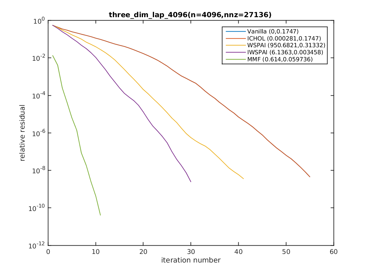
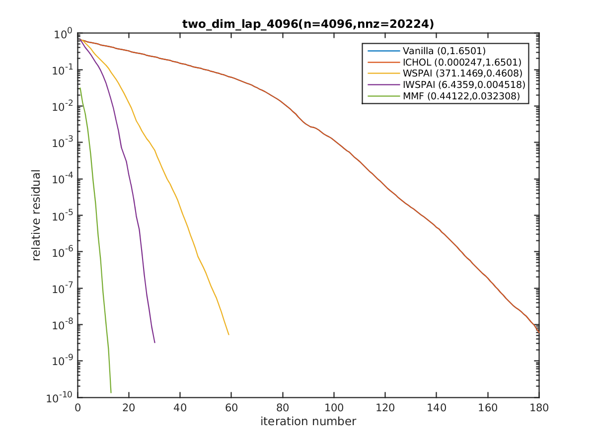
Figure 4: Relative residual as a function of iteration number.

For the off-the-shelf matrices, we only consider the implicit wavelet preconditioner of Hawkins and Chen [16] for comparison. The original wavelet preconditioner of Chan, Tang and Wan [7] is too slow for these large matrices.

Dataset	$n$	no prec.	IWSPAI	MMF prec.
nd3k	8192	455	236	323
nemeth03	9216	4	4	2
net25	9216	460	$\times$	$\times$
fv2	9216	20	20	27
fv3	9216	42	38	52
nemeth12	9216	13	10	3
nemeth11	9216	10	8	3
nemeth09	9216	7	6	3
nemeth14	9216	$\times$	$\times$	8
nemeth04	9216	5	4	3
nemeth23	9216	211	$\times$	$\times$
pf2177	9216	174	$\times$	$\times$
bloweybq	9216	$\times$	8	$\times$
nemeth10	9216	8	7	3
flowmeter0	9216	$\times$	$\times$	9
nemeth25	9216	164	$\times$	$\times$
nemeth24	9216	179	$\times$	$\times$
nemeth15	9216	282	$\times$	70
nopoly	10240	119	108	105
bcsstk17	10240	$\times$	$\times$	266
bundle1	10240	$\times$	$\times$	30
linverse	11264	$\times$	20	$\times$
t2dah	11264	$\times$	$\times$	7
crystm02	13312	1	1	30
Pres_Poisson	14336	436	43	114
bcsstm25	14336	$\times$	$\times$	2
gyro_m	16384	1	1	115
gyro_k	16384	$\times$	$\times$	220
nd6k	16384	$\times$	270	330
bodyy4	16384	184	147	91
t3dl_a	18432	$\times$	141	6
Si5H12	18432	103	71	89
Trefethen_20000b	18432	$\times$	$\times$	8
crystm03	24576	1	1	33
spmsrtls	28672	$\times$	150	$\times$
wathen100	28672	$\times$	$\times$	33
wathen120	32768	$\times$	$\times$	33
mario001	36864	269	$\times$	$\times$
torsion1	36864	41	29	50
bfly	49152	59	$\times$	$\times$
crankseg_2	57344	$\times$	$\times$	246
Ga3As3H12	57344	$\times$	$\times$	104
cant	57344	$\times$	$\times$	83

Figure 5: Iteration counts of GMRES solved to a relative error of $10^{-4}$. $\times$ indicates that the method did not achieve the desired tolerance within 500 iterations.

In Fig. 5 we compare the iteration counts. The best result for each dataset is highlighted in bold. In the majority of datasets, the MMF preconditioner turns out best. However, for a few datasets such as gyro_m, crystm03, crystm02, the implicit wavelet preconditioner outperforms MMF preconditioning.

We remark that the “geometry free” nature of MMF preconditioner makes it more flexible than standard wavelet preconditioners. In particular, MMF can be applied to matrices of any size, not just $p\hskip 1.00006pt2^{s}$. Furthermore, MMF preconditioning is completely invariant to the ordering of the rows/columns, in contrast to, for example, the multiresolution preconditioner of Bridson and Tang [5]. The adaptability of MMF makes it suitable to preconditioning a wide variety of linear systems.

6 Conclusion

We presented a new multiresolution preconditioner for symmetric linear systems that does not depend on any geometric assumptions, and hence can be applied to any coefficient matrix that is assumed to have multiresolution structure, even in the loose sense. Numerical experiments show the effectiveness of the new preconditioner in a range of problems. In our experiments we used default parameters, but with fine tuning our results could possibly be improved further.

It is not yet clear exactly what kind of matrices the new MMF preconditioner is most effective on, in part due to the general nature of the pMMF algorithm. It is possible that specializing MMF to specific types of linear systems would yield even more effective preconditioners.

7 Acknowledgements

We would like to thank Prof. Stuart Hawkins for help with implementing his preconditioner and Prof. Jonathan Weare for discussions. This work was funded by NSF award CCF–1320344.

References

- [1] R. E. Bank, T. F. Dupont, and H. Yserentant, The hierarchical basis multigrid method, Numerische Mathematik, 52 (1988), pp. 427–458.
- [2] M. Benson, Iterative solution of large scale linear systems, Mathematics report, Thesis (M.Sc.)–Lakehead University, 1973.
- [3] M. Benzi, Preconditioning techniques for large linear systems: a survey, Journal of Computational Physics, 182 (2002), pp. 418–477.
- [4] M. Benzi and M. Tuma, A comparative study of sparse approximate inverse preconditioners, Applied Numerical Mathematics, 30 (1999), pp. 305–340.
- [5] R. Bridson and W.-P. Tang, Multiresolution approximate inverse preconditioners, SIAM Journal on Scientific Computing, 23 (2001), pp. 463–479.
- [6] W. L. Briggs, V. E. Henson, and S. F. McCormick, A multigrid tutorial, SIAM, 2000.
- [7] T. F. Chan, W. P. Tang, and W. L. Wan, Wavelet sparse approximate inverse preconditioners, BIT Numerical Mathematics, 37 (1997), pp. 644–660.
- [8] I. Daubechies, Ten lectures on wavelets, SIAM, 1992.
- [9] T. A. Davis and Y. Hu, The University of Florida sparse matrix collection, ACM Transactions on Mathematical Software (TOMS), 38 (2011), p. 1.
- [10] S. Demko, W. F. Moss, and P. W. Smith, Decay rates for inverses of band matrices, Mathematics of Computation, 43 (1984), pp. 491–499.
- [11] I. S. Duff, A. Erisman, C. Gear, and J. K. Reid, Sparsity structure and Gaussian elimination, ACM SIGNUM Newsletter, 23 (1988), pp. 2–8.
- [12] M. Faustmann, J. M. Melenk, and D. Praetorius, -matrix approximability of the inverses of FEM matrices, Numerische Mathematik, 131 (2015), pp. 615–642.
- [13] L. Grasedyck, R. Kriemann, and S. Le Borne, Domain decomposition based LU preconditioning, Numerische Mathematik, 112 (2009), pp. 565–600.
- [14] M. J. Grote and T. Huckle, Parallel preconditioning with sparse approximate inverses, SIAM Journal on Scientific Computing, 18 (1997), pp. 838–853.
- [15] W. Hackbusch, A sparse matrix arithmetic based on -matrices. part I: introduction to -matrices, Computing, 62 (1999), pp. 89–108.
- [16] S. C. Hawkins and K. Chen, An implicit wavelet sparse approximate inverse preconditioner, SIAM Journal on Scientific Computing, 27 (2005), pp. 667–686.
- [17] R. Kondor, N. Teneva, and V. Garg, Multiresolution matrix factorization, in Proceedings of the 31st International Conference on Machine Learning (ICML-14), 2014, pp. 1620–1628.
- [18] R. Kondor, N. Teneva, and P. K. Mudrakarta, Parallel MMF: a multiresolution approach to matrix computation, CoRR, abs/1507.04396 (2015), http://arxiv.org/abs/1507.04396.
- [19] R. Kriemann and S. Le Borne, -FAINV: hierarchically factored approximate inverse preconditioners, Computing and Visualization in Science, 17 (2015), pp. 135–150.
- [20] S. G. Mallat, A theory for multiresolution signal decomposition: the wavelet representation, IEEE Transactions on Pattern Analysis and Machine Intelligence, 11 (1989), pp. 674–693.
- [21] C. C. Paige and M. A. Saunders, Solution of sparse indefinite systems of linear equations, SIAM Journal on Numerical Analysis, 12 (1975), pp. 617–629.
- [22] F. H. Pereira, S. L. L. Verardi, and S. I. Nabeta, A fast algebraic multigrid preconditioned conjugate gradient solver, Applied Mathematics and Computation, 179 (2006), pp. 344–351.
- [23] A. Quarteroni and A. Valli, Numerical approximation of partial differential equations, vol. 23, Springer Science & Business Media, 2008.
- [24] J. W. Ruge and K. Stüben, Algebraic multigrid, Multigrid methods, 3 (1987), pp. 73–130.
- [25] W. Sweldens, The lifting scheme: a construction of second generation wavelets, SIAM Journal on Mathematical Analysis, 29 (1998), pp. 511–546.
- [26] N. Teneva, P. K. Mudrakarta, and R. Kondor, Multiresolution matrix compression, in Artificial Intelligence and Statistics, 2016, pp. 1441–1449.
- [27] M. J. Todd and Y. Ye, A centered projective algorithm for linear programming, Mathematics of Operations Research, 15 (1990), pp. 508–529.
- [28] L. N. Trefethen and D. Bau III, Numerical linear algebra, vol. 50, SIAM, 1997.
- [29] H. A. Van der Vorst, Bi-CGStab: A fast and smoothly converging variant of Bi-CG for the solution of nonsymmetric linear systems, SIAM Journal on Scientific and Statistical Computing, 13 (1992), pp. 631–644.
- [30] C. F. Van Loan, The ubiquitous Kronecker product, Journal of Computational and Applied Mathematics, 123 (2000), pp. 85–100.
- [31] P. S. Vassilevski and J. Wang, Stabilizing the hierarchical basis by approximate wavelets, I: theory, Numerical Linear Algebra with Applications, 4 (1997), pp. 103–126.
- [32] P. S. Vassilevski and J. Wang, Stabilizing the hierarchical basis by approximate wavelets II: implementation and numerical results, SIAM Journal on Scientific Computing, 20 (1998), pp. 490–514.
- [33] Y. Xi, R. Li, and Y. Saad, An algebraic multilevel preconditioner with low-rank corrections for sparse symmetric matrices, SIAM Journal on Matrix Analysis and Applications, 37 (2016), pp. 235–259.
- [34] Y. Ye, Interior-point algorithms for quadratic programming, Recent Developments in Mathematical Programming, (1991), pp. 237–261.
- [35] Y. Ye, On the finite convergence of interior-point algorithms for linear programming, Mathematical Programming, 57 (1992), pp. 325–335.
- [36] H. Yserentant, Hierarchical bases give conjugate gradient type methods a multigrid speed of convergence, Applied Mathematics and Computation, 19 (1986), pp. 347–358.
- [37] H. Yserentant, On the multi-level splitting of finite element spaces, Numerische Mathematik, 49 (1986), pp. 379–412.