labelkeyrgb0,0,1
Option Pricing and Hedging for Discrete Time Autoregressive Hidden Markov Model
Abstract.
In this paper we solve the discrete time mean-variance hedging problem when asset returns follow a multivariate autoregressive hidden Markov model. Time dependent volatility and serial dependence are well established properties of financial time series and our model covers both. To illustrate the relevance of our proposed methodology, we first compare the proposed model with the well-known hidden Markov model via likelihood ratio tests and a novel goodness-of-fit test on the S&P 500 daily returns. Secondly, we present out-of-sample hedging results on S&P 500 vanilla options as well as a trading strategy based on theoretical prices, which we compare to simpler models including the classical Black-Scholes delta-hedging approach.
Key words and phrases:
Option Pricing, Dynamic Hedging, Regime-Switching, Goodness-of-fit, Hidden Markov Models.1. Introduction
The quest for the perfect option pricing model is clearly an important topic in the mathematical finance literature. Cox and Ross, (1976) provided the following observation: if a claim is priced by arbitrage in a world with one asset and one bond, then its value can be found by first adapting the model so that the asset earns the risk-free rate, and then computing the expected value of the claim. The idea of finding a self-financing optimal investment strategy that replicates the terminal payoff of the claim is now known as dynamic hedging.
One can model the underlying asset’s returns with the geometric Brownian motion and retrieve a tractable and intuitive way of pricing and replicating options. This is precisely what Black and Scholes, (1973) proposed. Unfortunately, financial markets are far too complex for a model as simple as this one and this hedging protocol can lead to large hedging errors, as it will be shown later in this paper. The main drawback of this framework is the constant volatility’s assumption. Indeed, volatility seems to vary over time (Schwert,, 1989), (Hamilton and Lin,, 1996), mainly for macroeconomics reason. Furthermore, this model assumes serial independence for the returns, which is also an hypothesis that is violated in general.
Optimal hedging was later introduced, which consists in minimizing the quadratic error of replication. The solutions were derived in continuous time (Schweizer,, 1992) and later in discrete time (Schweizer,, 1995). This methodology can be applied to geometric Brownian motion, or more interestingly to stochastic volatility models.
Hidden Markov models Hamilton, (1989), Hamilton, (1990) were proven to be extremely useful for modeling economic and financial time series. They are robust to time-varying volatility, serial correlation and higher-order moments, which are all well-established stylized facts of asset returns. The premise for these models is that identifiable events can quickly change the characteristics of an asset’s returns. This should be taken into account when pricing a derivative. These events could be on a long horizon - fundamental changes in monetary, fiscal or income policies - or on a shorter horizon - news related to the underlying stock or changes in the target band for the Federal funds rate. However, the classical implementation of an HMM can’t account for multiple horizons.
Elliot’s work on energy finance and interest rate modeling, where mean-reversion is a widely accepted feature, addresses this problem. Wu and Elliott, (2005) introduced a way to parameterize a regime-switching mean-reverting model with jumps. They found the calibration of the model to be difficult because of the small amounts of jumps in the time series exhibited. Elliott et al., (2011) later introduced a similar model with no jumps, and where it is the volatility that is subject to mean-reverting regime-switches. His basis was that volatility, being driven by macroeconomic forces, was not to be modeled by price movements. Hence the need to model it by a hidden Markov chain. Finally, Elliott et al., (2013) investigates the valuation of European and American options under another model where the volatility is subject to regime-switches, but this time the Markov chain being observable. The paper suggest that it would be interesting to develop some methods and their corresponding criteria to determine the optimal number of states for the hidden Markov chain in their setting. This is precisely one of the contributions of our paper.
In light of all the above, we decided to generalize the work of Rémillard et al., (2017): we combine the regime-switching model with an autoregressive parameter to account for trends and mean-reversions (Fama and French,, 1988) without having to change regime. Autoregressive hidden Markov models (ARHMM) have been applied to financial engineering and have shown promising results (Shi and Weigend,, 1997). Still, this model has never been used in conjunction with optimal hedging. We derive the solution of the hedging strategy and obtain derivatives prices under this class of models. It is also noteworthy to add that we will use semi-exact techniques to compute expectations necessary for the optimal hedging, instead of Monte Carlo techniques, which will greatly speed up computations. For parameterization, we will implement the EM algorithm (Dempster et al.,, 1977) to the ARHMM. This method is widely used in unsupervised machine learning in order to find hidden structures, in our case, regimes. In order to choose the optimal number of regimes and to assess the suitability of the model, we propose a new goodness-of-fit test based on the work of Genest et al., (2006) and Rémillard, 2011b . It is based on the Rosenblatt transform and on parametric bootstrap. Compared to Elliot’s work, our model can exhibit mean-reversion, but is not restricted to it. It could thus be more adequate for the modeling of a wider variety of financial assets.
In his famous study Fama, (1965), Fama presented strong and voluminous evidence in favor of the random walk hypothesis. He although suggests that other tests - statistical or profit generating strategies - could either confirm or contradict his findings. In this paper, we will explore both avenues. We will statistically show that the ARHMM is an adequate model for financial modelling using the goodness-of-fit test as well as likelihood ratio tests, and we will show that it is possible to generate money by buying/selling options and replicating them until maturity. To support our approach, we will compare the trading strategy’s returns with different methodologies: Black-Scholes delta-hedging and optimal hedging when assets follow a geometric random walk. We will also compare the hedging results with the delta-hedging using the market’s implicit volatility.
First, we present likelihood ratio test results confirming the ARHMM is a better fit than the classical HMM on S&P daily returns, in particular, because our model has the capacity for mean-reversion. Secondly, empirical pricing and hedging results suggest that our methodology is superior to its counterparts by achieving the best mean-squared error in six out of eight cases, as well as being the most profitable strategy.
The rest of the paper is organized as follows. Section 2 describes the model and implements the EM algorithm for parameter estimation. In addition, we will introduce the goodness-of-fit test and study its suitability in the financial markets. Then, in Section 3, we will state the optimal dynamic discrete time hedging model when assets follow a ARHMM. The results of the implementation of the dynamic hedging strategies will be presented in Section 4. Section 5 concludes.
2. Regime-Switching Autoregressive models
The proposed models are quite intuitive. The regime process is a homogeneous Markov chain on , with transition matrix . At period , if , and the return has value , then at time , with probability , and the return has conditional distribution ; here lower case letters are used to denote a realization of . It follows from this construction that is a Markov process.
For example, for , one could take a Gaussian AR(1) model meaning that given and , , with ; more precisely, the conditional density of at is
| (1) |
where , is a matrix such that as 111This condition ensures that for any , the matrix is well defined and satisfies ., and is a non degenerate covariance matrix. The matrices are mean-reversion parameters. Let be the set of matrices such as and let be the set of symmetric positive definite matrices. Note that is the set of matrices with spectral radius smaller than , meaning that the eigenvalues are all in the unit complex ball of radius ; in particular, is invertible for any . Note that the the so-called Hidden Markov Model is obtained by setting .
2.1. Regime prediction
Since the regimes are not observable, we have to find a way to predict them. This will be of utmost importance for pricing and hedging derivatives.
In many applications, one has to predict an non-observable signal by using observations linked in a certain way to the signal. This is known as a filtering problem (Rémillard,, 2013). In our case, we need to find the most likely regime at time , in other words . It is remarkable that for the present model, one can compute exactly this conditional distribution, given a starting distribution . For more details, see an extension of the Baum-Welch algorithm in Appendix A.
2.1.1. Filtering algorithm
Choose an a priori probability distribution for the regimes. Equivalently, one can choose a positive vector and set , where . The choice of or is not critical since its impact on predictions decays in time and have virtually no impact on terminal regime probabilities for any reasonable time series length. For simplicity, we assume a uniform distribution, i.e. .
For , define , , and . 222The first observation of the sequence is burn-in in order to compute Hence, is the joint density of because
Then if , then for any , and any ,
| (2) | |||||
and
| (3) |
Having computed the conditional probabilities, , one can finally estimate by
| (4) |
i.e. as the most probable regime.
In view of applications, it is preferable to rewrite (3) only in terms of , i.e.,
| (5) |
where
As a result, is the conditional density of given , evaluated at .
2.1.2. Conditional distribution
From the results of the previous section, the joint density of is . Also, for any , the conditional density of given , can be expressed as a mixture, viz.
| (6) |
where
| (7) |
Note that for all , . As a result, it follows that
| (8) |
so the conditional law of given has density
| (9) |
Next, it is easy to check that the conditional law of given has density
2.1.3. Stationary distribution in the Gaussian case
Suppose that the model specified by (1) holds, ergo the innovations are Gaussian. If converges in law to a stationary distribution, for any given starting point , then this distribution must be Gaussian, with mean and covariance matrix . Suppose the Markov chain is ergodic with stationary distribution . Then with probability , , , where is independent of . It then follows that
Similarly, must satisfies , where
| (11) |
with . From the conditions on , there is a norm on the space of matrices such that for every .333Recall that all norms are equivalent. The operator is then a contraction since for any two matrices , , with . Also, since is a covariance matrix whenever is one, and is positive definite, it follows that there is a unique fixed point of , meaning that , and this unique fixed point is a positive definite covariance matrix. If fact, is the limit of any sequence , with a non-negative definite covariance matrix. For example, one could take even take . This provides a way to approximate the limiting covariance by setting for large enough.
2.2. Estimation of parameters
The EM algorithm (Dempster et al.,, 1977) is a quite efficient estimation procedure for incomplete datasets. Under hidden Markov models, observations are partial since is unobservable. The algorithm proceeds iteratively to converge to the maximum likelihood estimation of parameters (Dempster et al.,, 1977). We derived its implementation for ARHMM and the details are in Appendix C. It seems that starting the parameter’s estimation of the ARHMM with the HMM parameters’ estimate (obtained by setting ) was slightly more stable. The optimal number of regimes must be known a priori, an issue we will discuss next.
2.3. Goodness-of-fit test and selection of the number of regimes
To select the optimal number or regimes, one must test the adequacy of fitted models with different number of regimes. This is generally done by using a test based on likelihoods. However, goodness-of-fit tests based on likelihoods are not recommended for regime-switching models (Cappé et al.,, 2005). We opt for a simpler approach based on a parametric bootstrapping. It was shown to work on a large number of dynamic models, including hidden Markov models. The test was built on the work of Genest and Rémillard, (2008) and its implementation is in Appendix D.
2.3.1. Selecting the number of regimes
Choosing the optimal number of regimes. The goodness-of-fit test methodology described in Appendix B produces P-value from Cramér-von Mises type statistics, for a given number of regimes . As suggested in Papageorgiou et al., (2008), it make sense to choose the optimal number of regimes, , as the first for which the P-value is larger than 5%. An illustration of the proposed methodology is given in Section 2.4.
2.4. Application to S&P 500 daily returns
To assess the relevance of our model on real data, we estimated the parameters on the close-to-close log-returns of the daily price series of the S&P 500 Total Return. To find stationary estimation windows, we used a nonparametric changepoint test for a univariate series using a Kolmogorov-Smirnov type statistic (Rémillard,, 2013). We focused on recent data, i.e. from early 2000 to today. We found two stationary estimation window: from 05/01/2004 to 02/01/2008 and from 05/01/2010 to 20/01/2017. We can refer to the former as the 2000’s recovery and 2010’s recovery for the latter. Results of the tests are presented is Table 1. We will also study the interesting period in between, the 2008-2009 Financial Crisis, even though the null hypothesis of stationarity has a -value of .
| Period | -value |
|---|---|
| 2000’s recovery | 39.8 |
| 2008-2009 Financial Crisis | 0.4 |
| 2010’s recovery | 9.7 |
Next, we perform the goodness-of-fit test (GoF for short) described in Appendix D for the ARHMM (AR(1)) as well as for the HMM (AR(0)), as a mean of comparison. The results are presented in Tables 2, 4 and 6. According to the selection methods described in Section 2.3.1, we optimally select a three-regime model for the 2000’s recovery, since is the smallest number of regimes for which the -value is larger than 5%. This is also true for the HMM model. Likewise, we choose a three-regime model for the 2008-2009 Financial Crisis, and a four-regime model for the 2010’s recovery. Note that in the case of the 2010’s Bull markets, a four regime model for the HMM was not enough to get a -value .
Furthermore, to measure the significance of ARHMM over HMM, we perform a likelihood ratio test. This is possible because the HMM is a special case of the ARHMM corresponding to . The corresponding statistic is computed as follow:
where are the model’s parameters estimated under the null hypothesis, i.e. , so the returns follow a Gaussian hidden Markov model, and are the model’s parameters estimated under the alternative, i.e. returns follow an autoregressive hidden Markov model. Under the null hypothesis, this statistic is distributed as a chi-square distribution with the number of degrees of freedom equal to the number of extra parameters in the alternative model. In our case, we have one extra parameter per regime, i.e. , so the number of degrees of freedom is . Hence, under the null hypothesis, . The log-likelihoods of both models, the statistical test and the critical value at a significance level of 5% are also presented in Tables 2, 4 and 6. We clearly reject the null hypothesis for all models, proving we should favor ARHMM over HMM for each dataset.
The estimated parameters for the three periods are presented in Tables 3, 5, and 7, where the mean and standard deviation of each AR(1) and AR(0) Gaussian regime density are respectively denoted by and , and are presented as annualized percentages values. The tables further contains the long-term, i.e. stationary, regime probabilities , together with the estimated transition matrix, .
Regimes are ordered by increasing volatility , and incidentally by decreasing mean , which is in line with what we typically observe on the markets.
| Number of regimes | |||
| 1 | 2 | 3 | |
| GoF -value (ARHMM) | 0 | 0 | 26.51 |
| GoF -value (HMM) | 0 | 0 | 25.12 |
| Log-likelihood (ARHMM) | 3479 | 3542 | 3559 |
| Log-likelihood (HMM) | 3475 | 3539 | 3552 |
| -value (D) | 0.43 | 3.63 | 0.18 |
| AR(0) | AR(1) | |||||
| Parameter | Regime | Regime | ||||
| 1 | 2 | 3 | 1 | 2 | 3 | |
| 31.41 | 13.88 | -17.23 | 34.89 | 6.99 | -21.60 | |
| 2.18 | 10.09 | 18.02 | 3.34 | 11.03 | 18.95 | |
| 0 | 0 | 0 | -0.14 | 0.03 | -0.19 | |
| 0.11 | 0.65 | 0.24 | 0.19 | 0.63 | 0.18 | |
| 0 | 0.92 | 0.08 | 0 | 0.96 | 0.04 | |
| Q | 0.17 | 0.83 | 0 | 0.32 | 0.68 | 0 |
| 0 | 0.03 | 0.97 | 0 | 0.04 | 0.96 | |
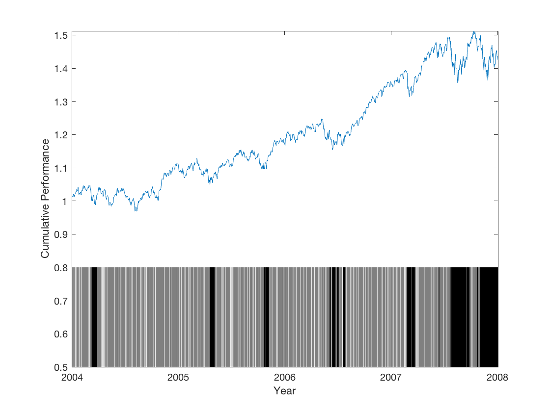
In the case of the 2000’s recovery, Regime 1 is associated to bull markets, which are characterized by strong positive premium and low risk ( and ). It seems that this state is intermittent in the sense that the Markov chain does not stay or has a very small probability of staying in regime 1 since . However, this state is not due to outliers since the percentage of time the Markov chain is in this state is 11% for the HMM and 19% for the ARHMM.
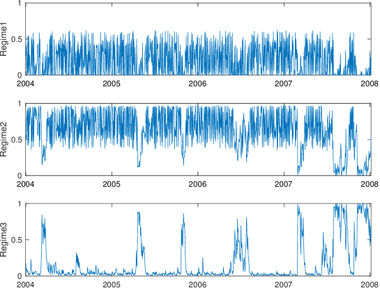
Regime 2 is an intermediate state. Lastly, Regime 3 is associated with bear markets or corrections, as highlighted by the negative premium of -21.60 and the volatility of 18.95. The regimes are less distinct in the HMM case. Also, the likelihood ratio test statistic informs us that ARHMM is a much better fit for this data. Indeed, we observe strong mean-reversion in regime 1 and 3 ( and ). This could explain why the HMM is blurring everything to together. Figure 1 displays the filtered most probable regimes (see Section 2.1 for the filtering procedure) for the whole time series. The regimes are depicted by different shades of grey, ranging from dark for the high volatility regime to white for the low volatility regime. The probability of the regimes, i.e. , are presented in Figure 2. Interestingly enough, the crisis in the subprime mortgage market is adequately captured by the high risk regime.
| Number of regimes | |||
| 1 | 2 | 3 | |
| GoF -value (ARHMM) | 0 | 0 | 59.59 |
| GoF -value (HMM) | 0 | 0 | 72 |
| Log-likelihood (ARHMM) | 1,209 | 1,323 | 1,334 |
| Log-likelihood (HMM) | 1,214 | 1,318 | 1.329 |
| -value (D) | 0.19 | 0.95 | 2.59 |
| AR(0) | AR(1) | |||||
| Parameter | Regime | Regime | ||||
| 1 | 2 | 3 | 1 | 2 | 3 | |
| 74.97 | -5.28 | -66.87 | 72.22 | -0.42 | -64.73 | |
| 5.52 | 23.17 | 57.80 | 5.12 | 22.56 | 55.68 | |
| 0 | 0 | 0 | -0.03 | -0.16 | -0.15 | |
| 0.15 | 0.58 | 0.27 | 0.14 | 0.58 | 0.28 | |
| 0 | 0.97 | 0.03 | 0 | 0.98 | 0.02 | |
| Q | 0.25 | 0.75 | 0 | 0.23 | 0.77 | 0 |
| 0 | 0.01 | 0.99 | 0 | 0.01 | 0.99 | |
The second period studied is pretty interesting. For the 2008-2009 Financial Crisis, regimes are extremely polarized, with expected returns ranging from 72.22 to -64.73. The bear markets regime, i.e. Regime 3, is exceptionally persistent and volatile, as highlighted by and . Once more, we find two regimes exhibiting mean-reversion, i.e. and .
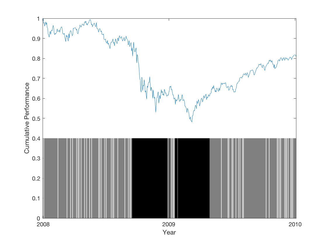
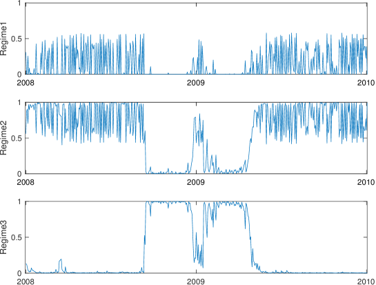
Figure 3 and 4 are analogous to Figure 1 and 2 respectively. We can see that the Markov chain switched to the high risk regime right after the collapse of the investment bank Lehman Brothers. Remarkably, it stayed in that regime throughout almost all the Banking Crisis, even though we observe numerous small upwards trends, meaning many thought we hit the bottom.
| Number of regimes | ||||
| 1 | 2 | 3 | 4 | |
| GoF -value (ARHMM) | 0 | 0 | 0 | 1.56 |
| GoF -value (HMM) | 0 | 0 | 0 | 5.83 |
| Log-likelihood (ARHMM) | 5,696 | 5,936 | 5,985 | 6,012 |
| Log-likelihood (HMM) | 5,694 | 5,931 | 5,981 | 6,006 |
| -value (D) | 4.19 | 1.52 | 4.46 | 3.02 |
| AR(0) | AR(1) | |||||||
| Parameter | Regime | Regime | ||||||
| 1 | 2 | 3 | 4 | 1 | 2 | 3 | 4 | |
| 29.41 | 303.07 | -68.77 | -28.25 | 32.04 | 365.83 | -68.82 | -27.50 | |
| 6.70 | 8.13 | 13.50 | 29.05 | 6.73 | 7.56 | 13.39 | 28.50 | |
| 0 | 0 | 0 | 0 | -0.04 | 0.14 | -0.09 | -0.08 | |
| 0.44 | 0.09 | 0.33 | 0.14 | 0.45 | 0.09 | 0.32 | 0.14 | |
| 0.91 | 0 | 0.09 | 0 | 0.90 | 0 | 0.10 | 0 | |
| Q | 0.47 | 0.07 | 0.45 | 0 | 0.53 | 0.06 | 0.41 | 0 |
| 0 | 0.23 | 0.76 | 0.01 | 0 | 0.23 | 0.76 | 0.01 | |
| 0 | 0.03 | 0 | 0.97 | 0 | 0.03 | 0 | 0.97 | |
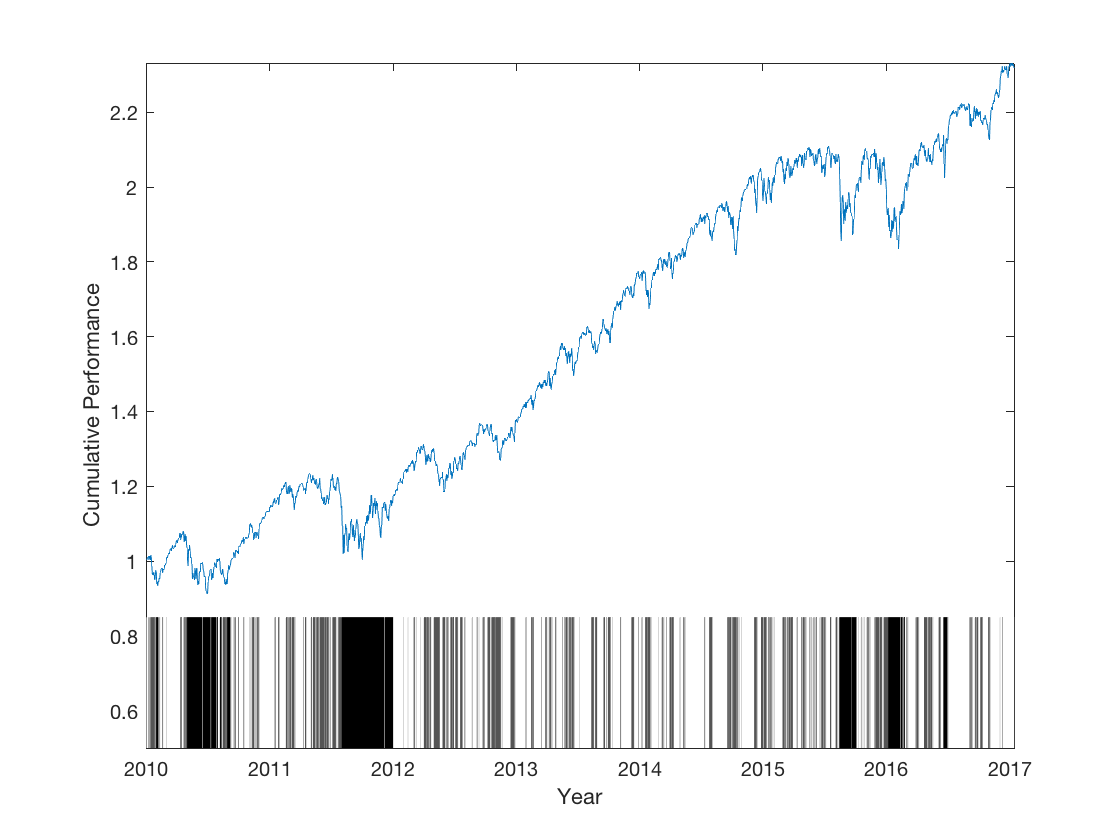
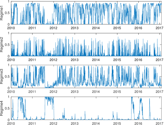
For the last period, we chose four-regimes models. As noted previously, the four-regime HMM did not pass the goodness-of-fit test. We still present the estimated parameters in Table 7, as a mean of comparison. The calibration for this period is less intuitive than the previous ones. The inverse correlation between risk and expected premium is not as strong. Also, both models have a non-persistent regime with huge expected returns, (i.e. regime 2). Nevertheless, we still find modest mean-reversion for two regimes (i.e. regime 3 and 4), and the high-risk regime is highly persistent, as highlighted bu , as it was in the two previous cases. The most probable regimes are displayed in Figure 5, while the probability of the regimes are presented in Figure 6. Interestingly enough, the crisis in the subprime mortgage market is adequately captured by the high risk regime.. The final part of 2011 was marked by fear of the European sovereign debt crisis spreading to Italy and Spain. Once again, the ARHMM isolated the stock markets fall quite accurately.
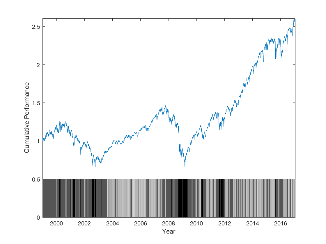
We also estimated the ARHMM on the returns from 01/04/1999 to 01/20/2017. This long period is far from stationary, but it is still interesting to see how the model performs through recessions and recoveries. We chose a four-regime model, as indicated by the goodness-of-fit tests. We can see on Figure 7 that the 2000’s bubble burst and the recent financial meltdown (2008-2009) are both correctly captured by the high risk regimes.
3. Optimal Discrete Time Hedging
In what follows, we use the notations and results from Rémillard and Rubenthaler, (2013).
Denote the price process by , i.e., is the value of underlying assets at period and let a filtration under which is adapted. Further assume is square integrable. Set = , where the discounting factors are deterministic for . We are interested in the optimal initial investment amount and the optimal predictable investment strategy = that minimizes the expected quadratic hedging error for a given payoff, , at time (e.g a call option). Formally, the problem is stated as
| (12) |
where
and is the current value of the replicating portfolio at time . In other words, it is the current value of the optimal predictable investment strategy, ,
for .
To solve (12), set = 1, and define
for
We can now state Theorem 1 of Rémillard and Rubenthaler, (2013), which is a multivariate extension of Schweizer, (1995).
Theorem 1.
Suppose that P-a.s., for 1,…,n. This condition is always respected for regime-switching models. Then, the solution of the minimization problem (12) is , and
| (13) |
where
| (14) |
and and are the present values of and .
Remark 1.
is chosen such that the expected hedging error, G, is zero. Rémillard and Rubenthaler, (2013) also showed that given by
| (15) |
is the optimal investment at period t so that the value of the portfolio at period is as close as possible to in term of mean square error , in particular, .
can be interpreted as the option price at period . By increasing the number of hedging periods, should tend to a price under a risk-neutral measure; see, e.g., Rémillard and Rubenthaler, (2016). For example, when there is only one regime, the density is Gaussian and fixed at 0, tends to the usual Black-Scholes price. The detailed optimal hedging implementation for ARHMM is described in Appendix E. It then follows that
| (16) |
| (17) |
To derive the optimal hedging algorithm, we also need the following result, valid for a general ARHMM.
First, write , where is the vector with components , and is the diagonal matrix with diagonal elements , .
The proof of the following theorem is given in Appendix E.1.
Theorem 2.
For any , , , , and , with , where , , and are deterministic functions given respectively by
| (18) | |||||
| (19) | |||||
with , and . If in addition , then , where
| (21) |
and
| (22) |
where
| (23) |
For example, for a call option with strike , .
3.1. Implementation issues
There are two main problems related to the implementation of the hedging strategy: , , , and defined in expressions (18)-(23) must be approximated and regimes must be predicted.
We discretize , functions of the underlying values with a grid . In a similar manner, we discretize and functions of the underlying values and . To solve the recursion given by (21)-(23), Rémillard et al., (2017) interpolate and extrapolate linearly the simulated outcomes on , using a stratified Monte Carlo sampling procedure. Because the simulations are computationally expensive and introduce variability, we propose a novel technique to approximate these integrals using semi-exact calculations, inspired by Rémillard, (2013) Chapter 3. The details for the semi-exact calculations are presented in Appendix E.3.
We also included the Monte Carlo sampling procedure as a mean of comparison. Interestingly, we found that by simply rescaling the Monte Carlo samples to the desired mean and volatility, we achieved results as accurate as the semi-exact calculations, as pointed out in Section 3.3.
As for defining the points on the grid, previous literature suggest choosing equidistant points marginally covering at least 3 standard deviations
under the respective highest volatility regimes. Importantly, we found that strategically choosing the points with respect to the percentiles of simulated processes significantly reduces the number of points needed while keeping the accuracy at a reasonable level.
Next, we need to predict based on and and so on. The predicted regime is is the one having the largest probability given the information on prices up to time , i.e. the given by (4). Note that this methodology introduces a bias. We also studied the less biased approach of weighting the regimes proportionally to , but since the results were comparable and did not lead to any significant improvement, they are omitted from the analysis. For more details on regime predictions, see section 2.1.
| (24) |
is approximated by while the remaining monies, , are invested in the riskless asset. Next, as is observed, one firsts computes the actual portfolio value , then predicts the current regime and finally approximates the optimal weights . This process is iterated until expiration of the option.
3.1.1. Using regime predictions
Here, we obtain option prices and strategies that depend on the unobservable regimes , since is a Markov chain. However, François et al., (2014) proposed a very interesting approach: they showed that is Markov, so one can obtain prices and hedging strategies depending on instead. This makes sense financially. However, this new Markov chain lives in a -dimensional space, because the values of belong to the simplex . François et al., (2014) considered only 2 regimes and one asset, so the real dimension is . When , this becomes numerically intractable.
3.2. Global hedging
In practice, an expected hedging error characterized by will emerge. In other words, the replicating portfolio at period t will not be worth the optimal investment . Under the Black-Scholes setting, such error is unaccounted for since derivatives can be replicated perfectly (in continuous time). In contrast, under the proposed optimal hedging protocol, the exposures depend on the replicating portfolio, (see equation 13), which in turn depends on the past strategy path.
Under extreme scenarios, the replication of a call option might lead to optimal exposures greater than one share. Intuitively, this feature is optimal with respect to closing the gap between and .
3.3. Simulated hedging errors
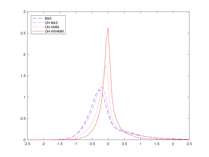
To assess the proposed strategy’s accuracy, we simulated 10000 trajectories under ARHMM and hedge identical options under different hedging strategies. To be realistic, the parameters were taken from Table 3. The hedging methodologies are the classical Black-Scholes delta-hedging (B&S) and optimal hedging under ARHMM (OH-ARHMM), HMM (OH-HMM) and Gaussian (OH-B&S) returns (i.e., considering only regime). We also compared semi-exact approximation to Monte-Carlo. The option in question is a call with and equal to 100, risk-free rate , 3 month maturity (63 days) with daily hedging. The main hedging error statistics are given in Table 8, while the estimated densities are displayed in Figure 8.
OH-ARHMM achieves a 33% reduction in RMSE compared to B&S and OH-B&S and a 26% to OH-HMM. The latter is quite impressive, as it highlights how big of an impact the autoregressive dynamic has.
| B&S | OH-B&S | HMM | HMM MC | ARHMM | ARHMM MC | |
|---|---|---|---|---|---|---|
| Average | -0.105 | -0.084 | 0.004 | 0.003 | 0.025 | 0.030 |
| Median | -0.236 | -0.202 | -0.085 | -0.086 | -0.019 | -0.019 |
| Volatility | 0.611 | 0.626 | 0.559 | 0.559 | 0.411 | 0.412 |
| Skewness | 1.715 | 1.948 | 1.639 | 1.629 | 4.644 | 4.738 |
| Kurtosis | 7.737 | 9.558 | 9.464 | 9.356 | 71.834 | 78.219 |
| Minimum | -1.658 | -1.658 | -4.649 | -4.633 | -2.477 | -2.413 |
| VaR (1%) | -1.110 | -1.118 | -1.087 | -1.086 | -0.749 | -0.741 |
| VaR (99%) | 2.069 | 2.227 | 1.987 | 1.982 | 1.526 | 1.531 |
| Maximum | 4.886 | 6.725 | 6.538 | 6.520 | 12.958 | 14.266 |
| RMSE | 0.620 | 0.632 | 0.559 | 0.559 | 0.411 | 0.413 |
4. Out-of-sample vanilla pricing and hedging
4.1. Methodology
To exhibit the proposed hedging protocol, we buy and sell vanilla options on the S&P 500 depending on the how the market prices compare with our theoretical prices. Then, we hedge the positions until expiration. We then assess the impact of model specification on the delta-hedging strategy by examining the statistical properties of the hedging error and of the strategy’s returns. All hedging portfolios are re-balanced on a daily basis, as is often assumed in the volatility timing literature; see e.g., Fleming et al., (2001).
The market price of an option is defined as the last (i.e. as 4:15 PM EST) midpoint between the bid and the ask. The price of the underlying is its listed close value. For simplicity, we neglect issues related to time-varying discount rates by assuming constant continually compounded daily rates. Risk-free rates, , are linearly interpolated for a given maturity, , from the zero-coupon U.S. yield curve.
Remark 2.
For the implementation, we chose to present only the results using the most probable regime for the computation of the hedging strategy. These results are a little bit better than those obtained by weighting the hedging strategy according to the probability of occurrence of the regimes at period .
4.1.1. The underlying
We make the reasonable assumption the spot S&P 500 is investable and tradable at a minimal cost. The forward rate is retrieved for the maturities of interest directly from the option data at hand, as proposed by Buraschi and Jackwerth, (2001). From put-call parity, the option implied forward value at , , is
where and are respectively the call and put values expiring at with strike and is the at-the-money strike value minimizing for all strikes offered by the exchange. We use at-the-money options because they are the most liquid and are thus less likely to provide cash-and-carry type arbitrage opportunities. We then compute the daily forward rate as and the associated daily discounting factor , which reflects the current risk-free return on capital net of the implied continuous dividend yield.
4.1.2. Option dataset
Exchange-traded options on the S&P 500 are European, heavily traded and have a high number of strikes and maturities.
To assess the accuracy of our model, we will analyze two periods with very different characteristics: the 2008 Financial Crisis, and a chunk of the recent recovery. Dates range from 09/24/2007 to 09/20/2009 and from 09/23/2013 to 07/08/2015, respectively. This will help us discern the impact on hedging and pricing when a dramatic regime change occurs, in the former, and when it does not, in the latter.
In order to minimize the effect of varying maturities, we will build the dataset of options having a maturity of about year, more precisely from 231 to 273 trading days till expiration. Also, because in-the-money and out-of-the-money are less liquid, we will only include options where moneyness (strike value divided by the underlying value), is between 0.9 and 1.1. This leaves us with a total of 180 options for the first period, and 478 for the second.
Note that at a given date, more than one option can meet these criteria.
4.1.3. Backtesting
We apply the AR(1) regime-switching optimal hedging methodology with 3 regimes (ARHMM). We chose 3 regimes because it is the number of regimes that seemed the best given the time windows studied, which we will describe in the next paragraph. We will compare it to the case with 1 regime and fixed at 0, corresponding to the optimal hedging under the Black-Scholes model (OH-B&S).
For each option in the dataset, we estimate the ARHMM parameters on the S&P 500 log-returns with a 500 and 2000 day trailing window. We choose to backtest using 2 estimation windows in order to have a more in depth understanding of model specification on pricing and hedging. The 2000 day trailing window will always include the previous financial meltdown, i.e., dot-com bubble for our first analysis, and the 2008 financial crisis for the second one. The 500 day trailing window won’t. Similarly, we applied this methodology to all the hedging protocols included in the analysis, which will be introduced below.
From Merton, (1973), for a given moneyness, the value of an option is homogeneous of degree one with respect to the underlying value. Thus, for each inception date, we normalize the option prices, the strike values and the underlying path at an initial S&P 500 value of 100. Results can thus be aggregated through time and interpreted as a percentage of S&P 500. Note that for each inception date, the hedging protocols are applied out-of-sample until maturity.
To ensure comparability, OH-B&S assumes the stationary distribution of the ARHMM when the autoregressive parameter . The OH-B&S optimal hedging exposure is derived from an algorithm similar to the one presented in Section 3. Optimal hedging under unconditional distributions is presented in Rémillard, (2013). Both strategies minimize the expected quadratic hedging error under their respective null hypothesis, namely that the returns follow an autoregressive regime-switching model (ARHMM), and a Gaussian model (OH-B&S).
OH-B&S methodology is not to be confused with the classical Black-Scholes delta hedging protocol. Indeed, the terminology only reflects the fact that we hedge and price under the Black-Scholes framework hypothesis, namely that assets follow geometric Brownian motions. Even though the OH-B&S prices converge to the usual Black-Scholes prices as the number of hedging periods tends to infinity, the discrete time hedging strategies will not necessarily be the same. For this reason, the classical Black-Scholes delta-hedging methodology (B&S) is also considered. Similarly to OH-B&S, the B&S volatility is calibrated to the stationary volatility of ARHMM.
We will add a final benchmark to our analysis, one that reflects how well the market would have hedged the same options, namely the delta-hedging methodology where the volatility is calibrated to the implied volatility at each hedging period (B&S-M). It will inform us how well the models compare to market’s intuition.
The effect of using the implied volatility was discussed in Carr, (2002). However, his theoretical analysis cannot be performed here.
To recap, we will buy and sell options depending on their market value compared to the theoretical prices, and hedge the positions until maturity. We will analyse the P&L of the different methodologies, as well as the hedging errors. Two periods will be studied: the 2008 Financial Crisis and a chunk of the following recovery spanning from mid-2013 to mid-2015.
4.2. Empirical results
We define the hedging error as the present value of the liability minus the present value of terminal portfolio . The options’ maturity being set to one year, the annualized root-mean-squared hedging error can be computed by . This realized risk is the empirical counterpart of the quantity we minimized and as such, is the most relevant metric for comparing the different models. Keep in mind that there is a lot of overlap in our dataset, so the hedging error values are not independent, nor identically distributed since the moneyness or other parameters are not constant. Despite these inconveniences, the hedging errors are still useful to compare the models.
Concerning the trading strategy, if the market is overvalued with respect to the model, we sell the option and hedge our position. Thus, the present value of the return is . If the market is undervalued, we buy the option and hedge our position. The return will be the negative of the former.
4.2.1. 2008-2009 financial crisis
In this section, we will focus on options with inception dates from September 2007 to September 2009. This period is really interesting. In the first part, the market experienced a huge increase in volatility and decrease in returns. In the second, the opposite.
We will first turn our attention to the 500 trailing estimation window case. Table 9 and Figure 9 present the hedging error’s statistics and density approximation. Figure 10 presents the results of the trading strategy, i.e., the cumulative value of a portfolio that traded the 90 options. The x axis is the cumulative number of options traded in chronological order. In this case, ARHMM is by far the superior methodology. It achieved the best hedging error considering all the metrics for both calls and puts. Further, it was the best trading strategy for both type of options, even though the hedging errors are almost entirely negative in the calls case. Note that the statistic “Bias” refers to the difference between the market price and the theoretical price. Therefore, it is always for the BS-M, since the implied volatility is used.
When volatility increases and returns turn negative, the puts’ value increase and one needs to be hedge accordingly. B&S and B&S-M failed to do so, resulting in huge hedging errors and great losses portfolio wise.
| Calls | Puts | |||||||
|---|---|---|---|---|---|---|---|---|
| B&S-M | B&S | OH-B&S | ARHMM | B&S-M | B&S | OH-B&S | ARHMM | |
| RMSE | 3.87 | 5.27 | 4.53 | 0.61 | 39.95 | 42.52 | 4.53 | 0.98 |
| Bias | 0 | -4.52 | -4.37 | -5.35 | 0 | -1.05 | -0.91 | -1.87 |
| VaR 1% | -7.64 | -12.02 | -12.47 | -3.17 | -28.39 | -33.24 | -12.47 | -3.18 |
| Median | 2.9 | 3.82 | 2.68 | -1.65e-04 | 30.78 | 29.77 | 2.68 | 0.01 |
| VaR 99% | 9.16 | 8.61 | 7.57 | -1.97e-09 | 72.9 | 77.22 | 7.57 | 4.75 |
(a) 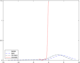 (b)
(b) 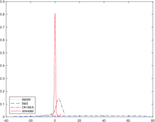
(a) 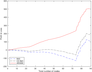 (b)
(b) 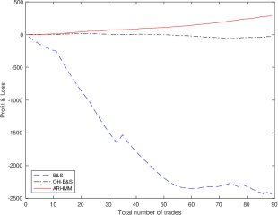
Similar results are presented in Table 10 and Figures 11 and 12, although the trailing estimation window, previously set to 500 days, is now 2000 days. This estimation window includes another financial crisis, the Dot-com Bubble. The same conclusion as the previous experience can be drawn.
| Calls | Puts | |||||||
|---|---|---|---|---|---|---|---|---|
| B&S-M | B&S | OH-B&S | ARHMM | B&S-M | B&S | OH-B&S | ARHMM | |
| RMSE | 3.87 | 4.26 | 3.15 | 0.33 | 39.95 | 40.87 | 3.15 | 1.25 |
| Bias | 0 | -4.86 | -4.69 | -4.91 | 0 | -1.4 | -1.23 | -1.44 |
| VaR 1% | -7.64 | -4.76 | -4.27 | -1.43 | -28.39 | -28.68 | -4.27 | -1.4 |
| Median | 2.9 | 3.26 | 1.93 | 0.01 | 30.78 | 27.74 | 1.93 | 0.35 |
| VaR 99% | 9.16 | 8.93 | 7.62 | 0.33 | 72.9 | 74.76 | 7.62 | 4.83 |
(a) 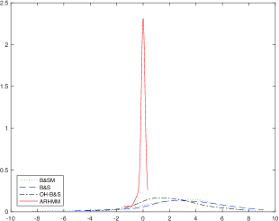 (b)
(b) 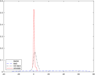
(a) 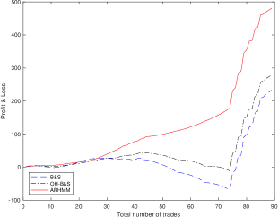 (b)
(b) 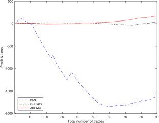
4.2.2. 2013-2015 Bull markets
Our second and last analysis focuses on a part of the recent recovery spanning from September 2013 to August 2015. This period is quite the opposite of a financial crash. It is characterized by steady returns and low volatility.
Again, we start with the small trailing estimation window. We present the results for calls and puts in Table 11 and Figures 13 and 14. Considering the hedging errors, OH-B&S and ARHMM achieved the best and pretty similar statistics for both put and calls. Similarly to the previous experience in Section 4.2.1, B&S and B&S-M replicated poorly the put options.
| Calls | Puts | |||||||
|---|---|---|---|---|---|---|---|---|
| B&S-M | B&S | OH-B&S | ARHMM | B&S-M | B&S | OH-B&S | ARHMM | |
| RMSE | 1.09 | 1.64 | 0.84 | 0.99 | 18.12 | 11.6 | 0.84 | 0.99 |
| Bias | 0 | 0.12 | 0.22 | 0.59 | 0 | -4.08 | -3.98 | -3.62 |
| VaR 1% | -2.63 | -2.53 | -1.45 | -2.47 | -41.63 | -26.59 | -1.45 | -2.46 |
| Median | -0.2 | 0.14 | -0.02 | -0.01 | -12.12 | -8.6 | -0.02 | -0.01 |
| VaR 99% | 1.39 | 4.42 | 3.7 | 3.54 | 9.42 | 6.78 | 3.7 | 3.53 |
(a) 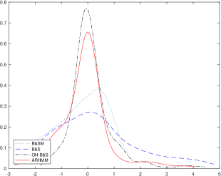 (b)
(b) 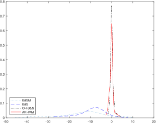
(a) 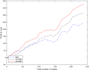 (b)
(b) 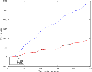
Finally, the results for the longer estimation window case is presented in Table 12 and Figures 15 and 16. This is probably the worst environment for the ARHMM, as the estimation window includes a financial crisis (i.e. 2008-2009 Financial Crisis) and the out-of-sample returns are slow and steady. Because our trading strategy takes into account the actual hedging error, according to (13), the simpler models should perform better. In spite of that, ARHMM managed to perform better than B&S and B&-M for the hedging errors of the puts.
The fact that pricing bias for the calls are strongly positive is noteworthy. In theory, the pricing bias should be negative, to account for the risk premium. In this case, it seems that the market was pretty confident about returns and volatility staying low. In insight, it was right.
| Calls | Puts | |||||||
|---|---|---|---|---|---|---|---|---|
| B&S-M | B&S | OH-B&S | ARHMM | B&S-M | B&S | OH-B&S | ARHMM | |
| RMSE | 1.09 | 5.32 | 4.84 | 8.57 | 18.12 | 14.75 | 4.84 | 8.6 |
| Bias | 0 | 4.71 | 4.54 | 4.18 | 0 | 0.52 | 0.34 | -0.01 |
| VaR 1% | -2.63 | -10 | -8.93 | -31.27 | -41.63 | -27.66 | -8.93 | -31.39 |
| Median | -0.2 | -4.67 | -4.09 | -2.82 | -12.12 | -12.5 | -4.09 | -2.81 |
| VaR 99% | 1.39 | -1.79 | -1.76 | -0.04 | 9.42 | 1.41 | -1.76 | -0.04 |
(a) 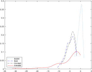 (b)
(b) 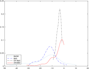
(a) 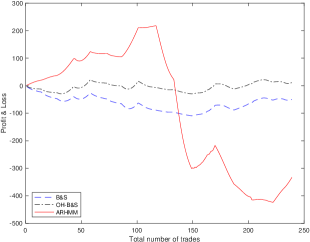 (b)
(b) 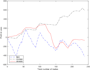
Lastly, we aggregated the P&L over all the experiences for B&S, OH-B&S and ARHMM in Table 13. For a fair comparison, we normalized the number of traded options in each cases to 100. Remember that the option prices, strike prices and underlying path are also normalized at an initial S&P 500 value of 100. Impressively, ARHMM accomplished a 106% increase in P&L compared to the second best, OH-B&S, for the 2-year trailing window, and is only 9% behind the first for the 8-year case, which is again OH-B&S.
| Trailing window (years) | B&S | OH-B&S | ARHMM |
|---|---|---|---|
| 2 | -1286.78 | 685.32 | 1409.54 |
| 8 | -1761.77 | 594.56 | 546.38 |
Overall, by achieving the best Root Mean Square Error (RMSE) two times out of four for both the 2-year and 8-year window, and by being the most profitable strategy three times out of four for the 2-year window and two times out of four for the 8-year window, the ARHMM is the superior hedging protocol.
However, the practitioners should keep in mind that if the ARHMM is estimated on a window including a financial crisis, they should expect higher hedging errors than the simpler models if returns stay slow and steady. From our results, we strongly suggest to use a 2-year trailing window as it consistently achieved an RMSE lower than 1, i.e., the ARHMM can accurately hedge options in a financial crisis without ever seeing one.
5. Conclusion
In this paper, we propose an autoregressive hidden Markov model to fit financial data, and we show how to implement an optimal hedging strategy when the underlying asset returns follow an autoregressive regime-switching random walk.
First, we present estimation and filtering procedures for the ARHMM. In order to determine the optimal number of regimes, we propose a novel goodness-of-fit test for univariate and multivariate ARHMM based on the work of Bai, (2003), Genest and Rémillard, (2008) and Rémillard et al., (2017).
To illustrate the proposed strategy, we model three daily return series of the S&P 500. Using likelihood test, we show that the ARHMM is a much better fit than the classical HMM, particularly because it has the capacity to model mean-reversion.
Moreover, we present the implementation of the discrete-time optimal hedging algorithm minimizing the mean-squared hedging error. Because it further performs pricing, we implemented a trading strategy consisting of selling overpriced and buying underpriced options and hedging the position till maturity. Out of eight cases and compared to three other hedging protocols, our strategy achieves the best root-mean-squared hedging error four times and is the most profitable strategy five times. Furthermore, it realized the best total P&L.
Because of its ability to model regime switches as well as mean-reversion, it would be interesting to see this model applied to multivariate time series. The hedging algorithm can also be applied to multivariate or American options.
References
- Bai, (2003) Bai, J. (2003). Testing parametric conditional distributions of dynamic models. The Review of Economics and Statistics, 85(3):531–549.
- Black and Scholes, (1973) Black, F. and Scholes, M. (1973). The pricing of options and corporate liabilities. Journal of Political Economy, 81:637–654.
- Buraschi and Jackwerth, (2001) Buraschi, A. and Jackwerth, J. (2001). The price of a smile: hedging and spanning in option markets. The Review of Financial Studies, 14(2):495–527.
- Cappé et al., (2005) Cappé, O., Moulines, E., and Rydén, T. (2005). Inference in Hidden Markov Models. Springer Series in Statistics. Springer, New York.
- Carr, (2002) Carr, P. (2002). FAQ’s in option pricing theory. Technical report, NYU.
- Cox and Ross, (1976) Cox, J. and Ross, S. (1976). The valuation of options for alternative stochastic processes. Journal of Financial Economics, 3:145 –166.
- Dempster et al., (1977) Dempster, A. P., Laird, N. M., and Rubin, D. B. (1977). Maximum likelihood from incomplete data via the EM algorithm. J. Roy. Statist. Soc. Ser. B, 39:1–38.
- Diebold et al., (1998) Diebold, F. X., Gunther, T. A., and Tay, A. S. (1998). Evaluating density forecasts with applications to financial risk management. International Economic Review, 39(4):863–883.
- Elliott et al., (2013) Elliott, R. J., Chan, L., and Siu, T. K. (2013). Option valuation under a regime-switching constant elasticity of variance process. Appl. Math. Comput., 219(9):4434–4443.
- Elliott et al., (2011) Elliott, R. J., Miao, H., and Wu, Z. (2011). An asset pricing model with mean reversion and regime switching stochastic volatility. In The Oxford handbook of nonlinear filtering, pages 960–989. Oxford Univ. Press, Oxford.
- Fama, (1965) Fama, E. F. (1965). The behavior of stock-market prices. Journal of Business, 38(1):34– 105.
- Fama and French, (1988) Fama, E. F. and French, K. R. (1988). Dividend yields and expected stock returns. Journal of Financial Economics, pages 3–25.
- Fleming et al., (2001) Fleming, J., Kirby, C., and Ostdiek, B. (2001). The economic value of volatility timing. The Journal of Finance, 56(1):329–352.
- François et al., (2014) François, P., Gauthier, G., and Godin, F. (2014). Optimal hedging when the underlying asset follows a regime-switching Markov process. European Journal of Operational Research, 237(1):312–322.
- Genest et al., (2006) Genest, C., Quessy, J.-F., and Rémillard, B. (2006). Goodness-of-fit procedures for copula models based on the integral probability transformation. Scand. J. Statist., 33:337–366.
- Genest and Rémillard, (2008) Genest, C. and Rémillard, B. (2008). Validity of the parametric bootstrap for goodness-of-fit testing in semiparametric models. Ann. Inst. H. Poincaré Sect. B, 44:1096–1127.
- Hamilton, (1989) Hamilton, J. D. (1989). A new approach to the economic analysis of nonstationary time series and the business cyle. Eonometrica, pages 357–384.
- Hamilton, (1990) Hamilton, J. D. (1990). Analysis of time series subject to changes in regime. J. Econometrics, 45(1-2):39–70.
- Hamilton and Lin, (1996) Hamilton, J. D. and Lin, G. (1996). Stock market volatility and business cycle. Journal of Applied Econometrics, pages 573–593.
- Merton, (1973) Merton, R. C. (1973). Theory of rational option pricing. The Bell Journal of Economics and Management Science, 4(1):141–183.
- Papageorgiou et al., (2008) Papageorgiou, N., Rémillard, B., and Hocquard, A. (2008). Replicating the properties of hedge fund returns. Journal of Alternative Invesments, 11:8–38.
- (22) Rémillard, B. (2011a). Tests of independence. In Lovric, M., editor, International Encyclopedia of Statistical Science, pages 1598–1601. Springer Berlin Heidelberg.
- (23) Rémillard, B. (2011b). Validity of the parametric bootstrap for goodness-of-fit testing in dynamic models. Technical report, SSRN Working Paper Series No. 1966476.
- Rémillard, (2013) Rémillard, B. (2013). Statistical Methods for Financial Engineering. Chapman and Hall/CRC Financial Mathematics Series. Taylor & Francis.
- Rémillard et al., (2017) Rémillard, B., Hocquard, A., Lamarre, H., and Papageorgiou, N. A. (2017). Option pricing and hedging for discrete time regime-switching model. Modern Economy.
- Rémillard and Rubenthaler, (2013) Rémillard, B. and Rubenthaler, S. (2013). Optimal hedging in discrete time. Quantitative Finance, 13(6):819–825.
- Rémillard and Rubenthaler, (2016) Rémillard, B. and Rubenthaler, S. (2016). Option pricing and hedging for regime-switchin geometric Brownian motion models. Working paper series, SSRN Working Paper Series No. 2599064.
- Schweizer, (1992) Schweizer, M. (1992). Mean-variance hedging for general claims. Ann. Appl. Probab., 2(1):171–179.
- Schweizer, (1995) Schweizer, M. (1995). Variance-optimal hedging in discrete time. Math. Oper. Res., 20(1):1–32.
- Schwert, (1989) Schwert, G. W. (1989). Why does stock market volatility change over time? Journal of Finance, 44:1115– 1153.
- Shi and Weigend, (1997) Shi, S. and Weigend, A. S. (1997). Taking time seriously: hidden Markov experts applied to financial engineering. Computational Intelligence for Financial Engineering (CIFEr), pages 244–252.
- Wu and Elliott, (2005) Wu, P. and Elliott, R. J. (2005). Parameter estimation for a regime-switching mean-reverting model with jumps. Int. J. Theor. Appl. Finance, 8(6):791–806.
Appendix A Extension of Baum-Welch Algorithm
For and , define
Also, for and , define
and let be the conditional density of , given and . Further set . Note that , for any .
The proof of the following proposition is given in Appendix B.
Proposition 1.
For all ,
| (25) | |||||
| (26) | |||||
| (27) | |||||
| (28) |
In particular,
| (29) |
Appendix B Proof of Proposition 1
Let and be given. Set , and . Let denotes the density of . If follows from the definition of conditional expectations that for any bounded measurable functions , , and ,
As a by-product, one gets
Since the last equation holds for any and , it follows that (25) holds true.
Next, let be the density of . Then
As a by-product,
proving (27). It is easy to extend the last argument to the case .
Finally,
As a by-product, the latter can also be written as
proving (28). It is easy to extend the last argument to the case . This completes the proof. ∎
Appendix C Estimation of regime-switching models
To describe the EM algorithm for the estimation, suppose that at step , one has the parameters , , , , .
Let , and set and , , where and are given in Proposition 1.
Then, at step , for , one has
| (30) | |||||
| (31) | |||||
| (33) |
where , .
The proof is given in the next section.
C.1. Proof of the EM algorithm for the estimation
The EM algorithm for estimating parameters consists of two steps, expectation and maximization:
E-Step: Compute the conditional probabilities.
for all and .
M-Step:
Let be the set of transition matrices with positive entries. Suppose that , and . Then the log-likelihood is
It then follows that
If are the parameters at step , then the parameters at step are
C.1.1. Estimation for Gaussian AR(1) regime-switching models (M-Step)
For the estimation procedure, we assume the densities are given by (1), so .
In this case, the function to minimize is given by
Let . It then follows that for any ,
| (34) |
| (35) |
and
| (36) |
where , , since
where , and for any non singular matrix ,
The latter is true because for any .
Appendix D Goodness-of-fit Test for Autoregressive Hidden Markov Model
In this Appendix, we state the goodness-of-fit test, which can be performed to asses the suitability of a Gaussian AR(1) regime-switching models as well as to select the optimal number of regimes, . The proposed test, based on the work of Diebold et al., (1998), Genest and Rémillard, (2008) and Rémillard, 2011a , uses the Rosenblatt’s transform. For conciseness, we detail the implementation for two dimensional Gaussian AR(1) regime-switching models, but the approach can be easily generalized.
D.1. Conditional distribution functions and the Rosenblatt’s transform.
Let be fixed an be a random vector with density . For any , denote by the density of , and by the density of given . Further denote by the distribution function associated with density . By convention, denotes the density of . Then, the Rosenblatt’s transform
is such that is uniformly distributed in .
For example, if is the density of a bivariate Gaussian distribution with mean and covariance matrix
is the density of a Gaussian distribution with mean and variance , with . These results can easily be extended to the Gaussian AR(1) distribution.
However, for regime-switching random walks models, past returns must also be included in the conditioning information set. For any , the (-dimensional) Rosenblatt’s transform corresponding to the density (6) conditional on is given by
and
for .
Suppose is a size n sample of -dimensional vectors drawn from a joint (continuous) distribution . Also, let be the parametric family of Gaussian AR(1) regime-switching models with regimes. Formally, the hypothesis to be tested is
Under the null, it follows that are independent and uniformly distributed over , where are the Rosenblatt’s transforms conditional on the set of parameters .
Since is unknown, it must be estimated by some . Then, the -, are uniformly distributed over and independent. We next propose a test statistic based on these pseudo observations.
D.2. Test statistic
The test statistic builds from the following empirical process:
To test against we propose a Cramér-von Mises type statistic:
Since is almost uniformly distributed on under the null hypothesis, large values of should lead to rejection of the null hypothesis. Unfortunately, the limiting distribution of the test statistic will depend on the unknown parameter set, . Since it is impossible to construct tables, we use a different methodology, namely parametric bootstrap, to compute -values. The validity of the parametric bootstrap approach has been shown for a wide range of assumptions in Genest and Rémillard, (2008). These results were recently extended to dynamic models (Rémillard, 2011b, ), including regime-switching random walks. In this paper, we generalized the procedure to AR(1) Gaussian regime-switching model by conditioning the Rosenblatt’s transform on the previous return.
D.3. Parametric bootstrap algorithm
-
a)
For a given number of regimes, estimate parameters with computed from the EM algorithm applied to
-
b)
Compute the test statistic,
from the estimated pseudo observations, , for .
-
c)
For some large integer N (say 1000), repeat the following steps for every :
-
i)
Generate a random sample from distribution
-
ii)
Compute by applying the EM algorithm to the simulated sample, .
-
iii)
Let for , and finally compute
-
i)
Then, the approximate -value for the test based on the Cramér von Mises statistic is given by
Appendix E Optimal Hedging
E.1. Proof of Theorem 2
Proof.
First, we show this is true for the off-line random sequences and . The result is clearly true for . Now,
since is a Markov process. For the same reason,
As a result, , so
Therefore, . The rest of the proof is done by induction. Assume this is true for , then we have to prove this is true for . Now
since is a Markov process. Similarly,
Hence, , so
Therefore,
Suppose now that . Using induction together with (16), one gets
E.2. Optimal hedging algorithm
Since these variables are weighted expectations they can be approximated by using Monte Carlo simulations, coupled with interpolations. This method was proposed in Papageorgiou et al., (2008). Because the simulations are computationally expensive and introduce variance, we propose a novel technique to approximate these expectations using semi-exact calculations, based on Rémillard, (2013).
E.3. Semi-exact calculations.
By defining a grid, i.e. , one can approximate a function by the continuous piecewise linear function
| (38) |
where
| (39) | |||
| (40) |
where
Remember that . The formula for is shown later.
Now, let be the cumulative distribution function of the standard normal distribution and let be the associated density. Also, . If , and if are given, then for any , one has
and
where for any ,
In particular,
This way, we can approximate , and as follows.
For any and any , set
and
where .
To approximate and , we need to define a second grid, defined by . can be also be approximated by a product of continuous piecewise linear functions viz.
where
using the results in Appendix E.4.
As a result, for and for ,
with the convention that the integral is if
There is a similar expression for , namely
Note that = and = for all . For example, for all , while for a put option with strike , , for all .
E.4. Bi-linear interpolation
One wants to interpolate by over . Set , .
Then , where
E.5. Simulation of Gaussian ARHMM(1)
If , then with with probability and then , where and .
Also, when , a random sample of size from is given by , with . So the sequence of innovations are independent of .
In this case, every integral is approximated by
In particular, this means that for any ,