A Robust t-process Regression Model with Independent Errors

Abstract

Gaussian process regression (GPR) model is well-known to be susceptible to outliers. Robust process regression models based on t-process or other heavy-tailed processes have been developed to address the problem. However, due to the nature of the current definition for heavy-tailed processes, the unknown process regression function and the random errors are always defined jointly and thus dependently. This definition, mainly owing to the dependence assumption involved, is not justified in many practical problems and thus limits the application of those robust approaches. It also results in a limitation of the theory of robust analysis. In this paper, we propose a new robust process regression model enabling independent random errors. An efficient estimation procedure is developed. Statistical properties, such as unbiasness and information consistency, are provided. Numerical studies show that the proposed method is robust against outliers and has a better performance in prediction compared with the existing models. We illustrate that the estimated random-effects are useful in detecting outlying curves.

1 Introduction

In regression analysis, we are interested in modelling the relationship between response $y$ and covariate $\mbox{\boldmath${x}$}\in\mathcal{X}\subset R^{p}$. A nonparametric regression usually uses $E(y|\mbox{\boldmath${x}$})$ to fit $y$, based on the model $y=E(y|\mbox{\boldmath${x}$})+e,$ where $e$ is an error term. Let $f_{0}(\mbox{\boldmath${x}$})=E(y|\mbox{\boldmath${x}$})$ be a fixed unknown function of ${x}$. Then, the nonparametric regression model is rewritten as

$${}y=f_{0}(\mbox{\boldmath${x}$})+e.$$ (1)

To estimate function $f_{0}$, this paper considers a process regression model

$$y(\mbox{\boldmath${x}$})=f(\mbox{\boldmath${x}$})+\epsilon(\mbox{\boldmath${x}$}),$$ (2)

where $f(\mbox{\boldmath${x}$})$ is a random function and $\epsilon(\mbox{\boldmath${x}$})$ is an error process. In model (2), $f$ can be treated as a nonparametric random effect and thus this model can be called a nonparametric random effect functional regression model.

When $f$ and $\epsilon$ are independent Gaussian processes (GPs), the model (2) is called Gaussian process regression (GPR) model. The details about the GPR model can be found in Rasmussen and Williams (2006), Shi and Choi (2011). Recent developments include GPR analysis for batch data (Shi et al., 2007), GPR for single-index model (Gramacy and Lian, 2012) and generalized GPR for non-Gaussian functional data (Wang and Shi, 2014). However, it is well-known that the GPR model is susceptible to outliers. To overcome this problem, robust methods are developed based on t-process and other heavy tailed processes; for example, Shah et al. (2014) used a simple t-process to replace a GP; Wang et al. (2017) proposed an extended t-process regression model (eTPR); and Cao et al. (2017) developed robust models based on other heavy-tailed processes such as Slash process and contaminated-normal process. Heavy-tailed processes, particularly t-process, have been used frequently in many different areas to build a robust model, for example, Yu et al. (2007) and Zhang and Yeung (2010) used t-process to build a multi-task learning model, and Xu et al. (2011) employed matrix-variate t-process and a variational approximation method to construct a sparse matrix-variate block model. However, in these robust process regression models, the unknown regression function $f$ is defined jointly with random errors $\epsilon$, and thus they are dependent. Although this brings technical convenience in implementation, the dependence assumption may not be justified in many practical problems and is also not necessary in developing a theory.

In model (2), the regression function $f$ is the main part, describing the regression relationship between the response variable $y$ and the covariates ${x}$. The estimation of unknown $f$ converges to the true function $f_{0}(\mbox{\boldmath${x}$})=E(y|\mbox{\boldmath${x}$})$ when a GPR model is assumed as the sample size tends to infinity (see e.g. Choi and Schervish, 2007; Seeger et al., 2008; Shi and Choi, 2011). The error $\epsilon(\mbox{\boldmath${x}$})$ is usually not dependent on the covariates, otherwise the dependent part can be merged with $f(\mbox{\boldmath${x}$})$. Purely because of technical convenience, $f$ and $\epsilon$ are defined jointly when heavy-tailed processes are used for robust approaches. In this paper, we propose a new approach in which $f$ and $\epsilon$ are separately modeled using extended t-processes (ETPs), not jointly. Hereafter, we name this new robust model as independent error model while the existing models as joint error models.

When $f\sim GP$ and $\epsilon\sim GP$, the joint error model is the same as the independent error model (GPR model) because the sum of two GPs is again a GP. However, in general, the independent error model behaves differently from the joint error model. The former is more flexible and suited to practical application as we shall show. We will also show that the independent error model with TP errors is more robust than the corresponding joint error models, and the function estimator is less sensitive to outlying curves.

The independent error models however involve intractable integrations in the calculation of predictive mean and variance. To address the problem, an efficient estimation procedure is developed via h-likelihood (see e.g. Lee et al., 2006). We also extend the idea to build a process regression model for batched functional data. Statistical properties, such as unbiasness and information consistency, will be shown. Simulation studies show that the proposed method is robust against outlying curves, and application to real data demonstrates that the proposed method provides stable results no matter whether data consist of observations from subject with odd responses. In the research, we also have an interesting finding: the values of estimated random effects can be used to detect outlying curves.

The remainder of the paper is organized as follows. Section 2 presents an independent error regression model and studies predictive distribution of function $f$. In section 3, a general functional regression model for batch data is studied and an h-likelihood estimation procedure is proposed to calculate the prediction. Numerical studies and real examples, including detection of outlying curves, are given in Section 4. All the proofs are presented in Appendix.

2 Independent error regression models

To study a robust independent error regression model, we introduce an extended t-process (ETP) as follows. For a random function $f(\cdot):\mathcal{X}\rightarrow R$, if

$$f|r\sim GP(h,rk)~{}~{}{\mbox{and}}~{}~{}r\sim IG(\nu,\nu-1),$$

then $f$ follows an ETP, denoted by $f\sim ETP(\nu,h,k)$, where $h(\cdot):\mathcal{X}\rightarrow R$ is a mean function, $k(\cdot,\cdot):\mathcal{X}\times\mathcal{X}\rightarrow R$ is a covariance kernel, $GP(h,k)$ stands for a Gaussian process with mean function $h$ and covariance kernel $k$, and $IG(\nu,\nu-1)$ is an inverse gamma distribution with parameter $\nu$ and the density function of

$$g_{\nu}(r)=\frac{1}{\Gamma(\nu)}(\frac{\nu-1}{r})^{\nu+1}\frac{1}{\nu-1}\exp{(-\frac{\nu-1}{r})},$$

having $E(r)=1$ and $Var(r)=1/(\nu-2)$. Here, $r$ is a random effect, affecting the covariance kernel of the GP.

In functional regression, it is convenient to set $h=0$. Thus, we set

$$GP(0,k)=GP(k)\text{ and }ETP(\nu,0,k)=ETP(\nu,k)$$

if no confusion occurs. Note that $GP(k)=ETP(\infty,k)$ with a constant $r=1.$ In model (2), suppose that $f$ and $\epsilon$ are independent random processes, for example,

• GP-GP model: $f\sim GP(k)$ and $\epsilon\sim GP(k_{\epsilon})$;

• GP-TP model: $f\sim GP(k)$ and $\epsilon\sim ETP(\nu_{1},k_{\epsilon})$;

• TP-TP model: $f\sim ETP(\nu_{0},k)$ and $\epsilon\sim ETP(\nu_{1},k_{\epsilon})$;

• TP-GP model: $f\sim ETP(\nu_{0},k)$ and $\epsilon\sim GP(k_{\epsilon})$,

where $k$ is a covariance kernel for the process $f$ and $k_{\epsilon}$ is that for the process $\epsilon$. We usually set $k_{\epsilon}(\mbox{\boldmath${u}$},\mbox{\boldmath${v}$})=\phi I(\mbox{\boldmath${u}$}=\mbox{\boldmath${v}$})$ for ${u}$, $\mbox{\boldmath${v}$}\in\mathcal{X}$. Here $I(\cdot)$ is an indicator function.

Let ${\mathcal{D}}=\{(y_{k},\mbox{{\boldmath${x}$}${}_{k}$}),k=1,...,n\}$ be the observed data set from model (1), where $y_{k}=y(\mbox{{\boldmath${x}$}${}_{k}$})$. The GP-GP model is the well-known GPR model with an explicit conditional prediction process of $f|{\mathcal{D}}$. Note that in the GPR model $f+\epsilon\sim GP(k+k_{\epsilon})$. However, the conditional prediction process of $f|{\mathcal{D}}$ does not have close forms for the rest of models, and it actually involves intractable integrations. We will propose an efficient implementation method via h-likelihood and will use the TP-TP model as an example to illustrate the idea.

2.1 Predictive distributions

Based on the construction of ETP, suppose that $f$ and $\epsilon$ are generated by,

$$f|r_{0}\sim GP(r_{0}k),~{}~{}r_{0}\sim\mathrm{IG}(\nu_{0},\nu_{0}-1),$$

$$\epsilon|r_{1}\sim GP(r_{1}k_{\epsilon}),~{}~{}r_{1}\sim\mathrm{IG}(\nu_{1},\nu_{1}-1),$$

$$r_{0}\text{ and }r_{1}\text{ are independent.}$$

When $r_{0}=r_{1}$, we have

$$f+\epsilon|r_{0}\sim\mathrm{GP}(r_{0}k+r_{0}k_{\epsilon}),\text{ }r_{0}\sim\mathrm{IG}(\nu_{0},\nu_{0}-1).$$

Then, the resulting process for $f+\epsilon$ is the eTPR, a joint error model. Thus, conditional on $r_{0}$, the sum of the eTPRs becomes an eTPR again. This setting is convenient for implementation and makes the derivation of the theory easy, but has a drawback as we shall show.

In the TP-TP model,

$$y(\cdot)|f,r_{1}\sim GP\left(f,~{}r_{1}k_{\epsilon}\right),$$

$$y(\cdot)|r_{0},r_{1}\sim GP\left(0,~{}r_{0}k+r_{1}k_{\epsilon}\right)=GP\left(r_{0}k+r_{1}k_{\epsilon}\right),$$

$$r_{0}\sim\mathrm{IG}(\nu_{0},\nu_{0}-1),~{}r_{1}\sim\mathrm{IG}(\nu_{1},\nu_{1}-1),$$

where $y(\cdot)$ is the response function. Parameters $\nu_{0}$ and $\nu_{1}$ are pre-specified here, but they can be estimated in the model for batch data as we shall show.

When ${\mbox{\boldmath${r}$}}=(r_{0},r_{1})^{T}$ is given, $y$ and $f$ have a GPR model. Thus, the results for the GPR model can be extended to the above model given ${r}$. For the observed data ${\mathcal{D}}$, we have

$$\mbox{{\boldmath${f}$}}(\mbox{{\boldmath${X}$}})|r_{0},\mbox{{\boldmath${X}$}}\sim N(0,~{}r_{0}\mbox{{\boldmath${K}$}${}_{n}$}),$$ (3)

$$\mbox{{\boldmath${y}$}}|\mbox{{\boldmath${f}$}},\mbox{{\boldmath${r}$}},\mbox{{\boldmath${X}$}}\sim N\left(\mbox{{\boldmath${f}$}${}_{n}$},~{}\phi r_{1}\mbox{{\boldmath${I}$}${}_{n}$}\right),$$ (4)

$$\mbox{{\boldmath${y}$}}|\mbox{{\boldmath${r}$}},\mbox{{\boldmath${X}$}}\sim N(0,~{}\mbox{{\boldmath${C}$}${}_{r}$}),$$ (5)

where $\mbox{\boldmath${X}$}=(\mbox{{\boldmath${x}$}${}_{1}^{T}$},...,\mbox{{\boldmath${x}$}${}_{n}^{T}$})^{T}$, $\mbox{\boldmath${y}$}=(y_{1},...,y_{n})^{T}$, $\mbox{{\boldmath${f}$}${}_{n}$}=\mbox{{\boldmath${f}$}}(\mbox{{\boldmath${X}$}})=(f(\mbox{{\boldmath${x}$}${}_{1}$}),...,f(\mbox{{\boldmath${x}$}${}_{n}$}))^{T}$, $\mbox{{\boldmath${K}$}${}_{n}$}=(k_{kl})_{n\times n}$ with $k_{kl}=k(\mbox{{\boldmath${x}$}${}_{k}$},\mbox{{\boldmath${x}$}${}_{l}$})$, and $\mbox{{\boldmath${C}$}${}_{r}$}=r_{0}\mbox{{\boldmath${K}$}${}_{n}$}+\phi r_{1}\mbox{{\boldmath${I}$}${}_{n}$}$. From (3)-(5), we have

$$f(\mbox{{\boldmath${X}$}})|\mbox{\boldmath${r}$},{\mathcal{D}}\sim N(\mbox{{\boldmath${\mu}$}${}_{r}$},\mbox{{\boldmath${\Sigma}$}${}_{r}$})$$

with

$$\mbox{{\boldmath${\mu}$}${}_{r}$}=E(f(\mbox{{\boldmath${X}$}})|\mbox{\boldmath${r}$},{\mathcal{D}})=r_{0}\mbox{{\boldmath${K}$}${}_{n}$}\mbox{{\boldmath${C}$}${}_{r}^{-1}$}\mbox{{\boldmath${y}$}},$$ (6)

$$\mbox{{\boldmath${\Sigma}$}${}_{r}$}=Var(f(\mbox{{\boldmath${X}$}})|\mbox{\boldmath${r}$},{\mathcal{D}})=r_{0}\mbox{{\boldmath${K}$}${}_{n}$}-r_{0}^{2}\mbox{{\boldmath${K}$}${}_{n}$}\mbox{{\boldmath${C}$}${}_{r}^{-1}$}\mbox{{\boldmath${K}$}${}_{n}$}.$$ (7)

For a new data point ${z}$, let $\mbox{{\boldmath${k}$}${}_{z}$}=(k(\mbox{\boldmath${z}$},\mbox{{\boldmath${x}$}${}_{1}$}),...,k(\mbox{\boldmath${z}$},\mbox{{\boldmath${x}$}${}_{n}$}))^{T}$. Similar to (6) and (7) it is easy to show

$$f(\mbox{{\boldmath${z}$}})|\mbox{\boldmath${r}$},{\mathcal{D}}\sim N(\mbox{{\boldmath${\mu}$}${}_{r}^{*}$},\mbox{{\boldmath${\Sigma}$}${}_{r}^{*}$})$$

with

$$\mbox{{\boldmath${\mu}$}${}_{r}^{*}$}=E(f(\mbox{{\boldmath${z}$}})|\mbox{\boldmath${r}$},{\mathcal{D}})=r_{0}\mbox{{\boldmath${k}$}${}_{z}^{T}$}\mbox{{\boldmath${C}$}${}_{r}^{-1}$}\mbox{{\boldmath${y}$}},$$

$$\mbox{{\boldmath${\Sigma}$}${}_{r}^{*}$}=Var(f(\mbox{{\boldmath${z}$}})|\mbox{\boldmath${r}$},{\mathcal{D}})=r_{0}k(\mbox{\boldmath${z}$},\mbox{\boldmath${z}$})-r_{0}^{2}\mbox{{\boldmath${k}$}${}_{z}^{T}$}\mbox{{\boldmath${C}$}${}_{r}^{-1}$}\mbox{{\boldmath${k}$}${}_{z}$}.$$

Remark 1 Let $\mbox{{\boldmath${C}$}}=\mbox{{\boldmath${K}$}${}_{n}$}+\phi\mbox{{\boldmath${I}$}${}_{n}$}$. When $r_{0}=r_{1}=r$, the model becomes an eTPR joint error model in Wang et al. (2017). From (6) we have

$$E(f(\mbox{{\boldmath${X}$}})|\mbox{\boldmath${r}$},\mathcal{D})=\mbox{{\boldmath${K}$}${}_{n}$}\mbox{{\boldmath${C}$}${}^{-1}$}\mbox{{\boldmath${y}$}},$$

which does not depend on random effect ${r}$ and is exactly the conditional mean of $f(\mbox{{\boldmath${X}$}})|\mathcal{D}$ from a GPR model. From (6) and (7) we have

$$Var(f(\mbox{{\boldmath${X}$}})|\mathcal{D})= E\{Var(f(\mbox{{\boldmath${X}$}})|\mbox{\boldmath${r}$},\mathcal{D})|\mathcal{D}\}$$

$$= s_{0}\left(\mbox{{\boldmath${K}$}${}_{n}$}-\mbox{{\boldmath${K}$}${}_{n}$}\mbox{{\boldmath${C}$}${}^{-1}$}\mbox{{\boldmath${K}$}${}_{n}$}\right),$$

where

$$s_{0}=E(r|\mathcal{D})=\frac{2(\nu_{0}-1)+\mbox{{\boldmath${y}$}${}^{T}$}\mbox{{\boldmath${C}$}${}^{-1}$}\mbox{{\boldmath${y}$}}}{2(\nu_{0}-1)+n}.$$

$s_{0}$ stands for the difference in predictive variance between the GPR model and the eTPR joint error model. As $n\rightarrow\infty$, $s_{0}\rightarrow 1$, consequently the eTPR joint error model tends to the GPR. Thus, the robustness of the joint error model is deteriorated when $n$ is large. By contrast, in the independent error models with $r_{0}\neq r_{1}$, both mean and variance are different from those in the joint models; see (6) and (7), where mean and variance depend on $r_{0}$ and $r_{1}$. This makes the independent error model to be robust even when $n$ is large, resulting in a better performance than the joint error models in the presence of outliers.

3 General independent error models for batch data

More generally, model (1) can be extended to a functional regression model for batch functional data,

$$y_{ijk}=f_{0i}(\mbox{\boldmath${x}$}_{ijk})+\epsilon_{ijk},~{}~{}i=1,...,I,j=1,...,J,k=1,...n,$$ (8)

where $y_{ijk}$ is the $k$th observed data under the $j$th curve in the $i$the group, $f_{0i}(\mbox{\boldmath${x}$}_{ijk})$ is the value of unknown function $f_{0i}(\cdot)$ at the $p\times 1$ observed covariate $\mbox{{\boldmath${x}$}${}_{ijk}$}\in\mathcal{X}\subset R^{p}$ and $\epsilon_{ijk}$ is an error term. In the old (young) dataset which is discussed in Section 4, there are $I=2$ groups, $J=12$ or 13 subjects and $n=180$ observed times.

To estimate true unknown functions $f_{0i}$, we consider a process regression model

$$y_{ij}(\mbox{\boldmath${x}$})=f_{i}(\mbox{\boldmath${x}$})+\epsilon_{ij}(\mbox{\boldmath${x}$}),~{}~{}i=1,...,I,j=1,...,J,$$ (9)

where $f_{i}(\mbox{\boldmath${x}$})$ is a random function, $\epsilon_{ij}(\mbox{\boldmath${x}$})$ is an error process for $\mbox{\boldmath${x}$}\in\mathcal{X}$, $y_{ijk}=y_{ij}(\mbox{{\boldmath${x}$}${}_{ijk}$})$ and $\epsilon_{ijk}=\epsilon_{ij}(\mbox{{\boldmath${x}$}${}_{ijk}$})$. In the TP-TP model, we assume $f_{i}$ and $\epsilon_{ij}$ are independent and

$$f_{i}\sim ETP(\nu_{0},k_{i}){\mbox{~{}and~{}}}\epsilon_{ij}\sim ETP(\nu_{1},k_{\epsilon i}),~{}~{}i=1,...,I$$

where $k_{i}$ is a covariance kernel and $k_{\epsilon i}(\mbox{\boldmath${u}$},\mbox{\boldmath${v}$})=\phi_{i}I(\mbox{\boldmath${u}$}=\mbox{\boldmath${v}$})$ for ${u}$, $\mbox{\boldmath${v}$}\in\mathcal{X}$. Under this setup with $J=1$, Wang et al. (2017) discussed a joint error eTPR model. Similar to the discussion in Section 2, $f_{i}$ and $\epsilon_{ij}$ can be defined by,

$$f_{i}|r_{i0}\sim GP(r_{i0}k_{i}),~{}~{}r_{i0}\sim\mathrm{IG}(\nu_{0},\nu_{0}-1),$$

$$\epsilon_{ij}|r_{ij}\sim GP(r_{ij}k_{\epsilon i}),~{}~{}r_{ij}\sim\mathrm{IG}(\nu_{1},\nu_{1}-1),$$

$$r_{i0},r_{i1},...,r_{iJ}\text{ are independent,}~{}~{}i=1,...,I.$$

When $I=J=1$, parameters $\nu_{0}$ and $\nu_{1}$ are not estimable, because there are only two random effects $r_{10}$ and $r_{11}$ such that $r_{10}$ and $r_{11}$ are confounded with the covariance kernels $k_{1}$ and $k_{\epsilon 1}$. Following Wang et al. (2017), when $I=J=1$, a convenient way is to set $\nu_{0}=\nu_{1}=1.05$. When $I>1$, $\nu_{0}$ and $\nu_{1}$ are estimable.

Without loss of generality, we set $\mbox{{\boldmath${x}$}${}_{i1k}$}=...=\mbox{{\boldmath${x}$}${}_{iJk}$}=\mbox{{\boldmath${x}$}${}_{ik}$}$ $(i=1,...,I,k=1,...,n)$, which means the same observed covariates $\{\mbox{{\boldmath${x}$}${}_{i1}$},...,\mbox{{\boldmath${x}$}${}_{in}$}\}$ for $J$ different curves in the $i$th group. Let ${\mbox{\boldmath${X}$}}_{i}=(\mbox{{\boldmath${x}$}${}_{i1}$},...,\mbox{{\boldmath${x}$}${}_{in}$})^{T}$, $\mbox{{\boldmath${y}$}${}_{ij}$}=(y_{ij}(\mbox{{\boldmath${x}$}${}_{i1}$}),...,y_{ij}(\mbox{{\boldmath${x}$}${}_{in}$}))^{T}$, ${\mbox{\boldmath${y}$}_{i}}=(\mbox{{\boldmath${y}$}${}_{i1}^{T}$},...,\mbox{{\boldmath${y}$}${}_{iJ}^{T}$})^{T}$ and ${\mathcal{D}}_{n}=\{\mbox{{\boldmath${X}$}${}_{i}$},\mbox{{\boldmath${y}$}${}_{i}$},i=1,...,I\}$.

3.1 Predictive distributions

For model (9), we have

$$\mbox{{\boldmath${Y}$}${}_{i}$}|f_{i},\mbox{{\boldmath${r}$}${}_{i}$}\sim GP\left(\mbox{{\boldmath${b}$}${}_{J}$}\bigotimes f_{i},~{}\mbox{{\boldmath${r}$}${}_{ei}$}\bigotimes k_{\epsilon i}\right),$$

$$\mbox{{\boldmath${Y}$}${}_{i}$}|\mbox{{\boldmath${r}$}${}_{i}$}\sim GP\left(0,~{}r_{i0}\mbox{\boldmath${A}$}\bigotimes k_{i}+\mbox{{\boldmath${r}$}${}_{ei}$}\bigotimes k_{\epsilon i}\right)=GP\left(r_{i0}\mbox{\boldmath${A}$}\bigotimes k_{i}+\mbox{{\boldmath${r}$}${}_{ei}$}\bigotimes k_{\epsilon i}\right),$$

$$r_{i0}\sim\mathrm{IG}(\nu_{0},\nu_{0}-1),~{}r_{ij}\sim\mathrm{IG}(\nu_{1},\nu_{1}-1),~{}j=1,...,J,$$

where $\mbox{{\boldmath${Y}$}${}_{i}$}=(y_{i1}(\cdot),...,y_{iJ}(\cdot))^{T}$, $\mbox{{\boldmath${r}$}${}_{i}$}=(r_{i0},r_{i1},...,r_{iJ})^{T}$, ${r}$_ei is a $J\times J$ diagonal matrix with diagonal components $\{r_{i1},...,r_{iJ}\}$, $\mbox{{\boldmath${b}$}${}_{J}$}=(1,...,1)^{T}$ is a $J$-length vector of 1’s, ${A}$ is a $J\times J$ matrix with all elements of 1, and $\bigotimes$ stands for Kronecker product. Denote that ${\mbox{\boldmath${r}$}}=(\mbox{{\boldmath${r}$}${}_{1}^{T}$},...,\mbox{{\boldmath${r}$}${}_{I}^{T}$})^{T}$. Based on the observed data ${\mathcal{D}}_{n}$, we can show that

$$\mbox{{\boldmath${f}$}${}_{in}$}=\mbox{{\boldmath${f}$}${}_{i}$}(\mbox{{\boldmath${X}$}${}_{i}$})|r_{i0},\mbox{{\boldmath${X}$}${}_{i}$}\sim N(0,~{}r_{i0}\mbox{{\boldmath${K}$}${}_{in}$}),$$

$$\mbox{{\boldmath${y}$}${}_{i}$}|\mbox{{\boldmath${f}$}${}_{i}$},\mbox{{\boldmath${r}$}${}_{i}$},\mbox{{\boldmath${X}$}${}_{i}$}\sim N\left(\mbox{{\boldmath${b}$}${}_{J}$}\bigotimes\mbox{{\boldmath${f}$}${}_{in}$},~{}\phi_{i}\mbox{{\boldmath${r}$}${}_{ei}$}\bigotimes\mbox{{\boldmath${I}$}${}_{n}$}\right),$$

$$\mbox{{\boldmath${y}$}${}_{i}$}|\mbox{{\boldmath${r}$}${}_{i}$},\mbox{{\boldmath${X}$}${}_{i}$}\sim N(0,~{}\mbox{{\boldmath${C}$}${}_{ri}$}),$$

where $\mbox{{\boldmath${f}$}${}_{i}$}(\mbox{{\boldmath${X}$}${}_{i}$})=(f_{i}(\mbox{{\boldmath${x}$}${}_{i1}$}),...,f_{i}(\mbox{{\boldmath${x}$}${}_{in}$}))^{T}$, $\mbox{{\boldmath${K}$}${}_{in}$}=(k_{ijl})_{n\times n}$ with $k_{ijl}=k_{i}(\mbox{{\boldmath${x}$}${}_{ij}$},\mbox{{\boldmath${x}$}${}_{il}$})$, and $\mbox{{\boldmath${C}$}${}_{ri}$}=r_{i0}\mbox{\boldmath${A}$}\bigotimes\mbox{{\boldmath${K}$}${}_{in}$}+\phi_{i}\mbox{{\boldmath${r}$}${}_{ei}$}\bigotimes\mbox{{\boldmath${I}$}${}_{n}$}$.

Again, it gives

$$f_{i}(\mbox{{\boldmath${X}$}${}_{i}$})|\mbox{\boldmath${r}$},{\mathcal{D}}_{n}\sim N(\mbox{{\boldmath${\mu}$}${}_{ri}$},\mbox{{\boldmath${\Sigma}$}${}_{ri}$})$$

with

$$\mbox{{\boldmath${\mu}$}${}_{ri}$}=E(f_{i}(\mbox{{\boldmath${X}$}${}_{i}$})|\mbox{\boldmath${r}$},{\mathcal{D}_{n}})=r_{i0}(\mbox{{\boldmath${b}$}${}_{J}^{T}$}\bigotimes\mbox{{\boldmath${K}$}${}_{in}$})\mbox{{\boldmath${C}$}${}_{ri}^{-1}$}\mbox{{\boldmath${y}$}${}_{i}$},$$ (10)

$$\mbox{{\boldmath${\Sigma}$}${}_{ri}$}=Var(f_{i}(\mbox{{\boldmath${X}$}${}_{i}$})|\mbox{\boldmath${r}$},{\mathcal{D}_{n}})=r_{i0}\mbox{{\boldmath${K}$}${}_{in}$}-r_{i0}^{2}(\mbox{{\boldmath${b}$}${}_{J}^{T}$}\bigotimes\mbox{{\boldmath${K}$}${}_{in}$})\mbox{{\boldmath${C}$}${}_{ri}^{-1}$}(\mbox{{\boldmath${b}$}${}_{J}$}\bigotimes\mbox{{\boldmath${K}$}${}_{in}$}).$$ (11)

Remark 2 Under a special case of $r_{i0}=r_{i1}=...=r_{iJ}=r$ which is actually a joint error model, ${\mu}$_ri in (10) is independent of ${r}$, thus it becomes the conditional mean of $f_{i}(\mbox{{\boldmath${X}$}${}_{i}$})|\mathcal{D}_{n}$, the same mean as the one from a GPR model. Equation (11) shows that

$$Var(f_{i}(\mbox{{\boldmath${X}$}${}_{i}$})|\mathcal{D}_{n})=s_{0i}\left(\mbox{{\boldmath${K}$}${}_{in}$}-(\mbox{{\boldmath${b}$}${}_{J}^{T}$}\bigotimes\mbox{{\boldmath${K}$}${}_{in}$})\mbox{{\boldmath${C}$}${}_{i}^{-1}$}(\mbox{{\boldmath${b}$}${}_{m}$}\bigotimes\mbox{{\boldmath${K}$}${}_{in}$})\right),$$

where $\mbox{{\boldmath${C}$}${}_{i}$}=\mbox{{\boldmath${K}$}${}_{in}$}+\phi_{i}\mbox{{\boldmath${I}$}${}_{n}$}$, and

$$s_{0i}=E(r|\mathcal{D}_{n})=\frac{2(\nu_{0}-1)+\mbox{{\boldmath${y}$}${}_{i}^{T}$}\mbox{{\boldmath${C}$}${}_{i}^{-1}$}\mbox{{\boldmath${y}$}${}_{i}$}}{2(\nu_{0}-1)+nJ}.$$

This special case with $J=1$ is the eTPR model discussed in Wang et al. (2017).

3.2 Estimation procedure

In independent error models, $E(f_{i}(\mbox{\boldmath${X}$})|\mbox{\boldmath${r}$},\mathcal{D}_{n})$ and $Var(f_{i}(\mbox{\boldmath${X}$})|\mbox{\boldmath${r}$},\mathcal{D}_{n})$ depend on unknown random effect ${r}$. One method to calculate them is to integrate out ${r}$ via conditional distribution of $\mbox{\boldmath${r}$}|{\mathcal{D}_{n}}$, that is

$$E(f_{i}(\mbox{\boldmath${X}$})|{\mathcal{D}_{n}})=\int E(f_{i}(\mbox{\boldmath${X}$})|\mbox{\boldmath${r}$},{\mathcal{D}_{n}})g(\mbox{\boldmath${r}$}|{\mathcal{D}_{n}})d\mbox{\boldmath${r}$}$$

$$Var(f_{i}(\mbox{\boldmath${X}$})|{\mathcal{D}_{n}})=\int\left(Var(f_{i}(\mbox{\boldmath${X}$})|\mbox{\boldmath${r}$},{\mathcal{D}_{n}})+(E(f_{i}(\mbox{\boldmath${X}$})|\mbox{\boldmath${r}$},{\mathcal{D}_{n}}))^{2}\right)g(\mbox{\boldmath${r}$}|{\mathcal{D}_{n}})d\mbox{\boldmath${r}$}$$

$$\hskip 85.35826pt-(E(f_{i}(\mbox{\boldmath${X}$})|{\mathcal{D}_{n}}))^{2},$$

where $g(\mbox{\boldmath${r}$}|{\mathcal{D}_{n}})$ is the conditional density function of $\mbox{\boldmath${r}$}|{\mathcal{D}_{n}}$. Due to the complicated form of $g(\mbox{\boldmath${r}$}|{\mathcal{D}_{n}})$, integrations involved in the above equations are intractable. An alternative way is to use MCMC, but it is computationally too demanding. In this paper, an h-likelihood method is proposed to overcome this problem.

To implement the h-likelihood method, it is necessary to estimate the unknown covariance kernel $k_{i}(\cdot,\cdot)$. We choose a covariance kernel from a function family such as a squared exponential kernel or Matérn class kernel. For each group, we can use different covariance kernels, for example,

$$k_{i}(\mbox{\boldmath${u}$},\mbox{\boldmath${v}$})=k(\mbox{\boldmath${u}$},\mbox{\boldmath${v}$};\mbox{\boldmath${\theta}_{i}$})=\theta_{i0}\exp{\left(-\frac{1}{2}\sum_{l=1}^{p}\eta_{il}(u_{l}-v_{l})^{2}\right)}+\sum_{l=1}^{p}\xi_{il}u_{l}v_{l},$$ (12)

where $\mbox{\boldmath${\theta}$}_{i}=\{\theta_{i0},\eta_{il},\xi_{il},l=1,...,p\}$ are a set of parameters.

Let $\mbox{\boldmath${\beta}$}=(\mbox{{\boldmath${\theta}$}${}_{1}^{T}$},...,\mbox{{\boldmath${\theta}$}${}_{I}^{T}$},\phi_{1},...,\phi_{I},\nu_{0},\nu_{1})^{T}$. We propose the h-likelihood for the process regression model as follows,

$$h_{0}=\sum_{i=1}^{I}\{\log(f_{\phi_{i}}(\mbox{{\boldmath${y}$}${}_{i}$}|\mbox{{\boldmath${r}$}${}_{i}$},f_{i},\mbox{{\boldmath${X}$}${}_{i}$}))+\log(f_{\theta_{i}}(\mbox{{\boldmath${f}$}${}_{in}$}|r_{i0},\mbox{{\boldmath${X}$}${}_{i}$}))\}+\log(f_{\nu_{0},\nu_{1}}(\mbox{\boldmath${r}$})),$$

where $f_{\phi_{i}}(\mbox{{\boldmath${y}$}${}_{i}$}|\mbox{{\boldmath${r}$}${}_{i}$},f_{i},\mbox{{\boldmath${X}$}${}_{i}$})$ and $f_{\theta_{i}}(\mbox{{\boldmath${f}$}${}_{in}$}|r_{i0},\mbox{{\boldmath${X}$}${}_{i}$})$ are the density functions of
$N\left(\mbox{{\boldmath${b}$}${}_{J}$}\bigotimes\mbox{{\boldmath${f}$}${}_{in}$},~{}\phi_{i}\mbox{{\boldmath${r}$}${}_{ei}$}\bigotimes\mbox{{\boldmath${I}$}${}_{n}$}\right)$ and $N(0,~{}r_{i0}\mbox{{\boldmath${K}$}${}_{in}$})$, respectively, and $f_{\nu_{0},\nu_{1}}(\mbox{\boldmath${r}$})$ is the density function of ${r}$.

By solving $\partial h_{0}/\partial\mbox{{\boldmath${f}$}${}_{in}$}=0$, we obtain an estimate of ${f}$_in,

$$\tilde{\mbox{\boldmath${f}$}}_{in}=\hat{\mbox{\boldmath${f}$}}_{in}(\mbox{\boldmath${\beta}$},\mbox{\boldmath${r}$})=\left(\sum_{j=1}^{J}\frac{1}{r_{ij}}\mbox{{\boldmath${I}$}${}_{n}$}+\frac{\phi_{i}}{r_{i0}}\mbox{{\boldmath${K}$}${}_{in}^{-1}$}\right)^{-1}\sum_{j=1}^{J}\frac{1}{r_{ij}}\mbox{{\boldmath${y}$}${}_{ij}$}.$$ (13)

We can show that $\tilde{\mbox{\boldmath${f}$}}_{in}=E(\mbox{{\boldmath${f}$}${}_{in}$}|\mbox{\boldmath${r}$},\mathcal{D}_{n})$. Thus, $\tilde{\mbox{\boldmath${f}$}}_{in}$ is a BLUP (best linear unbiased prediction) of $f_{i}(\mbox{{\boldmath${X}$}${}_{i}$})$ given ${\beta}$ and ${r}$. Since ${r}$ and ${\beta}$ are unknown, we need to estimate them. For ${r}$, integrating $h_{0}$ over $f_{i}$, $i=1,...,I$, we have

$$h_{1}=\log\int\exp{(h_{0})}df_{1}\cdots df_{I}=\sum_{i=1}^{I}\{\log(f_{\phi_{i},\theta_{i}}(\mbox{{\boldmath${y}$}${}_{i}$}|\mbox{{\boldmath${r}$}${}_{i}$},\mbox{{\boldmath${X}$}${}_{i}$}))\}+\log(f_{\nu_{0},\nu_{1}}(\mbox{\boldmath${r}$})),$$

where $f_{\phi_{i},\theta_{i}}(\mbox{{\boldmath${y}$}${}_{i}$}|\mbox{{\boldmath${r}$}${}_{i}$},\mbox{{\boldmath${X}$}${}_{i}$})$ is the density function of $N(0,~{}\mbox{{\boldmath${C}$}${}_{ri}$})$. Maximizing $h_{1}$ over ${r}$, we have the score equations,

$$\frac{\partial h_{1}}{\partial r_{i0}}=\frac{1}{2}{\mbox{Trace}}\left\{\Big{(}\mbox{{\boldmath${\alpha}$}${}_{i}$}\mbox{{\boldmath${\alpha}$}${}_{i}^{T}$}-\mbox{{\boldmath${C}$}${}_{ri}^{-1}$}\Big{)}\frac{\partial\mbox{{\boldmath${C}$}${}_{ri}$}}{\partial r_{i0}}\right\}-\frac{\nu_{0}+1}{r_{i0}}+\frac{\nu_{0}-1}{r_{i0}^{2}}=0,$$ (14)

$$\frac{\partial h_{1}}{\partial r_{ij}}=\frac{1}{2}{\mbox{Trace}}\left\{\Big{(}\mbox{{\boldmath${\alpha}$}${}_{i}$}\mbox{{\boldmath${\alpha}$}${}_{i}^{T}$}-\mbox{{\boldmath${C}$}${}_{ri}^{-1}$}\Big{)}\frac{\partial\mbox{{\boldmath${C}$}${}_{ri}$}}{\partial r_{ij}}\right\}-\frac{\nu_{1}+1}{r_{ij}}+\frac{\nu_{1}-1}{r_{ij}^{2}}=0,j=1,...,J,$$ (15)

where $\mbox{\boldmath${\alpha}_{i}$}=\mbox{{\boldmath${{C}}$}${}_{ri}^{-1}$}\mbox{{\boldmath${y}$}${}_{i}$}$. The above score equations give an estimate of ${r}$_i, denoted by $\hat{\mbox{\boldmath${r}$}}_{i}=(\hat{r}_{i0},...,\hat{r}_{iJ})^{T}$, $i=1,...,I$.

For ${\beta}$, we use an adjusted profile likelihood,

$$m=p_{r}(h_{1})=\sum_{i=1}^{I}\{\log(f_{\phi_{i},\theta_{i}}(\mbox{{\boldmath${y}$}${}_{i}$}|\hat{\mbox{\boldmath${r}$}}_{i},\mbox{{\boldmath${X}$}${}_{i}$}))\}+\log(f_{\nu_{0},\nu_{1}}(\hat{\mbox{\boldmath${r}$}}))-\frac{1}{2}\log|\mbox{\boldmath${B}$}/(2\pi)|,$$

where

$$\mbox{\boldmath${B}$}=-\frac{\partial^{2}h_{1}}{\partial\mbox{\boldmath${r}$}\partial\mbox{{\boldmath${r}$}${}^{T}$}}\Big{|}_{\mbox{\boldmath${r}$}=\hat{\mbox{\boldmath${r}$}}}.$$

The adjusted profile likelihood $m$ is the Laplace approximation to the integrated likelihood $\log\int\exp(h_{1})d\mbox{\boldmath${r}$}$ $=\sum_{i=1}^{I}\log(f_{\phi_{i},\theta_{i}}(\mbox{{\boldmath${y}$}${}_{i}$}|\mbox{{\boldmath${X}$}${}_{i}$}))$. This leads to a score equation for ${\beta}$

$$\frac{\partial m}{\partial\beta_{l}}= \frac{1}{2}{\mbox{Trace}}\left\{\Big{(}\mbox{{\boldmath${\alpha}$}${}_{i}$}\mbox{{\boldmath${\alpha}$}${}_{i}^{T}$}-\mbox{{\boldmath${C}$}${}_{ri}^{-1}$}\Big{)}\frac{\partial\mbox{{\boldmath${C}$}${}_{ri}$}}{\partial\beta_{l}}\right\}-\frac{1}{2}{\mbox{Trace}}\left(\mbox{{\boldmath${B}$}${}^{-1}$}\frac{\partial\mbox{\boldmath${B}$}}{\partial\beta_{l}}\right)$$

$$+\sum_{i=1}^{I}\sum_{j=0}^{J}\frac{\partial m}{\partial r_{j}}\frac{\partial r_{j}}{\partial\beta_{l}}=0,$$ (16)

where $\beta_{l}$ is the $l$th element of ${\beta}$. Maximizing $m$ with respect to ${\beta}$, we have an estimate of ${\beta}$, denoted by $\hat{\mbox{\boldmath${\beta}$}}$.

From (13) we have $\hat{\mbox{\boldmath${f}$}}_{in}=\hat{\mbox{\boldmath${f}$}}_{in}(\hat{\mbox{\boldmath${\beta}$}},\hat{\mbox{\boldmath${r}$}})$. From (14)-(16), we see that the score equations for ${r}$ and ${\beta}$ are even invariant in ${y}$, which leads to even invariant forms for $\hat{\mbox{\boldmath${r}$}}$ and $\hat{\mbox{\boldmath${\beta}$}}$. Using results in Kackar and Harville (1984), we can show that the estimate $\hat{\mbox{\boldmath${f}$}}_{in}$ is unbiased. Plugging estimates of ${r}$ and ${\beta}$ in (11), it gives an estimate of the variance of $\hat{\mbox{\boldmath${f}$}}_{in}$. But generally (11) underestimates the variance of $\hat{\mbox{\boldmath${f}$}}_{in}$ because it does not take into account the variance increase caused by estimating unknown parameters. We use the following procedure to improve the estimate. Denote the inverse of the negative Hessian matrix of $h_{0}$ with respect to ${f}$_in and ${r}$_i by ${H}$_in. The first prime $n\times n$ submatrix of ${H}$_in is used as an estimate of the variance of $\hat{\mbox{\boldmath${f}$}}_{in}$.

For a new point ${z}$ at the $i$th group, replacing ${r}$ and ${\beta}$ with $\hat{\mbox{\boldmath${r}$}}$ and $\hat{\mbox{\boldmath${\beta}$}}$ in (10) gives an estimate of $f_{i}(\mbox{\boldmath${z}$})$, saying $\hat{f}_{i}(\mbox{\boldmath${z}$})$. Similar to $h_{0}$, we can derive an h-log likelihood function with respect to $y_{i}(\mbox{\boldmath${z}$})$, $f_{i}(\mbox{\boldmath${z}$})$, ${y}$_i and ${r}$_i, denoted by $h_{z}$. Here $y_{i}(\mbox{\boldmath${z}$})$ is also unobservable. Then, the inverse of the negative Hessian matrix of $h_{z}$ with respect to $y_{i}(\mbox{\boldmath${z}$})$, $f_{i}(\mbox{\boldmath${z}$})$, ${f}$_in and ${r}$_i is computed, saying ${H}$_iz, and $y_{i}(\mbox{\boldmath${z}$})$ is replaced with $\hat{f}_{i}(\mbox{\boldmath${z}$})$ and other unknown items are replaced with their estimates. The first diagonal component of ${H}$_iz is taken as an estimate of the variance of $\hat{f}_{i}(\mbox{\boldmath${z}$})$.

Remark 3. From (13), random effect $r_{ij}$ can be used to detect outlying curves. For example, if the $j$th curve in group $i$ is outlying (having large errors), then $r_{ij}$ may have a large value to give smaller weight to the response which can reduce influence of an outlying curve on predictor of $f_{i}$. Thus, $\hat{r}_{ij}$ may be used as an indicator to find outlying curves. The detailed discussion will be given in Section 4.

3.3 Information consistency

Suppose that for each group $i$, there are $J$ curves. Let $p_{\phi_{0i}}(\mbox{{\boldmath${y}$}${}_{i}$}|f_{0i},\mbox{{\boldmath${X}$}${}_{i}$})$ be the density function to generate the data ${y}$_i given ${X}$_i under the true model (8), where $f_{0i}$ is the true underlying function of $f_{i}$ and $\phi_{0i}$ is the true value of $\phi_{i}$. Let $p_{\theta_{i},r_{i}}(f)$ be a measure of random process $f$ on space ${\mathcal{F}}=\{f(\cdot):\mathcal{X}\rightarrow R\}$ for given random effect ${r}$_i. Let

$$p_{\phi_{i},\theta_{i},r_{i}}(\mbox{{\boldmath${y}$}${}_{i}$}|\mbox{{\boldmath${X}$}${}_{i}$})=\int_{{\mathcal{F}}}p_{\phi_{i},r_{i}}(\mbox{{\boldmath${y}$}${}_{i}$}|f,\mbox{{\boldmath${X}$}${}_{i}$})dp_{\theta_{i},r_{i}}(f),$$

be the density function to generate the data ${y}$_i given ${X}$_i under the assumed model (9) and given ${r}$_i. Thus, the assumed model (9) is not the same as the true underlying model (8). Let $p_{\phi_{0i},\hat{\theta}_{i},\hat{r}_{i}}(\mbox{{\boldmath${y}$}${}_{i}$}|\mbox{{\boldmath${X}$}${}_{i}$})$ be the estimated density function under the assumed model (9), where $\hat{\mbox{\boldmath${\theta}$}}_{i}$ and $\hat{\mbox{\boldmath${r}$}}_{i}$ are the estimators of parameter ${\theta}$_i and ${r}$_i. Denote $D[p_{1},p_{2}]=\int(\log{p_{1}}-\log{p_{2}})dp_{1}$ by the Kullback-Leibler distance between two densities $p_{1}$ and $p_{2}$.

Following Paik et al. (2015), $\hat{\mbox{\boldmath${\theta}$}}_{i}$ and $\hat{\mbox{\boldmath${r}$}}_{i}$ are consistent estimators of ${\theta}$_i and ${r}$_i, respectively. Then we have the next theorem (the proof is given in Appendix).

Theorem 1 Under the appropriate conditions in Appendix, for each group $i$, we have

$$\frac{1}{n}E_{\mbox{{\boldmath${X}$}${}_{i}$}}(D[p_{\phi_{0i}}(\mbox{{\boldmath${y}$}${}_{i}$}|f_{0i},\mbox{{\boldmath${X}$}${}_{i}$}),p_{\phi_{0i},\hat{\theta}_{i},\hat{r}_{i}}(\mbox{{\boldmath${y}$}${}_{i}$}|\mbox{{\boldmath${X}$}${}_{i}$})])\longrightarrow 0,{\mbox{as}}~{}~{}n\rightarrow\infty,$$

where the expectation is taken over the distribution of ${X}$_i.

Theorem 1 shows that the Kullback-Leibler distance between two density functions for $\mbox{{\boldmath${y}$}${}_{i}$}|\mbox{{\boldmath${X}$}${}_{i}$}$ from the true and the assumed models tends to zero asymptotically. Similar to Wang et al. (2017), Theorem 1 is called information consistency which was first proved for GPR in Seeger et al. (2008) where they used Bayesian prediction strategies to derive prediction distribution of $f_{i}$ conditional on the observed data.

4 Numerical studies

4.1 Simulation studies

Numerical studies were conducted to evaluate performance of the four models: GP-GP (GPR), GP-TP, TP-TP and TP-GP models in Section 2. From the numerical studies, we find that TP-TP and GP-TP models behave similarly, so do TP-GP and GP-GP models. So only results of GPR (GP-GP) and GP-TP models are presented in this subsection. We take $n=10$. Data are generated from the process model (9) where $f_{i}$ follows a GP with mean $0$ and the covariance kernel (12), and error term follows two different distributions: Gaussian distribution with mean 0 and variance $\phi_{i}$, and extended T process $ETP(\nu,k_{\epsilon})$ with $k_{\epsilon}(u,v)=\phi I(u=v)$. The $30$ points evenly spaced in [0, 3.0] are generated for covariate, denoted by $S$. We take $n$ points with orders evenly spaced in $S$ as training data, and the left as test data. To study robustness of the proposed methods, responses from the $6$th curve in each group of the training data are added with extra errors: constant error $\gamma$ or random error $t_{2}+\gamma$ where $t_{2}$ follows the Student t-distribution with degrees of freedom 2. We take $\gamma=0.5$, 1.0 and 2.0. Prediction performance is measured by mean squared error $MSE=\sum_{i=1}^{I}\sum_{k=1}^{m}(\hat{f}_{i}(x_{k}^{\ast})-f_{0i}(x_{k}^{\ast}))^{2}/(nI)$, where $\{x_{k}^{\ast}:k=1,...,m\}$ are the test data points. All results are based on 500 replications.

To compare the proposed models with the joint erorr model (eTPR) in Wang et al. (2017), we take $I=1$ and $J=6$, and add constant or random disturbances for Gaussian error, and add constant one for ETP error. The true values of the parameters are $\mbox{{\boldmath${\theta}$}${}_{1}$}=(\theta_{10},\eta_{11},\xi_{11})=(0.1,10,0.1)$, $\phi_{1}=\phi=0.2$ and $\nu=1$ or 2. MSEs of the predictions using the GPR, eTPR (joint error model) and GP-TP (independent error model) are presented in Table 1. It shows that predictions from the proposed method GP-TP has the smallest MSE, while eTPR behaves similar to GPR because of the large sample sizes (see the discussion in Remark 1). For the cases with large constant disturbance, random disturbance, or small value of $\nu$, GP-TP performs particularly better than the other two models.

******Insert Table 1 here*****

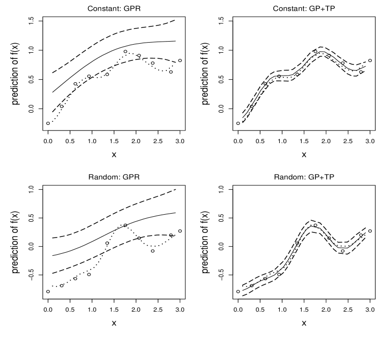
Figure 1: Prediction curves from GPR (the 1st column) and GP-TP (the 2nd column) for data with constant and random disturbances to the 6-th curve, where the circles represent the means of the observed data excluding the 6-th curve, the dotted line stands for the true curve, and solid and dashed lines stand for predicted curves and their 95% confidence bounds.

Now we study performance of the GPR (GP-GP) and GP-TP for batch data with more than one group. We take $I=2$ and $J=6$. Figure 1 plots predictive curves for two sets of simulated data with the constant disturbance of $2.0$ and the random one of $t_{2}+2.0$ respectively. The values of the other parameters are $\phi_{1}=\phi_{2}=0.01$, $\mbox{{\boldmath${\theta}$}${}_{i}$}=(\theta_{i0},\eta_{i1},\xi_{i1})=(0.1,5,0.1),i=1,2$. The upper panel presents the results from the models with constant random disturbances, and the lower panel for the random ones. The disturbance is added to the 6th curve and thus it is an outlying curve. The means for observed data points excluding the 6th curve are computed and represented by circles in the figure. The dotted line stand for the true curve, solid and dashed lines stand for the predicted curve and their 95% point-wise confidence bounds. We see that the prediction from the GP-TP is much closer to the true curve than that from the GPR, indicating that the GP-TP is more robust against outlying curves compared to the GPR.

Table 2 lists simulation study results of MSEs from the two models based on 500 replications, where $\phi_{1}=\phi_{2}=0.2$, $\mbox{{\boldmath${\theta}$}${}_{i}$}=(\theta_{i0},\eta_{i1},\xi_{i1})=(0.1,10,0.1),i=1,2$. It shows that the GP-TP method has smaller value of MSE than the GPR. Especially, the GP-TP performs much better than the GPR for large values of $\gamma$ (1.0 and 2.0).

******Insert Table 2 and Figure 1 here*****

Estimates of the random effects from the GP-TP are presented in Table 3. For the example, there are six independently observed curves and thus six random effects in each group, denoted by $r_{i1}$ to $r_{i6}$, $i=1,2$. We see that $r_{i6}$, which is corresponding to the outlying curve, has much larger value than the others, especially for $\gamma=1.0$ and $2.0$, i.e. large values of $\gamma$. The remaining, $r_{ij}$, $j=1,...,5$, have similar values. From (13), we know that bigger random effects give smaller weight to the corresponding response curve. Hence, the proposed GP-TP is more robust against outlying curves compared to the GPR. In practice, the values of estimated random effects can be used to detect outlying curves, such as the $\hat{r}_{i6}$ shown in Table 3.

******Insert Table 3 here*****

4.2 Real example

Motor learning can be assessed more quickly and robustly than outcomes from rehabilitation. Davison et al. (2014) proposed to utilize a commodity input device to play a bespoke video game to measure the critical components of motor learning. To detect how simple changes in therapist instruction change motor performance and learning, experiment has been conducted by either giving a single objective (single instruction) or by breaking the task down into its two sequential action phases (double instruction). High spatial-temporal resolution data are recorded when participants play a bespoke video game. We then calculate the mean distance between the target and the avatar during the lock and track phase. This index reflects predominantly feedback mechanisms and error correction.

The game data consists of two datasets: 24 young persons and 26 old adults. For each dataset, one half of the subjects received single instruction, saying single treatment group, and the others had twice, denoted by double treatment group. There are $n=180$ mean distances (meandist) recorded for all subjects. The effect of instruction is studied for young and old adult persons, respectively. For each dataset, we separately have two groups, denoted by young with single instruction (young-single), young with double instruction (young-double), old adults with single instruction (old-single), and old adults with double instruction (old-double).

The estimates of random effects in the GP-TP model, $\{r_{i},i=1,...J\}$, are presented in Table 4. We find the estimated random effect for the 4th subject in the young-double group has a much larger value compared to the others, so do the 13th subject in the old-single group. Consequently this model gives small weight to those possible outlying curves and thus reduce their influence on prediction. Table 4 also lists the estimation of random effects after those two curves are deleted ( namely ‘double-4’ and ‘single-13’), showing that the estimation seem to be more regular now.

******Insert Table 4 here*****

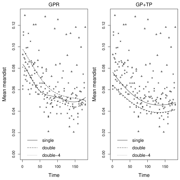
Figure 2: Prediction curves for the young person dataset from GPR and GP-TP models. Cross and circle points represent average values of response meandist of single and double instruction groups respectively, and triangle point stands for meandist of the 4th subject in double instruction group. The solid line stands for the predictive curve of meandist for single instruction group. The dashed and dotted lines stand for the predictions of meandist for double instruction group with and without the 4th subject respectively.

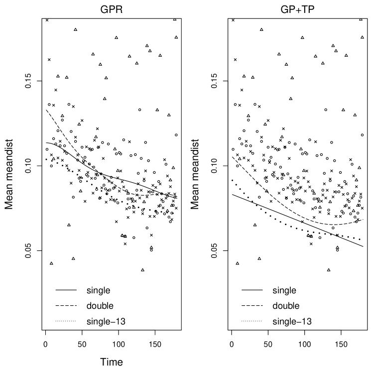
Figure 3: Prediction curves for the old adult dataset from GPR and GP-TP models. Cross and circle points represent average values of response meandist of single and double instruction groups respectively, and triangle point stands for meandist of the 4th subject in double instruction group. The solid and dotted lines stand for the predictive curve of meandist for single instruction group with and without the 13th subject respectively. The dashed line stands for the predictions of meandist for double instruction group.

Prediction curves from the two models are respectively plotted in Figures 2 and 3 for young person and old adult datasets. In both figures, cross and circle points represent average values of meandist for single and double instruction groups respectively, and triangle point stands for meandist of the 4th and 13th subject (outliers). We can see that the 4th subject has larger meandist than the others in young-double subgroup, implying that it may be an outlying curve. The prediction curves in Figure 2 shows that the GP-TP model is almost not affected by the 4th subject, while the affection to the GPR model is quite significant. When the 4th subject is not included in the data set, the predicted values for the double group calculated from the GPR are almost the same as the ones from the single group in the area of the first half, but the GP-TP model shows the difference uniformly in the whole area no matter whether the 4th subject is included or not. This shows the property of robustness of the GP-TP model. Figure 3 shows a similar result.

******Insert Figures 2 and 3 here*****

5 Concluding remarks

This paper develops a robust estimation procedure via h-likelihood for an independent error model with functional batch data. The estimated random effects are useful to detect outlying curves. Unbiasness and information consistency are shown. Numerical studies show that the proposed estimation procedure is robust against outlying curves, and has a better performance in the presence of outliers compared to the GPR and eTPR models. We focused our discussion in this paper on the TP+TP model, but the estimation procedure can be applied straightly to other types of models, for example, functional regression models with independent errors of multivariate t distribution (MVT). In this case, model (9) is modified as: $f_{i}\sim GP(k_{i})$, $\epsilon_{ijk}\sim MVT(\nu_{1},\phi_{i})$, for $i=1,...,I,j=1,...,J,k=1,...,n$, where $f_{i}$ and $\epsilon_{ijk}$ are independent. The errors can be defined equivalently to

$$\epsilon_{ijk}|r_{ijk}\sim N(0,r_{ijk}\phi_{i}),~{}~{}r_{ijk}\sim\mathrm{{IG}(\nu_{1},\nu_{1}-1)}.$$

Thus we can use the h-likelihood method given in Section 3 to estimate the unknown function $f_{i}$.

In addition, the proposed method can be extended to generalized linear model with functional data.

Appendix

Hereafter, let $c$ be any positive constant independent of $n$, which may

stands for various

values in different places. Without loss of generality, firstly we set $I=J=1$ which is the situation in Section 2. Let $p_{\phi_{0}}(\mbox{{\boldmath${y}$}}|f_{0},\mbox{{\boldmath${X}$}})$ be the density function to generate the data ${y}$ given ${X}$ under the true model (1), where $f_{0}$ is the true underlying function of $f$. Let $p_{\theta,r}(f)$ be a measure of random process $f$ on space ${\mathcal{F}}=\{f(\cdot):\mathcal{X}\rightarrow R\}$ for given random effect ${r}$. Let

$$p_{\phi,\theta,r}(\mbox{{\boldmath${y}$}}|\mbox{{\boldmath${X}$}})=\int_{{\mathcal{F}}}p_{\phi,r}(\mbox{{\boldmath${y}$}}|f,\mbox{{\boldmath${X}$}})dp_{\theta,r}(f),$$

be the density function to generate the data ${y}$ given ${X}$ under the assumed model (2) and given ${r}$. Here $\phi$ is the common parameter in both models and let $\phi_{0}$ be the true value of $\phi$. Let $p_{\phi_{0},\hat{\theta},\hat{r}}(\mbox{{\boldmath${y}$}}|\mbox{{\boldmath${X}$}})$ be the estimated density function under the assumed model (2). Before proving Theorem 1, we need the following Lemma.

Lemma 1 Suppose $\mbox{{\boldmath${y}$}}=\{y_{1},...,y_{n}\}$ are generated from model (2) with the mean function $h(\mbox{\boldmath${x}$})=0$, and covariance kernel function $k$ is bounded and continuous in parameter ${\theta}$. It also assumes that the estimate $\hat{\mbox{\boldmath${\beta}$}}$ and $\hat{\mbox{\boldmath${r}$}}$ are consistent estimators of ${\beta}$ and ${r}$, respectively. Then for any $\varepsilon>0$, when $n$ is large enough, we have

$$\frac{1}{n}(-\log p_{\phi_{0},\hat{\theta},\hat{r}}(\mbox{{\boldmath${y}$}$$}|\mbox{{\boldmath${X}$}$$})+\log p_{\phi_{0}}(\mbox{{\boldmath${y}$}$$}|f_{0},\mbox{{\boldmath${X}$}$$}))$$

$$\leq \frac{1}{2n}\Big{\{}\int\log|\mbox{{\boldmath${I}$}${}_{n}$}+r_{0}\mbox{{\boldmath${K}$}${}_{n}$}/(r_{1}\phi_{0})|g_{\nu_{0}}(r_{0})g^{*}_{\nu_{1}}(r_{1})dr_{0}dr_{1}+||f_{0}||^{2}_{k}+c\Big{\}}+\varepsilon,$$

where $\mbox{{\boldmath${K}$}${}_{n}$}=(k(\mbox{{\boldmath${x}$}${}_{j}$},\mbox{{\boldmath${x}$}${}_{l}$}))_{n\times n}$, ${I}$_n is the $n\times n$ identity matrix, $||f_{0}||_{k}$ is the reproducing kernel Hilbert space norm of $f_{0}$ associated with kernel function $k(\cdot,\cdot;\mbox{\boldmath${\theta}$})$, ${g}_{\nu_{0}}(\cdot)$ and ${g}_{\nu_{1}}^{*}(\cdot)$ are the density functions of $IG(\nu_{0},\nu_{0}-1)$ and $IG(\nu_{1}+n/2,(\nu_{1}-1)+q^{2}/2)$, respectively, and $q^{2}=(\mbox{{\boldmath${y}$}$$}-f_{0}(\mbox{{\boldmath${X}$}$$}))^{T}(\mbox{{\boldmath${y}$}$$}-f_{0}(\mbox{{\boldmath${X}$}$$}))/\phi_{0}$.

Proof: Suppose that for any given $\mbox{\boldmath${r}$}=(r_{0},r_{1})^{T}$, we have

$$-\log p_{\phi_{0},\theta,r}(\mbox{{\boldmath${y}$}$$}|\mbox{{\boldmath${X}$}$$})+\log p_{\phi_{0},r}(\mbox{{\boldmath${y}$}$$}|f_{0},\mbox{{\boldmath${X}$}$$}))$$

$$\leq \frac{1}{2}\log|\mbox{{\boldmath${I}$}${}_{n}$}+r_{0}\mbox{{\boldmath${K}$}${}_{n}$}/(r_{1}\phi_{0})|+\frac{r_{0}}{2}(||f_{0}||^{2}_{k}+c)+c+n\varepsilon.$$ (A.1 )

Let $\hat{\mbox{\boldmath${r}$}}$ and $\tilde{\mbox{\boldmath${r}$}}$ be maximizers of functions $\log p_{\phi_{0},\theta,r}(\mbox{\boldmath${y}$}|\mbox{\boldmath${X}$})+\log f_{\nu}(\mbox{\boldmath${r}$})$ and $\log p_{\phi_{0},\theta,r}(\mbox{\boldmath${y}$}|\mbox{\boldmath${X}$})$, respectively, where $f_{\nu}(\mbox{\boldmath${r}$})=g_{\nu_{0}}(r_{0})g_{\nu_{1}}(r_{1})$. We have

$$1\leq\frac{\log p_{\phi_{0},\theta,\tilde{r}}(\mbox{\boldmath${y}$}|\mbox{\boldmath${X}$})}{\log p_{\phi_{0},\theta,\hat{r}}(\mbox{\boldmath${y}$}|\mbox{\boldmath${X}$})}\leq 1+\frac{\log f_{\nu}(\hat{\mbox{\boldmath${r}$}})-\log f_{\nu}(\tilde{\mbox{\boldmath${r}$}})}{\log p_{\phi_{0},\theta,\hat{r}}(\mbox{\boldmath${y}$}|\mbox{\boldmath${X}$})},$$

which indicates that

$$p_{\phi_{0},\theta,\tilde{r}}(\mbox{\boldmath${y}$}|\mbox{\boldmath${X}$})\leq p_{\phi_{0},\theta,\hat{r}}(\mbox{\boldmath${y}$}|\mbox{\boldmath${X}$})^{1+\varepsilon},$$

because $f_{\nu}(\mbox{\boldmath${r}$})$ is independent of $n$ while $\log p_{\phi_{0},\theta,\hat{r}}(\mbox{\boldmath${y}$}|\mbox{\boldmath${X}$})$ tends to infinity as $n$ goes to $\infty$. Thence,

$$\int p_{\phi_{0},\theta,r}(\mbox{\boldmath${y}$}|\mbox{\boldmath${X}$})f_{\nu}(\mbox{\boldmath${r}$})d\mbox{\boldmath${r}$}\leq p_{\phi_{0},\theta,\hat{r}}(\mbox{\boldmath${y}$}|\mbox{\boldmath${X}$})^{1+\varepsilon}.$$ (A.2 )

By simple computation, we show that

$$\int p_{\phi_{0},r}(\mbox{\boldmath${y}$}|f_{0},\mbox{\boldmath${X}$})\exp\{-(\frac{1}{2}\log|\mbox{{\boldmath${I}$}${}_{n}$}+r_{0}\mbox{{\boldmath${K}$}${}_{n}$}/(r_{1}\phi_{0})|+\frac{r_{0}}{2}(||f_{0}||^{2}_{k}+c))\}f_{\nu}(\mbox{\boldmath${r}$})d\mbox{\boldmath${r}$}$$

$$= p_{\phi_{0}}(\mbox{\boldmath${y}$}|f_{0},\mbox{\boldmath${X}$})\int\exp\{-(\frac{1}{2}\log|\mbox{{\boldmath${I}$}${}_{n}$}+r_{0}\mbox{{\boldmath${K}$}${}_{n}$}/(r_{1}\phi_{0})|+\frac{r_{0}}{2}(||f_{0}||^{2}_{k}+c))\}$$

$$g_{\nu_{0}}(r_{0})g^{*}_{\nu_{1}}(r_{1})dr_{0}dr_{1}.$$ (A.3 )

From (Appendix), (A.2) and (Appendix), we have

$$\frac{1}{n}(-\log p_{\phi_{0},\theta,\hat{r}}(\mbox{{\boldmath${y}$}$$}|\mbox{{\boldmath${X}$}$$})+\log p_{\phi_{0}}(\mbox{{\boldmath${y}$}$$}|f_{0},\mbox{{\boldmath${X}$}$$}))$$

$$\leq -\frac{1}{n}\log\Big{\{}\int\exp\{-(\frac{1}{2}\log|\mbox{{\boldmath${I}$}${}_{n}$}+r_{0}\mbox{{\boldmath${K}$}${}_{n}$}/(r_{1}\phi_{0})|+\frac{r_{0}}{2}(||f_{0}||^{2}_{k}+c))\}$$

$$g_{\nu}(r_{0})g^{*}_{\nu}(r_{1})dr_{0}dr_{1}\Big{\}}+\varepsilon$$

$$\leq \frac{1}{2n}\Big{\{}\int\log|\mbox{{\boldmath${I}$}${}_{n}$}+r_{0}\mbox{{\boldmath${K}$}${}_{n}$}/(r_{1}\phi_{0})|g_{\nu}(r_{0})g^{*}_{\nu}(r_{1})dr_{0}dr_{1}+||f_{0}||^{2}_{k}+c\Big{\}}+\varepsilon,$$

which shows that Lemma 1 holds.

Now let us prove the inequality (Appendix). Following proofs of Theorem 1 in Seeger et al. (2008) and Lemma 1 in Wang and Shi (2014), it is sufficient to prove (Appendix) when the true underlying function has the expression

$${f}_{0}(\cdot)=r_{0}\sum_{l=1}^{n}\alpha_{l}k(\mbox{\boldmath${x}$},\mbox{{\boldmath${x}$}${}_{i}$};\mbox{{\boldmath${\theta}$}$$})\doteq r_{0}K(\cdot)\mbox{\boldmath${\alpha}$},$$

where $K(\cdot)=(k(\mbox{\boldmath${x}$},\mbox{{\boldmath${x}$}${}_{1}$};\mbox{{\boldmath${\theta}$}$$}),...,k(\mbox{\boldmath${x}$},\mbox{{\boldmath${x}$}${}_{n}$};\mbox{{\boldmath${\theta}$}$$}))$ and $\mbox{\boldmath${\alpha}$}=(\alpha_{1},...,\alpha_{n})^{T}\in R^{n}$.

Let $P$ be a measure induced by $GP(0,r_{0}k(\cdot,\cdot;\hat{\mbox{\boldmath${\theta}$}}))$. Let $Q$ be the density function of normal distribution $N(f_{0}(\mbox{\boldmath${X}$}),r_{0}\mbox{{\boldmath${K}$}${}_{n}$}(r_{0}\mbox{{\boldmath${K}$}${}_{n}$}/(r_{1}\phi_{0})+\mbox{{\boldmath${I}$}${}_{n}$})^{-1})$. We can show that $Q$ is the posterior distribution of $\tilde{f}$ from a model with prior $GP(0,r_{0}k(\cdot,\cdot;\mbox{{\boldmath${\theta}$}$$}))$ and Gaussian likelihood term $\prod_{l=1}^{n}N(\hat{y}_{i}|\tilde{f}(\mbox{{\boldmath${x}$}${}_{i}$}),r_{1}\phi_{0})$, where $\hat{\mbox{\boldmath${y}$}}=(\hat{y}_{1},...,\hat{y}_{n})^{T}=(r_{0}\mbox{{\boldmath${K}$}${}_{n}$}+r_{1}\phi_{0}\mbox{{\boldmath${I}$}${}_{n}$})\mbox{\boldmath${\alpha}$}$. Then we have $E_{Q}(\tilde{f})=f_{0}$, where the expectation is taken under probability density $Q$. From Fenchel-Legendre duality relationship in Boyd and Vandenberghe (2002) and Rockafellar (1970), we have

$$-\log p_{\phi_{0},\theta,r}(\mbox{{\boldmath${y}$}$$}|\mbox{{\boldmath${X}$}$$})\leq E_{Q}(-\log p_{\phi_{0},r}(\mbox{{\boldmath${y}$}$$}|\tilde{f},\mbox{{\boldmath${X}$}$$})+D[Q,P].$$ (A.4 )

Let $\mbox{\boldmath${B}$}=\mbox{{\boldmath${I}$}${}_{n}$}+r_{0}\mbox{{\boldmath${K}$}${}_{n}$}/(r_{1}\phi_{0})$, then we have

$$D[Q,P]=\frac{1}{2}\left\{-\log|\hat{\mbox{\boldmath${K}$}}_{n}^{-1}\mbox{{\boldmath${K}$}${}_{n}$}|+\log|\mbox{\boldmath${B}$}|+Tr(\hat{\mbox{\boldmath${K}$}}_{n}^{-1}\mbox{{\boldmath${K}$}${}_{n}$}\mbox{{\boldmath${B}$}${}^{-1}$})\right.$$

$$\hskip 56.9055pt\left.+r_{0}||f_{0}||^{2}_{k}+r_{0}\mbox{\boldmath${\alpha}$}\mbox{{\boldmath${K}$}${}_{n}$}(\hat{\mbox{\boldmath${K}$}}_{n}^{-1}\mbox{{\boldmath${K}$}${}_{n}$}-\mbox{{\boldmath${I}$}${}_{n}$})\mbox{\boldmath${\alpha}$}-n\right\},$$ (A.5 )

$$E_{Q}(-\log p_{\phi_{0},r}(\mbox{{\boldmath${y}$}$$}|\tilde{f},\mbox{\boldmath${X}$}))$$

$$\leq -\log p_{\phi_{0},r}(\mbox{{\boldmath${y}$}$$}|f_{0},\mbox{\boldmath${X}$}))+\frac{r_{0}}{2r_{1}\phi_{0}}Tr(\mbox{{\boldmath${K}$}${}_{n}$}\mbox{{\boldmath${B}$}${}^{-1}$}),$$ (A.6 )

where $\hat{\mbox{\boldmath${K}$}}_{n}=(k(\mbox{{\boldmath${x}$}${}_{j}$},\mbox{{\boldmath${x}$}${}_{l}$};\hat{\mbox{\boldmath${\theta}$}}))_{n\times n}$.

From (A.4), (A.5) and (A.6), it gives that

$$-\log p_{\phi_{0},\theta,r}(\mbox{{\boldmath${y}$}$$}|\mbox{{\boldmath${X}$}$$})+\log p_{\phi_{0},r}(\mbox{{\boldmath${y}$}$$}|f_{0},\mbox{\boldmath${X}$}))$$

$$\leq \frac{1}{2}\left\{-\log|\hat{\mbox{\boldmath${K}$}}_{n}^{-1}\mbox{{\boldmath${K}$}${}_{n}$}|+\log|\mbox{\boldmath${B}$}|+Tr((\hat{\mbox{\boldmath${K}$}}_{n}^{-1}\mbox{{\boldmath${K}$}${}_{n}$}+r_{0}\mbox{{\boldmath${K}$}${}_{n}$}/(r_{1}\phi_{0}))\mbox{{\boldmath${B}$}${}^{-1}$})+r_{0}||f_{0}||^{2}_{k}\right.$$

$$\left.+r_{0}\mbox{\boldmath${\alpha}$}\mbox{{\boldmath${K}$}${}_{n}$}(\hat{\mbox{\boldmath${K}$}}_{n}^{-1}\mbox{{\boldmath${K}$}${}_{n}$}-\mbox{{\boldmath${I}$}${}_{n}$})\mbox{\boldmath${\alpha}$}-n\right\}.$$ (A.7 )

Due to the bounded, continuous covariance function and almost sure convergence of $\hat{\mbox{\boldmath${\theta}$}}$, we have $\hat{\mbox{\boldmath${K}$}}_{n}^{-1}\mbox{{\boldmath${K}$}${}_{n}$}-\mbox{{\boldmath${I}$}${}_{n}$}\rightarrow 0$ as $n\rightarrow\infty$. Hence, there exist positive constants $c$ and $\varepsilon$ such that for a large enough $n$

$$-\log|\hat{\mbox{\boldmath${K}$}}_{n}^{-1}\mbox{{\boldmath${K}$}${}_{n}$}|<c,~{}~{}\mbox{\boldmath${\alpha}$}\mbox{{\boldmath${K}$}${}_{n}$}(\hat{\mbox{\boldmath${K}$}}_{n}^{-1}\mbox{{\boldmath${K}$}${}_{n}$}-\mbox{{\boldmath${I}$}${}_{n}$})\mbox{\boldmath${\alpha}$}<c,$$

$$Tr(\hat{\mbox{\boldmath${K}$}}_{n}^{-1}\mbox{{\boldmath${K}$}${}_{n}$}\mbox{{\boldmath${B}$}${}^{-1}$})<Tr((\mbox{{\boldmath${I}$}${}_{n}$}+\varepsilon\mbox{{\boldmath${K}$}${}_{n}$})\mbox{{\boldmath${B}$}${}^{-1}$}).$$ (A.8 )

Plugging (Appendix) in (Appendix), we have the inequality (Appendix). $\sharp$

Under condition
(A) $||f_{0i}||_{k}$ is bounded and $E_{\mbox{{\boldmath${X}$}${}_{i}$}}(\log|\mbox{{\boldmath${I}$}${}_{n}$}+c\mbox{{\boldmath${K}$}${}_{in}$}|)=o(n)$ for any $c>0$ and $i=1,...,I$,
it follows from Lemma 1 that for $I=J=1$,

$$\frac{1}{n}E_{\mbox{{\boldmath${X}$}$$}}(D[p_{\phi_{0}}(\mbox{{\boldmath${y}$}$$}|f_{0},\mbox{{\boldmath${X}$}$$}),p_{\phi_{0},\hat{\theta},\hat{r}}(\mbox{{\boldmath${y}$}$$}|\mbox{{\boldmath${X}$}$$})])\longrightarrow 0,{\mbox{as}}~{}~{}n\rightarrow\infty.$$ (A.9 )

Proof of Theorem 1: Suppose $\mbox{{\boldmath${y}$}${}_{i}$}=\{y_{i1},...,y_{in}\}$ are generated from model (9) with the mean function $h(\mbox{\boldmath${x}$})=0$, and covariance kernel $k_{i}$ is bounded and continuous in parameter ${\theta}$_i. Under condition (A), similar to proof of (A.9), we show that

$$\frac{1}{n}E_{\mbox{{\boldmath${X}$}${}_{i}$}}(D[p_{\phi_{0i}}(\mbox{{\boldmath${y}$}${}_{i}$}|f_{0i},\mbox{{\boldmath${X}$}${}_{i}$}),p_{\phi_{0i},\hat{\theta}_{i},\hat{r}_{i}}(\mbox{{\boldmath${y}$}${}_{i}$}|\mbox{{\boldmath${X}$}${}_{i}$})])\longrightarrow 0,{\mbox{as}}~{}~{}n\rightarrow\infty.$$

Hence, Theorem 1 holds.$\sharp$

References

Table 1: MSEs and standard deviations (in parentheses) of the predictions from GPR, eTPR and GP-TP

Error	Disturbance	$\gamma$	GPR	eTPR	GP-TP
Gaussian	constant	0.5	0.038(0.022)	0.038(0.022)	0.037(0.021)
		1.0	0.060(0.027)	0.060(0.028)	0.038(0.021)
		2.0	0.145(0.052)	0.145(0.053)	0.044(0.027)
Gaussian	random	0.5	0.157(0.394)	0.156(0.391)	0.047(0.118)
		1.0	0.177(0.536)	0.177(0.536)	0.044(0.029)
		2.0	0.225(0.425)	0.225(0.426)	0.051(0.049)
ETP($\nu=2.0$)	constant	0.5	0.049(0.033)	0.049(0.032)	0.040(0.028)
		1.0	0.072(0.044)	0.072(0.044)	0.047(0.033)
		2.0	0.150(0.066)	0.151(0.066)	0.050(0.035)
ETP($\nu=1.0$)	constant	0.5	0.089(0.155)	0.089(0.157)	0.048(0.034)
		1.0	0.093(0.081)	0.093(0.082)	0.055(0.043)
		2.0	0.167(0.126)	0.167(0.126)	0.058(0.045)

Table 2: MSEs and standard deviations (in parentheses) of the predictions from GPR and GP-TP, where the error term has Gaussian distribution

Disturbance	$\gamma$	GPR	GP-TP
constant	0.5	0.037(0.015)	0.036(0.015)
	1.0	0.061(0.020)	0.040(0.017)
	2.0	0.144(0.037)	0.051(0.026)
random	0.5	0.276(1.212)	0.045(0.042)
	1.0	0.182(0.407)	0.048(0.049)
	2.0	4.364(92.235)	0.052(0.036)

Table 3: Estimation of random effects $r_{ij}$ and their standard deviations (in parentheses) from GP-TP for $i=1,2$ and $j=1,..,6$.

Disturbance	$\gamma$	$r_{11}$	$r_{12}$	$r_{13}$	$r_{14}$	$r_{15}$	$r_{16}$
constant	0.5	0.534(0.284)	0.531(0.284)	0.536(0.285)	0.554(0.295)	0.539(0.288)	0.819(0.433)
	1.0	0.313(0.278)	0.318(0.280)	0.315(0.279)	0.311(0.273)	0.319(0.289)	1.113(0.969)
	2.0	0.233(0.209)	0.235(0.213)	0.232(0.208)	0.23(0.204)	0.234(0.206)	2.553(2.107)
random	0.5	0.357(0.292)	0.367(0.295)	0.349(0.284)	0.353(0.285)	0.356(0.289)	3.707(20.884)
	1.0	0.313(0.291)	0.310(0.284)	0.308(0.289)	0.318(0.298)	0.303(0.284)	2.187(5.027)
	2.0	0.254(0.244)	0.258(0.252)	0.255(0.251)	0.254(0.241)	0.255(0.242)	4.019(17.145)
		$r_{21}$	$r_{22}$	$r_{23}$	$r_{24}$	$r_{25}$	$r_{26}$
constant	0.5	0.549(0.29)	0.548(0.297)	0.525(0.276)	0.545(0.3)	0.537(0.292)	0.855(0.456)
	1.0	0.315(0.281)	0.319(0.286)	0.319(0.285)	0.328(0.296)	0.322(0.289)	1.121(0.975)
	2.0	0.236(0.208)	0.229(0.204)	0.238(0.21)	0.229(0.201)	0.227(0.202)	2.618(2.145)
random	0.5	0.369(0.313)	0.371(0.299)	0.362(0.302)	0.362(0.293)	0.364(0.298)	3.447(30.013)
	1.0	0.317(0.297)	0.316(0.301)	0.304(0.279)	0.311(0.298)	0.305(0.279)	2.753(11.809)
	2.0	0.251(0.241)	0.25(0.241)	0.243(0.231)	0.25(0.24)	0.25(0.245)	4.193(15.459)

Table 4: Estimation of random effects from GP-TP for the game data

group	instruction	r1	r2	r3	r4	r5	r6	r7	r8	r9	r10	r11	r12	r13
Young	single	0.183	0.569	0.264	0.379	0.369	0.460	1.016	0.281	0.367	0.206	0.280	0.450
	double	0.161	0.787	0.366	9.472	0.796	0.310	1.373	0.259	0.147	0.101	0.133	1.051
	double-4	0.309	1.529	0.710	-	1.546	0.609	2.655	0.507	0.274	0.195	0.251	2.040
Old	single	0.092	0.241	0.767	0.238	0.063	0.719	0.288	0.143	0.172	0.294	1.115	0.952	5.193
	double	0.268	0.205	1.335	2.192	0.450	0.135	0.213	1.303	0.131	0.146	0.227	0.147	0.371
	single-13	0.169	0.463	1.488	0.464	0.116	1.410	0.546	0.263	0.319	0.561	2.159	1.868	-

References

- Boyd and Vandenberghe (2002) Boyd S. and Vandenberghe L. (2002), Convex Optimization. Cambridge University Press.
- Cao et al. (2017) Cao, C., Shi, J. Q. and Lee, Y. (2017). Robust functional regression model for population-average and subject-specific inferences. Statistical Methods in Medical Research, (to appear). arXiv:1705.05618.
- Choi and Schervish (2007) Choi, T. and Schervish, M.J. (2007). On posterior consistency in nonparametric regression problems. J. Multivariate Analysis, 98, 1969-87.
- Davison et al. (2014) Davison R, Graziadio S, Shalabi K, Ushaw G, Morgan G, Eyre J. (2014). Early response markers from video games for rehabilitation strategies. ACM SIGAPP Applied Computing Review, 14(3), 36-43.
- Gramacy and Lian (2012) Gramacy, R. and Lian, H. (2012), Gaussian process single-index models as emulators for computer experiments, Technometrics, 54, 30 - 41.
- Kackar and Harville (1984) Kackar, R.N. and Harville, D.A. (1984). Approximations for standard errors of estimators of fixed and random effects in mixed linear models. Journal of the American Statistical Association: 79: 853-862.
- Lee and Kim (2016) Lee, Y. and Kim, G. (2016). H-likelihood predictive intervals for unobservables, International Statistical Review, DOI: 10.1111/insr.12115.
- Lee and Nelder (1996) Lee, Y. and Nelder, J.A. (1996). Hierarchical Generalized Linear Models. Journal of the Royal Statistical Society B, 58, 619-678.
- Lee and Nelder (2006) Lee, Y. and Nelder, J.A. (2006). Double hierarchical generalized linear models (with discussion). Journal of the Royal Statistical Society: C (Applied Statistics), 55, 139-185.
- Lee et al. (2006) Lee, Y., Nelder, J.A. and Pawitan, Y. (2006). Generalized Linear Models with Random Effects, Unified Analysis via H-likelihood. Chapman & Hall/CRC.
- Paik et al. (2015) Paik, M. C., Lee, Y., Ha, I. D. (2015). Frequentist inference on random effiects based on summarizability. Statistica. Sinica 25, 1107-1132.
- Rockafellar (1970) Rockafellar R. (1970), Convex Analysis. Princeton University Press.
- Rasmussen and Williams (2006) Rasmussen, C. E. and Williams, C. K. I. (2006), Gaussian Processes for Machine Learning. Cambridge, Massachusetts: The MIT Press.
- Shah et al. (2014) Shah A., Wilson A.G. and Ghahramani Z. (2014). Student-t processes as alternatives to Gaussian processes. Proceedings of the 17th International Conference on Artificial Intelligence and Statistics (AISTATS), 877-885.
- Shi and Choi (2011) Shi, J. Q. and Choi, T. (2011). Gaussian Process Regression Analysis for Functional Data, London: Chapman and Hall/CRC.
- Seeger et al. (2008) Seeger M. W., Kakade S. M. and Foster D. P. (2008). Information Consistency of Nonparametric Gaussian Process Methods, IEEE Transactions on Information Theory, 54, 2376-2382.
- Shi et al. (2007) Shi, J. Q., Wang, B., Murray-Smith, R. and Titterington, D. M. (2007), Gaussian Process Functional Regression Modelling for Batch Data, Biometrics, 63, 714-723.
- Wang and Shi (2014) Wang, B. and Shi, J.Q. (2014). Generalized Gaussian process regression model for non-Gaussian functional data. Journal of the American Statistical Association, 109, 1123-1133.
- Wang et al. (2017) Wang, Z, Shi, J. Q. and Lee, Y. (2015). Extended T-process Regression Models. Journal of Statistical Planning and Inference, (to appear). arXiv:1705.05125
- Xu et al. (2011) Xu, Z., Yan, F. and Qi, Y. (2011), Sparse Matrix-Variate t Process Blockmodel. Proceedings of the 25th AAAI Conference on Artificial Intelligence, 543-548.
- Yu et al. (2007) Yu S., Tresp V. and Yu K. (2007), Robust multi-tast learning with t-process. Proceedings of the 24th International Conference on Machine Learning, 1103-1110.
- Zhang and Yeung (2010) Zhang, Y. and Yeung, D.Y. (2010), Multi-task learning using generalized process. Proceedings of the 13th International Conference on Artificial Intelligence and Statistics (AISTATS), 964-971.