Solitary waves in the Nonlinear Dirac Equation

Abstract

In the present work, we consider the existence, stability, and dynamics of solitary waves in the nonlinear Dirac equation. We start by introducing the Soler model of self-interacting spinors, and discuss its localized waveforms in one, two, and three spatial dimensions and the equations they satisfy. We present the associated explicit solutions in one dimension and numerically obtain their analogues in higher dimensions. The stability is subsequently discussed from a theoretical perspective and then complemented with numerical computations. Finally, the dynamics of the solutions is explored and compared to its non-relativistic analogue, which is the nonlinear Schrödinger equation. A few special topics are also explored, including the discrete variant of the nonlinear Dirac equation and its solitary wave properties, as well as the $\mathcal{P}\mathcal{T}$-symmetric variant of the model.

1 Introduction

In the last three decades, there has been an enormous interest in the study of waves in nonlinear dispersive media. Arguably, two of the most paradigmatic equations that describe such waves are the nonlinear Schrödinger equation (NLS) and the sine–Gordon equation. The first among these equations covers a broad range of settings including atomic physics cuevas-PS03 ; cuevas-PS02 , nonlinear optics cuevas-KFC15 ; cuevas-KA03 , condensed matter physics, and mathematical physics cuevas-APT04 ; cuevas-SS99 . The sine–Gordon equation also covers settings in condensed matter physics and mathematical physics apart from high-energy physics models cuevas-BK04 ; cuevas-CKW14 . A principal focus of the relevant properties of these equations has been the study of the existence, stability, and dynamics of solitary waves (i.e. spatially localized waves supported by the nonlinearity and dispersion), both in lower-dimensional settings (such as one-dimensional solitons and multi-solitons) and in higher dimensional settings (vortices, vortex rings, and related structures) cuevas-DP06 ; cuevas-KFC15 .

By comparison, far less attention has been paid to the nonlinear Dirac equation (NLD), despite its presence for almost 90 years in the realm of high energy physics. The nonlinear Dirac equation with scalar-type self-interaction was initially introduced by Ivanenko in 1938 cuevas-Iva38 . Following the ideas of Finkelstein cuevas-FLR51 , Heisenberg in 1957 cuevas-Hei57 used this NLD model in an attempt to formulate a unified theory of elementary particles. In 1958, a completely integrable one-dimensional model known as the Massive Thirring Model (MTM) cuevas-Thi58 , based on vector-type self-interaction of spinor field, was introduced. This model possesses solitary wave solutions. Curiously, fundamental solutions of the MTM can be transformed into solitons of the sine–Gordon equation by means of a bosonization process cuevas-Col75 . In 1970, Soler re-introduced Ivanenko’s model with scalar-type self-interaction in the context of extended nucleons cuevas-Sol70 and also provided the numerical analysis of solitary wave solutions. The one-dimensional version of the Soler model, known as the Gross–Neveu model cuevas-GN74 , was introduced in 1974 as a toy model of quark confinement in quantum chromodynamics, and explicit solitary wave solutions in the corresponding massive model were found by Lee et al. in 1975 cuevas-LKG75 . We can not complete this quick review of NLD models in high-energy physics without mentioning the recent work of cuevas-NP09 (see also cuevas-MLB14 ), where a variant of the NLD is applied to the study of neutrino oscillations. Related systems are the Dirac–Maxwell system cuevas-Gro66 ; cuevas-Wak66 ; cuevas-Bou96 ; cuevas-EGS96 ; cuevas-CS12 , the Einstein–Dirac system cuevas-Rot10a ; cuevas-Stu10 , and Einstein–Dirac–Maxwell system cuevas-Rot10 . In quantum chemistry, the Dirac–Hartree–Fock model cuevas-LM82 ; cuevas-ES99 ; cuevas-ES01 takes into account the fermionic properties of electrons (describing the exchange interaction, which is a fundamental effect of purely quantum nature) and is used for accurate computation of the electronic energy cuevas-VD97 ; cuevas-QGW04 ; this model has also started to receive mathematical attention cuevas-ES99 ; cuevas-ES01 ; cuevas-ES05 .

Recent years have seen a gradual increase of interest in the study of near-relativistic settings, arguably, for three principal reasons. Firstly, significant steps have been taken in the nonlinear analysis of stability of such models cuevas-BC12 ; cuevas-PS14 ; cuevas-BC16a , especially in one-dimensional cuevas-PS12 ; cuevas-CPS17 ; cuevas-BC12a ; cuevas-BC16a and two-dimensional settings cuevas-CKS+16a . Secondly, computational advances have enabled a better understanding of the associated solitary wave solutions and their dynamics cuevas-XST13 ; cuevas-CKMS10 ; cuevas-SQM+14 ; cuevas-CKS15 also in the presence of external fields cuevas-MQC+12 . Thirdly, and perhaps most importantly, NLD starts emerging in physical systems which arise in a diverse set of contexts of considerable interest. These contexts include, in particular, bosonic evolution in honeycomb lattices cuevas-HOC15 ; cuevas-HC15a and a growing class of atomically thin 2D Dirac materials cuevas-WBB14 ; cuevas-FSL+17 such as graphene, silicene, germanene, borophene, and transition metal dichalcogenides cuevas-MLH+10 . Recently, the physical aspects of nonlinear optics, such as light propagation in honeycomb photorefractive lattices (the so-called photonic graphene) cuevas-ANZ09 ; cuevas-AZ10 have prompted the consideration of intriguing dynamical features, e.g. conical diffraction in 2D honeycomb lattices cuevas-PBF+07 . Inclusion of nonlinearity is then quite natural in these models, although in a number of them (e.g., in atomic and optical physics) the nonlinearity does not couple the spinor components and breaks the Lorentz symmetry (that is, such models are not invariant under Lorentz transformations; for the explicit form of the Lorentz transformations of the spinor fields see e.g. cuevas-BD64 ; cuevas-Tha92 ).

It would be relevant to mention one more framework where Dirac-type equations have received significant attention in recent years, that is in the context of spin-orbit coupled Bose–Einstein condensates cuevas-DGJO11 . There, admittedly, the setup is somewhat different, as both the Dirac type operator and the Schrödinger one co-exist, but it is relevant to point out that such settings have already been realized experimentally cuevas-LBJ+13 ; cuevas-LJS11 ; cuevas-QHG+13 . Moreover, a wide range of coherent structures has been already proposed in them including vortices cuevas-RSSG11 ; cuevas-ROL+12 ; cuevas-XH11 , Skyrmions cuevas-KMNM12 , Dirac monopoles cuevas-Con12 , and dark solitons cuevas-ASK+13 ; cuevas-FBZ12 , as well as self-trapped states cuevas-MJZ+10 , bright solitons cuevas-AFKP13 ; cuevas-XZW13 , and gap-solitons cuevas-KKA13 . It has also been demonstrated that in such systems it is possible to create stable vortex solitons in free space, which until recently was considered impossible due to the presence of collapse, driven by the self-attractive cubic nonlinearity cuevas-SLM14 .

From a mathematical perspective, Dirac models are described by systems (rather than by scalar equations) that correspond to the Hamiltonian functionals unbounded from below. This unboundedness makes all the aspects of the analysis of these models (well-posedness, existence of localized solutions, stability, numerical simulations) much more challenging. This has fueled an increasing interest in the nonlinear Dirac equation and more general models of self-interacting spinor fields, with many results on the existence of solitary waves cuevas-CV86 ; cuevas-Mer88 ; cuevas-ES95 and well-posedness in (3+1)D cuevas-EV97 ; cuevas-MNNO05 and in (1+1)D cuevas-ST10 ; cuevas-MNT10 ; cuevas-Can11 ; cuevas-Pel11a ; cuevas-Huh13 . The stability of solitary wave solutions of the nonlinear Dirac equation was approached via numerical simulations cuevas-RRSV74 ; cuevas-AS83 ; cuevas-AS86 ; cuevas-BPZ98 ; cuevas-CP06 ; cuevas-BC12a ; cuevas-MQC+12 ; cuevas-XST13 and via heuristic arguments cuevas-Bog79 ; cuevas-MM86 ; cuevas-SV86 ; cuevas-BSV87 ; cuevas-CKMS10 , but it is still not settled. Recently, the first stability results in the context of self-interacting spinor fields started appearing cuevas-Bou06 ; cuevas-Bou08 ; cuevas-BC12a ; cuevas-PS14 ; cuevas-BC16a ; cuevas-CPS17 ; cuevas-BC17 .

The NLD can also be viewed as a relativistic generalization (or extension) of the NLS, or, alternatively, the NLS (with additional terms) can be seen as a special case limit of the NLD at the low-energy limit. Nevertheless, it has turned out that the Dirac equation as a result of its matrix nature and the fact that it is only first order in spatial derivatives (as opposed to second order in the NLS) has proven far more computationally (and theoretically) challenging, on a number of grounds, than its NLS counterpart. This difficulty has hindered the progress in the study of solitary waves, particularly in two-dimensional and three-dimensional settings. However, recent developments are gradually enabling the study of the stability and dynamical properties of solitary waves in two-dimensional and even three-dimensional Soler models; see for a relevant example cuevas-CKS+16a . Clearly, however, this process requires numerous additional steps that will present several challenges over the coming years.

The aim of this chapter is to give a review of recent results developed by the authors and their collaborators in the last few years, as well as to present a basic framework of the NLD theory, mainly focused on the Soler model and its variants; this is our principal workhorse model. The content of the chapter covers a wide spectrum of results ranging from existence and stability of solitary waves to numerical methods and dynamics of unstable solutions. Apart from this, we also introduce both a discrete variant of the model, as well as an NLD model with $\mathcal{P}\mathcal{T}$ symmetry and analyze their principal characteristics.

This Chapter is organized as follows: in Section 2 we start with an introduction to the main nonlinear Dirac equation, namely the Soler model, and tractable expressions for the determination of solitary waves and linearizations at solitary waves in one, two, and three spatial dimensions. Section 3 is devoted to the existence properties of solitary waves and numerical methods for their calculation. Stability analysis from a theoretical and numerical point of view is the topic of Sections 4 and 0.5, respectively. The dynamics of solitary waves is analyzed in Section 0.6. The discrete version of NLD is discussed in Section 0.7. A $\mathcal{P}\mathcal{T}$-symmetric modification of the Soler model is presented in Section 0.8. We finalize the paper with a summary of the considered results and an outlook on future directions on solitary waves in nonlinear Dirac equations.

2 The Soler model of self-interacting spinors

In this section we start with the linear Dirac equation and move on to the Soler model as a principal, Lorentz-invariant variant of the model with scalar self-interactions. We give explicit expressions of linearization at solitary waves in one-, two-, and three-dimensional cases.

2.1 The Dirac equation

In December 1927, Paul Dirac arrived at the idea of the first-order relativistically invariant equation cuevas-Dir28 that describes massive spin-1/2 relativistic fermions in $(3+1)$ space-time dimensions:

$$i\hbar\frac{\partial}{\partial t}\psi(t,x)=\left(-i\hbar c\mathbf{\alpha}\cdot\mathbf{\nabla}+mc^{2}\beta\right)\psi(t,x),\qquad\psi(t,x)\in\mathbb{C}^{4},\qquad x\in\mathbb{R}^{3},$$

with $\psi$ being the spinor-valued wavefunction, $\mathbf{\alpha}\cdot\mathbf{\nabla}=\sum_{j=1}^{3}\alpha^{j}\frac{\partial}{\partial x^{j}}$, and $m\geq 0$ the mass of the particle. As usual, we choose in what follows the units so that Planck’s constant $\hbar$ and the speed of light $c$ are both equal to one. The self-adjoint $4\times 4$ matrices $\alpha^{j}$, $1\leq j\leq 3$, and $\beta$ satisfy

$$\{\alpha^{j},\alpha^{k}\}=2\delta_{jk}I_{4},\qquad\{\alpha^{j},\beta\}=0,\qquad\beta^{2}=I_{4},$$

with $I_{N}$ being the $N\times N$ identity matrix and $\{A,B\}=AB+BA$ the anticommutator. According to the Dirac–Pauli theorem (see cuevas-Dir28 ; cuevas-PAU36 ; cuevas-VDWB74 , (cuevas-Tha92, , Lemma 2.25), and also (cuevas-KES61, , Theorem 7) for general version in odd spatial dimensions), different choices of the matrices $\alpha^{j}$ and $\beta$ are equivalent. The most common choice, known as the Dirac–Pauli representation, is

$$\alpha^{j}=\left(\begin{array}[]{cc}0&\sigma_{j}\\ \sigma_{j}&0\\ \end{array}\right),\qquad\beta=\left(\begin{array}[]{cc}I_{2}&0\\ 0&-I_{2}\\ \end{array}\right),$$

with the Pauli matrices given by

$$\sigma_{1}=\left(\begin{array}[]{cc}0&1\\ 1&0\\ \end{array}\right),\qquad\sigma_{2}=\left(\begin{array}[]{cc}0&-i\\ i&0\\ \end{array}\right),\qquad\sigma_{3}=\left(\begin{array}[]{cc}1&0\\ 0&-1\\ \end{array}\right).$$ (1)

In the covariant form, the Dirac equation is written as

$$i\gamma^{\mu}\partial_{\mu}\psi=m\psi,$$

where $\gamma^{\mu}\partial_{\mu}=\sum_{\mu=0}^{3}\gamma^{\mu}\partial_{\mu}$, $\partial_{0}\equiv\partial_{t}$, with $\gamma^{\mu}$ being the Dirac $\gamma$-matrices

$$\gamma^{0}=\beta,\qquad\gamma^{j}=\beta\alpha^{j}=\left(\begin{array}[]{cc}0&\sigma_{j}\\ -\sigma_{j}&0\\ \end{array}\right),\ \ \ j=1,2,3.$$

Matrices $\gamma^{\mu}$ fulfill the anticommutation relation $\{\gamma^{\mu},\gamma^{\nu}\}=2\eta^{\mu\nu}I_{4}$, with $\eta^{\mu\nu}$ being the Minkowski tensor cuevas-DWS86 . In other words, $(\gamma^{0})^{2}=I_{4}$ and $(\gamma^{1})^{2}=(\gamma^{2})^{2}=(\gamma^{3})^{2}=-I_{4}$. There exists another matrix which anticommutes with $\gamma^{0}$ and $\gamma^{j}$, $1\leq j\leq 3$, which plays an important role in the parity transformation. It is the $\gamma^{5}$ matrix, defined by

$$\gamma^{5}=i\gamma^{0}\gamma^{1}\gamma^{2}\gamma^{3}=\left(\begin{array}[]{cc}0&I_{2}\\ I_{2}&0\\ \end{array}\right).$$

This matrix is self-adjoint and satisfies $(\gamma^{5})^{2}=I_{4}$.

One can immediately generalize the ideas of Dirac to an arbitrary spatial dimension $n\geq 1$, writing the Dirac equation

$$i\partial_{t}\psi=D_{m}\psi\equiv-i\sum_{j=1}^{n}\alpha^{j}\partial_{j}\psi+\beta m\psi,\qquad\psi(t,x)\in\mathbb{C}^{N},\quad x\in\mathbb{R}^{n},$$

with $\alpha^{j}$, $1\leq j\leq n$, and $\beta$ being selfadjoint matrices satisfying the relations

$$\{\alpha^{j},\alpha^{k}\}=2\delta_{jk}I_{N},\quad\{\alpha^{j},\beta\}=0,\quad(\alpha^{j})^{2}=\beta^{2}=I_{N};\qquad 1\leq j,k\leq n.$$

The smallest number of spinor components $N$ for the spatial dimension $n\geq 1$ is obtained in the Clifford algebra theory (see e.g. (cuevas-Fed96, , Chapter 1, §5.3)) and is given by

$$N=2^{\lfloor(n+1)/2\rfloor}.$$ (2)

Notice that this relation implies that in the three-dimensional case ($n=3$), the number of spinor components $N$ must be at least four.

Equation (2.1) is derived from the following Lagrangian density:

$$\mathcal{L}_{\mathrm{Dirac}}=\bar{\psi}(i\gamma^{\mu}\partial_{\mu}-m)\psi,$$

where the so-called Dirac conjugate $\bar{\psi}$ is defined by

$$\bar{\psi}\equiv\psi^{*}\gamma^{0},$$

with $\psi^{\ast}$ the Hermitian conjugate of $\psi$.

2.2 The Soler model

In 1938, Russian physicist Dmitri Ivanenko proposed a nonlinear model of self-interacting electrons, introducing the nonlinear term $(\bar{\psi}\psi)\psi$ to the Dirac equation cuevas-Iva38 . This self-interaction term is based on the quantity $\bar{\psi}\psi=\psi^{\ast}\beta\psi$ which transforms as a scalar under Lorentz transformations. In 1970, Spanish physicist Mario Soler re-introduced this model in order to study, from a classical point of view, extended nucleons interacting with their own electromagnetic field cuevas-Sol70 ; cuevas-Sol73 . Now this equation (or, rather, its version with an arbitrary function of $\bar{\psi}\psi$) is known as the Soler model cuevas-CV86 ; cuevas-Mer88 ; cuevas-ES95 :

$$i\partial_{t}\psi=D_{m}\psi-f(\bar{\psi}\psi)\beta\psi,\qquad\psi(t,x)\in\mathbb{C}^{N},\quad x\in\mathbb{R}^{n},$$ (3)

or, in the covariant form,

$$i\gamma^{\mu}\partial_{\mu}\psi=(m-f(\bar{\psi}\psi))\psi,$$

where $f\in C(\mathbb{R})$, $f(0)=0$. Equation (3) admits solitary wave solutions of the form $\psi(t,x)=\phi_{\omega}(x)e^{-i\omega t}$, with $\phi_{\omega}(x)$ exponentially localized in space cuevas-Sol70 ; cuevas-VAZ77 ; cuevas-CV86 ; cuevas-Mer88 ; cuevas-ES95 ; cuevas-BC16 . In addition, the equation is a $\mathbf{U}(1)$-invariant, relativistically invariant hamiltonian system, with the Hamiltonian represented by the density

$$\mathcal{H}_{\mathrm{Soler}}(\psi)=\psi^{\ast}D_{m}\psi-F(\psi^{\ast}\beta\psi),$$ (4)

with

$$F(s)=\int_{0}^{s}f(t)\,dt$$

the antiderivative of $f$. Because of the $\psi^{\ast}D_{m}\psi$-term, this Hamiltonian functional is unbounded from below. The Soler model (3) is also characterized by the Lagrangian density

$$\mathcal{L}_{\mathrm{Soler}}=\bar{\psi}(i\gamma^{\mu}\partial_{\mu}-m)\psi+F(\bar{\psi}\psi).$$

The $\mathbf{U}(1)$-symmetry of the Soler equation leads to the conservation of the value of the charge functional, given by

$$Q(\psi(t))=\int_{\mathbb{R}^{n}}\psi(t,x)^{\ast}\psi(t,x)\,dx,$$

which is conserved in time (one needs to assume that the solution is smooth enough, allowing the integration by parts). If $\psi(t,x)$ is a solution to (3), then both the charge $Q(\psi(t))$ and the energy $E(\psi(t))=\int\mathcal{H}_{\mathrm{Soler}}(\psi(t,x))\,dx$ are conserved in time (formally; that is, as long as $\psi$ is sufficiently smooth).

A common choice of the nonlinearity is $f(s)=|s|^{k}$, $k>0$; this leads to $F(s)=s|s|^{k}/(k+1)$. We note that the absolute value is needed when $k$ is not an integer since the quantity $s=\bar{\psi}\psi$ could be negative. Let us mention that for $k\in(0,1)$, the function $f(s)=|{s}|^{k}$ is not differentiable at $s=0$, which leads to certain difficulties in the construction of the solitary waves; see cuevas-BC16 .

We want to remark that the cubic Soler model

$$i\partial_{t}\psi=D_{m}\psi-\bar{\psi}\psi\beta\psi,$$ (5)

which appeared in cuevas-Iva38 ; cuevas-Sol70 , differs from (3) with $f(s)=|{s}|^{k}$, $k=1$:

$$i\partial_{t}\psi=D_{m}\psi-|{\bar{\psi}\psi}|\beta\psi.$$ (6)

Both equations (5) and (6) are relativistically invariant Hamiltonian systems. In particular, both equations are invariant under the time reversal and parity transformation, which are elements of the complete Lorentz group, given respectively by (see e.g. cuevas-BD64 )

$$\psi_{T}(t,x)=i\gamma^{1}\gamma^{3}K\psi(-t,x),$$

with $K:\,\mathbb{C}^{4}\to\mathbb{C}^{4}$ the complex conjugation, and

$$\psi_{P}(t,x)=\gamma^{0}\psi(t,-x).$$

At the same time, since $\bar{\psi}_{C}\psi_{C}=-\bar{\psi}\psi$, where the charge conjugation is given by cuevas-BD64

$$\psi_{C}(t,x)=-i\gamma^{2}K\psi(t,x),$$

equation (6) is invariant under the charge conjugation, while equation (5) is not. Let us mention that the choice of unitary factors in all these three transformations is not important.

We also point out that the stationary waves $\phi_{\omega}e^{-i\omega t}$ constructed in cuevas-CV86 in the three-dimensional case satisfy $\bar{\phi}_{\omega}\phi_{\omega}>0$ for all $x\in\mathbb{R}^{3}$, thus being solutions to both (5) and (6).

2.3 One-dimensional Soler model

The Soler model in one spatial dimension, Eq. (3) with $n=1$, is also known as the Gross–Neveu model cuevas-GN74 . According to relation (2), one can take $N=2$, so that the wavefunction is represented by a bi-spinor (i.e. a spinor with only two complex components). We will choose $\alpha^{1}=-\sigma_{2}$, $\beta=\sigma_{3}$. In this case, the nonlinear Dirac equation (3) can be written as a system of coupled partial differential equations of the form

$$\begin{split}i\partial_{t}\psi_{1}&=\,\,\partial_{x}\psi_{2}+(m-f(|\psi_{1}|^{2}-|\psi_{2}|^{2}))\psi_{1},\\ i\partial_{t}\psi_{2}&=-\partial_{x}\psi_{1}-(m-f(|\psi_{1}|^{2}-|\psi_{2}|^{2}))\psi_{2},\end{split}$$ (7)

where $\psi_{1},\,\psi_{2}\in\mathbb{C}$ denote the two components of $\psi(t,x)\in\mathbb{C}^{2}$. Notice that in this equation, the spinor components are coupled both in the dispersive term and within the nonlinearity.

The focus of the present chapter is on solitary wave solutions. To this aim, we will search for standing waves of the form

$$\psi(t,x)=\phi_{\omega}(x)e^{-i\omega t},\qquad\phi_{\omega}(x)=\left[\begin{array}[]{c}v(x,\omega)\\ u(x,\omega)\end{array}\right]\in\mathbb{R}^{2},$$

with $v(x,\omega)$ and $u(x,\omega)$ satisfying

$$\begin{split}\omega v&=\,\,\partial_{x}u+[m-f(v^{2}-u^{2})]v,\\ \omega u&=-\partial_{x}v-[m-f(v^{2}-u^{2})]u.\end{split}$$ (8)

Once such standing wave solutions are calculated using the methods explained in Subsection 3.2, their linear stability is considered by means of a Bogoliubov–de Gennes (BdG) linearized stability analysis. That is, given a solitary wave solution $\phi_{\omega}(x)e^{-i\omega t}$ with $\phi_{\omega}(x)\in\mathbb{R}^{2}$, we consider its perturbation in the form $\psi(t,x)=(\phi_{\omega}(x)+\rho(t,x))e^{-i\omega t}$, with $\rho(t,x)\in\mathbb{C}^{2}$. Then, the linearized equations on $R(t,x)=[\mathrm{Re}(\rho),\mathrm{Im}(\rho)]^{T}\in\mathbb{R}^{4}$ can be written as (see e.g. cuevas-BC12a )

$$\partial_{t}R=\mathcal{A}_{\omega}\,R,$$ (9)

with

$$\mathcal{A}_{\omega}=\left[\begin{array}[]{cc}0&L_{-}(\omega)\\[8.61108pt] -L_{+}(\omega)&0\end{array}\right],$$ (10)

where $L_{+}(\omega)$ and $L_{-}(\omega)$ are the following self-adjoint operators:

$$L_{-}(\omega)=\left(\begin{array}[]{cc}m-f(\tau)-\omega&\partial_{x}\\[4.30554pt] -\partial_{x}&-m+f(\tau)-\omega\end{array}\right),$$ (13)

$$L_{+}(\omega)=L_{-}(\omega)-2f^{\prime}(\tau)\left(\begin{array}[]{cc}v^{2}&-vu\\[4.30554pt] -vu&u^{2}\end{array}\right),$$ (16)

with $f(\tau)$ and $f^{\prime}(\tau)$ evaluated at $\tau\equiv v^{2}-u^{2}$.

The potential presence of an eigenvalue with non-zero real part in the spectrum of $\mathcal{A}_{\omega}$ suggests the dynamical instability; the corresponding solitary wave is called linearly unstable. If all the eigenvalues are purely imaginary, then the solitary wave is called spectrally (neutrally) stable.

2.4 Two-dimensional Soler model

Taking into account the relation given by expression (2), in two spatial dimensions one can again consider two-component spinors. Following cuevas-CGG14 , a convenient choice for $\alpha$ and $\beta$ matrices is $\alpha^{1}=\sigma_{1}$, $\alpha^{2}=\sigma_{2}$, $\beta=\sigma_{3}$. With this in mind, equation (3) is expressed as

$$\begin{split}i\partial_{t}\psi_{1}=&-(i\partial_{x}+\partial_{y})\psi_{2}+[m-f(|\psi_{1}|^{2}-|\psi_{2}|^{2})]\psi_{1},\\ i\partial_{t}\psi_{2}=&-(i\partial_{x}-\partial_{y})\psi_{1}-[m-f(|\psi_{1}|^{2}-|\psi_{2}|^{2})]\psi_{2}.\end{split}$$ (17)

In order to simplify further analysis, we use the polar coordinates $r=|{\mathbf{r}}|$ and $\theta$; then equation (17) takes the form

$$\begin{split}i\partial_{t}\psi_{1}=&-e^{-i\theta}\left(i\partial_{r}+\frac{\partial_{\theta}}{r}\right)\psi_{2}+[m-f(|\psi_{1}|^{2}-|\psi_{2}|^{2})]\psi_{1},\\ i\partial_{t}\psi_{2}=&\,-e^{i\theta}\left(i\partial_{r}-\frac{\partial_{\theta}}{r}\right)\psi_{1}-[m-f(|\psi_{1}|^{2}-|\psi_{2}|^{2})]\psi_{2},\end{split}$$ (18)

with $r\in(0,\infty)$ and $\theta\in[0,2\pi)$. The form of this equation suggests to search for stationary (standing wave) solutions in the form

$$\psi(t,\mathbf{r})=\phi_{\omega}(\mathbf{r})e^{-i\omega t},\qquad\phi_{\omega}(\mathbf{r})=\left[\begin{array}[]{c}v(r,\omega)e^{iS\theta}\\ i\,u(r,\omega)e^{i(S+1)\theta}\end{array}\right],$$ (19)

with $v(r,\omega)$ and $u(r,\omega)$ real-valued. The value $S\in\mathbb{Z}$ can be cast as the vorticity of the first spinor component. Thus, according to equations (18) and (19), the equations for the stationary solutions read as follows:

$$\begin{split}\omega v=&\,\,\,\left(\partial_{r}+\frac{S+1}{r}\right)u+[m-f(v^{2}-u^{2})]v\,,\\ \omega u=&-\left(\partial_{r}-\frac{\phantom{+}S\phantom{1}}{r}\right)v-[m-f(v^{2}-u^{2})]u.\end{split}$$ (20)

This set of equations only depends on the radial coordinate $r$. The absence of angular coordinates turns the determination of stationary solutions into a one-dimensional problem, substantially simplifying the numerics.

To examine the spectral stability of a solitary wave, we consider a solution $\psi$ in the form of a perturbed solitary wave:

$$\psi(t,\mathbf{r})=\left[\begin{array}[]{c}\big{(}v(r,\omega)+\xi_{1}(t,r,\theta)+i\eta_{1}(t,r,\theta)\big{)}e^{iS\theta}\\[8.61108pt] \!i\big{(}u(r,\omega)+\xi_{2}(t,r,\theta)+i\eta_{2}(t,r,\theta)\big{)}e^{i(S+1)\theta}\end{array}\!\right]e^{-i\omega t},$$

with small perturbations $\xi(t,r,\theta)=[\xi_{1},\xi_{2}]^{T}\in\mathbb{R}^{2}$, $\eta(t,r,\theta)=[\eta_{1},\eta_{2}]^{T}\in\mathbb{R}^{2}$.

The linearized equation on $R(t,r,\theta)=[\xi_{1},\xi_{2},\eta_{1},\eta_{2}]^{T}\in\mathbb{R}^{4}$ has the form

$$\partial_{t}R=\mathcal{A}_{\omega}R,$$ (21)

with $\mathcal{A}_{\omega}(r,\theta,\partial_{r},\partial_{\theta})$ a matrix-valued first order differential operator

$$\mathcal{A}_{\omega}(r,\theta,\partial_{r},\partial_{\theta})=\left[\begin{array}[]{cc}-\sigma_{1}\frac{\partial_{\theta}}{r}&L_{-}(\omega)\\[8.61108pt] -L_{+}(\omega)&-\sigma_{1}\frac{\partial_{\theta}}{r}\end{array}\right],$$ (22)

where

$$L_{-}(\omega)=\left(\begin{array}[]{cc}m-f(\tau)-\omega&\partial_{r}+\frac{S+1}{r}\\[4.30554pt] -(\partial_{r}-\frac{S}{r})&-m+f(\tau)-\omega\end{array}\right),$$ (25)

$$L_{+}(\omega)=L_{-}(\omega)-2f^{\prime}(\tau)\left(\begin{array}[]{cc}v^{2}&-vu\\[4.30554pt] -vu&u^{2}\end{array}\right),$$ (28)

with $f(\tau)$ and $f^{\prime}(\tau)$ evaluated at $\tau\equiv v^{2}-u^{2}$.

To find the spectrum of the operator $\mathcal{A}_{\omega}$, we consider it in the space of $\mathbb{C}^{4}$-valued functions. The key observation which facilitates a computation of the spectrum is that the explicit form (22) of $\mathcal{A}_{\omega}$ contains $r$, $\partial_{r}$, $\partial_{\theta}$, but not $\theta$. As a consequence, $\mathcal{A}_{\omega}$ is invariant in the spaces which correspond to the Fourier decomposition with respect to $\theta$,

$$\mathcal{X}_{q}=\left\{\left[a_{1}(r);a_{2}(r);b_{1}(r);b_{2}(r)\right]e^{iq\theta}\right\}\qquad q\in\mathbb{Z}.$$

The restriction of $\mathcal{A}_{\omega}$ to each such subspace is given by

$$\mathcal{A}_{\omega,q}(r,\partial_{r})=\mathcal{A}_{\omega}|_{\mathcal{X}_{q}}=\left[\begin{array}[]{cc}-\sigma_{1}\frac{iq}{r}&L_{-}(\omega)\\[8.61108pt] -L_{+}(\omega)&-\sigma_{1}\frac{iq}{r}\end{array}\right],\qquad q\in\mathbb{Z},$$ (29)

and this allows to compute the spectrum of $\mathcal{A}_{\omega}$ as the union of spectra of the one-dimensional spectral problems

$$\sigma\left(\mathcal{A}_{\omega}\right)=\mathop{\bigcup}_{q\in\mathbb{Z}}\sigma\left(\mathcal{A}_{\omega,q}\right),$$

where the operators $\mathcal{A}_{\omega,q}$ do not contain the angular variable.

2.5 Three-dimensional Soler model

In three spatial dimensions, it is convenient to consider equation (3) in spherical coordinates. We consider the 4-spinor solitary waves in the form of the Wakano Ansatz cuevas-Wak66 :

$$\psi(t,\mathbf{r})=\phi_{\omega}(\mathbf{r})e^{-i\omega t},\qquad\phi_{\omega}(\mathbf{r})=\left[\begin{array}[]{c}v(r,\omega)\left(\begin{array}[]{c}1\\ 0\end{array}\right)\\ iu(r,\omega)\left(\begin{array}[]{c}\cos\theta\\ e^{i\varphi}\sin\theta\end{array}\right)\end{array}\right],$$

with real-valued $v(r,\omega)$, $u(r,\omega)$ satisfying

$$\begin{split}\omega v=&\,\,\left(\partial_{r}+\frac{2}{r}\right)u+[m-f(v^{2}-u^{2})^{k}]v\,,\\ \omega u=&-\partial_{r}v-[m-f(v^{2}-u^{2})^{k}]u.\end{split}$$ (30)

To study the linearization operator in the invariant space which has the same angular structure as the solitary waves, we consider the perturbed solutions in the form

$$\psi(t,\mathbf{r})=\left[\begin{array}[]{c}(v(r,\omega)+\xi_{1}(t,r)+i\eta_{1}(t,r))\left(\begin{array}[]{c}1\\ 0\end{array}\right)\\ i(u(r,\omega)+\xi_{2}(t,r)+i\eta_{2}(t,r))\left(\begin{array}[]{c}\cos\theta\\ e^{i\varphi}\sin\theta\end{array}\right)\end{array}\right]e^{-i\omega t},$$

with real-valued $\xi=[\xi_{1},\xi_{2}]^{T}\in\mathbb{R}^{2}$, $\eta=[\eta_{1},\eta_{2}]^{T}\in\mathbb{R}^{2}$ (note that the considered perturbation only depends on $r$ but not on the angular variables). The linearized equation on $R(t,r)=(\xi_{1},\xi_{2},\eta_{1},\eta_{2})^{T}$ is similar to equations (21), (22):

$$\partial_{t}R=\mathcal{A}_{\omega}R\quad\mathrm{with}\quad\mathcal{A}_{\omega}=\left[\begin{array}[]{cc}0&L_{-}(\omega)\\[8.61108pt] -L_{+}(\omega)&0\end{array}\right],$$

and

$$L_{-}(\omega)=\left(\begin{array}[]{cc}m-f(\tau)-\omega&\partial_{r}+\frac{2}{r}\\[4.30554pt] -\partial_{r}&-m+f(\tau)-\omega\end{array}\right),$$ (33)

$$L_{+}(\omega)=L_{-}(\omega)-2f^{\prime}(\tau)\left(\begin{array}[]{cc}v^{2}&-vu\\[4.30554pt] -vu&u^{2}\end{array}\right),$$ (36)

with $f(\tau)$ and $f^{\prime}(\tau)$ evaluated at $\tau\equiv v^{2}-u^{2}$.

3 Solitary waves: exact solutions and numerical methods

Solitary wave solutions of the form $\phi_{\omega}(x)e^{-{i}\omega t}$, $\omega\in(0,m)$, are known to exist in (3) and in other important systems based on the Dirac equation (see e.g. the review cuevas-ELS08 ). In the one-dimensional case, for pure power nonlinearity, the solutions are available in a closed form; see Section 3.1. However, for higher-dimensional cases, solitary wave and vortex solutions must be obtained by means of numerical methods. These methods can also be applied to 1D models with a general nonlinearity $f$ in (7) when the solutions are not available in a closed form.

3.1 One-dimensional Soler model: exact solutions

In cuevas-LKG75 it was shown for the cubic nonlinearity, i.e. $k=1$ in (7), and later in cuevas-CP06 ; cuevas-CKMS10 ; cuevas-MQC+12 for generic value $k>0$, that the solitary wave solutions can be found in a closed form for any $\omega\in(0,m)$:

$$v(x) = \cosh(k\beta x)\sqrt{\frac{(m+\omega)}{m+\omega\cosh(2k\beta x)}}\left[\frac{(k+1)\beta^{2}}{m+\omega\cosh(2k\beta x)}\right]^{1/2k},$$

$$u(x) = \sinh(k\beta x)\sqrt{\frac{(m-\omega)}{m+\omega\cosh(2k\beta x)}}\left[\frac{(k+1)\beta^{2}}{m+\omega\cosh(2k\beta x)}\right]^{1/2k},$$ (37)

where $\beta=\sqrt{m^{2}-\omega^{2}}$. In the special case of $k=1$, waveforms in Eq. (3.1) reduce to

$$v(x)=\frac{\sqrt{2(m-\omega)}}{[1-\mu\tanh^{2}(\beta x)]\cosh(\beta x)},\quad u(x)=\frac{\sqrt{2\mu(m-\omega)}\tanh(\beta x)}{[1-\mu\tanh^{2}(\beta x)]\cosh(\beta x)},$$

with $\mu=(m-\omega)/(m+\omega)$. Fig. 1 shows the profiles of solitary waves given by the expression (3.1) for $k=1$ and $k=3$. Notice that the first component of the spinor, $v(x)$, is spatially even, whereas the second component $u(x)$ is spatially odd. Moreover, $v^{2}(x)-u^{2}(x)>0$ for all $x\in\mathbb{R}$, so that the solitary waves satisfy the nonlinear Dirac equation (3) (with $n=1$) with both $f(s)=s$ and $f(s)=|{s}|$. Evaluating $\rho^{\prime\prime}$ at $x=0$, one can check that the charge density profiles $\rho(x)=\phi_{\omega}(x)^{\ast}\phi_{\omega}(x)$ (cf. (2.2)) become double-humped for $\omega\leq\omega_{h}(k)$, with $\omega_{h}(k)=mk/(k+1)$. The dependence of the charge and energy with respect to $\omega$ for different values of $k\in\mathbb{N}$ are shown in Fig. 2.

Figure 1: Profile of solitary waves in the 1D Soler model. Figures depict the first and second spinor components together with the solitary wave density. Left (right) panels correspond to $k=1$ ($k=3$)

Figure 2: Charge and energy of solitary waves (left and right panel, respectively) as functions of the frequency $\omega$ for $1\leq k\leq 5$. Notice the existence of a minimum in the curve $Q(\omega)$ for $k>2$, which is related to the change in stability properties (see Section 0.5).

3.2 Two-dimensional Soler model: numerical solutions

No explicit solitary wave solutions are known for the Soler model in 2D (18). For this reason, one must rely on numerical results. We show in Section 3.2 the numerical methods used for the numerical determination of stationary solutions in (20). These methods can easily be adapted for numerically solving the Soler 3D model (30) (in the particular case of zero vorticity) and for finding solitary wave solutions in 1D models where additional terms to the equation (8) have been added, such as external fields cuevas-MQC+12 or terms of preserving $\mathcal{P}\mathcal{T}$ symmetry cuevas-CKS+16 .

Brief summary of spectral methods

Prior to explaining the numerical methods used for calculating stationary solutions, we will proceed to present a summary of spectral methods needed for dealing with derivatives in continuum settings. For a detailed discussion on these methods, the reader is directed to cuevas-Boy01 and references therein.

Spectral methods arise due to the necessity of calculating spatial derivatives with higher accuracy than that given by finite difference methods. As shown in cuevas-CKS+15 , finite difference methods cannot be used for the stability and dynamics analysis of solitary waves in the Dirac equation.

In order to implement spectral derivatives, a differentiation matrix $\mathbf{D}\equiv\{D_{n,m}\}$ must be given together with $N$ collocation (i.e. grid) points $\mathbf{x}\equiv\{x_{n}\}$, $n=1,2,\ldots N$, which are not necessarily equi-spaced. Thus, if the spectral derivative of a function $\mathbf{f}(\mathbf{x})\equiv\{f_{n}(x_{n})\}$ needs to be calculated, it can be cast as:

$$f^{\prime}(x)=\partial_{x}f(x)\leftrightarrow f^{\prime}_{n}=\sum_{m=1}^{N}D_{n,m}f_{m},$$

where $f_{m}\equiv f(x_{m})$ and $f^{\prime}_{n}\equiv f^{\prime}(x_{n})$. If $x\in[-L,L]$ and the boundary conditions are periodic, the Fourier collocation can be used. In this case,

$$x_{n}=\frac{2L}{N}\left(n-\frac{N}{2}\right)\,,\quad n=1,2,\ldots N$$ (38)

with $N$ even. The differentiation matrix is

$$D_{n,m}=\left\{\begin{array}[]{ll}0&\textrm{if }n=m,\\[8.61108pt] \dfrac{\pi}{2L}\dfrac{(-1)^{n+m}}{\tan[(x_{n}-x_{m})/2]}&\textrm{if }n\neq m.\end{array}\right.$$

Notice that doing the multiplication $\mathbf{Df}$ is equivalent to performing the following pair of Discrete Fourier Transform applications:

$$\mathbf{Df}=\mathcal{F}^{-1}\left(i\mathbf{k}\mathcal{F}(\mathbf{f})\right)\,,$$ (39)

with $\mathcal{F}$ and $\mathcal{F}^{-1}$ denoting, respectively, the direct and inverse discrete Fourier transform cuevas-Tre00 . The vector wavenumber $\mathbf{k}=\{k_{n}\}$ is defined as:

$$k_{n}=\left\{\begin{array}[]{ll}\dfrac{n\pi}{L}&\textrm{if }n<N/2,\\[8.61108pt] 0&\textrm{if }n=N/2.\end{array}\right.$$

The computation of the direct and inverse discrete Fourier transforms, which is useful in simulations, can be accomplished by the Fast Fourier Transform. In what follows, however, the differentiation matrix is used for finding the Jacobian and stability matrices. Notice that the grid for a finite difference discretization is the same as in the Fourier collocation; and, in addition, there is a differentiation matrix for the finite difference method, i.e.

$$D_{n,m}=\frac{1}{2h}\left(\delta_{m,n+1}-\delta_{m,n-1}+\delta_{n,1}\delta_{m,N}-\delta_{n,N}\delta_{m,1}\right)\,,\qquad h=\frac{2L}{N},$$ (40)

with $\delta$ being Kronecker’s delta. It can be observed from the above discussion that in the Fourier spectral method, the banded differentiation matrix of the finite difference method is substituted by a dense matrix, or, in other words, a nearest-neighbor interaction is exchanged with a long-range one. The lack of sparsity of differentiation matrices is one of the drawbacks of spectral methods, especially when having to diagonalize large systems. However, they have the advantage of needing (a considerably) smaller number of grid points $N$ for getting the same accuracy as with finite difference methods.

For fixed (Dirichlet) boundary conditions, the Chebyshev spectral methods are the most suitable ones. There are several collocation schemes, the Gauss–Lobatto being the most extensively used:

$$x_{n}=L\cos\left(\frac{n\pi}{N+1}\right)\,,\quad n=1,2,\ldots N\,,$$

with $N$ being even or odd. The differentiation matrix is

$$D_{n,m}=\left\{\begin{array}[]{ll}\dfrac{x_{n}}{2L(1-x_{n}^{2})}&\textrm{if }n=m,\\[8.61108pt] \dfrac{(-1)^{n+m}}{L\cos(x_{n}-x_{m})}&\textrm{if }n\neq m.\end{array}\right.$$

The significant drawback of Chebyshev collocation is that the discretization matrix possesses a great number of spurious eigenvalues cuevas-Boy01 . They are approximately equal to $N/2$. These spurious eigenvalues also have a significant non-zero real part, which increases when $N$ grows. This fact naturally reduces the efficiency of the method when performing numerical time-integration. However, it gives a higher accuracy than the Fourier collocation method when determining the spectrum of the stability matrix (see e.g. cuevas-CKS+15 ).

Several modifications must be introduced when applying spectral methods to polar coordinates. They basically rely on overcoming the difficulty of not having Dirichlet boundary conditions at $r=0$ and the singularity of the equations at that point. In addition, in the case of the Dirac equation, the spinor components can be either symmetric or anti-symmetric in their radial dependence, so the method described in cuevas-Tre00 ; cuevas-HCC+08 must be modified accordingly. As shown in the previously mentioned references, the radial derivative of a general function $f(r,\theta)$ can be expressed as:

$$\partial_{r}f(r_{n},\theta)=\sum_{m=1}^{N}D_{n,m}f(r_{m},\theta)+D_{n,2N-m}f(r_{m},\theta+\pi).$$ (41)

Notice that in this case, the collocation points must be taken as

$$r_{n}=L\cos\left(\frac{n\pi}{2N+1}\right)\,,\quad n=1,2,\ldots 2N\,,$$

but only the first $N$ points are taken so that the domain of the radial coordinate does not include $r=0$. Analogously the differentiation matrix would possess now $2N\times 2N$ components, but only the upper half of the matrix, of size $N\times 2N$ is used.

If the function that must be derived is symmetric or anti-symmetric, i.e. $f(r,\theta+\pi)=\pm f(r,\theta)$, with the upper (lower) sign corresponding to the (anti-)symmetric function, equation (41) can be written as follows:

$$\partial_{r}f(r_{n},\theta)=\sum_{m=1}^{N}\left[\left(D_{n,m}\pm D_{n,2N-m}\right)f(r_{m},\theta)\right].$$ (42)

Thus, the differentiation matrix has a different form depending on whether $f(r,\theta)$ is symmetric or anti-symmetric:

$$\partial_{r}\mathbf{f}(\mathbf{r},\theta)=\mathbf{D^{(\pm)}f}\quad\textrm{if }\ f(r,\theta)=\pm f(r,\theta+\pi),$$

with $\mathbf{r}\equiv\{r_{n}\}$, $\mathbf{f}(\mathbf{r})\equiv\{f(r_{n})\}$ and $\mathbf{D^{(\pm)}f}$ defined as in (42).

Fixed point methods

Among the numerical methods available for solving nonlinear systems of equations we have chosen to use fixed point methods, such as the Newton–Raphson one cuevas-PFTV86 , which requires the transformation of the set of two coupled ordinary differential equations (20) into a set of $2N$ algebraic equations; this is performed by defining the set of collocation points $\mathbf{r}\equiv\{r_{n}\}$, and transforming the derivatives into multiplication of the differentiation matrices $\mathbf{D}^{(1)}$ and $\mathbf{D}^{(2)}$ (to be defined below) times the vectors $\mathbf{u}\equiv\{u_{n}\}$ and $\mathbf{v}\equiv\{v_{n}\}$, respectively, being $u_{n}\equiv u(r_{n})$ and $v_{n}\equiv v(r_{n})$ as explained in the previous section. Thus, the discrete version of (20) reads:

$$F_{n}^{(1)} \equiv (m-\omega)v_{n}-g\tau_{n}^{k}v_{n}+\sum_{m}D_{nm}^{(2)}u_{m}+\frac{S+1}{r_{n}}u_{n}=0,$$

$$F_{n}^{(2)} \equiv (m+\omega)u_{n}-g\tau_{n}^{k}u_{n}+\sum_{m}D_{nm}^{(1)}v_{m}+\frac{S}{r_{n}}v_{n}=0,$$

with $\tau_{n}\equiv v_{n}^{2}-u_{n}^{2}$. It is important to notice that matrices $\mathbf{D}^{(1)}$ and $\mathbf{D}^{(2)}$ correspond to either $\mathbf{D}^{(+)}$ or $\mathbf{D}^{(-)}$, depending on the symmetry of $\mathbf{v}$ and $\mathbf{u}$, which, at the same time, depend on the value of the vorticity $S$. If $S$ is even, then $\mathbf{v}$ and $\mathbf{u}$ are symmetric and antisymmetric, respectively, being $\mathbf{D}^{(1)}=\mathbf{D}^{(+)}$ and $\mathbf{D}^{(2)}=\mathbf{D}^{(-)}$. On the contrary, if $S$ is odd, then $\mathbf{u}$ is symmetric and $\mathbf{v}$ is antisymmetric, being $\mathbf{D}^{(1)}=\mathbf{D}^{(-)}$ and $\mathbf{D}^{(2)}=\mathbf{D}^{(+)}$.

In order to find the roots of the vector function $\mathbf{F}=(\{F^{(1)}_{n}\},\{F^{(2)}_{n}\})^{T}$, an analytical expression of the Jacobian matrix

$$\mathbf{J}=\left(\begin{array}[]{cc}\dfrac{\partial\mathbf{F^{(1)}}}{\partial\mathbf{u}}&\dfrac{\partial\mathbf{F^{(1)}}}{\partial\mathbf{v}}\\[12.91663pt] \dfrac{\partial\mathbf{F^{(2)}}}{\partial\mathbf{u}}&\dfrac{\partial\mathbf{F^{(2)}}}{\partial\mathbf{v}}\end{array}\right)=\left(\begin{array}[]{cc}(m-\omega)-g\tau^{k-1}[2kv^{2}+\tau]&2kg\mathbf{vu}\tau^{k-1}+D^{(2)}+\dfrac{S+1}{r}\\[12.91663pt] -2kg\mathbf{vu}\tau^{k-1}+D^{(1)}-\dfrac{S}{r}&(m+\omega)-g\tau^{k-1}[\tau-2kv^{2}]\end{array}\right)$$

must be introduced, with the derivatives expressed by means of spectral methods and the matrix is evaluated at the corresponding grid points. The roots of $\mathbf{F}$, $\Phi=(\mathbf{v},\mathbf{u})^{T}$, are found by successive application of the iteration $\Phi\rightarrow{\Phi}-\mathbf{J}^{-1}\mathbf{F}$ until convergence is attained. In our case, we have chosen as convergence condition that $\|\mathbf{F}\|_{\infty}<10^{-10}$.

Spectral stability is analyzed by evaluating the functions appearing in matrix $\mathcal{A}_{\omega}$ of equation (22) at the collocation points and substituting the partial derivatives by the corresponding differentiation matrices. At this point, one must be very cautious because, as also occurred with the Jacobian, there will be two different differentiation matrices in our problem. Now $L_{-}(\omega)$ will be represented by the following matrix:

$$L_{-}(\omega)=\left(\begin{array}[]{cc}f(\tau)-\omega&D^{(2)}+\frac{S+1}{r}\\[8.61108pt] -(D^{(1)}-\frac{S}{r})&-f(\tau)-\omega\end{array}\right).$$

Solitary waves and vortices

This section deals with the numerically found profiles for solitary waves ($S=0$) and vortices ($S=1$) in the two-dimensional Soler model. Fig. 3 shows, in radial coordinates, the profiles of each component of $S=0$ solitary waves with $k=1$ and $k=2$; the left panels of Fig. 4 depict those components for $S=1$ vortices. As explained in Section 3.2, the first spinor component is spatially symmetric whereas the second component is anti-symmetric as long as the vorticity of the first component, $S\in\mathbb{Z}$, is even. The spatial symmetry is inverted if $S$ is odd. Notice also that in the $S=0$ case, the solution profile has a hump for $r>0$ whenever $\omega$ is below a critical value. It manifests as the transformation of the solitary wave density from a circle to a ring. The ring radius increases when $\omega$ decreases, becoming infinite when $\omega\rightarrow 0$. For this reason, computations are progressively more demanding for smaller values of $\omega$.

The right panels of Fig. 4 show the radial profile of $S=0$ solitary waves in 3D. We have not included solitary waves with higher vorticity because, as explained in Subsection 2.5, the Soler equation in radial coordinates can only be expressed in the $S=0$ case. Fig. 5 shows the charge for the $S=0$ solitary waves in the 2D and 3D Soler models for different values of $k$.

It is worth mentioning that, despite the absence of an explicit analytical form of 3D solitary waves, their existence has been rigorously proven in cuevas-CV86 ; cuevas-Mer88 ; cuevas-ES95 .

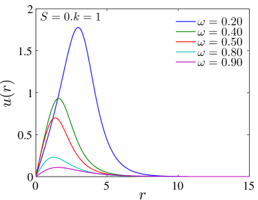
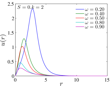
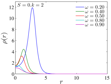
Figure 3: Radial profile of $S=0$ solitary waves in the 2D Soler model. Figures depict the first and second spinor components together with the solution density. Left (right) panels correspond to $k=1$ ($k=2$).

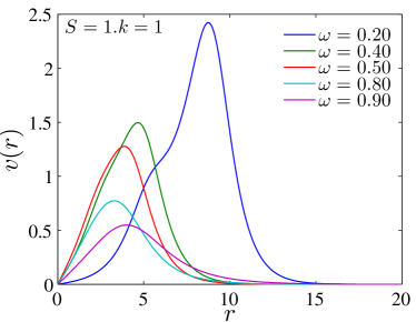
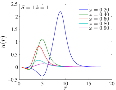
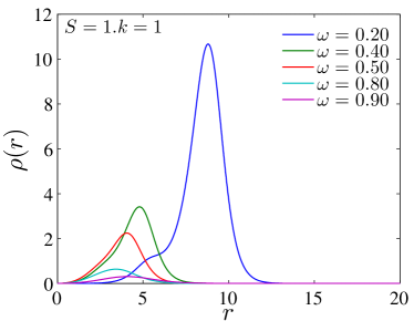
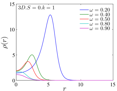
Figure 4: (Left panels) Radial profile of $S=1$ vortices in the cubic 2D Soler model. (Right panels) Radial profile of $S=0$ solitary waves in the cubic 3D Soler model. Figures depict the first and second spinor components together with the solution density.

Figure 5: Dependence of the charge of $S=0$ solitary waves in the 2D and 3D Soler models (left and right panels, respectively) with respect to the frequency for $1\leq k\leq 5$. Notice the existence of a minimum in the 2D (3D) curve for $k>1$ ($k\geq 1$), which will be related to stability changes (see Section 0.5).

4 Stability of solitary waves: theoretical results

In Section 2, we presented the equation governing the linear stability analysis of stationary solutions. In the present section, we will show the theoretical background related to spectral and orbital stability. Many of the results proposed herein will be numerically checked in Section 0.5.

4.1 Spectral stability of solitary waves

Prior to proceeding to the spectral stability analysis, we introduce some definitions.

The linearization of (3) at a solitary wave solution $\psi(t,x)=\phi_{\omega}(x)e^{-{i}\omega t}$ is represented by non-self-adjoint operators of the form

$$J(D_{m}-\omega+V(x,\omega)),\qquad\mbox{ with $J$ skew-adjoint, $J^{2}=-1$,}$$ (43)

where the matrix $J$ commutes with $D_{m}$ but not necessarily with the potential $V(x,\omega)$.

We say that the solitary wave is spectrally stable if the spectrum of its linearization operator has no points with positive real part. The spectral stability is the weakest type of stability; it does not necessarily lead to actual, dynamical one. The essential spectrum is easy to analyze: the application of Weyl’s theorem (see e.g. (cuevas-RS78, , Theorem XIII.14, Corollary 2) ) shows that the essential spectrum of the operator corresponding to the linearization at a solitary wave starts at $\pm(m-|{\omega}|){i}$ and extends to $\pm\infty{i}$. Thus, the spectral stability of the corresponding solitary wave would be a corollary of the absence of eigenvalues with positive real part in the spectrum of $J(D_{m}-\omega+V(\omega))$ in (43). The major difficulties in identifying the point spectrum $\sigma_{p}\big{(}J(D_{m}-\omega+V(\omega))\big{)}$ are due to the spectrum of $D_{m}$ extending to both $\pm\infty$; this prevents us from using standard tools developed in the NLS context.

In the absence of linear stability (that is when the linearized system is not dynamically stable), one expects to be able to prove orbital instability, in the sense of cuevas-GSS87 ; in cuevas-GO12 , such instability is proved in the context of the nonlinear Schrödinger equation; such results are still absent for the nonlinear Dirac equation.

Since the isolated eigenvalues depend continuously on the perturbation, it is convenient to trace the location of “unstable” eigenvalues (eigenvalues with positive real part) considering $\omega$ as a parameter. One wants to know how and when the “unstable” eigenvalues may emerge from the imaginary axis, particularly from the essential spectrum; that is, at which critical values of $\omega$ the solitary waves start developing an instability. Below, we describe the possible scenarios.

Instability scenario 1: collision of eigenvalues

picture(180,100)(-35,-50)

Birth of “unstable” eigenvalues out of collisions of imaginary eigenvalues. When the frequency $\omega$ of the solitary wave $\phi_{\omega}e^{-i\omega t}$ changes, the “unstable”, positive-real-part eigenvalues in the linearized equation could be born from the collisions of discrete imaginary eigenvalues The well-known Vakhitov–Kolokolov stability criterion cuevas-VK73 keeps track of the collision of purely imaginary eigenvalues at the origin and a subsequent birth of a positive and a negative eigenvalue. This criterion was discovered in the context of nonlinear Schrödinger equations, in relation to ground state solitary waves $\phi_{\omega}(x)e^{-{i}\omega t}$ (“ground state” in the sense that $\phi_{\omega}(x)$ is strictly positive; for more details, see cuevas-BL83 ). When $\partial_{\omega}Q(\omega)<0$, with $Q(\omega)=\|\phi_{\omega}\|_{L^{2}}^{2}$ being the charge of the solitary wave (2.2), then the linearization at a solitary wave has purely imaginary spectrum; when $\partial_{\omega}Q(\omega)>0$, there are two real (one positive, one negative) eigenvalues of the linearization operator. The vanishing of the quantity $\partial_{\omega}Q(\omega)$ at some value of $\omega$ indicates the moment of the collision of eigenvalues, when the Jordan block corresponding to the zero eigenvalue has a jump of two in its size. A nice feature of the linearization at a ground state solitary wave in the nonlinear Schrödinger equation is that its spectrum belongs to the imaginary axis, with some eigenvalues possibly located on the real axis; thus, the collision of eigenvalues at $\lambda=0$ is the only way the spectral instability could develop. In the NLD context, such a collision does not necessarily occur at $\lambda=0$; both situations as in Fig. 4.1 are possible. In cuevas-BCS15 , it was shown that in NLD (and similar fermionic systems) the collision of eigenvalues at the origin and a subsequent transition to instability is characterized not only by the Vakhitov–Kolokolov condition $dQ/d\omega=0$, but also by the condition $E(\omega)=0$, where $E$ is the value of the energy functional on the corresponding solitary wave.

Theorem 0.4.1

The algebraic multiplicity of the eigenvalue $\lambda=0$ of the linearization $\mathcal{A}_{\omega}$ at the solitary wave $\phi_{\omega}(x)e^{-{i}\omega t}$ has a jump of (at least) $2$ when at a particular value of $\omega$ either $\partial_{\omega}Q(\phi_{\omega})=0$ or $E(\phi_{\omega})=0$, with $Q(\phi_{\omega})$ and $E(\phi_{\omega})$ being the charge and the energy of the solitary wave $\phi_{\omega}(x)e^{-{i}\omega t}$.

The eigenvalues with positive real part could also be born from the collision of purely imaginary eigenvalues at some point in the spectral gap but away from the origin; we have recently observed this scenario in the cubic Soler model in two spatial dimensions cuevas-CKS+16a . Presently we do not have a criterion for such a collision of eigenvalues.

Instability scenario 2: bifurcations from the essential spectrum

The most peculiar feature of the linearization at a solitary wave in the NLD context is the possibility of bifurcations of eigenvalues with nonzero real part off the imaginary axis, out of the bulk of the essential spectrum.

picture(140,120)(-0,-60)

Possible bifurcations from the essential spectrum. Theoretically, when $|\omega|<m$, the nonzero-real-part eigenvalues could be born from the embedded thresholds at $\pm i(m+|\omega|)$, from the embedded eigenvalue in the bulk of the essential spectrum between the threshold and the embedded threshold, and from the collision of the thresholds at $\pm im$ when $\omega=0$. The article cuevas-BC16a gives a thorough analytical study of eigenvalues of the Dirac operators, focusing on whether and how such eigenvalues can bifurcate from the essential spectrum. Generalizing the Jensen–Kato approach cuevas-JK79 to the context of the Dirac operators, it was shown in (cuevas-BC16a, , Theorem 2.15) that for $|\omega|<m$ the bifurcations from the essential spectrum are only possible from embedded eigenvalues (Fig. 4.1, center), with the following exceptions: the bifurcation could start at the embedded thresholds located at $\pm{i}(m+|{\omega}|)$ (Fig. 4.1, left), or they could start at $\lambda=\pm im$ when $\omega=0$ (Fig. 4.1, right; this situation correspond to the collision of thresholds). Indeed, bifurcations from the embedded thresholds have been observed in a one-dimensional NLD-type model of coupled-mode equations cuevas-BPZ98 ; cuevas-CP06 . The bifurcations from the collision of thresholds at $\pm{i}m$ (when $\omega=0$) were demonstrated in cuevas-KS02 in the context of the perturbed massive Thirring model. One can use the Carleman–Berthier–Georgescu estimates cuevas-BG87 to prove that there are no embedded eigenvalues (hence no bifurcations) in the portion of the essential spectrum outside of the embedded thresholds cuevas-BC16a . As to the bifurcations from the embedded eigenvalues before the embedded thresholds, as in Fig. 4.1 (center), we do not have any such examples in the NLD context, although such examples could be produced for Dirac operators of the form (43) (with $V$ kept self-adjoint).

Instability scenario 3: bifurcations from the nonrelativistic limit

picture(140,120)(0,-70)

Bifurcations from $\lambda=0$ and hypothetical bifurcations from $\lambda=\pm 2m{i}$ in the nonrelativistic limit, $\omega\!\lesssim\!m$. The nonzero-real-part eigenvalues could be present in the spectrum of the linearization at a solitary wave $\phi_{\omega}e^{-i\omega t}$ for $\omega$ arbitrarily close to $m$; these eigenvalues would have to be located near $\lambda=0$ or near the embedded threshold at $\lambda=\pm 2mi$. The nonzero-real-part eigenvalues could be present in the spectrum of the linearization operators at small amplitude solitary waves for all $\omega\lesssim m$, being born “from the nonrelativistic limit”. It was proved in (cuevas-BC16a, , Theorem 2.19), under very mild assumptions, that the bifurcations of eigenvalues for $\omega$ departing from $\pm m$ are only possible from the thresholds $\lambda=0$ and $\lambda=\pm 2m{i}$; see Fig. 4.1. We now undertake a detailed study of these bifurcations; let us concentrate on the case $\lambda=0$. It is of no surprise that the behaviour of eigenvalues of the linearized operator near $\lambda=0$, in the nonrelativistic limit $\omega\lesssim m$, follows closely the pattern which one observes in the nonlinear Schrödinger equation with the same nonlinearity. In other words, if the linearizations of the nonlinear Dirac equation at solitary waves with $\omega\lesssim m$ admit a family of eigenvalues $\Lambda_{\omega}$ which continuously depends on $\omega$, such that $\Lambda_{\omega}\to 0$ as $\omega\to m$, then this family is merely a deformation of an eigenvalue family $\Lambda_{\omega}^{\mathrm{NLS}}$ of the linearization of the nonlinear Schrödinger equation with the same nonlinearity (linearized at corresponding solitary waves). To make this rigorous, one considers the spectral problem for the linearization at a solitary wave with $\omega\lesssim m$, applies the rescaling with respect to $m-\omega\ll 1$, and uses the reduction based on the Schur complement method, recovering in the nonrelativistic limit $\omega\to m$ the linearization of the nonlinear Schrödinger equation, and then applying the Rayleigh–Schrödinger perturbation theory; in cuevas-CGG14 , this approach was developed to prove the linear instability of small amplitude solitary waves $\phi_{\omega}(x)e^{-{i}\omega t}$ in the “charge-supercritical” NLD, in the nonrelativistic limit $\omega\lesssim m$.

Theorem 0.4.2

Assume that $f(s)=|s|^{k}$, where $k\in\mathbb{N}$ satisfies $k>2/n$ (and $k<2$ for $n=3$). Then there is $\omega_{1}<m$ such that the solitary wave solutions $\phi_{\omega}(x)e^{-{i}\omega t}$ (in the form of the Wakano Ansatz (2.5)) to NLD are linearly unstable for $\omega\in(\omega_{1},m)$. More precisely, let $\mathcal{A}_{\omega}$ be the linearization of the nonlinear Dirac equation at a solitary wave $\phi_{\omega}(x)e^{-{i}\omega t}$. Then for $\omega\in(\omega_{1},m)$ there are eigenvalues

$$\pm\lambda_{\omega}\in\sigma_{p}(\mathcal{A}_{\omega}),\qquad\lambda_{\omega}>0,\qquad\lambda_{\omega}=O(m-\omega).$$

Let us remark here that the restriction in the above theorem that $k$ is a natural number which was needed to make sure that the solitary wave family of the form of the Wakano Ansatz indeed exists. Theorem 0.4.2 extends to $f(s)=a|s|^{k}+O(|s|^{K})$, $a>0$, with $k\in(2/n,\,2/(n-2))$ ($k>2/n$ when $n\leq 3$) and $K>k$. The existence of the corresponding families of solitary waves was later proved in cuevas-BC16 . In that article, a general construction was given for small amplitude solitary waves in the nonlinear Dirac equation, deriving the asymptotics which we will need in the forthcoming stability analysis of such solitary waves. This is a general result proved for nonlinearities which are not necessarily smooth, thus applicable to e.g. critical and subcritical nonlinearities. We point out that the instability stated in Theorem 0.4.2 is in a formal agreement with the Vakhitov–Kolokolov stability criterion cuevas-VK73 ; one has $dQ(\omega)/d\omega>0$ for $\omega\lesssim m$. Conversely, we expect that the presence of eigenvalues with nonzero real part in the vicinity of $\lambda=0$ for $\omega\lesssim m$, is prohibited by the Vakhitov–Kolokolov stability criterion $\frac{dQ(\omega)}{d\omega}<0,$ $\omega\lesssim m.$ Similarly to how the NLS corresponds to the nonrelativistic limit of NLD, in the nonrelativistic limit of the Dirac–Maxwell system one arrives at the Choquard equation cuevas-Lieb77 ; see cuevas-CS12 and the references therein. The Choquard equation is known to be spectrally (in fact, even orbitally) stable cuevas-CL82 ; we expect that this implies absence of unstable eigenvalues bifurcating from the origin in the Dirac–Maxwell system. As we pointed out above, in the nonrelativistic limit $\omega\lesssim m$, there could be eigenvalue families of the linearization of the nonlinear Dirac operator bifurcating not only from the origin, but also from the embedded threshold (that is, such that $\lim_{\omega\to m}\Lambda_{i}(\omega)=\pm 2m{i}$). Rescaling and using the Schur complement approach shows that there could be at most $N/2$ such families bifurcating from each of $\pm 2m{i}$, with $N$ the number of components of a spinor field (in 3D Dirac, one takes $N=4$). Could these eigenvalues go off the imaginary axis into the complex plane? While for the nonlinear Dirac equations with a general nonlinearity the answer to this question is unknown, in the Soler model we can exclude this scenario. One can show that there are exact eigenvalues $\lambda_{\pm}(\omega)=\pm 2\omega{i}$, each being of multiplicity $N/2$; thus, we know exactly what happens to the eigenvalues which bifurcate from $\pm 2m{i}$, and expect no bifurcations of eigenvalues off the imaginary axis. The details are given in cuevas-BC17 .

Let us finish with a very important result: the existence of eigenvalues $\pm 2\omega{i}$ of the linearization at a solitary wave in the Soler model (3) is a consequence of having bi-frequency solitary wave solutions in the Soler model, in any dimension and for any nonlinearity. For more details, see cuevas-BC17 .

0.4.2 Orbital and asymptotic stability of solitary waves

The spectral analysis is one aspect of global analysis of the dynamical stability. In principle any spectral instability around a stationary solution should lead to a dynamical instability, namely the stationary solution is orbitally unstable. The contrapuntal statement that a stable stationary state has a spectrally stable linearized operator needs to be analyzed carefully. If the Dirac operator $D_{m}$ is perturbed by some zero-order external potential, the perturbation theory provides tools which allow one to analyze the linear stability of linearized operators of the form (43). Still some important restrictions on the potential appear (decay, regularity, and absence of resonances). Even if the perturbation analysis needs some work, it is much less involved compared to the complete spectral characterization of the linearized operator. This opens the gates to the analysis of the nonlinear stability. Prior to a bibliographical review of the available works in this direction, we make a remark. While in many models the orbital stability is obtained by using the energy as some kind of a Lyapunov functional, this is no longer possible for models of Dirac type since the energy is sign-indefinite. Even if there are some conserved quantities which allow one to control certain negative directions of the Hessian of the energy, the latter are in infinite number (“infinite Morse index”) and in most cases the conservation laws are not enough. The route “use linear stability to prove the asymptotic stability” seems to be the only one available for the sign-indefinite systems such as nonlinear Dirac, Dirac–Hartree–Fock, and others. As a result, due to the strong indefiniteness of the Dirac operator (the energy conservation does not lead to any bounds on the $H^{1/2}$-norm), we do not know how to prove the orbital stability cuevas-GSS87 but via proving the asymptotic stability first. The only exceptional case in nonlinear Dirac-type systems seems to be the completely integrable massive Thirring model in one spatial dimension cuevas-Thi58 , where additional conserved quantities arising from the complete integrability allow one to prove orbital stability of solitary waves cuevas-PS14 ; cuevas-CPS16 . Note that these conserved quantities are used not to control the negative directions but rather to construct a new Lyapunov functional. More precisely, by cuevas-PS14 , there is a functional $R$ defined on $H^{1}(\mathbb{R},\mathbb{C}^{2})$ (which contains terms dependent on powers of components of $\psi\in\mathbb{C}^{2}$ of order up to six) which is (formally) conserved for solutions to the massive Thirring model, and it is further shown that there is $\omega_{0}\in(0,m]$ such that for $\omega\in(-\omega_{0},\omega_{0})$ the solitary wave amplitude is a local minimizer of $R$ in $H^{1}$ under the charge and momentum conservation, and hence the corresponding solitary wave is orbitally stable in $H^{1}(\mathbb{R},\mathbb{C}^{2})$. Moreover, in cuevas-CPS16 , using the global existence of $L^{2}$-solutions for the (cubic) massive Thirring model cuevas-Can11 , the orbital stability of solitary waves in $L^{2}(\mathbb{R})$ has been shown, with the proof based on the auto-Bäcklund transformation. Now we turn to the asymptotic stability. In cuevas-CPS17 , the asymptotic stability was proved for the small energy perturbations to solitary waves in the Gross–Neveu model. The model is taken with particular pure-power nonlinearities when all the assumptions on the spectral and linear stability of solitary waves have been verified directly. This is, referring to the previous discussion, also the “proof of concept”: it is shown that there are translation-invariant systems based on the Dirac operator which are asymptotically stable; this is in spite of the energy functional being unbounded from below. First results on asymptotic stability were obtained in cuevas-Bou06 ; cuevas-Bou08 in the case $n=3$, in the external potential. There, the spectrum of the linear part of the equation $D_{m}+V$ is supposed to be, beside the essential spectrum $\mathbb{R}\setminus(-m,m)$, formed by two simple eigenvalues; let us denote them by $\lambda_{0}$ and $\lambda_{1}$, with $\lambda_{0}<\lambda_{1}$. From the associated eigenspaces, there is a bifurcation of small solitary waves for the nonlinear equation. The corresponding linearized operators are exponentially localized small perturbations of $D_{m}+V$, so that the perturbation theory allows a precise knowledge of the resulting spectral stability. Depending on the distance from $\lambda_{0}$ to $\lambda_{1}$ compared to the distance from $\lambda_{0}$ to the essential spectrum, the resulting point spectrum for the linearized operator may be discrete and purely imaginary and hence spectrally stable, or instead it may have nonzero-real-part eigenvalues if a “nonlinear Fermi Golden Rule” assumption is satisfied (similarly to the Schrödinger case, see cuevas-Sig93 ; cuevas-BP95 ; cuevas-SW99 ); in the latter case, linear and dynamical instabilities occur. In the former case, the linear stability follows from the spectral one via the perturbation theory. In any case, using the dispersive properties for perturbations of $D_{m}$, there is a stable manifold of real codimension $2$. Due to the presence of nonzero discrete modes, even in the linearly stable case, the dynamical stability is not guaranteed. Before considering the results on the dynamics outside this manifold, for perturbations along the remaining two real directions, one could ask what might happen if $D_{m}+V$ has only one eigenvalue. The answer follows quite immediately with the ideas from cuevas-Bou06 ; cuevas-Bou08 . In this case, there is only one family of solitary waves and it is asymptotically stable. Notice that the asymptotic profile is possibly another solitary wave but close to the perturbed one. In the one-dimensional case, this was studied properly in cuevas-PS14 . Note that the one-dimensional framework suffers from relatively weak dispersion which makes the analysis of the stabilization process more delicate. As for the dynamics outside the above-mentioned stable manifold, the techniques rely on the analysis of nonlinear resonances between discrete isolated modes and the essential spectrum where the dispersion takes place. This requires the normal form analysis in order to isolate the leading resonant interactions. The former is possible only if the “ nonlinear Fermi Golden Rule” is imposed. Such an analysis was done in cuevas-BC12 but in a slightly different framework: instead of considering the perturbative case the authors chose the translation-invariant case, imposing a series of assumptions that lead to the spectral stability of solitary waves. These assumptions are verified in some perturbative context with $V\neq 0$. This case is analyzed in cuevas-CT16 . The asymptotic stability approach from cuevas-PS14 ; cuevas-BC12 ; cuevas-CPS17 is developed under important restrictions on the types of admissible perturbations. These restrictions are needed to avoid the translation invariance and, most importantly, to prohibit the perturbations in the direction of exceptional eigenvalues $\pm 2\omega{i}$ of the linearization operator at a solitary wave $\phi_{\omega}(x)e^{-{i}\omega t}$. These eigenvalues are a feature of the Soler model (see cuevas-Gal77 ; cuevas-DR79 ); they are present in the spectrum for any nonlinearity $f$ in the Soler model (3), see cuevas-BC12a ; cuevas-Gal77 ; cuevas-DR79 . These eigenvalues are embedded into the essential spectrum when $|{\omega}|>m/3$ and violate the “nonlinear Fermi Golden Rule”: they do not “interact” (that is, do not resonate) with the essential spectrum; the energy from the corresponding modes does not disperse to infinity. This does not allow the standard approach to proving the asymptotic stability.

0.5 Stability of solitary waves: numerical results

Once the theoretical background on linear stability has been presented, we review in this section some very recent numerical results on this topic. To this aim, we first include a brief introduction to the Evans function formalism cuevas-Eva72 , and then, detailed results based on numerical analysis of BdG-like spectral stability are shown for both 1D and 2D Soler models. Let us recall some notation regarding the spectral stability, as we will make an extensive use of them in what follows. The essential spectrum corresponds to $\lambda\in{i}(-\infty,|\omega|-m]\cup{i}[-|\omega|+m,\infty)$. Embedded eigenvalues can be in the region $\lambda\in\pm{i}[-|\omega|+m,|\omega|+m]$ of the essential spectrum; for abbreviation, we denote this region as the embedded spectrum and the remaining part of the essential spectrum as non-embedded spectrum. In what follows, without lack of generality we will take $g=m=1$ unless stated otherwise.

0.5.1 Evans function approach to the analysis of spectral stability

The study of the spectral stability of the cubic 1D Soler model was performed in cuevas-BC12a , with the aid of the Evans function technique. This was the first definitive linear stability result (as well as the first definite stability result) in the context of the nonlinear Dirac equation. Let us give more details. In order to compute $\sigma\left(\mathcal{A}_{\omega}\right)$ we can employ the Evans function which provides an efficient tool to locate the point spectrum. The Evans function was first introduced by J.W. Evans cuevas-Eva72 ; cuevas-Eva72a ; cuevas-Eva72b ; cuevas-Eva75 in his study of the stability of nerve impulses. In his work, Evans defined $D(\lambda)$ to represent the determinant of eigenvalue problems associated with traveling waves of a class of nerve impulse models. $D(\lambda)$ was constructed to detect the intersections of the subspace of solutions decaying exponentially to the right and the subspace of solutions decaying exponentially to the left. Jones cuevas-Jon84 used Evans’ idea to study the stability of a singularly perturbed FitzHugh–Nagumo system. Jones called it the Evans function, and the notation $E(\lambda)$ is now common. The first general definition of the Evans function was given by Alexander et al. cuevas-AGJ90 in their study of the stability for traveling waves of a semi-linear parabolic system. Pego and Weinstein cuevas-PW92 expanded on Jones’ construction of Evans function to study the linear instability of solitary waves in the Korteweg–de Vries equation (KdV), the Benjamin–Bona–Mahoney equation (BBM), and the Boussinesq equation. Generally, the Evans function for a differential operator $\mathcal{D}$ is an analytic function such that $E(\lambda)=0$ if and only if $\lambda$ is an eigenvalue of $\mathcal{D}$, and the order of zero is equal to the algebraic multiplicity of the eigenvalue. Let us give a simple example which illustrates the nature of the Evans function. Consider the stationary Schrödinger equation

$$-\lambda^{2}u(x)=Hu(x),$$ (44)

where $H=-\partial_{x}^{2}+V$ with $V\in C(\mathbb{R})$, $\mathop{\mathrm{supp}}(V)\subset(-1,1)$. For $\lambda\in\mathbb{C}\setminus\{0\}$, $\mathrm{Re}(\lambda)>0$, it has the solutions $J_{+}(\lambda,x)$ and $J_{-}(\lambda,x)$, $x\in\mathbb{R}$, defined by their behaviour at $\pm\infty$:

$$J_{+}(\lambda,x)=e^{-\lambda x},\quad x\geq 1;\qquad\quad J_{-}(\lambda,x)=e^{+\lambda x},\quad x\leq-1.$$

We should note that $J_{+}$ and $J_{-}$ decay exponentially as $x\to\pm\infty$, respectively, and they have the same asymptotics at $\pm\infty$ as the solutions to the equation

$$-\lambda^{2}u(x)=H_{0}u(x),$$

where $H_{0}=-\partial_{x}^{2}$, which agrees with $H$ on $\mathbb{R}\setminus[-1,1]$. We call $J_{+}$ and $J_{-}$ the Jost solution to (44) and define the Evans function to be the Wronskian of $J_{+}$ and $J_{-}$:

$$E(\lambda)=W(J_{+},J_{-})(x,\lambda)=J_{+}(x,\lambda)\partial_{x}J_{-}(x,\lambda)-J_{-}(x,\lambda)\partial_{x}J_{+}(x,\lambda),$$

where the right-hand side depends only on $\lambda$. Vanishing of $E$ at some particular $\lambda\in\mathbb{C}$, $\mathrm{Re}(\lambda)<0$ shows that the Jost solutions $J_{+}$ and $J_{-}$ are linearly dependent, and there is $c\in\mathbb{C}\setminus\{0\}$ such that

$$\phi(x)=\begin{cases}J_{+}(x,\lambda),\qquad x\geq 0\\ cJ_{-}(x,\lambda),\qquad x<0\end{cases}$$

is $C^{1}$ and thus is an eigenfunction corresponding to an eigenvalue $\lambda^{2}$ of $H$. The construction for the one-dimensional Soler model is done by decomposing $L^{2}(\mathbb{R},\mathbb{C}^{4})$ into two invariant subspaces for the operator $\mathcal{A}_{\omega}$ introduced in (9): the “even” subspace, with even first and third components and with odd second and fourth components, and the “odd” subspace, with odd first and third components and with even second and fourth components; the direct sum of the “even” and “odd” subspaces coincides with $L^{2}(\mathbb{R},\mathbb{C}^{4})$. The Evans function corresponding to the “even” subspace is defined by

$$E_{even}(\lambda)=\mathop{\mathrm{det}}\left(R_{1},R_{3},J_{1},J_{2}\right),$$ (45)

where $R_{j}(x)$, $1\leq j\leq 4$, are the solutions to the equation $\lambda R=\mathcal{A}_{\omega}R$ with the initial data

$$R_{j}|_{x=0}=\mathbf{e}_{j},\qquad 1\leq j\leq 4,$$

where $\mathbf{e}_{j}$, $1\leq j\leq 4$, is the standard basis in $\mathbb{C}^{4}$. $J_{1}$ and $J_{2}$ are the Jost solution of $\mathcal{A}_{\omega}$, which are defined as the solutions to $\lambda\Psi=\mathcal{A}_{\omega}\Psi$ with the same asymptotics at $+\infty$ as the solutions to $\lambda\Psi=\mathbf{(}\mathbf{D}_{m}-\omega)\Psi$ which decay as $x\to+\infty$, where

$$\mathbf{D}_{m}=\begin{bmatrix}D_{m}&0\\ 0&D_{m}\end{bmatrix},\quad D_{m}=\begin{bmatrix}m&\partial_{x}\\ -\partial_{x}&-m\end{bmatrix}=-{i}(-\sigma_{2})\partial_{x}+m\sigma_{3}.$$

The Evans function corresponding to the “odd” subspace is constructed by using in (45) functions $R_{2}$ and $R_{4}$ instead of $R_{1}$ and $R_{3}$. We note that, by Liouville’s formula, the right-hand side in (45) does not depend on $x$. Fig. 6 shows the zeros of the Evans function which are plotted alongside with the essential spectrum for the linearization at the solitary waves in the 1D Soler model.

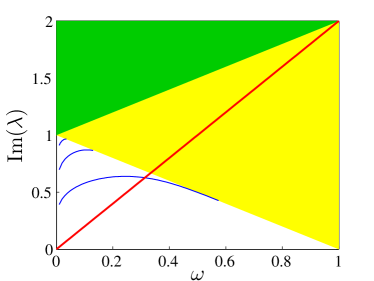
Figure 6: Eigenvalues corresponding to zeros of the Evans function in the upper half of the spectral gap as a function of $\omega$. Yellow area represents the part of the continuous spectrum that corresponds to ${i}L_{\pm}(\omega)$, while the green area represents the (doubly-covered) part of the continuous spectrum corresponding to both ${i}L_{\pm}(\omega)$ and $-{i}L_{\pm}(\omega)$. The eigenvalues $\lambda=2\omega i$ (red straight line) are embedded into the essential spectrum for $\omega>m/3$.

Later, in cuevas-CKS+16a , it was observed that the linearized operator admits invariant subspaces which correspond to spinorial spherical harmonics. This allows one to factorize the operator, essentially reducing the consideration to a one-dimensional setting, and to perform a complete numerical analysis of the linearized stability in the nonlinear Dirac equation in two spatial dimensions and give partial results in three dimensions, basing our approach on both the Evans function technique and the linear stability analysis using spectral methods. For the two-dimensional Soler model, we can use the same process as the one-dimensional case to construct the Evans function. Recall (see (29)) that $\mathcal{A}_{\omega}$ acts invariantly on $\mathcal{X}_{q}$ for each $q\in\mathbb{Z}$ and $\mathcal{A}_{\omega,q}=\mathcal{A}_{\omega}|_{\mathcal{X}_{q}}$. We consider the case $S=0$. The Evans function for each $\mathcal{A}_{\omega,q}$ is defined by

$$E_{q}(\lambda)=\mathop{\mathrm{det}}(R^{+}_{q},R^{-}_{q},Y_{1},Y_{2}).$$

Here $R^{+}_{q}$ and $R^{-}_{q}$ are linearly independent solutions to the equation $\lambda R=\mathcal{A}_{\omega,q}R$ with the following linearly independent initial data at $r=0$

$$\begin{bmatrix}-\lambda-(\omega+f_{0})\frac{{i}q}{|q|}\\ 0\\ {i}|q|\\ q\end{bmatrix}\quad\text{and}\quad\begin{bmatrix}0\\ -{i}\lambda\frac{q}{|q|}+\omega+f_{0}\\ |q|\\ {i}q\end{bmatrix},$$

where $f_{0}=m-g\left(u^{2}(0)-v^{2}(0)\right)$. The Jost solutions $Y_{1}$ and $Y_{2}$ of $\mathcal{A}_{\omega,q}$ are defined as the solution to $\lambda Y=\mathcal{A}_{\omega,q}Y$ with the same asymptotics at $+\infty$ as the solutions to $\lambda Y=\mathbf{D}_{q}Y$ where

$$\mathbf{D}_{q}=\left[\begin{array}[]{cc}-\sigma_{1}\frac{{i}q}{r}&{D}_{m}-\omega I_{2}\\[8.61108pt] -{D}_{m}+\omega I_{2}&-\sigma_{1}\frac{{i}q}{r}\end{array}\right],\qquad q\in\mathbb{Z}.$$

0.5.2 Bogoliubov–de Gennes analysis: The one-dimensional case

Let us recall from the analysis shown in Section 4 that near the non-relativistic limit ($\omega\lesssim m$), the stability of solitary waves formally agrees with the Vakhitov–Kolokolov stability criterion $\partial_{\omega}Q(\phi_{\omega})<0$ cuevas-VK73 . In particular, there is no positive eigenvalue emerging from $\lambda=0$ for $\omega\lesssim m$ as long as $k\leq 2$ (and, consequently, the solitary waves are spectrally stable), while in the case $k>2$ there is a pair of (a positive and a negative) eigenvalues which result in linear instability. As it turns out, in the one-dimensional case, the Vakhitov–Kolokolov stability criterion agrees with the observed stability of solitary waves not only in the nonrelativistic limit, but for all frequencies $\omega\in(0,m)$, as our numerical calculations show below. Evans function analysis presented above also shows that solitary waves do not present oscillatory instabilities (i.e. there are no complex $\lambda$’s with nonzero real part) in the 1D case; the instability could only develop when eigenvalues collide and bifurcate from the origin. Additionally, for any $k$, the existence of an eigenvalue $\lambda=\pm 2\omega{i}$ is a consequence of the $\mathbf{SU}(1,1)$-invariance of the Soler model cuevas-Gal77 ; cuevas-DR79 . This mode, which does not give rise to any instability, is embedded into the essential spectrum for $\omega\in(m/3,m)$ (see Fig.7). Let us mention that it was shown in cuevas-MQC+12 ; cuevas-SQM+14 that attempts to apply Derrick’s argument cuevas-Der64 to stability of solitary waves in the context of the nonlinear Dirac equation cuevas-Bog79 ; cuevas-SV86 – in particular, the so-called Bogolubsky criterion – do not seem to work. This is not particularly surprising, given that Derrick’s empirical argument, based on singling out one family of perturbations of a solitary wave and checking whether the solitary wave corresponds to the energy minimum on this curve, was introduced in the context of the second order systems, appealing to our Newtonian-world intuition. Apparently, this approach does not necessarily work in the context of the first order systems, such as the Dirac equation. Another surprising result was explored by some of the present authors in cuevas-CKS15 . It corresponds to the BdG analysis using finite difference discretization of the 1D Soler model; that is, the spatial derivatives $\partial_{x}f(x)$ in (7) are substituted by the central difference $(f_{n+1}-f_{n-1})/(2h)$. This method is tantamount to using the collocation points of (38) and (40) with $N$ collocation points, a domain $x\in[-L,L]$ and $h=2L/N$. Fig. 7 shows the stability eigenvalues for $k=1$ and $L=80$ with a discretization step $h=0.1$. Although there are instabilities caused by eigenvalue collisions in the non-embedded spectrum, we neglected them, as they disappear in the limit of $h\rightarrow 0$ and $L\rightarrow\infty$. The solitary waves were found to be unstable for small $\omega$, with a growth rate that decreases when $\omega$ is increased. The source of instabilities is a localized mode (with non-zero real part of its eigenvalue even when $\omega\rightarrow 0$) that enters the essential spectrum at $\omega\approx 0.037$ i.e. it embeds into the essential spectrum. Once inside the linear modes band, this localized mode causes multiple “bubbles”, but at $\omega\approx 0.632$, it returns to the imaginary eigenvalue axis and the solitary wave becomes stable. Nevertheless, this stability is ephemeral, as the solitary waves become unstable again at $\omega\approx 0.634$. From this point, there is a succession of instability bubbles, whose amplitude (i.e., the maximal growth rate associated with them) decreases with $\omega$. In order to observe the behavior of bubbles when the domain is enlarged, the same figure compares the growth rates for $L=40$, $100$ and $150$. It is observed that the number of bubbles increases with $L$, but their width decreases. In any case, the envelope of the bubbles tends to zero asymptotically when $\omega$ approaches 1, in a similar way as it was observed for dark solitons in the discrete nonlinear Schrödinger equation (DNLS) setting cuevas-JK99 . The convex nature of the relevant (apparent) envelope curve is inconclusive in connection with the stability aspect; it is unclear, based on those computations, whether the curve, as $h\rightarrow 0$, still intersects the axis and no longer features an unstable mode past a critical value of $\omega$. The alternative scenario is that the approach to the stable NLS limit of $\omega\rightarrow 1$ is merely asymptotic.

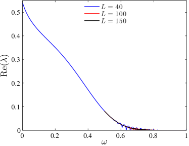
Figure 7: Spectrum of the stability matrix (10) for solitary waves in domain $[-L,L]$ with $L=40$ obtained using finite differences with $N=800$ grid points in the cubic ($k=1$) case. For the sake of simplicity, only the positive real and imaginary parts of the eigenvalues are shown. Dots correspond to Evans function predictions. Right panel displays only the maximum values of $\mathrm{Re}(\lambda)$ (i.e. the growth rates) and includes the values for $L=40$, $L=100$, and $L=150$.

In order to find out a strategy which assures a spectral accuracy of BdG stability analysis which is also correlated to the Evans’ function analysis, we used spectral collocation methods in cuevas-CKS+15 . We utilized two case examples of such methods therein: the Fourier Spectral Collocation Method, which implicitly enforces periodic boundary conditions, and the Chebyshev Spectral Collocation Method, which enforces (homogeneous) Dirichlet boundary conditions (see Subsection 3.2). The advantage of the Finite Difference Method with respect to the other ones concerns the fact that the resulting stability matrix is sparse. In the computations performed in that work and that will be presented below, $N=800$ collocation points were taken in a domain $[-L,L]$, with a discretization parameter $h=1/(2L)$; this value coincides with the distance between grid points in the Fourier collocation and finite difference methods, but not in the Chebyshev collocation as the grid points are not equidistant. Increasing the node numbers to $N=1200$ does not seem to qualitatively improve the findings. In Fig. 8 we examine the dependence of the imaginary part of the eigenvalues $\lambda$ with respect to the frequency $\omega$ of the solution for both spectral methods in the cubic case of $k=1$. In addition to the $\lambda=\pm 2\omega{i}$ mode, the different methods have additional modes which can be compared also with the Evans function analysis outcome of Fig. 6. We thus find that the comparison of the Fourier spectral collocation method with the Evans function analysis (Fig. 6) seems qualitatively (and even quantitatively) to yield very good agreement with the exception of a mode that seems to initially grow steeply (for small $\omega$) and subsequently to slowly asymptote to the band edge (as $\omega$ increases). This mode is shown in the right panel of Fig. 9, while the left panel of the figure illustrates a prototypical example of the Fourier spectral collocation method spectrum for $\omega=0.1$. From the above panel, we can immediately infer that this mode is, in fact, spurious and an outcome of the discretization as it carries a staggered profile that cannot be supported in the continuum limit. In the left panel of the same figure, we can see the existence of additional spurious modes forming bubbles of complex eigenvalues. However, the fact that these bubbles are occurring at the eigenvalues of the continuous spectrum assures us that these are spurious instabilities due to the finite size of the domain and ones which disappear in the $L\rightarrow\infty$, $h\rightarrow 0$ limit. This is confirmed by Fig. 10 which shows that as we decrease $h$ (and increase the number of lattice sites, approaching the continuum limit for a given domain size) the growth rate of such spuriously unstable eigenmodes accordingly decreases.

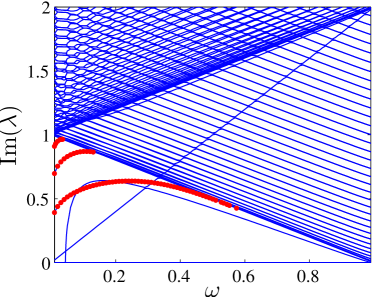
Figure 8: Imaginary part of the spectrum of the stability matrix (10) for solitary waves in domain $[-L,L]$ with $L=40$ obtained using Fourier (left) and Chebyshev (right) spectral collocation method with $N=800$ grid points in the cubic ($k=1$) case. For the sake of simplicity, only the positive imaginary parts of the eigenvalues are shown. Dots correspond to Evans function predictions.

Figure 9: Spectral plane of a solitary wave with $\omega=0.1$ (cubic case, $L=40$, and $N=800$) obtained using the Fourier spectral collocation method (left panel). The typical profile of two modes corresponding to spurious eigenvalues is depicted in the right panel. In particular, we have included the mode with $\mathrm{Re}(\lambda)=0$ which does not arise in the Evans’ function analysis of Subsection 0.5.1 together with the largest real part eigenvalue, which is also spurious.

Figure 10: Growth rates (i.e. maximum of the real part of the eigenvalues) for a solitary wave with $L=40$ in the cubic case using the Fourier spectral collocation method. The number of grid points is either $N=800$ or $N=200$.

Remarkably, the finite difference spectrum of Fig. 7 is the one that seems most “distant” from the findings of the Evans function method. While all four of the internal modes of the latter spectrum seem to be captured by the finite difference method, three additional modes create a nontrivial disparity. Two of them are in fact “benign” and maintain an eigenvalue below the band edge of the continuous spectrum for all values of $\omega\in(0,m)$. However, as explained in cuevas-CKS15 , we also observe the existence of an eigenmode embedded in the essential spectrum. Unfortunately, this mode is accompanied by a real part in the corresponding eigenvalue and hence gives rise to a spurious instability. While the origin of this mode starting from the so-called anti-continuum limit will be thoroughly explained in Section 0.7, the persistence and especially the instability inducing nature of such a mode remains an open problem as the continuum limit is approached. Fig. 11 presents a graph analogous to Fig. 9 but for the finite difference method. The undesirable unstable mode, as well as additional spurious modes are explicitly indicated through the eigenvector profiles of the right panel.

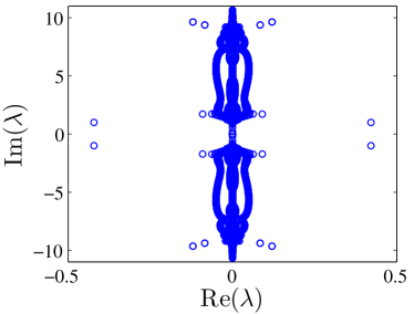
Figure 11: Spectral plane of a solitary wave with $\omega=0.1$, $L=40$ and $N=800$ in the cubic case, using finite difference discretization (left panel). The typical profile of three modes corresponding to spurious eigenvalues is depicted in the right panel. In particular, we have included the two modes with $\mathrm{Re}(\lambda)=0$ which do not arise in the Evans function analysis together with the embedded spurious mode.

The scenario of the Chebyshev spectral collocation method bears advantages and disadvantages in its own right. Although it gives an accurate result for the imaginary part of the eigenvalues, their real part grows for large $\mathrm{Im}(\lambda)$, as is also shown in Fig. 12. Additionally, as indicated in cuevas-Boy01 , approximately half of the values of the spectrum are spurious within the Chebyshev collocation methods, so they should be excluded from consideration. Furthermore, one can observe that in this case as well, spurious instability bubbles arise (see the right panel of Fig. 12), yet we have checked that these disappear in the continuum limit of $h\rightarrow 0$.

Figure 12: Spectral plane of a solitary wave with $\omega=0.4$, $L=40$, and $N=800$ in the cubic case, using the Chebyshev spectral collocation method. The right panel is a zoom of that on the left, illustrating the weak, spurious instabilities (which disappear as the continuum limit is approached).

As a final aspect of the spectral considerations that we provide herein, we have examined the instability that arises e.g. from the Chebyshev spectral collocation method for larger values of $k$. Recall that the Chebyshev spectral collocation method predicts (at least as regards the point spectrum out of the non-embedded spectrum) that there is no instability for any $\omega$ in the case of $k=1$, in agreement with the Evans function analysis and cuevas-PS16 . The method identifies an instability for such point spectrum eigenvalues only for $k>2$. The relevant instability predicted numerically in the $k$-$\omega$ plane is illustrated in Fig. 13. We note that this instability is precisely captured by the Vakhitov–Kolokolov criterion, i.e. it precisely corresponds to the condition $\partial_{\omega}Q(\omega)=0$, in agreement with cuevas-BCS15 . Hence, by analogy with the nonrelativistic limit $\omega\rightarrow m=1$, we expect this to be an instability associated with the collapse of the latter model (however, we will observe a key dynamical difference, in comparison to the NLS, in Section 0.6). Nevertheless, it is relevant to point out here that the NLD, contrary to the NLS, does not exhibit an instability for all $\omega$ when $k>2$. The instability is instead limited to $\omega>\omega_{c}(k)$, as characterized by the curve of Fig. 13. Hence, it can be inferred that the instability is mitigated by the relativistic limit of the NLD and only occurs in an interval of frequency values including the non-relativistic limit $\omega\rightarrow m=1$, yet not encompassing the full range of available frequencies in the relativistic case.

Figure 13: Exponential bifurcation loci in the $\omega_{c}$-$k$ plane for the 1D Soler model. The solitary waves under the curve are linearly (spectrally) stable, while the ones above the curve are linearly unstable. Full line corresponds to the application of the Vakhitov–Kolokolov criterion (i.e. points for which $\partial_{\omega}Q(\omega)=0$), whereas the dots correspond to the stability calculations.

0.5.3 Bogoliubov–de Gennes analysis: The two- and three- dimensional cases

From the experience acquired with the study of the stability of solitary waves in one spatial dimension, it is clear that a Chebyshev spectral collocation method must be followed in order to analyze the stability in higher-dimensional solitary waves. This is the approach followed in the present section, which summarizes the results of cuevas-CKS+16a . Let us remember that the spectrum of $\mathcal{A}_{\omega}$ is the union of spectra of the one-dimensional spectral problems (29): $\sigma\left(\mathcal{A}_{\omega}\right)=\mathop{\cup}_{q\in\mathbb{Z}}\sigma\left(\mathcal{A}_{\omega,q}\right)$. In our numerics we have analyzed values of $q\in[-6,6]$, although the main phenomenology is captured by $|q|\leq 4$ and those are the values shown in the next figures for the sake of better visualization.

Figure 14: Dependence of the (left) imaginary and (right) real part of the eigenvalues with respect to the frequency $\omega$ of solitary waves in the 2D Soler model with cubic ($k=1$) nonlinearity. Top (respectively, bottom) panels correspond to $S=0$ solitary waves ($S=1$ vortices). For the sake of clarity, we only included the values $|q|\leq 4$. Full (dashed) lines in left panels represent the eigenvalues for $q\geq 0$ ($q<0$). The correspondence between colors and $|q|$ is indicated in the legend of right panels.

We start by considering the stability of $S=0$ solitary waves in the cubic ($k=1$) case. Top panels of Fig. 14 show the dependence of the real and imaginary parts of the eigenvalues with respect to the stationary solution frequency $\omega$. From the spectral dependencies we can deduce several features of the 2D Soler model. First of all, it is known that the 2D NLS is charge-critical, and the zero eigenvalues are degenerate cuevas-SS99 : they have higher algebraic multiplicity. In the NLD case, however, this degeneracy is resolved: in the $S=0$ case, as $\omega$ starts decreasing, two eigenvalues (corresponding to $q=0$) start at the origin when $\omega=1$ and move out of the origin for $\omega\lesssim 1$. The absence of the algebraic degeneracy of the zero eigenvalue prevents solitary waves from NLS-like self-similar blow-up which is possible in the charge-critical NLS cuevas-Mer90 . Secondly, the $\mathbf{U}(1)$ symmetry and the translation symmetry of the model result in zero eigenvalues with $q=0$ and $|q|=1$, respectively (in both $S=0$ and $S=1$ cases). Thirdly, as in the 1D Soler model, the eigenvalues $\lambda=\pm 2\omega{i}$, which are associated with the $\mathbf{SU}(1,1)$ symmetry of the model, are also present. This eigenvalue pair corresponds to $q=\mp 1$, i.e., to an excited linearization eigenstate. Finally, contrary to the 1D case, where the solitary waves corresponding to any $\omega<1$ are spectrally stable, the $S=0$ solitary wave is linearly unstable for $\omega<0.121$ because of the emergence of nonzero-real-part eigenvalues via a Hamiltonian Hopf bifurcation in the $|q|=2$ spectrum at $\omega=0.121$. Another Hopf bifurcation occurs corresponding to $|q|=3$ (at $\omega=0.0885$), then yet another one corresponding to $|q|=4$ for lower $\omega$. Vortices with $S>0$ are unstable for every $\omega$, because of the presence in the spectrum of quadruplets of complex eigenvalues. These quadruplets emerge (and disappear) for different values of $q$ via direct (inverse) Hopf bifurcations (see bottom panels of Fig. 14). The spectrum for $S\geq 2$ vortex is quite similar to that of $S=1$; for this reason, we do not analyze it further. Notice that the eigenvalues $\lambda=\pm 2\omega i$ generally correspond to the particular mode with $q=\mp(2S+1)$.

Figure 15: Dependence of the (left) imaginary and (right) real part of the eigenvalues with respect to the frequency $\omega$ of $S=0$ solitary waves in the 2D Soler model with quintic ($k=2$) nonlinearity. For the sake of clarity, we only included the values $|q|\leq 4$. Full (dashed) lines in the left panel represent the eigenvalues for $q\geq 0$ ($q<0$). The correspondence between colors and $|q|$ is indicated in the legend of the right panel.

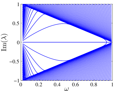
Figure 16: Dependence with respect to $\omega$ of the (left) imaginary and (right) real part of the eigenvalues of the one-dimensional invariant ($q=0$) subspace of $S=0$ solitary waves in the 3D Soler model with cubic ($k=1$) nonlinearity.

Figure 17: Critical frequency for radially-symmetric ($q=0$) exponential bifurcations in the 2D and 3D Soler model, as a function of the exponent $k$. For $(\omega_{c},1)$, the $S=0$ solitary waves are linearly unstable. For $k\leq 2/n$, with $n$ being the system dimension, there is no linear instability for $\omega\lesssim 1$, according to the Vakhitov–Kolokolov criterion (see Section 4).

It is especially interesting that a wide parametric (over frequencies) interval of stability of solitary waves with $S=0$ can also be observed in the quintic ($k=2$) NLD case (see Fig. 15); while the quintic NLS solitary waves blow up (even in one dimension), the quintic NLD solitary waves are stable even in two dimensions, except for the interval $\omega<0.312$ where the coherent structures experience the same Hopf bifurcation as in the cubic case, and for $\omega>0.890$ where an exponential instability created by radial $q=0$ perturbations emerges. This exponential instability is predicted by the Vakhitov–Kolokolov criterion as it coincides with the point at which $\partial_{\omega}Q(\omega)=0$ (see Fig. 5). Perhaps even more remarkably, Fig. 16 illustrates that this stability of NLD solitary waves against radial perturbations can be found in suitable frequency intervals even in 3D cuevas-CGG14 . Both of the above cases (quintic 2D and cubic 3D Soler models) are charge-supercritical i.e., the charge goes to infinity in the nonrelativistic limit $\omega\to 1$. Contrary to the pure-power supercritical NLS whose solitary waves remain linearly unstable for all frequencies, solitary waves in the Soler model become spectrally stable when $\omega$ drops below some dimension-dependent critical value $\omega_{c}=\omega_{c}(n,k)$, with $n$ being the number of spatial dimensions. Fig. 17 shows those critical frequencies (associated with $q=0$ and radially-symmetric collapse) as a function of the nonlinearity parameter $k$ for $n=2$ and $n=3$. For $\omega\in(\omega_{c},1)$, the NLD solitary waves are linearly unstable. Below $\omega_{c}$ the linear instability disappears. For $k\leq 2/n$, there is no linear instability for $\omega\lesssim 1$. In the particular case of cubic ($k=1$) 3D Soler model, we have that $\omega_{c}\approx 0.936$. This value was identified by Soler in his original paper cuevas-Sol70 as the value at which both the energy and charge of solitary waves have a minimum. Hence, we indeed find that the radially-symmetric collapse-related instability ceases to be present below this critical point.

0.6 Dynamics

Once the stability properties of solitary waves and vortices of the Soler model have been elucidated, it is now natural to turn our attention towards the observation of their dynamical properties. In the one-dimensional case, we will analyze some integration schemes in order to observe their suitability for simulation of solitary waves in nonlinear Dirac equations. In addition, the dynamics of unstable solutions in equations with high-order instabilities (i.e. $k>1$) will be shown. Finally, the dynamics of unstable solitary waves and vortices for the 2D Soler model will be considered.

0.6.1 One-dimensional solutions

This subsection is divided into two parts. In the first one, we will show the evolution of stable solitary waves within several numerical integrators in the cubic ($k=1$) Soler model. The second part deals with the evolution of unstable solitary waves with $k>1$. Most of the results presented herein are taken from cuevas-CKS+15 .

Stable solutions

We turn here our attention to the implications of spectral collocation methods to the nonlinear dynamical evolution problem. We focus on the case of $k=1$. Given the large (yet spurious) growth rate of the modes emerging from the Chebyshev spectral collocation method and the spurious point spectrum instability of the finite difference method, for our dynamical considerations, we will focus our attention to the Fourier spectral collocation method results. As discussed in Subsection 0.5.2, in that method too, there exist spurious modes which, as expected, are found to affect the corresponding dynamics. As a dynamical outcome of these modes, the solitary waves are found to be destroyed after a suitably long evolution time, although the time for this feature is controllably longer in comparison to the one observed in cuevas-SQM+14 . This, in turn, suggests the expected stability of the solitary wave solutions, in accordance with what was proposed in Section 0.5. As a prototypical diagnostic of the dynamical stability of solitary waves in a finite domain $[-L,L]$, we have monitored the $L^{2}$-error in a similar fashion as in cuevas-SQM+14 :

$$\varepsilon_{2}(t)=\Big{(}\int\ \left|\rho(t,x)-\rho(0,x)\right|^{2}\,dx\Big{)}^{1/2},$$

with $\rho=\psi^{\ast}\psi$ being the charge density. A first approach to the dynamics problem is accomplished by choosing a fixed-step 4th order Runge–Kutta method. We observe that the lifetime is longer when the frequency $\omega$ is fixed and the domain length $L$ is increased. This is associated with the decrease of the size of spurious instability bubbles, as we approach the infinite domain limit. A similar decrease of the growth rate is observed for a given $L$, when the discretization spacing $h$ is decreased (i.e., as the continuum limit is approached), in accordance with the spectral picture of Fig. 10. In addition, if $L$ is fixed, the lifetime is longer when $\omega$ is increased. This is summarized in Fig. 18. This is, of course, in consonance with earlier observations such as those of cuevas-SQM+14 , however, our ability to expand upon the lifetimes as the domain and discretization parameters are suitably tuned suggests that in the infinite domain, continuum limit such instabilities could be made to disappear upon suitable selection of the numerical scheme. As a final comment, we note that the growth rates observed in Fig. 18 are consonant with the maximal (yet spurious) instability growth identified in Fig. 10. This is yet another indication that this growth featured in the time dynamics is a spurious by-product of the discretization scheme, rather than a true feature of the corresponding continuum problem.

Figure 18: Stable solitary waves simulations in cubic 1D Soler model using a 4th-order Runge–Kutta integrator with a Fourier spectral collocation method. The norm error is compared for different domain sizes and frequencies. In every case, the time step of the integrator is $\Delta t=0.05$.

Table 1: Comparison between the critical times for which $\varepsilon_{2}>10^{-3}$ using the Fourier Spectral Collocation method with a 4th-order Runge–Kutta integrator ($t_{1}$) and the Operator Splitting Method of cuevas-SQM+14 ($t_{2}$).

	$\omega=0.1$		$\omega=0.5$
$L$	$t_{1}$	$t_{2}$	$t_{1}$	$t_{2}$
50	1220	121	5620	6614
75	1320	122	8480	8724
100	1990	122	14660	9937
125	2540	120	14660	11670
150	3120	122	14660	13560

In Table 0.6.1 we compare the critical time for which $\varepsilon_{2}>10^{-3}$ within the Fourier spectral collocation method and the corresponding time for the 4th order operator splitting algorithm used in cuevas-SQM+14 for which we have the frequencies $\omega=0.1$ and $\omega=0.5$ and different domain lengths $L$. As can be seen from the comparison, although in some cases (e.g. for $\omega=0.5$ and $L=50$) the observed destabilization may happen later for the scheme of cuevas-SQM+14 , generally the Fourier spectral collocation method code explored herein allows to enhance the wave lifetime, in some cases by an order of magnitude. This can be further improved by tweaking parameters such as $h$ and the time spacing of the integrator $\Delta t$, as discussed above. Hence, our conclusion is that despite the artificial instabilities existing in the spectral picture and their dynamical manifestation, it is anticipated that the continuum, real line variant of the problem is spectrally stable for all $\omega\in(0,m)$ in the case of $k=1$. A tweak to the problem could be, on the one hand, to use adaptive step-size integrators cuevas-HNW93 . The case of 4th-5th order Dormand–Prince integrator cuevas-DP80 does not improve significantly the solitary wave lifetime. On the other hand, when using a 2nd-3rd order Runge–Kutta integrator supplemented by a TR-BDF2 scheme (i.e. a trapezoidal rule step as a first stage and a backward differentiation formula as a second stage) cuevas-SH96 , many of the spurious eigenvalues can be damped out and the lifetimes are strongly enhanced.

Unstable solutions for high-order nonlinearity

Having observed that the solitary wave solutions of the problem with $k=1$ (and, in fact, with any $k<2$) are dynamically stable, we now turn our attention to the dynamics associated with the instability in the case $k>2$, for $\omega>\omega_{c}(k)$, as per Fig. 13. Figure 19 shows the evolution of an exponentially unstable solitary wave with $k=3$ and $\omega=0.9$. We can observe the existence of oscillations around a stable fixed point. This fixed point approximately corresponds to the solitary wave with frequency $\omega\approx 0.82$, for which the solution is spectrally stable. This is in stark contrast with the supercritical dynamics of the Nonlinear Schrödinger equation. There, the instability directly leads to collapse and an indefinite growth of the amplitude of the solution. On the contrary, in the case of the Soler model, for any value of $k$ for which the solution may become unstable, there exists (for the same $k$) an interval of spectrally stable states of the same type. Hence, the solution to the Soler model does not escape towards collapse but rather departs from the vicinity of the unstable fixed point solution and finds itself orbiting around a center, i.e., a stable solitary wave structure.

Figure 19: (Left) Time evolution of a 1D solitary wave with nonlinearity exponent $k=3$ and frequency $\omega=3$. (Right) Spectral plane of the solitary wave whose evolution in traced in the left panel.

0.6.2 Two-dimensional solutions

This subsection reviews the results on the dynamics of 2D solitary waves and vortices shown in cuevas-CKS+16a . In order to simulate their dynamics, Chebyshev spectral methods and finite difference methods are not the most suitable ones, because of the presence of many spurious eigenvalues, and the dimensionality of the problem makes the TR-BDF2 schemes difficult to implement because of the high memory requirements. Thus, it seems that the optimal way to proceed is to use a Fourier spectral collocation method, which, as shown for the 1D problem, works fairly well as long as the frequency $\omega$ is not close to zero. Consequently, periodic boundary conditions must be supplied to our problem. This is less straightforward when working in polar coordinates in the domain $(0,L)\times[0,2\pi)$. For this reason, we opt to work with a purely 2D problem in rectangular coordinates in the domain $(-L,L]\times(-L,L]$. The simulations we show below have been performed with a Dormand–Prince numerical integrator using such a spectral collocation scheme with the aid of Fast Fourier Transforms (39).

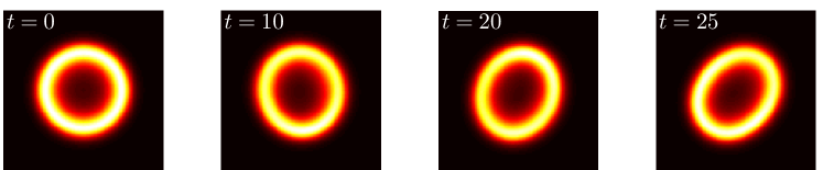
Figure 20: Snapshots showing the evolution of the density of an unstable $S=0$ solitary wave with $\omega=0.12$ in the cubic 2D Soler model. The solitary wave which initially had a circular shape becomes elliptical and rotates around the center of the original solitary wave.

Figure 21: Spectral planes of the unstable solitary waves whose dynamics are depicted in Figs. 20 and 22 (left and right panels, respectively). Each color represents a different value of $q$ as in Fig. 14.

Figure 22: Snapshots showing the evolution of the density of an unstable $S=1$ vortex with $\omega=0.6$ in the cubic 2D Soler model.

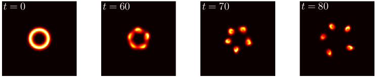
Figure 23: Snapshots showing the evolution of the density of an unstable $S=2$ vortex with $\omega=0.6$ in the cubic 2D Soler model.

A prototypical example of the evolution of unstable $S=0$ solitary waves for $k=1$ is shown in Fig. 20. As can be observed, the radial symmetry in the density of $S=0$ solitary waves is spontaneously broken and, as a result, the coherent structures become elliptical and rotate around the center of the circular density of the original solitary wave in line with the expected amplification of the $q=2$ unstable eigenmode (see spectrum at the left panel of Fig. 21). The dynamical outcome of $S=1$ vortices for $k=1$ is shown in Fig. 22, whose instability (see spectral plane at right panel of Fig. 21) leads to the splitting into three smaller ones; in particular, the first spinor component splits into structures without angular dependence, whereas the second component splits into corresponding ones with angular dependence $\propto e^{i\theta}$, in accordance with the Ansatz of Eq. (19). This preserves the total vorticity across the two components. The instability of an $S=2$ vortex eventually leads to the emergence of five similar structures to the previous case, again preserving the total vorticity (see Fig. 23).

[width=.5]cuevas-fig27

Figure 24: Isosurface for the density of the $S=0$ solitary wave in the quintic 2D Soler model with $\omega=0.94$.

Finally, we have analyzed the outcome of the instabilities caused by radially-symmetric perturbations in the $k=2$ case for $\omega>\omega_{c}$ (see Fig. 24). We can observe the typical behavior of such solutions, i.e. the density width (and amplitude) oscillate leading to a “breathing” structure, but there is no collapse. This phenomenology is reminiscent of the 1D case of the previous subsection (as in Fig. 19).

0.7 The (one-dimensional) Discrete Nonlinear Dirac equation

In the present section, we will take a somewhat different path from the previous ones. In particular, we will consider the existence, stability, and dynamics of solitary waves in a discrete version of the 1D Soler model. This equation is simply obtained, as explained in Subsection 0.5.2, by substituting the spatial derivatives $\partial_{x}\psi(t,x)$ in (7) by the central difference $\epsilon(\psi_{n+1}(t)-\psi_{n-1}(t))$, with $\psi_{n}(t)$ being a discretized spinor and $\epsilon$ a coupling constant so that the continuum limit is attained in the $\epsilon\rightarrow\infty$ limit. A significant part of our motivation for considering a discrete nonlinear Dirac equation is due, on the one hand, to the possibility to deploy the technology of the so-called anti-continuum (AC) limit of MacKay–Aubry cuevas-MA94 , in order to appreciate the stability properties near the limit of uncoupled adjacent sites and, on the other hand, to the feature that in the continuum limit of, in principle, infinite coupling, our conclusions are expected to connect to what is known for the corresponding PDE (Soler) models that have been explored previously in the chapter. Admittedly, the discretization that is selected herein is, arguably, not the most natural possible one (in that we utilize next-nearest neighbors in order to discretize the first derivative terms by centered differences). Nevertheless, it is identified that it is the most suitable one for the present setting and discrete solitary waves are systematically obtained from the AC limit. Moreover, a very recent development worth noting is that spin-orbit Bose–Einstein condensates have recently been considered in the realm of an optical lattice cuevas-HZK+14 , which is often thought (in the so-called superfluid regime) as being tantamount to a discretization of the original continuum problem, through a suitable Wannier function reduction cuevas-AKKS02 . This suggests that considering discrete variants of Dirac models may be a natural step for near future considerations. In what follows, we consider the existence and stability of discrete solitary waves from the anti-continuum ($\epsilon=0$) to the continuum ($\epsilon\rightarrow\infty$) limit of the Discrete nonlinear Dirac Equation in the form of a discretized 1D Soler model. Applying the discretization explained at the beginning of the section, stationary states satisfy the following equation, where the cubic nonlinearity $k=1$ has been chosen (and, without loss of generality, we took $g=m=1$):

$$\begin{split}\omega v_{n}&=\,\,\epsilon(u_{n+1}-u_{n-1})-\left[\left(v_{n}^{2}-u_{n}^{2}\right)-1\right]v_{n},\\ \omega u_{n}&=-\epsilon(v_{n+1}-v_{n-1})+\left[\left(v_{n}^{2}-u_{n}^{2}\right)-1\right]u_{n},\end{split}$$ (46)

with $n\in\{-(N-1)/2\ldots(N-1)/2\}$, and $N$ being the number of lattice points . Stability of stationary discrete solitary wave solutions is found by diagonalizing the matrix obtained by discretizing the problem (10). The dispersion relation of discrete linear modes is given by

$$\lambda(q)=\pm i\left[\omega\pm\sqrt{1+4\epsilon^{2}\sin^{2}q}\right].$$

Then, the essential spectrum extends over the interval $\lambda\in i[-\sqrt{1+4\epsilon^{2}},\omega-1]\cup i[-\omega+1,\sqrt{1+4\epsilon^{2}}]$, with its embedded part being $\lambda\in i[-\omega-1,\omega-1]\cup i[-\omega+1,\omega+1]$. We start by considering the three-site soliton, which in the anti-continuum (AC) limit is given by $u_{n}=0\ \forall$ $n$ and $v_{-1}=v_{0}=v_{1}=\sqrt{1-\omega}$, $v_{n}=0$ if $|n|\geq 2$ (see Fig. 25). The motivation for starting with this particular solution, as opposed to the more “canonical” single site one, is that this is the state that is found by extending the continuum solitary wave all the way to the AC limit. We will, however, discuss the continuation of the single-site (and the 2-site) solution in detail in what follows.

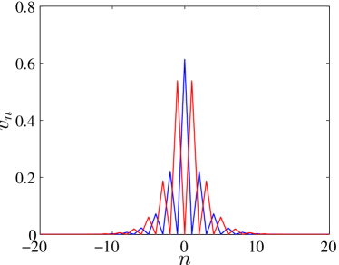
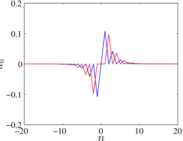
Figure 25: Profiles of both spinor components for the discrete 3-site (top) and 1-site (bottom) soliton (blue line) and its complimentary solution (red line). In all cases, $\omega=0.8$ and $\epsilon=0.5$ (i.e. close to the anti-continuum limit).

Let us explain below the general behavior for $\omega>1/3$. Outside this range, the solitary waves are generically unstable and hence we do not consider them further here. In the AC limit the individual sites are decoupled, and the eigenvalues of their respective $4\times 4$ matrices can be explicitly computed for both the cases of excited and non-excited sites. Thus it is straightforward to see from the stability matrix that in that limit, this three-site solution possesses 3 pairs of modes at $\lambda=0$, 3 pairs at $\lambda=\pm 2\omega{i}$, $(N-3)$ pairs at $\lambda=\pm i(1+\omega)$ and $(N-3)$ pairs at $\lambda=\pm i(1-\omega)$. When the coupling is switched on (see Fig. 26), the wave becomes exponentially unstable because of one among the 3 pairs at $\omega=0$ that detaches from the origin yielding a real eigenvalue pair in a similar way as occurs e.g. for the two-site structure in the DNLS equation cuevas-Kev09 . The other two vanishing eigenvalue pairs remain at the origin. In addition, the eigenmodes at $\lambda=\pm 2\omega{i}$ detach into three pairs that will subsequently collide with the essential spectrum; let us denote those modes as A, B, C (from upper to lower imaginary part of the eigenvalue). Mode C remains exactly at $\lambda=\pm 2\omega{i}$ for every coupling. Notice that mode C is always below the essential spectrum for $\omega<1/3$. The imaginary part of the eigenvalue of mode A rapidly increases entering the non-embedded spectrum at the point where the real part of the eigenvalue responsible for the exponential instability reaches its maximum. The exponential instability mentioned previously disappears close to (but not at) the point where mode C enters the embedded spectrum. However, when the coupling increases, the exponential instability appears again with a similar (non-monotonic) behavior as the previous one, except for the presence of smaller growth rates and of a slower decrease in the growth rate (past the point of the maximal growth rate). The most complex parametric dependence is the one experienced by mode B. The latter enters the embedded spectrum for a value of $\epsilon$ higher than that for which mode C enters therein. Then, the system becomes oscillatorily unstable and undergoes a Hopf bifurcation (in the case of finite systems, due to the quantization of the continuous spectrum, this translates into a series of instability bubbles; for a similar scenario in the DNLS see e.g. cuevas-JK99 ). As a consequence, there are many oscillations in the real part of mode B when the coupling is high; the amplitude of those oscillations decreases when the system size increases, as shown in the inset of bottom right panel of Fig. 26. When the frequency increases (say $\omega\gtrsim 0.67$) the real part of mode B does not asymptote to a nearly constant value as the coupling strength increases, but, on the contrary, a series of oscillation bubbles around 0 appears (see top panels of Fig. 26).

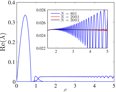
Figure 26: Dependence of the stability eigenvalues with respect to the coupling $\epsilon$ for discrete 3-site solitons with $\omega=0.8$ (top) and $\omega=0.6$ (bottom). Only the positive real and imaginary parts of the eigenvalues are shown. The size of the system is $N=801$. In the top left panel, letters (A, B, C) indicate the three relevant modes whose properties are indicated in the text. In the top right, the inset is a magnification of the relevant $\mathrm{Re}(\lambda)$ shown in the figure but at a different scale. The inset in the bottom right panel shows the oscillations of the growth rate for different system sizes when $\omega=0.6$. Notice that oscillation amplitude decreases rapidly as the number of lattice nodes increases.

A complementary scenario is experienced by the two-site soliton, given in the AC limit by $u_{n}=0\ \forall$ $n$ and $v_{0}=v_{1}=\sqrt{1-\omega}$, $v_{n}=0$ elsewhere (see the red line on the top panels of Fig. 25). At this limit, the 2-site structure possesses 2 pairs of modes at $\lambda=0$, 2 pairs at $\lambda=\pm 2\omega{i}$, $(N-2)$ pairs at $\lambda=\pm i(1+\omega)$ and $(N-2)$ pairs at $\lambda=\pm i(1-\omega)$. When the coupling is switched on (see Fig. 27), the structure remains stable because of the persistence of both pairs at $\lambda=0$. Mode A does not exist for this case; on the other hand, the oscillatory instabilities caused by mode B also exist for the 2-site case. When increasing the coupling, the solitary wave experiences a bifurcation leading to an exponential instability and becomes unstable, contrary to the 3-site soliton (notice that in typical Klein–Gordon and – e.g. saturable – DNLS settings, such stability exchanges take place between 2-site and 1-site breathers or solitary waves cuevas-Aub06 ; cuevas-HMSK04 ; cuevas-MCKC06 ). Here, there are exponential stability exchanges between 2-site and 3-site solitons, although the bifurcations of the two families of solutions do not perfectly coincide (nevertheless, in a number of such exchanges, the corresponding stabilization/destabilization thresholds are fairly proximal). This scenario is summarized in the left panel of Fig. 28. We should note in passing that these near-exchanges of stability suggest a scenario similar to the ones occurring e.g. in the saturable or cubic-quintic DNLS model where the near-exchange of stability of the 1- and 2-site solitons (in that case) is mediated through a series of pitchfork and reverse pitchfork bifurcations of asymmetric solution branches cuevas-CTCM06 ; cuevas-VJ06 .

Figure 27: Same as Fig. 26 but for the case of discrete 2-site solitons.

Figure 28: $\epsilon$ vs $\omega$ plane where different unstable regimes for discrete 3-site and 2-site (left) and 1-site solitons (right) are displayed. 3-site solitons are unstable inside the regions with blue edges of the left panel, whereas 2-site solitons are unstable inside the red lines. Above the black lines, both 3-site and 2-site solutions are oscillatorily unstable. 1-site solitons are exponentially unstable above the blue line of right panel, and stable below this line.

There is an interesting kind of solution that also exists from the AC limit and can be extended all the way to the continuum limit, namely the one-site soliton (see bottom panels of Fig. 25). This has the following property which is, in fact, preserved upon continuation for any value of the coupling (see bottom panels of Fig. 29): $v_{n}=0$ for odd $n$ and $u_{n}=0$ for even $n$; however, the charge density of the soliton is qualitatively different from that of the three-site solitons. In the AC limit $\epsilon=0$, $v_{0}=\sqrt{1-\omega}$, and $v_{n}=0$ for the rest of sites (with $u_{n}=0\ \forall$ $n$). The form of this solution can be identified as we approach the continuum limit, by transforming the discrete NLD equation (46) into the new set of equations:

$$\begin{split}\epsilon(u_{n+1}-u_{n-1})-v_{n}^{3}+(1-\omega)v_{n}=&0,\ \\ \epsilon(v_{n+2}-v_{n})+u_{n+1}^{3}+(1+\omega)u_{n+1}=&0,\end{split}$$ (47)

for even $n$. There, by neglecting the irrelevant (in this setting) inactive odd sites for one of the fields, and the even ones for the other, the envelope of the solitary waves can be seen to approach the homoclinic orbits of the following system of ODEs that is found by obtaining the continuum limit of (47):

$$\begin{split}\partial_{x}v=&-u^{3}-(1+\omega)u,\\ \partial_{x}u=&v^{3}-(1-\omega)v.\end{split}$$ (48)

Equation (48), which possesses homoclinic solutions for a wide range of frequencies $\omega$, is tantamount to the Dirac equation with Lorentz-symmetry-breaking nonlinearity appearing in models of binary waveguide arrays cuevas-TLB14 or graphene nanoribbons cuevas-HWC15 .

Figure 29: (Left) The spinor components of a discrete 1-site (blue) and 3-site solitons (red) with $\omega=0.8$ and $\epsilon=5$ (i.e. close to the continuum limit). (Right) Charge density $\rho_{n}=|u_{n}|^{2}+|v_{n}|^{2}$ for the solitary waves at the left. It is clear that the 1-site soliton does not asymptote to the 3-site soliton, but rather to a different envelope which is an homoclinic solution of (48).

The spectrum of the one-site solitons at $\epsilon=0$ consists of a single pair of eigenvalues at $\lambda=0$ and another single pair at $\lambda=\pm 2\omega{i}$; apart from these, there are $N-1$ pairs at $\lambda=\pm i(1+\omega)$ and $\lambda=\pm i(1-\omega)$. When the coupling is switched on, as there is only a single pair of eigenmodes at $\lambda=0$, the solitary wave does not experience exponential instabilities; in addition, the non-existence of mode B prevents the existence of destabilizing Hopf bifurcations arising in 3-site and 2-site solitons (see Fig. 30). The only observed instability is an exponential one arising for a finite value of coupling and caused by a mode that bifurcates from the essential spectrum as the coupling strength increases; the growth rate of this bifurcation depends non-monotonically on $\epsilon$ and tends asymptotically to zero when reaching the continuum limit. Similar to the 3-site structures, there is a complementary family of solitary waves consisting of 2-site structures with a hole in between, characterized by $v_{0}=v_{2}$ (see red line in the bottom panels of Fig. 25).

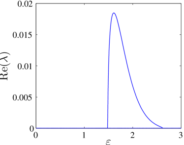
Figure 30: Same as Fig. 26 but for the case of discrete 1-site solitons.

We close this section by mentioning that a brief study of the dynamics of unstable discrete solitary waves was performed in cuevas-CKS15 . As stated therein, a systematic classification of the dynamical implications of the different identified instabilities and of the various possible configurations is a fairly extensive undertaking and deserves a separate numerical investigation in its own right.

0.8 $\mathcal{P}\mathcal{T}$-symmetric Nonlinear Dirac equation

This section is devoted to the existence, stability, and dynamics of solitary waves in a modified 1D Soler model where an additional parity-time symmetry preserving perturbation has been introduced.

0.8.1 $\mathcal{P}\mathcal{T}$ symmetry and Nonlinear Dirac equation

The study of open systems bearing gain and loss (especially so in a balanced form) is a topic that has emerged over the past two decades as a significant theme of study cuevas-Ben07 ; cuevas-BFGJ12 ; cuevas-FJZ08 ; cuevas-MECM11 . While the realm of $\mathcal{P}\mathcal{T}$-symmetry introduced by Bender and collaborators was originally intended as an alternative to the standard Hermitian quantum mechanics, its most canonical realizations (beyond the considerable mathematical analysis of the theme in its own right at the level of operators and spectral theory in mathematical physics) emerged elsewhere in physics. More specifically, in optical systems cuevas-RDM05 ; cuevas-KGM08 ; cuevas-MECM08 the analogy between the paraxial approximation of Maxwell’s equations and the Schrödinger equation formed the basis on which the possibility of $\mathcal{P}\mathcal{T}$-symmetric realizations initially in optical waveguide experiments was proposed and then experimentally implemented cuevas-GSD+09 ; cuevas-RME+10 ; cuevas-RBM+12 . The success of this program motivated further additional initiatives in other directions of experimental interest, including, but not limited to, $\mathcal{P}\mathcal{T}$-symmetric electronic circuits cuevas-SLZ+11 ; cuevas-SLL+12 , mechanical systems cuevas-BBPS13 and whispering-gallery microcavities cuevas-POL+14 . Our aim in this Section is to present a connection between the budding area of research of $\mathcal{P}\mathcal{T}$-symmetric systems and the nonlinear Dirac equation. To this aim, we choose a generalized $\mathcal{P}\mathcal{T}$-symmetric 1D Soler model, which in covariant form reads as follows:

$$\left(i\gamma^{\mu}\partial_{\mu}-m+g\left(\bar{\psi}\psi\right)^{k}+\gamma\gamma^{5}\right)\psi=0.$$ (49)

Alternatively, written in the standard form as a function of the bispinor components $\psi=[\psi_{1}(x),\psi_{2}(x)]^{T}$ cuevas-CKS+16 , the equations assume the following form:

$$\begin{split}i\partial_{t}\psi_{1}&=\,\,\partial_{x}\psi_{2}-g(|\psi_{1}|^{2}-|\psi_{2}|^{2})^{k}\psi_{1}+m\psi_{1}+i\gamma\psi_{2},\\ i\partial_{t}\psi_{2}&=-\partial_{x}\psi_{1}+g(|\psi_{1}|^{2}-|\psi_{2}|^{2})^{k}\psi_{2}-m\psi_{2}+i\gamma\psi_{1}.\end{split}$$ (50)

Equations (50) are $\mathcal{P}\mathcal{T}$-symmetric because they are invariant under the transformation

$${\mathcal{P}}:\;x\rightarrow-x,\qquad\psi_{1}\rightarrow\psi_{1},\qquad\psi_{2}\rightarrow-\psi_{2}$$

and

$${\mathcal{T}}:\;t\rightarrow-t,\qquad i\rightarrow-i,\qquad\psi_{1}\rightarrow\psi_{1},\qquad\psi_{2}\rightarrow\psi_{2}.$$

This transformation assumes that $\psi_{1}(t,x)$ is spatially even and that $\psi_{2}(t,x)$ is spatially odd. The key addition to this model in comparison to the original Soler model (7) is the inclusion of the gain-loss term proportional to $\gamma$ in the (implicit) form of the Dirac matrix $\gamma^{5}$ (cf. cuevas-Ben07 ) multiplying the spinor $\psi$ in (49). In our case of two-component spinors, the role of $\gamma^{5}$ is played by the Pauli matrix $\sigma_{1}$ (1). We note in passing that in its linear form, the model can be converted under a suitable transformation (associated with the so-called $\mathcal{C}$-operator) to a Hamiltonian one with a reduced mass of $\tilde{m}=\sqrt{m^{2}-\gamma^{2}}$ cuevas-Ben07 ; cuevas-BJR05 . It is straightforward to see that in the linear case (of $g=0$), plane waves $\psi_{1}(t,x)=Ae^{i(\kappa x-\omega t)}$ and $\psi_{2}(t,x)=iBe^{i(\kappa x-\omega t)}$ are solutions provided the dispersion relation $\omega=\pm\sqrt{m^{2}+\kappa^{2}-\gamma^{2}}$ is satisfied. Not only does the above formula have the characteristic Dirac form, but it also is consistent with the equivalence of the linear $\mathcal{P}\mathcal{T}$-Dirac equation with effective mass $\tilde{m}=\sqrt{m^{2}-\gamma^{2}}$, as per the above discussion. In the present $\mathcal{P}\mathcal{T}$-NLD we have been unable to identify explicit stationary solitary waves in the massive $m\neq 0$ case, so we must rely on numerical analysis. In the same vein, it does not appear to be straightforward to generalize the transformation of cuevas-Ben07 ; cuevas-BJR05 to the present nonlinear setting. To determine the stability of stationary solitary wave solutions, we consider infinitesimal perturbations of the form:

$$\begin{split}\psi_{1}(t,x)&=e^{-i\omega t}\left[v(x)+\delta(a_{1}(x)e^{\lambda t}+b_{1}^{*}(x)e^{\lambda^{*}t})\right],\\ \psi_{2}(t,x)&=e^{-i\omega t}\left[u(x)+\delta(a_{2}(x)e^{\lambda t}+b_{2}^{*}(x)e^{\lambda^{*}t})\right],\end{split}$$

where $\delta$ denotes a formal small parameter. The relevant linearization equations are derived to order ${\rm O}(\delta)$ [by substitution of the above Ansatz into Eqs. (50)] and are subsequently solved as a matrix eigenvalue problem

$$\lambda[a_{1}(x),a_{2}(x),b_{1}(x),b_{2}(x)]^{T}=\mathcal{M}[a_{1}(x),a_{2}(x),b_{1}(x),b_{2}(x)]^{T},$$

with $\mathcal{M}$ being

$$\mathcal{M}=\left(\begin{array}[]{cc}L_{1}&L_{2}\\ \\ -L_{2}^{*}&-L_{1}^{*}\end{array}\right)-i\gamma\left(\begin{array}[]{cc}\gamma^{5}&0\\[8.61108pt] 0&\gamma^{5}\end{array}\right)$$

and

$$\begin{split}L_{1}&=\left(\begin{array}[]{cc}f(|v|^{2}-|u|^{2})-m+\Lambda&-\partial_{x}\\ \\ \partial_{x}&m-f(|v|^{2}-|u|^{2})+\Lambda\end{array}\right)\\ &+f^{\prime}(|v|^{2}-|u|^{2})\left(\begin{array}[]{cc}|v|^{2}&-v^{*}u\\ \\ -v^{*}u&|u|^{2}\end{array}\right),\\ L_{2}&=f^{\prime}(|v|^{2}-|u|^{2})\left(\begin{array}[]{cc}v^{2}&-vu\\ \\ -vu&u^{2}\end{array}\right).\end{split}$$

From the dynamical equations (50) it is straightforward to show that the charge is not preserved. Instead, the following “moment equation” is satisfied:

$$\frac{dQ}{dt}=4\gamma\int\mathrm{Re}(V^{*}U)\,dx\,.$$ (51)

Note that in the case of a standing wave state, $dQ/dt=0$ and charge is conserved. Although the charge is not generally conserved, remarkably there is a conserved quantity in the form of the energy:

$$E=\frac{1}{2}\int\left[\psi_{1}^{*}\partial_{x}\psi_{2}-\psi_{2}^{*}\partial_{x}\psi_{1}+m(|\psi_{1}|^{2}-|\psi_{2}|^{2})-\frac{g}{k+1}[|\psi_{1}|^{2}-|\psi_{2}|^{2}]^{k+1}\right]\,dx\,.$$

Notice that there is no $\gamma$ dependence in this formula. As a matter of fact, this is the same definition for the energy as in the $\gamma=0$ limit (cf. Eq.(4)). But, intriguingly, $dE/dt=0$ even for $\gamma\neq 0$. This is rather unusual in our experience in $\mathcal{P}\mathcal{T}$-symmetric models and is effectively related to the special form of introducing $\mathcal{P}\mathcal{T}$-symmetry through the matrix $\gamma^{5}$. We note that in this form, it is not transparent (unlike e.g. in the Schrödinger $\mathcal{P}\mathcal{T}$-symmetric models cuevas-Ben07 ) which component corresponds to the gain and which one to the loss. Effectively, isolating the time-dependence and the $\gamma$-dependent term in the equations (i.e., $i\partial_{t}\psi_{1}=i\gamma\psi_{2}$ and $i\partial_{t}\psi_{2}=i\gamma\psi_{1}$ and momentarily ignoring the rest of the terms), it appears as if both components bear both gain and loss.

0.8.2 Numerical results

In the numerical computations presented herein, we have utilized spectral collocation methods in order to approximate the spatial derivatives of Eq. (50). As discussed in Subsection 3.2, the Chebyshev collocation is, arguably, the most suitable method for approximating the relevant derivatives as it gives a better spectral accuracy. However, because of the particular ($\mathcal{P}\mathcal{T}$-symmetric) structure of the system, the implementation of fixed-point methods, requires a high amount of computer memory which poses implementation challenges. Furthermore, the method has the drawback that the double humped solitary waves, cannot be well resolved (i.e. the humps cannot be observed) because of the Chebyshev collocation including more points at the edge of the system in comparison to the center. Consequently, in what follows, a Fourier collocation scheme has been implemented. In suitable limit cases, we have checked that the results are similar for the different implementations and that no extra spurious eigenmodes arise in comparison to the standard case. We note that hereafter we will focus on the case of $k=1$ for our numerical implementation and $g=m=1$ has been fixed. The first numerical result found by studying the standing wave solution is the $\mathcal{P}\mathcal{T}$ transition point. We have checked that this transition takes place when $\gamma=\gamma_{\mathrm{PT}}$ with $\gamma_{\mathrm{PT}}=\sqrt{1-\omega^{2}}$; notice that this is consonant with our analytical prediction from the previous section in the case of wavenumber $\kappa=0$. Fig. 31 shows the profile of typical solitary waves with nonzero $\gamma$. Importantly, we have observed (see Fig. 32) that the relevant perturbation does not introduce instabilities to our system. The relevant spectrum features a zero eigenvalue of algebraic multiplicity four and geometric multiplicity two. This is present in the spectrum of the linearized equation due to the $\mathbf{U}(1)$ symmetry and due to the translational symmetry, which are both preserved when $\gamma\neq 0$, hence both the algebraic and geometric multiplicity of this eigenvalue are preserved for all values of $\gamma$, as is the presence of two generalized eigenvectors. The spectrum also features the ubiquitous eigenvalues $\lambda=\pm 2\omega{i}$ which is due to the $\mathbf{SU}(1,1)$-invariance, and is also preserved for any $\gamma$; the relevant eigenvalue, which persists under variations of $\gamma$, can be discerned in the left panel of Fig. 32. For the rest of the spectrum we note that, as discussed in Section 4, eigenvalues with nonzero real part can only be born in the embedded spectrum. Here, however, all the eigenvalues remain inside this interval for all $\gamma$, as illustrated in Fig. 32, solely tending towards $0$, as $\gamma$ approaches $\gamma_{\mathrm{PT}}$.

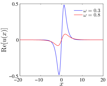
Figure 31: Real and imaginary part of each spinor component for $\mathcal{P}\mathcal{T}$-symmetric solitary waves with $\omega=0.8$ and $\omega=0.3$. Here $\gamma=0.3$ in every case. The charge density of the solitary wave is depicted in the bottom panel.

Figure 32: Imaginary part of the eigenvalues dependence for $\mathcal{P}\mathcal{T}$-symmetric solitary waves with $\omega=0.3$ (left) and $\omega=0.8$ (right). Notice the existence on the left panel of a constant eigenvalue at $\lambda=2\omega{i}$. Notice also the approach of the eigenvlaues towards $0$, as per the discussed collision with the linear limit.

Notice that the $\mathcal{P}\mathcal{T}$-transition is caused by the nonlinear solutions colliding with (or degenerating into) linear modes. This fact can also be confirmed in the plots of Fig. 33, where the charge and energy tend to zero (while a width diagnostic  of the solution diverges) when the transition point is reached (actually, we have not been able to reach this point exactly, as the solitary wave width increases drastically when approaching this point). It should be noted here that this is a distinct phenomenology in comparison to the NLS counterpart of the model. In the latter, typically at the $\mathcal{P}\mathcal{T}$-phase transition a stable (center) and an unstable (saddle) solution collide and disappear in a saddle-center bifurcation. Here, a fundamentally different scenario arises through the degeneration of the nonlinear modes into linear ones. In Fig. 34, we provide two-parameter diagrams of the relevant solutions as a function of the frequency $\omega$ and the gain-loss parameter $\gamma$. The dependencies strongly suggest a “combined” monoparametric dependence on $\gamma^{2}+\omega^{2}$, although we have not been able to analytically identify solutions bearing this dependence.

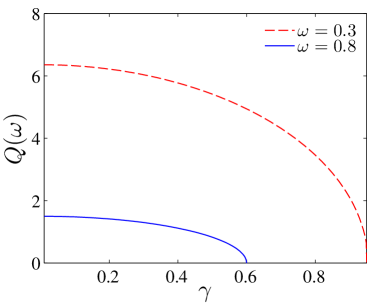
Figure 33: Energy, width, and charge dependence with respect to $\gamma$ of the $\mathcal{P}\mathcal{T}$-symmetric solitary waves with $\omega=0.8$ and $\omega=0.3$.

Figure 34: Two-parameter diagram of the dependence of the width and energy of $\mathcal{P}\mathcal{T}$-symmetric solitary waves on the frequency $\omega$ and gain-loss parameter $\gamma$.

We now turn to the consideration of the dynamical evolution of solitary waves past the $\mathcal{P}\mathcal{T}$-transition point. As indicated above, given their generic stability for $\gamma<\gamma_{\mathrm{PT}}$, we do not consider the latter case. In the case of $\gamma>\gamma_{\mathrm{PT}}$, we have firstly taken as initial condition the solitary wave for $\omega=0.8$ and $\gamma=\gamma_{0}=0.59$ in the simulation with $\gamma=\gamma_{s}>\gamma_{\mathrm{PT}}=\sqrt{1-\omega^{2}}=0.6$. We observe that if $\gamma_{s}$ is close enough to $\gamma_{\mathrm{PT}}$ (i.e., for a “shallow” quench), the density oscillates with a frequency that decreases with $\gamma_{s}-\gamma_{\mathrm{PT}}$ (see Figs. 35 and 36). Notice that the charge of the new solitary wave is always higher than the charge of the initial one and that the maximum charge increases with $\gamma_{s}$. Interestingly, in all of these case examples we find that the ($\gamma$-independent) energy ($E=0.2738$ for $\omega=0.8$) is very well conserved as shown in cuevas-CKS+16 . When the maximum charge is above a threshold (this occurs for $\gamma_{s}\gtrsim 0.995$, i.e., for a deep quench), the frequency of the new solitary wave tends to zero and the solution starts to grow indefinitely as shown in Fig. 37. If a smaller value of $\gamma_{0}$ is taken, the same phenomenology persists, but the indefinite growth emerges for a smaller value of $\gamma_{s}$. It was also confirmed in cuevas-CKS+16 that both the energy conservation law and the moment equation (51) for the charge are satisfied in the dynamics of $\mathcal{P}\mathcal{T}$-symmetric solitary waves. The same is true for the case of Fig. 37 where the charge grows exponentially (in the case shown in the figure, for which $\gamma_{s}=1$, approximately as $\exp(0.088t)$; although the characteristic growth rate depends on $\gamma_{s}$). Here, the solitary wave does not collapse, as its shape and width are preserved during the growth. Again, this type of growth appears to be very different than, say, the collapse in the Hamiltonian NLS model cuevas-SS99 . In the latter, the width decreases and the amplitude increases, whereas here the entire solution grows without changing its spatial distribution.

Figure 35: Dynamics for the $\mathcal{P}\mathcal{T}$-symmetric NLD using as initial condition the solitary wave with $\omega=0.8$ and $\gamma=0.59$, but evolving Eq. (50) for the value of $\gamma$ shown in the respective panels. Each panel shows the space-time evolution of the solitary wave density.

Figure 36: Same as Fig. 35 but showing the time evolution of the solitary wave charge. The red dashed line corresponds to the charge of the initial condition.

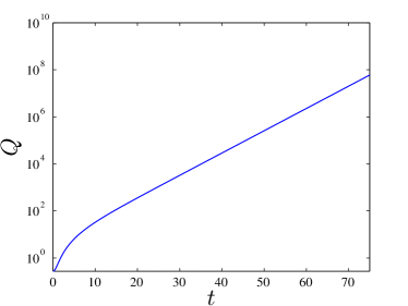
Figure 37: Dynamics for the $\mathcal{P}\mathcal{T}$-symmetric NLD using as initial condition the solitary wave with $\omega=0.8$ and $\gamma=0.59$, but evolving Eq. (50) for the value $\gamma=1$. The left panel shows the charge density at different times. The right panel shows the total charge as a function of time. One can clearly observe the (spatially independent) exponential growth of the waveform.

Let us mention that the waveform with oscillating charge is fairly generic when the quench is not sufficiently deep to cause an exponential growth. Remarkably, such solitary waves with oscillating charge can be obtained by performing an $\mathbf{SU}(1,1)$-transformation to a standard (one-frequency) solitary wave cuevas-Gal77 ; cuevas-DR79 . This type of solution for a standing wave of frequency $\tilde{\omega}$ is, in fact, intrinsically connected to the invariance of the eigenvalue $2\tilde{\omega}i$ (associated to eigenfrequency $2\tilde{\omega}$) in the spectrum. More specifically, these bi-frequency, oscillating charge coherent structures [which can be dubbed as $\mathbf{SU}(1,1)$-solitary waves] are of the form:

$$\begin{split}\psi_{1}(t,x)=&\alpha_{-}\tilde{v}(x)e^{-i\tilde{\omega}t}-i\alpha_{+}\tilde{u}^{*}(x)e^{i\tilde{\omega}t}\,,\\ \psi_{2}(t,x)=&\alpha_{-}\tilde{u}(x)e^{-i\tilde{\omega}t}-i\alpha_{+}\tilde{v}^{*}(x)e^{i\tilde{\omega}t}\,,\end{split}$$ (52)

with

$$\alpha_{\pm}\in\mathbb{C},\qquad|\alpha_{-}|^{2}-|\alpha_{+}|^{2}=1.$$

In this case, $\{\tilde{v}(x),\tilde{u}(x)\}$ is the standing wave solution with frequency $\tilde{\omega}$. Consequently, the charge oscillates with a frequency $2\tilde{\omega}$ as long as $\gamma\neq 0$. There is an $\mathbf{SU}(1,1)$-family of solutions for each value of $\gamma$ and $\tilde{\omega}$ which fulfills the same equations that the standing wave solutions satisfy. As a result, when $\gamma_{s}\neq\gamma_{0}$, an $\mathbf{SU}(1,1)$-solution with $\gamma=\gamma_{s}$ is apparently dynamically manifested. Since these periodic $\mathbf{SU}(1,1)$-solutions and the standing wave solutions only exist for $\gamma<m\equiv 1$, it is natural to expect that there are no nontrivial fixed points for the dynamics for $\gamma>1$, hence giving rise to the observed growth dynamics. We have confirmed that the dynamics observed, e.g., in Fig. 35 corresponds to $\mathbf{SU}(1,1)$-solutions. For instance, for the solitary wave with $\gamma_{0}=0.59$, $\omega=0.8$, when initializing it for $\gamma_{s}=0.9$, it spontaneously gives rise to an oscillatory state of the above form of equation (52) with $\tilde{\omega}=0.422$, $\alpha_{-}=1.0847$ and $\alpha_{+}=0.4201$. On the other hand, using a numerically exact (up to a prescribed tolerance) solution of our fixed point iteration scheme with a given frequency $\tilde{\omega}$ (for a desired $\gamma$), we can select values of $\alpha_{-}$ and $\alpha_{+}$ and the exact form of Eq. (52) in order to construct, at will, such bi-frequency $\mathbf{SU}(1,1)$-solutions. An example of this form is shown in Figs. 38 and 39 (even for $\gamma=0$) for $\tilde{\omega}=0.5$, $\alpha_{-}=1.0500$, and $\alpha_{+}=0.3202$.

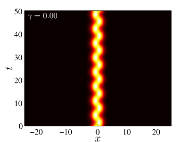
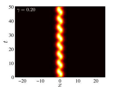
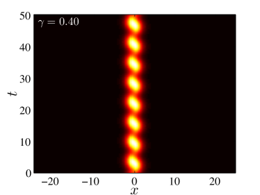
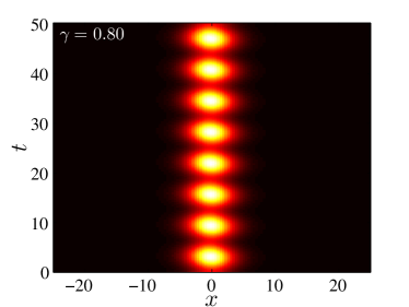
Figure 38: Dynamics for $\mathbf{SU}(1,1)$-solitary waves with $\tilde{\omega}=0.5$, $\alpha_{-}=1.0500$, $\alpha_{+}=0.3202$, and the value of $\gamma$ indicated in each panel [see Eq. (52)]. Each panel shows the space-time evolution of the solution density.

Figure 39: Same as Fig. 38 but showing the time evolution of the solution charge.

0.9 Summary and outlook

In the present work, we have discussed some of the principal properties of the nonlinear Dirac equation and its similarities, as well as differences, in comparison to its extensively studied cousin, namely the nonlinear Schrödinger equation. We have discussed nonlinear models that possess solitary wave solutions and vortices, and have placed particular emphasis on their spectral stability, also mentioning the orbital and asymptotic stability thereof and the corresponding issues that arise. We have seen that especially in higher dimensions the stability properties of solitary waves in the nonlinear Dirac equation can be fundamentally different from the NLS case, and may not feature collapse scenarios. Moreover, solitary waves may be spectrally stable for suitable parametric (i.e., frequency) regimes. For the three-dimensional case, the stability properties are just starting to be explored (in suitable subspaces), yet this problem is extremely interesting, also due to its connections with the dynamics. In the context of the latter, we explored some of the delicate features that arise from different types of discretizations (finite-difference, Fourier and Chebyshev spectral schemes) and the implications for the evolutionary dynamics. Generally, we hope to have exposed some of the significant complications arising in dynamically propagating such a system, especially when trying to do so for long time scales. From every perspective that we can think of, nonlinear Dirac systems pose significant challenges ahead of us. From the point of view of the mathematical analysis, understanding the spectral properties observed herein and their dynamical implications is already a formidable problem. Computing efficiently and systematically both the solutions and their linearization eigenvalues emerges as a significant and upcoming challenge. This is especially true in three spatial dimensions. Devising numerical schemes – possibly based on integrable (semi-discrete or genuinely discrete) variants of the model – could prove to be of paramount importance towards future robust computations of the dynamics. Finally, combining some of the cutting edge themes in nonlinear waves (such as for instance rogue waves cuevas-KPS09 ) with relevant scenarios involving Dirac-type nonlinear models opens another highly promising vein of research for future studies cuevas-DWA15 .

Acknowledgments

The research of Andrew Comech was carried out at the Institute for Information Transmission Problems of the Russian Academy of Sciences at the expense of the Russian Foundation for Sciences (project 14-50-00150). J.C.-M. thanks financial support from MAT2016-79866-R project (AEI/FEDER, UE). P.G.K. gratefully acknowledges the support of NSF-PHY-1602994, the Alexander von Humboldt Foundation, the Stavros Niarchos Foundation via the Greek Diaspora Fellowship Program, and the ERC under FP7, Marie Curie Actions, People, International Research Staff Exchange Scheme (IRSES-605096). This work was supported in part by the U.S. Department of Energy.

References

- (1) Ablowitz, M.J., Nixon, S.D., Zhu, Y.: Conical diffraction in honeycomb lattices. Phys. Rev. A 79, 053830 (2009)
- (2) Ablowitz, M.J., Prinari, B., Trubatch, A.D.: Discrete and continuous Nonlinear Schrödinger systems. Cambridge University Press, Cambridge (2004)
- (3) Ablowitz, M.J., Zhu, Y.: Evolution of Bloch-mode envelopes in two-dimensional generalized honeycomb lattices. Phys. Rev. A 82, 013840 (2010)
- (4) Achilleos, V., Frantzeskakis, D.J., Kevrekidis, P.G., Pelinovsky, D.E.: Matter-wave bright solitons in spin-orbit coupled Bose-Einstein condensates. Phys. Rev. Lett. 110, 264101 (2013)
- (5) Achilleos, V., Stockhofe, J., Kevrekidis, P.G., Frantzeskakis, D.J., Schmelcher, P.: Matter-wave dark solitons and their excitation spectra in spin-orbit coupled Bose-Einstein condensates. Europhys. Lett. 103(2), 20002 (2013)
- (6) Alexander, J., Gardner, R., Jones, C.: A topological invariant arising in the stability analysis of traveling waves. J. Reine Angew. Math 410, 167–212 (1990)
- (7) Alfimov, G.L., Kevrekidis, P.G., Konotop, V.V., Salerno, M.: Wannier functions analysis of the nonlinear Schrödinger equation with a periodic potential. Phys. Rev. E 66, 046608 (2002)
- (8) Alvarez, A., Soler, M.: Energetic stability criterion for a nonlinear spinorial model. Phys. Rev. Lett. 50, 1230–1233 (1983)
- (9) Alvarez, A., Soler, M.: Stability of the minimum solitary wave of a nonlinear spinorial model. Phys. Rev. D 34, 644–645 (1986)
- (10) Aubry, S.: Discrete Breathers: Localization and transfer of energy in discrete Hamiltonian nonlinear systems. Physica D 216, 1–30 (2006)
- (11) Barashenkov, I.V., Pelinovsky, D.E., Zemlyanaya, E.V.: Vibrations and oscillatory instabilities of gap solitons. Phys. Rev. Lett. 80, 5117–5120 (1998)
- (12) Bender, C.M.: Making sense of non-Hermitian Hamiltonians. Rep. Prog. Phys. 70, 947–1018 (2007)
- (13) Bender, C.M., Berntson, B.K., Parker, D., Samuel, E.: Observation of PT phase transition in a simple mechanical system. Am. J. Phys 81, 173–179 (2013)
- (14) Bender, C.M., Fring, A., Günther, U., Jones, H.: Special issue: Quantum physics with non-hermitian operators. J. Phys. A, Math Theor. 45(44), 020201 (2012)
- (15) Bender, C.M., Jones, H.F., Rivers, R.J.: Dual PT-symmetric quantum field theories. Phys. Lett. B 625, 333–340 (2005)
- (16) Berestycki, H., Lions, P.L.: Nonlinear scalar field equations. I. Existence of a ground state. Arch. Rational Mech. Anal. 82(4), 313–345 (1983)
- (17) Berkolaiko, G., Comech, A.: On spectral stability of solitary waves of nonlinear dirac equation in 1D. Math. Model. Nat. Phenom. 7, 13–31 (2012)
- (18) Berkolaiko, G., Comech, A., Sukhtayev, A.: Vakhitov-Kolokolov and energy vanishing conditions for linear instability of solitary waves in models of classical self-interacting spinor fields. Nonlinearity 28(3), 577–592 (2015)
- (19) Berthier, A., Georgescu, V.: On the point spectrum of Dirac operators. J. Funct. Anal. 71(2), 309–338 (1987)
- (20) Bjorken, J., Drell, S.: Relativistic quantum mechanics. McGraw-Hill, New York (1964)
- (21) Blanchard, P., Stubbe, J., Vázquez, L.: Stability of nonlinear spinor fields with application to the Gross-Neveu model. Phys. Rev. D 36, 2422–2428 (1987)
- (22) Bogolubsky, I.L.: On spinor soliton stability. Phys. Lett. A 73, 87–90 (1979)
- (23) Bournaveas, N.: Local existence for the Maxwell-Dirac equations in three space dimensions. Comm. Partial Differential Equations 21(5-6), 693–720 (1996)
- (24) Boussaïd, N.: Stable directions for small nonlinear Dirac standing waves. Comm. Math. Phys. 268(3), 757–817 (2006)
- (25) Boussaïd, N.: On the asymptotic stability of small nonlinear Dirac standing waves in a resonant case. SIAM J. Math. Anal. 40(4), 1621–1670 (2008)
- (26) Boussaïd, N., Comech, A.: On spectral stability of the nonlinear Dirac equation. J. Funct. Anal. 271(6), 1462–1524 (2016)
- (27) Boussaïd, N., Comech, A.: Spectral stability of weakly relativistic solitary waves of the Dirac equation with the Soler-type nonlinearity (2016)
- (28) Boussaïd, N., Comech, A.: Spectral stability of weakly relativistic solitary waves of the Dirac equation with the Soler-type nonlinearity (2017). To appear
- (29) Boussaïd, N., Cuccagna, S.: On stability of standing waves of Nonlinear Dirac equations. Commun. Part. Diff. Eq. 37, 1001–1056 (2012)
- (30) Boyd, J.P.: Chebyshev and Fourier spectral methods, 2nd. edition edn. Dover, New York (2001)
- (31) Braun, O.M., Kivshar, Y.S.: The Frenkel-Kontorova Model. Springer Nature (2004)
- (32) Buslaev, V.S., Perel′man, G.S.: On the stability of solitary waves for nonlinear Schrödinger equations. In: Nonlinear evolution equations, Amer. Math. Soc. Transl. Ser. 2, vol. 164, pp. 75–98. Amer. Math. Soc., Providence, RI (1995)
- (33) Candy, T.: Global existence for an critical nonlinear Dirac equation in one dimension. Adv. Differential Equations 16(7-8), 643–666 (2011)
- (34) Carretero-González, R., Talley, J.D., Chong, C., Malomed, B.A.: Multistable solitons in the cubic-quintic discrete nonlinear Schrödinger equation. Physica D 216, 77–89 (2006)
- (35) Cazenave, T., Lions, P.L.: Orbital stability of standing waves for some nonlinear Schrödinger equations. Comm. Math. Phys. 85(4), 549–561 (1982)
- (36) Cazenave, T., Vazquez, L.: Existence of localized solutions for a classical nonlinear Dirac field. Commun. Math. Phys. 105, 35–47 (1986)
- (37) Chugunova, M., Pelinovsky, D.: Block-diagonalization of the symmetric first-order coupled-mode system. SIAM J. Appl. Dyn. Syst. 5(1), 66–83 (2006)
- (38) Coleman, S.: Quantum sine-Gordon equation as the massive Thirring model. Phys. Rev. D 11, 2088–2097 (1975)
- (39) Comech, A., Guan, M., Gustafson, S.: On linear instability of solitary waves for the nonlinear Dirac equation. Ann. I. H. Poincaré – AN 31, 639–654 (2014)
- (40) Comech, A., Phan, T.V., Stefanov, A.: Asymptotic stability of solitary waves in generalized Gross-Neveu model. Ann. Inst. H. Poincaré – AN 34, 157–196 (2017)
- (41) Comech, A., Stuart, D.: Small solitary waves in the Dirac-Maxwell system (2012). ArXiv:1210.7261
- (42) Conduit, G.J.: Line of Dirac monopoles embedded in a Bose-Einstein condensate. Phys. Rev. A 86, 021605(R) (2012)
- (43) Contreras, A., Pelinovsky, D.E., Shimabukuro, Y.: L2 orbital stability of Dirac solitons in the massive Thirring model. Commun. Part. Diff. Eq. 41, 227–255 (2016)
- (44) Cooper, F., Khare, A., Mihaila, B., Saxena, A.: Solitary waves in the nonlinear Dirac equation with arbitrary nonlinearity. Phys. Rev. E 82, 036604 (2010)
- (45) Cuccagna, S., Tarulli, M.: On stabilization of small solutions in the nonlinear Dirac equation with a trapping potential. J. Math. Anal. Appl. 436(2), 1332–1368 (2016)
- (46) Cuevas-Maraver, J., Kevrekidis, P., Saxena, A., Cooper, F., Mertens, F.: Solitary waves in the nonlinear Dirac equation at the continuum limit: Stability and dynamics. In: Ordinary and Partial Differential Equations. Nova Science Publishers, New York (2015)
- (47) Cuevas-Maraver, J., Kevrekidis, P.G., Saxena, A.: Solitary waves in a discrete nonlinear Dirac equation. J. Phys. A: Math. Theor. 48, 055204 (2015)
- (48) Cuevas-Maraver, J., Kevrekidis, P.G., Saxena, A., Comech, A., Lan, R.: Stability of solitary waves and vortices in a 2D nonlinear Dirac model. Phys. Rev. Lett. 116, 214101 (2016)
- (49) Cuevas-Maraver, J., Kevrekidis, P.G., Saxena, A., Cooper, F., Khare, A., Comech, A., Bender, C.M.: Solitary waves of a PT-symmetric Nonlinear Dirac equation. IEEE J. Sel. Top. Quantum Electron. 22, 5000109 (2016)
- (50) Cuevas-Maraver, J., Kevrekidis, P.G., Williams, F. (eds.): The sine-Gordon Model and its Applications. Springer International Publishing (2014)
- (51) Dalibard, J., Gerbier, F., Juzeliunas, G., Öhberg, P.: Colloquium: Artificial gauge potentials for neutral atoms. Rev. Mod. Phys. 83, 1523–1543 (2011)
- (52) Darby, D., Ruijgrok, T.W.: A noncompact gauge group for the Dirac equation. Acta Phys. Polon. B 10, 959–973 (1979)
- (53) Dauxois, T., Peyrard, M.: Physics of solitons. Cambridge University Press, Cambridge (2006)
- (54) De Wit, B., Smith, J.: Field Theory in Particle Physics. North Holland Physics Publishing, New York (1986)
- (55) Degasperis, A., Wabnitz, S., Aceves, A.: Bragg grating rogue wave. Phys. Lett. A 379, 1067–1070 (2015)
- (56) Derrick, G.H.: Comments on nonlinear wave equations as models for elementary particles. J. Math. Phys. 5, 1252–1254 (1964)
- (57) Dirac, P.: The quantum theory of the electron. I. Proc. R. Soc. Lond. A 117, 610–624 (1928)
- (58) Dormand, J.R., Prince, P.J.: A family of embedded runge-kutta formulae. J. Comp. Appl. Math. 6, 19–26 (1980)
- (59) Escobedo, M., Vega, L.: A semilinear Dirac equation in for . SIAM J. Math. Anal. 28(2), 338–362 (1997)
- (60) Esteban, M.J., Georgiev, V., Séré, É.: Stationary solutions of the Maxwell-Dirac and the Klein-Gordon-Dirac equations. Calc. Var. Partial Differential Equations 4(3), 265–281 (1996)
- (61) Esteban, M.J., Lewin, M., Séré, É.: Variational methods in relativistic quantum mechanics. Bull. Amer. Math. Soc. (N.S.) 45(4), 535–593 (2008)
- (62) Esteban, M.J., Séré, E.: Stationary states of the nonlinear Dirac equation: A variational approach. Commun. Math. Phys. 171, 323–350 (1995)
- (63) Esteban, M.J., Séré, É.: Solutions of the Dirac-Fock equations for atoms and molecules. Comm. Math. Phys. 203(3), 499–530 (1999)
- (64) Esteban, M.J., Séré, E.: Nonrelativistic limit of the Dirac-Fock equations. Ann. Henri Poincaré 2(5), 941–961 (2001)
- (65) Esteban, M.J., Séré, É.: Dirac-Fock models for atoms and molecules and related topics. In: XIVth International Congress on Mathematical Physics, pp. 21–28. World Sci. Publ., Hackensack, NJ (2005)
- (66) Evans, J.: Nerve axon equations, I: Linear approximations. Indiana U. Math. J. 21, 877–955 (1972)
- (67) Evans, J.: Nerve axon equations, II: Stability at rest. Indiana U. Math. J. 22, 75–90 (1972)
- (68) Evans, J.: Nerve axon equations, III: Stability of the nerve impulse. Indiana U. Math. J. 22, 577–594 (1972)
- (69) Evans, J.: Nerve axon equations, IV: The stable and unstable impulse. Indiana U. Math. J. 24, 1169–1190 (1975)
- (70) Fedosov, B.V.: Index theorems. In: Partial Differential Equations, VIII Encyclopaedia Math. Sci., vol. 65. Springer Verlag, Berlin (1996)
- (71) Feng, B., Sugino, O., Liu, R.Y., Zhang, J., Yukawa, R., Kawamura, M., Iimori, T., Kim, H., Hasegawa, Y., Li, H., Chen, L., Wu, K., Kumigashira, H., Komori, F., Chiang, T.C., Meng, S., Matsuda, I.: Dirac fermions in borophene. Phys. Rev. Lett. 118, 096401 (2017)
- (72) Fialko, O., Brand, J., Zülicke, U.: Hidden long-range order in a two-dimensional spin-orbit coupled bose gas. Phys. Rev. A 85, 051605(R) (2012)
- (73) Finkelstein, R., Lelevier, R., Ruderman, M.: Nonlinear spinor fields. Phys. Rev. 83, 326–332 (1951)
- (74) Fring, A., Jones, H., Znojil, M.: Papers dedicated to the subject of the 6th international workshop on pseudo-Hermitian Hamiltonians in quantum physics (PHHQPVI). J. Phys. A: Math Theor. 41(44) (2008)
- (75) Galindo, A.: A remarkable invariance of classical Dirac Lagrangians. Lett. Nuovo Cimento 20, 210–212 (1977)
- (76) Georgiev, V., Ohta, M.: Nonlinear instability of linearly unstable standing waves for nonlinear Schrödinger equations. J. Math. Soc. Japan 64(2), 533–548 (2012)
- (77) Grillakis, M., Shatah, J., Strauss, W.: Stability theory of solitary waves in the presence of symmetry. I. J. Funct. Anal. 74(1), 160–197 (1987)
- (78) Gross, D.J., Neveu, A.: Dynamical symmetry breaking in asymptotically free field theories. Phys. Rev. D 10, 3235–3253 (1974)
- (79) Gross, L.: The Cauchy problem for the coupled Maxwell and Dirac equations. Comm. Pure Appl. Math. 19, 1–15 (1966)
- (80) Guo, A., Salamo, G.J., Duchesne, D., Morandotti, R., Volatier-Ravat, M., Aimez, V., Siviloglou, G.A., Christodoulides, D.N.: Observation of PT-symmetry breaking in complex optical potentials. Phys. Rev. Lett. 103, 093902 (2009)
- (81) Haddad, L.H., Carr, L.D.: The nonlinear Dirac equation in Bose-Einstein condensates: vortex solutions and spectra in a weak harmonic trap. New J. Phys. 17, 113011 (2015)
- (82) Haddad, L.H., O’Hara, K.M., Carr, L.D.: Nonlinear Dirac equation in Bose-Einstein condensates: preparation and stability of relativistic vortices. Phys. Rev. A 91, 043609 (2015)
- (83) Haddad, L.H., Weaver, C.M., Carr, L.D.: The nonlinear Dirac equation in Bose-Einstein condensates: I. Relativistic solitons in armchair nanoribbon optical lattices. New J. Phys. 17, 063044 (2015)
- (84) Hadzievski, L., Maluckov, A., Stepić, M., Kip, D.: Power controlled soliton stability and steering in lattices with saturable nonlinearity. Phys. Rev. Lett. 93, 033901 (2004)
- (85) Hairer, E., Nørsett, S.P., Wanner, G.: Solving Ordinary Differential Equations I, Springer Series in Computational Mathematics, vol. 8. Springer, Berlin (1993)
- (86) Hamner, C., Zhang, Y., Khamehchi, M.A., Davis, M.J., Engels, P.: In a one-dimensional optical lattice, spin-orbit-coupled Bose-Einstein condensates. Phys. Rev. Lett. 114, 070401 (2014)
- (87) Heisenberg, W.: Quantum theory of fields and elementary particles. Rev. Mod. Phys. 29, 269–278 (1957)
- (88) Herring, G., Carr, L.D., Carretero-González, R., Kevrekidis, P.G., Frantzeskakis, D.J.: Radially symmetric nonlinear states of harmonically trapped Bose-Einstein condensates. Phys. Rev. A 77, 023625 (2008)
- (89) Huh, H.: Global solutions to Gross-Neveu equation. Lett. Math. Phys. 103(8), 927–931 (2013)
- (90) Ivanenko, D.D.: Notes to the theory of interaction via particles. Sov. Phys. JETP 13, 141 (1938)
- (91) Jensen, A., Kato, T.: Spectral properties of Schrödinger operators and time-decay of the wave functions. Duke Math. J. 46(3), 583–611 (1979)
- (92) Johansson, M., Kivshar, Y.S.: Discreteness-induced oscillatory instabilities of dark solitons. Phys. Rev. Lett. 82, 85–88 (1999)
- (93) Jones, C.: Stability of the travelling wave solutions of the Fitzhugh–Nagumo system. Trans. AMS 286(2), 431–469 (1984)
- (94) Kapitula, T., Sandstede, B.: Edge bifurcations for near integrable systems via Evans function techniques. SIAM J. Math. Anal. 33(5), 1117–1143 (2002)
- (95) Kartashov, Y.V., Konotop, V.V., Abdullaev, F.K.: Gap solitons in a spin-orbit-coupled bose-einstein condensate. Phys. Rev. Lett. 111, 060402 (2013)
- (96) Kawakami, T., Mizushima, T., Nitta, M., Machida, K.: Stable skyrmions in SU(2) gauged Bose-Einstein condensates. Phys. Rev. Lett. 109, 015301 (2012)
- (97) Kestelman, H.: Anticommuting linear transformations. Canad. J. Math. 13, 614–624 (1961)
- (98) Kevrekidis, P.G.: The Discrete Nonlinear Schrödinger Equation: Mathematical analysis, numerical computations and physical perspectives, vol. 232. Springer Verlag, Heidelberg (2009)
- (99) Kevrekidis, P.G., Frantzeskakis, D.J., Carretero-González, R.: The defocusing Nonlinear Schrödinger equation: From dark solitons, to vortices and vortex rings. SIAM, Philadelphia (2015)
- (100) Kharif, C., Pelinovsky, E., Slunyaev, A.: Rogue Waves in the Ocean. Springer-Verlag, Berlin (2009)
- (101) Kivshar, Y.S., Agrawal, G.P.: Optical solitons: from fibers to photonic crystals. Academic Press, San Diego (2003)
- (102) Klaiman, S., Günther, U., Moiseyev, N.: Visualization of branch points in PT-symmetric waveguides. Phys. Rev. Lett. 101, 080402 (2008)
- (103) LeBlanc, L.J., Beeler, M.C., Jiménez-García, K., Perry, A.R., Sugawa, S., Williams, R.A., Spielman, I.B.: Direct observation of zitterbewegung in a Bose-Einstein condensate. New J. Phys. 15, 073011 (2013)
- (104) Lee, S.Y., Kuo, T.K., Gavrielides, A.: Exact localized solutions of two-dimensional field theories of massive fermions with Fermi interactions. Phys. Rev. D 12, 2249–2253 (1975)
- (105) Lee, Y.S., McLean, A.D.: Relativistic effects on and in AgH and AuH from all-electron Dirac-Hartree-Fock calculations. The Journal of Chemical Physics 76(1), 735–736 (1982). DOI 10.1063/1.442680
- (106) Lieb, E.H.: Existence and uniqueness of the minimizing solution of Choquard’s nonlinear equation. Studies in Appl. Math. 57(2), 93–105 (1977)
- (107) Lin, Y.J., Jiménez-García, K., Spielman, I.B.: Spin-orbit-coupled Bose-Einstein condensates. Nature 471, 83–86 (2011)
- (108) Machihara, S., Nakamura, M., Nakanishi, K., Ozawa, T.: Endpoint Strichartz estimates and global solutions for the nonlinear Dirac equation. J. Funct. Anal. 219(1), 1–20 (2005)
- (109) Machihara, S., Nakanishi, K., Tsugawa, K.: Well-posedness for nonlinear Dirac equations in one dimension. Kyoto J. Math. 50(2), 403–451 (2010)
- (110) MacKay, R.S., Aubry, S.: Proof of existence of breathers for time-reversible or Hamiltonian networks of weakly coupled oscillators. Nonlinearity 7, 1623–1643 (1994)
- (111) Mak, K.F., Lee, C., Hone, J., Shan, J., Heinz, T.F.: Atomically thin MoS2: A new direct-gap semiconductor. Phys. Rev. Lett. 105, 136805 (2010)
- (112) Makris, K.G., El-Ganainy, R., Christodoulides, D.N., Musslimani, Z.H.: Beam dynamics in PT symmetric optical lattices. Phys. Rev. Lett. 100, 103904 (2008)
- (113) Makris, K.G., El-Ganainy, R., Christodoulides, D.N., Musslimani, Z.H.: PT-symmetric periodic optical potentials. Int. J. Theor. Phys. 50, 1019–1041 (2011)
- (114) Marini, A., Longhi, S., Biancalana, F.: Optical simulation of neutrino oscillations in binary waveguide arrays. Phys. Rev. Lett. 113, 150,401 (2014)
- (115) Mathieu, P., Morris, T.F.: Charged spinor solitons. Canad. J. Phys. 64(3), 232–238 (1986)
- (116) Melvin, T.R.O., Champneys, A.R., Kevrekidis, P.G., Cuevas, J.: Radiationless traveling vaves in saturable Nonlinear Schrödinger lattices. Phys. Rev. Lett. 97, 124101 (2006)
- (117) Merkl, M., Jacob, A., Zimmer, F.E., Öhberg, P., Santos, L.: Chiral confinement in quasirelativistic bose-einstein condensates. Phys. Rev. Lett. 104, 073603 (2010)
- (118) Merle, F.: Existence of stationary states for nonlinear Dirac equations. J. Differential Equations 74, 50–68 (1988)
- (119) Merle, F.: Construction of solutions with exactly k blow-up points for the Schrödinger equation with critical nonlinearity. Commun. Math. Phys. 129, 223–240 (1990)
- (120) Mertens, F.G., Quintero, N.R., Cooper, F., Khare, A., Saxena, A.: Nonlinear dirac equation solitary waves in external fields. Phys. Rev. E 86, 046602 (2012)
- (121) Ng, W., Parwani, R.: Nonlinear dirac equations. SIGMA 3, 023 (2009)
- (122) Pauli, W.: Contributions mathématiques à la théorie des matrices de Dirac. Ann. Inst. H. Poincaré 6, 109–136 (1936)
- (123) Pego, R.L., Weinstein, M.I.: Eigenvalues, and instabilities of solitary waves. Philos. Trans. Roy. Soc. London Ser. A 340(1656), 47–94 (1992)
- (124) Peleg, O., Bartal, G., Freedman, B., Manela, O., Segev, M., Christodoulides, D.N.: Conical diffraction and gap solitons in honeycomb photonic lattices. Phys. Rev. Lett. 98, 103901 (2007)
- (125) Pelinovsky, D.: Survey on global existence in the nonlinear Dirac equations in one spatial dimension. In: Harmonic analysis and nonlinear partial differential equations, RIMS Kôkyûroku Bessatsu, B26, pp. 37–50. Res. Inst. Math. Sci. (RIMS), Kyoto (2011)
- (126) Pelinovsky, D., Shimabukuro, Y.: Transverse instability of line solitons in massive Dirac equations. J. Nonlinear Sci. 26, 365–403 (2016)
- (127) Pelinovsky, D.E., Shimabukuro, Y.: Orbital stability of Dirac solitons. Lett. Math. Phys. 104, 21–41 (2014)
- (128) Pelinovsky, D.E., Stefanov, A.: Asymptotic stability of small gap solitons in nonlinear Dirac equations. J. Math. Phys. 53, 073705 (2012)
- (129) Peng, B., Özdemir, S.K., Lei, F., Monifi, F., Gianfreda, M., Long, G.L., Fan, S., Nori, F., Bender, C.M., Yang, L.: Parity-time-symmetric whispering-gallery microcavities. Nat. Phys. 10, 394–398 (2014)
- (130) Pethick, C.J., Smith, H.: Bose-Einstein condensation in dilute gases. Cambridge University Press, Cambridge (2002)
- (131) Pitaevskii, L.P., Stringari, S.: Bose-Einstein condensation. Oxford University Press, Oxford (2003)
- (132) Press, W.H., Flannery, B.P., Teukolsky, S.A., Vetterling, W.T.: Numerical Recipes: the Art of Scientific Computing, 3rd. edition edn. Cambridge University Press, Cambridge (1986)
- (133) Qu, C., Hamner, C., Gong, M., Zhang, C., Engels, P.: Observation of zitterbewegung in a spin-orbit-coupled Bose-Einstein condensate. Phys. Rev. A 88, 021064(R) (2013)
- (134) Quiney, H.M., Glushkov, V.N., Wilson, S.: The Dirac equation in the algebraic approximation. IX. Matrix Dirac–Hartree–Fock calculations for the HeH and BeH ground states using distributed gaussian basis sets. International Journal of Quantum Chemistry 99(6), 950–962 (2004)
- (135) Rañada, A.F., Rañada, M.F., Soler, M., Vázquez, L.: Classical electrodynamics of a nonlinear Dirac field with anomalous magnetic moment. Phys. Rev. D 10(2), 517–525 (1974)
- (136) Radić, J., Sedrakyan, T.A., Spielman, I.B., Galitski, V.: Vortices in spin-orbit-coupled Bose-Einstein condensates. Phys. Rev. A 84, 063604 (2011)
- (137) Ramachandhran, B., Opanchuk, B., Liu, X.J., Pu, H., Drummond, P.D., Hu, H.: Half-quantum vortex state in a spin-orbit-coupled Bose-Einstein condensate. Phys. Rev. A 85, 023606 (2012)
- (138) Reed, M., Simon, B.: Methods of modern mathematical physics. IV. Analysis of operators. Academic Press [Harcourt Brace Jovanovich Publishers], New York (1978)
- (139) Regensburger, A., Bersch, C., Miri, M.A., Onishchukov, G., Christodoulides, D.N., Peschel, U.: Parity-time synthetic photonic lattices. Nature 488, 167–171 (2012)
- (140) Rota Nodari, S.: Perturbation method for particle-like solutions of the Einstein-Dirac equations. Ann. Henri Poincaré 10(7), 1377–1393 (2010)
- (141) Rota Nodari, S.: Perturbation method for particle-like solutions of the Einstein-Dirac-Maxwell equations. C. R. Math. Acad. Sci. Paris 348(13-14), 791–794 (2010)
- (142) Ruschhaupt, A., Delgado, F., Muga, J.G.: Physical realization of PT-symmetric potential scattering in a planar slab waveguide. J. Phys. A: Math. Gen. 38, L171–L176 (2005)
- (143) Rüter, C.E., Makris, K.G., El-Ganainy, R., Christodoulides, D.N., Segev, M., Kip, D.: Observation of parity-time symmetry in optics. Nat. Phys. 6, 192–195 (2010)
- (144) Sakaguchi, H., Li, B., Malomed, B.A.: Creation of two-dimensional composite solitons in spin-orbit-coupled self-attractive bose-einstein condensates in free space. Phys. Rev. E 89, 032920 (2014)
- (145) Schindler, J., Li, A., Zheng, M.C., Ellis, F.M., Kottos, T.: Experimental study of active LRC circuits with PT symmetries. Phys. Rev. A 84, 040101 (2011)
- (146) Schindler, J., Lin, Z., Lee, J.M., Ramezani, H., Ellis, F.M., Kottos, T.: PT-symmetric electronics. J. Phys. A: Math. Theor. 45, 444029 (2012)
- (147) Selberg, S., Tesfahun, A.: Low regularity well-posedness for some nonlinear Dirac equations in one space dimension. Differential Integral Equations 23(3-4), 265–278 (2010)
- (148) Shampine, L.F., Hosea, M.E.: Analysis and implementation of TR-BDF2. App. Num. Math. 20, 21–37 (1996)
- (149) Shao, S., Quintero, N.R., Mertens, F.G., Cooper, F., Khare, A., Saxena, A.: Stability of solitary waves in the nonlinear Dirac equation with arbitrary nonlinearity. Phys. Rev. E 90, 032915 (2014)
- (150) Sigal, I.M.: Nonlinear wave and Schrödinger equations. I. Instability of periodic and quasiperiodic solutions. Comm. Math. Phys. 153(2), 297–320 (1993)
- (151) Soffer, A., Weinstein, M.I.: Resonances, radiation damping and instability in Hamiltonian nonlinear wave equations. Invent. Math. 136(1), 9–74 (1999)
- (152) Soler, M.: Classical, stable, nonlinear spinor field with positive rest energy. Phys. Rev. D 1, 2766–2769 (1970)
- (153) Soler, M.: Classical Electrodynamics for a Nonlinear Spinor Field: Perturbative and Exact Approaches. Phys. Rev. D 8, 3424–3429 (1973)
- (154) Strauss, W.A., Vázquez, L.: Stability under dilations of nonlinear spinor fields. Phys. Rev. D 34(2), 641–643 (1986)
- (155) Stuart, D.: Existence and Newtonian limit of nonlinear bound states in the Einstein-Dirac system. J. Math. Phys. 51(3), 032501 (2010)
- (156) Sulem, C., Sulem, P.L.: The Nonlinear Schrödinger Equation. Springer-Verlag, New York (1999)
- (157) Thaller, B.: The Dirac equation. Texts and Monographs in Physics. Springer-Verlag, Berlin (1992)
- (158) Thirring, W.E.: A soluble relativistic field theory. Ann. Phys. 3, 91–112 (1958)
- (159) Tran, T.X., Longhi, S., Biancalana, F.: Optical analogue of relativistic Dirac solitons in binary waveguide arrays. Ann. Phys. 340, 179–187 (2014)
- (160) Trefethen, L.N.: Spectral methods in Matlab. SIAM, Philadelphia (2000)
- (161) Vakhitov, N.G., Kolokolov, A.A.: Stationary solutions of the wave equation in a medium with nonlinearity saturation. Radiophys. Quantum Electron. 16, 783–789 (1973)
- (162) Vázquez, L.: Localised solutions of a non-linear spinor field. J. Phys. A: Math. Gen. 10, 1361–1368 (1977)
- (163) Vicencio, R.A., Johansson, M.: Discrete soliton mobility in two-dimensional waveguide arrays with saturable nonlinearity. Phys. Rev. E 73, 046602 (2006)
- (164) Visscher, L., Dyall, K.: Dirac–Fock atomic enectronic structore calculations using different nuclear charge distributions. Atomic Data and Nuclear Data Tables 67(2), 207–224 (1997)
- (165) van der Waerden, B..: Group theory and quantum mechanics. Springer-Verlag, New York (1974)
- (166) Wakano, M.: Intensely localized solutions of the classical Dirac-Maxwell field equations. Prog. Theor. Phys. 35, 1117–1141 (1966)
- (167) Wehling, T.O., Black-Schaffer, A.M., Balatsky, A.V.: Dirac materials. Adv. Phys. 63, 1–76 (2014)
- (168) Xu, J., Shao, S., Tang, H.: Numerical methods for nonlinear Dirac equation. J. Comput. Phys. 245, 131–149 (2013)
- (169) Xu, X.Q., Han, J.H.: Spin-orbit coupled Bose-Einstein condensate under rotation. Phys. Rev. Lett. 107, 200401 (2011)
- (170) Xu, Y., Zhang, Y., Wu, B.: Bright solitons in spin-orbit-coupled Bose-Einstein condensates. Phys. Rev. A 87, 013614 (2013)