MPG - A Framework for Reasoning on 6 DOF Pose Uncertainty

Abstract

Reasoning about the pose, i.e. position and orientation of objects is one of the cornerstones of robotic manipulation under uncertainty. In a number of joint research projects our group is developing a robotic perception system that perceives and models an unprepared kitchen scenario with many objects. Since no single sensor or measurement provides sufficient information, a technique is needed to fuse a number of uncertain estimates of the pose, i.e. estimates with a widely stretched probability density function ($pdf$).
The most frequently used approaches to describe the $pdfs$ are sample based description and multivariate normal (Gaussian) distributions. Sample based descriptions in 6D can describe basically any type of $pdfs$, but they require a large number of samples and there are no analytic formulae to fuse several $pdfs$. For Gaussian distributions these formulae exist, but the Gaussian distributions are unimodal and don’t model widely spread distributions well.
In this paper we present a framework for probabilistic modeling of 6D poses that combines the expressive power of the sample based description with the conciseness and algorithmic power of the Gaussian models. As parameterization of the 6D poses we select the dual quaternions, i.e. any pose is represented by two quaternions. The orientation part of a pose is described by a unit quaternion. The translation part is described by a purely imaginary quaternion. A basic probability density function over the poses is constructed by selecting a tangent point on the 3D sphere representing unit quaternions and taking the Cartesian set product of the tangent space with the 3D space of translations. In this 6D Euclidean space a 6D Gaussian distribution is defined. Projecting this Gaussian back to the unit sphere and renormalizing induces a distribution over 6D poses, called a Projected Gaussian.
A convex combination of Projected Gaussians is called a Mixture of Projected Gaussians (MPG). The set of MPG can approximate the probability density functions that arise in our application, is closed under the operations mentioned above and allows for an efficient implementation.

I Introduction

A framework for reasoning on the 6D pose should allow for treating a 6D pose and a rigid motion in the same way. This is important for the propagation of information, e.g. a pose information taken by camera. The pose of this camera is in itself uncertain w.r.t. the common reference frame for several measurements.
The pose representation should use as few parameters as possible. This reduces the required memory space, and if more than the minimal number of parameters is used, it makes the renormalization of the parameters easier. The parameters of a composition of rigid motions should follow from the parameters of the single motions in a simple way. Also, the parameters should have no singularities or discontinuities.
The representation of $pdfs$ on the parameter space should interface with the standard representations, i.e. on the one hand it should be possible to find a correspondence between a representation from the new framework and a sample based description of a $pdf$, and on the other hand a unimodal parametric description (like a Gaussian) should be included in the new framework. Further on, we demand that it is easy to calculate an estimate based on two $pdfs$ from the framework that describe the same pose. Last, but not least, it should be straightforward to calculate the $pdf$ of a composition of rigid motions from the $pdfs$ of the individual rigid motions.
Since each position and orientation w.r.t a given coordinate system is the result of a translation and a rotation. Position and translation can be and will be used synonymously in this paper, as well as orientation and rotation. Also, pose and rigid motion are used synonymously.

In Section II we will recapitulate various approaches to the parametrization of rigid motions and corresponding probability density functions. None of them fulfills all requirements listed above, but they provide ingredients to our synthesis. In Section III we will present our approach to probability density functions over rigid motions. The relation between sample based descriptions and the MPG framework is described in Section IV, and the convergence properties are investigated in Section V. We describe the implementation and experimental results in Section VI. In Section VII we will recollect the presented system and indicate directions of future work.

II Related work

The Mixture of Projected Gaussians (MPG) was first presented by Feiten et al. [1] and then expanded by Muriel Lang in her Diploma Thesis [2]. See there for additional references on previous work concerning the parameterization of the rotation in 3D and the rigid motion.

The representation of rigid motions and especially of orientation in three dimensions is a central issue in various disciplines of arts, science and engineering. Rotation matrix, Euler angles, Rodrigues vector and unit quaternions are the most popular representations of a rotation in three dimensions. Rotation matrices have many parameters, Euler angles are not invariant under transforms and have singularities and Rodrigues vectors do not allow for an easy composition algorithm. Stuelpnagel [3] points out that unit quaternions are a suitable representation of rotations on the hypersphere $S_{3}$ with few parameters, but does not provide probability distributions. Choe [4] represents the probability distribution of rotations via a projected Gaussian on a tangent space. He only deals with concentrated distributions and does not take translations into account. Goddard and Abidi [5, 6] use dual quaternions for motion tracking. In their observations the correlation between rotation and translation is captured also. The probability distribution over the parameters of the state model is a unimodal normal distribution. If the initial estimate is sufficiently certain and if the information that shall be fused to the estimate is sufficiently well focused this is an appropriate model. As can be seen in [7] from Kavan et al. dual quaternions provide a closed form for the composition of rigid motions, similar to the transform matrix in homogeneous coordinates. Antone [8] suggests to use the Bingham distribution in order to represent weak information even though he does not give a practical algorithm for fusion of information or propagation of uncertain information. By now it is known that propagated uncertain information only can be approximated by Bingham distributions. Further Love [9] states that the renormalization of the Bingham distribution is computationally expensive. Glover [10] also works with a mixture of Bingham distributions and recommends to create a precomputed lookup table of approximations of the normalizing constant using standard floating point arithmetic. Mardia et al. [11] use a mixture of bivariate von Mises distributions. They fit the mixture model to a data set using the expectation maximization algorithm because this allows for modeling widely spread distributions. Translations are not treated by them. To propagate the covariance matrix of a random variable through a nonlinear function, the Jacobian matrix is used in general. Kraft et al. [12] use therefore an unscented Kalman Filter [13]. This technique would have to be extended to the mixture distributions.

From the analysis of the previous work, we synthesize our approach as follows: We use unit quaternions to represent rotations in 3D, and dual quaternions to obtain a concise algebraic description of rigid motions and their composition. The base element of a probability distribution over the rigid motions is a Gaussian in the 6D tangent space, characterized by the tangent point to the unit quaternions and the mean and the covariance of the distribution. Such a base element is called a Projected Gaussian. We use Mixtures of Projected Gaussians to reach the necessary expressive power of the framework.

III Pose uncertainty by Mixtures of Projected Gaussian distributions

We assume that the quaternion as such is sufficiently well known to the reader. In order to clarify our notation, at first some basics are restated.

III-A Rigid Motion and Dual Quaternions

Let $\mathbb{H}$ be the quaternions, i.e

$$\mathbb{H}=\{q|q=a+ib+jc+kd\,\&\,a,b,c,d\in\mathbb{R}\}$$ (1)

where $a$ is the real part of the quaternion, and the vector $v=(b,c,d)^{\top}$ is the imaginary part. The quaternions can be identified with $\mathbb{R}^{4}$ via the coefficients,
$q=a+i\cdot b+j\cdot c+k\cdot d\sim[a,b,c,d]$.
The norm and the conjugate are denoted by $\|q\|$ and $\overline{q}$. Further we denote the unit quaternions by $\mathbb{H}_{1}$ and the imaginary quaternions by $\mathbb{H}_{i}$.

Analogously to the way that unit complex numbers $z=\cos(\phi)+i\sin(\phi)=e^{i\phi}$ represent rotations in 2D via the formula $p_{\text{rot}}=zp$ for any point $p\in\mathbb{C}$, unit quaternions represent rotations in 3D.

A point $\left(u,v,w\right)^{\top}$ in 3D is represented as the purely imaginary quaternion $p=i\cdot u+j\cdot v+k\cdot w$; a rotation around the unit 3D axis $v$ by the rotation angle $\theta$ is represented by the quaternion $q=\cos(\theta/2)+\sin(\theta/2)\left(i\cdot v_{1}+j\cdot v_{2}+k\cdot v_{3}\right)$.

The rotated point is obtained as $p_{\text{rot}}=q*p*\overline{q}$ . Clearly, $q$ and $-q$ represent the same rotation, so the set $U$ of unit quaternions is a double coverage of the special orthogonal group $\text{SO}(3)$ of rotations in 3D. The composition of rotations corresponds to the multiplication of the corresponding unit quaternions.

The rigid motions in 3D can in a similar way be represented by dual quaternions. Let’s again clarify the notation.

The ring of the dual quaternions with the dual unit $\epsilon$, which has the properties $\epsilon\cdot 1=1\cdot\epsilon=\epsilon$ and $\epsilon^{2}=0$, is defined as:

$$\mathbb{H}_{D}=\{dq\ |\ dq=q_{1}+\epsilon\cdot q_{2}\,\&\,q_{1},q_{2}\in\mathbb{H}\}$$ (2)

As for the quaternions, the addition and the scalar multiplication are component wise. The multiplication follows from the properties of the dual unit. The quaternion conjugate (there is also a dual conjugate and a total conjugate) is given by $\overline{q_{1}+\epsilon\cdot q_{2}}:=\overline{q_{1}}+\epsilon\cdot\overline{q_{2}}$.

The rigid motion consists of a rotation part, represented by a rotation unit quaternion $q_{r}$, and a translation part, represented by a purely imaginary translation quaternion $q_{t}$. A point $p=\left(x,y,z\right)^{\top}$ is embedded in $\mathbb{H}_{D}$ by

$$p_{d}:=[1,0,0,0]+\epsilon\cdot[0,x,y,z].$$ (3)

With these definitions, the dual quaternion representing the rigid motion is defined by

$$dq:=q_{r}+\epsilon\frac{1}{2}\cdot q_{t}*q_{r}$$ (4)

A point transformed by a rigid motion is represented by

$$dq**\,p_{d}**\,\overline{dq}$$ (5)

As before, a composition of rigid motions is represented by the product of the corresponding dual quaternions.
Note that $\mathbb{H}_{1}\times\mathbb{H}_{i}$ is a double coverage of $SE(3)$.

III-B Base Element

A mixture distribution generally consists of a convex combination of base elements. In our case, base elements are $pdfs$ that are induced from a Gaussian distribution on $\mathbb{R}^{6}$. This space can be interpreted as a linearization of $SE(3)$ w.r.t. the dual quaternion representation at a rotation represented by a unit quaternion $q_{0}=[a,b,c,d]$. We take the tangent space in $\mathbb{R}^{4}$ to the unit sphere $S_{3}$ at the point $(a,b,c,d)^{\top}$. We provide it with the basis that we derive from the canonical basis $\left\{e_{1},e_{2},e_{3},e_{4}\right\}$ in $\mathbb{R}^{4}$ by applying the quaternion formulation for rotations in $\mathbb{R}^{4}$ with unit quaternions $q_{l}$ and $q_{r}$:

$$\mathrm{rot}(p) = q_{l}*p*\overline{q_{r}}$$ (6)

$$b_{i} := q_{0}*e_{i}*\overline{q_{id}}\quad\mathrm{for}\ i=1\ldots 4$$ (7)

Note that $b_{1}\sim q_{0}$. The vectors $\left\{b_{2},b_{3},b_{4}\right\}$ are an orthonormal basis of the tangent plane. The coefficients of elements of the tangent plane, together with the coefficients of the translation part, constitute the $6D$ tangent space $TS_{q_{0}}$ of the rigid motion. This tangent space is mapped to the rigid motions by a central projection for the rotation part and an embedding for the translation part.

Let $(u,v,w,x,y,z)$ be a point in this tangent space. Then

$$q_{r}:=\frac{1}{\sqrt{1+u^{2}+v^{2}+w^{2}}}\cdot\left(b_{1}+u\cdot b_{2}+v\cdot b_{3}+w\cdot b_{4}\right)$$ (8)

corresponds to a unit quaternion representing rotation. The imaginary quaternion

$$q_{t}:=\left[0,x,y,z\right]$$ (9)

represents the translation. Then the dual quaternion according to (4) represents the corresponding rigid motion. Since the projections depend on $q_{0}$ we denote this mapping by

$$\Pi_{q_{0}}:TS_{q_{0}}\longrightarrow S_{3}\times\mathbb{R}^{3}\sim SE(3)$$ (10)

We extend $\Pi_{q_{0}}$ to be two-valued by letting both $q_{r}$ and $-q_{r}$ be in the image. Thus all points on $S_{3}$ are reached except for those orthogonal to $q_{0}$.

With this mapping we can define the base element.

Definition: Let $q_{0}$ be an arbitrary unit quaternion. Further, let $TS_{q_{0}}$ be the tangent space defined above, and let $\mathcal{N}(\mu,\Sigma)$ be a Gaussian distribution on $TS_{q_{0}}$, calling the corresponding probability density function $p_{T}$. Then the function $p_{SE(3)}$ on $S_{3}\times\mathbb{R}^{3}\sim SE(3)$ given by

$$p_{SE(3)}(m) := \frac{1}{C}\cdot p_{TS}\left(\Pi_{q_{0}}^{-1}(m)\right)$$ (11)

$$C := \int_{S_{3}\times\mathbb{R}^{3}}p_{TS}\left(\Pi_{q_{0}}^{-1}(m)\right)\,\mathrm{d}m$$ (12)

is a $pdf$ on $SE(3)$. For rigid motions $m_{0}$ with a rotation quaternion orthogonal to $q_{0}$ we let $p_{SE(3)}(m_{0}):=0$ - this is a smooth completion. We call this type of distribution a Projected Gaussian or $PG$ and denote it by

$$p_{SE(3)}\sim\mathcal{N}\left(q_{0},\mu,\Sigma\right)$$ (13)

See Figure 1 for examples of projected Gaussians. Note that the peaks are lower due to renormalization.

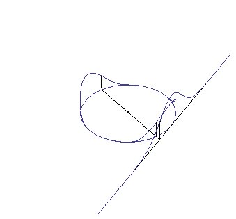
(a)

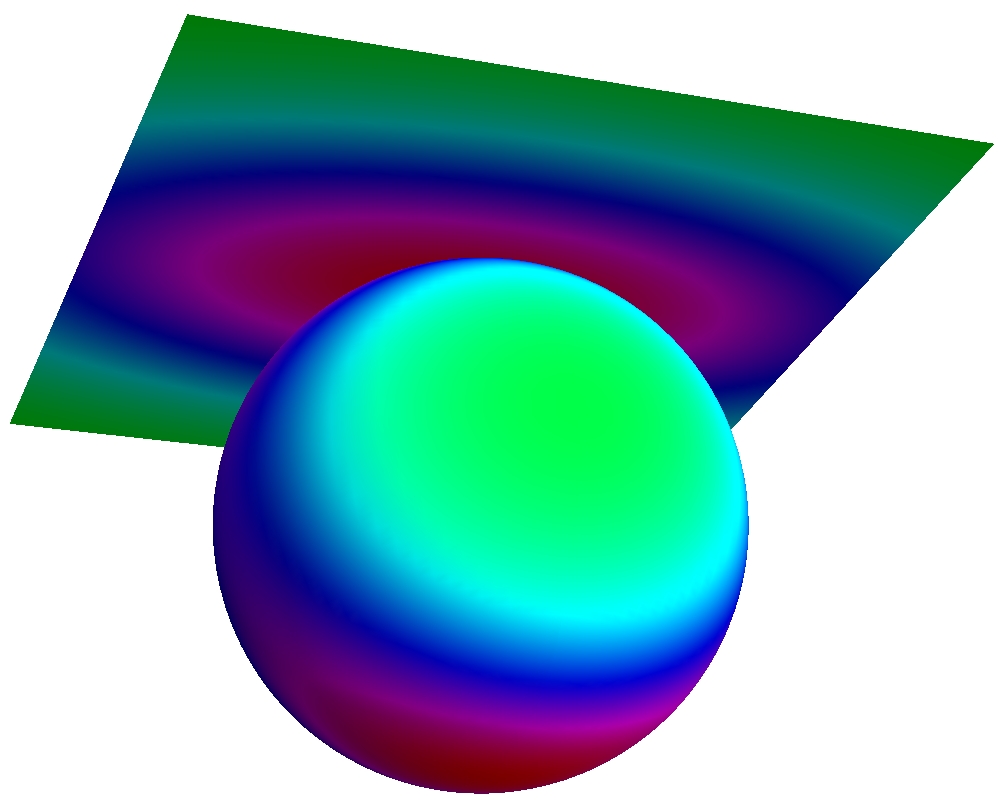
(b)

Figure 1: (a) A base element on the unit circle, obtained by projecting a Gaussian on a tangent line (b) An illustration of a Gaussian distribution projected to a 2D sphere

The subset of $pdfs$ for which $\mu_{u}=\mu_{v}=\mu_{w}=0$ in the corresponding Gaussian on the tangent space is referred to as $PG_{0}$.

Before extending our framework to Mixtures of Projected Gaussians, we would like to explain how to fuse and how to compose two Projected Gaussians.

III-C Fusion and Composition of Projected Gaussians

Two Gaussian distributions $p_{1}\sim\mathcal{N}\left(\mu_{1},\Sigma_{1}\right)$ and $p_{2}\sim\mathcal{N}\left(\mu_{2},\Sigma_{2}\right)$ on $\mathbb{R}^{n}$ pertaining to the same phenomenon are fused by

$$\begin{split}p_{3}&\sim\mathcal{N}\left(\mu_{3},\Sigma_{3}\right)\\ \mu_{3}&=\left(\Sigma_{1}+\Sigma_{2}\right)^{-1}\cdot\left(\Sigma_{1}\cdot\mu_{2}+\Sigma_{2}\cdot\mu_{1}\right)\\ \Sigma_{3}&=\left(\Sigma_{1}^{-1}+\Sigma_{2}^{-1}\right)^{-1}\end{split}$$ (14)

We can generalize this to $PGs$ $p_{1}\sim\mathcal{N}\left(q_{1},\mu_{1},\Sigma_{1}\right)$ and $p_{2}\sim\mathcal{N}\left(q_{2},\mu_{2},\Sigma_{2}\right)$ only if the tangents spaces are reasonably close - the angle between the normals to the tangent spaces should be less than 15^∘, or, equivalently by switching to the antipodal tangent point, larger than 165^∘.

Then we define $q_{3}$ by renormalizing $q_{1}+q_{2}$ to length 1 and restate the original distributions approximately (we show $p_{1}$, $p_{2}$ works the same way). With the Jacobian $J$ at the mean value $\mu_{1}$ of the mapping

$$f=\Pi_{q_{3}}^{-1}\circ\Pi_{q_{1}}:TS_{q_{1}}\longrightarrow TS_{q_{3}}$$ (15)

the parameters are estimated as

$$\mu_{3,1}=f\left(\mu_{1}\right)\;\text{and}\;\Sigma_{3,1}=J\cdot\Sigma_{1}\cdot J^{\top}$$ (16)

Renormalization of the base elements involves an integral that is hard to approximate with quadrature techniques. Therefore we use Monte Carlo integration. Since the integrands are bounded by exponential functions that are easy to sample from, the integration is reasonably efficient.

The estimates resulting from both original distributions are then fused on the common tangent space $TS_{q_{3}}$ using (14). Generally, the rotation part of $\mu_{3}$ is not zero. Since it is advantageous to refrain to base elements of type $PG_{0}$, $p_{3}$ is restated as above with the new tangent point $q_{4}=\Pi_{q_{3}}\left(\mu_{3}\right)$. The resulting probability density function on $S_{3}\times\mathbb{R}^{3}$ needs to be normalized according to Definition 1. The fused $pdf$ is denoted as $p_{3}=\phi\left(p_{1},p_{2}\right)$.

In robotics we frequently need to estimate the $pdf$ of a composition of two subsequent rigid motions given the $pdfs$ of the individual rigid motions (e.g. from an uncertain position in an uncertain camera frame to a position in world coordinates).
Without loss of generality we refrain to $PG_{0}$ to define the composition, so $p_{1}\sim\mathcal{N}\left(q_{1},0,\Sigma_{1}\right)$ and $p_{2}\sim\mathcal{N}\left(q_{2},0,\Sigma_{2}\right)$.

From the composition in terms of dual quaternions $dq_{3}=dq_{2}**\,dq_{1}$ the natural choice for the tangent point $q_{3}$ of the composition is $q_{3}=q_{2}*q_{1}$. This induces a mapping $g$

$$\begin{split}g:&\,TS_{q_{2}}\times TS_{q_{1}}\longrightarrow TS_{q_{3}}\\ g\left(y_{2},y_{1}\right):&=\,\Pi_{q_{3}}^{-1}\left(\Pi_{q_{2}}\left(y_{2}\right)**\,\Pi_{q_{1}}\left(y_{1}\right)\right)\end{split}$$ (17)

Note that $g\left(0,0\right)=0$, thus $\mu_{3}=0$. With

$\left.J_{\gamma}=\frac{\partial g}{\partial\left(y_{2},y_{1}\right)}\right|_{(0,0)}$ and $\Sigma_{\gamma}=\left(\begin{array}[]{cc}\Sigma_{2}&0\\ 0&\Sigma_{1}\end{array}\right)$ the resulting covariance matrix of the composition is $\Sigma_{3}=J_{\gamma}\cdot\Sigma_{C}\cdot J_{\gamma}^{\top}$. The composition $p_{3}\sim\mathcal{N}\left(q_{3},0,\Sigma_{3}\right)$ is denoted by
$p_{3}=\gamma\left(p_{2},p_{1}\right)$.

III-D Mixture of Projected Gaussians $MPG$

As stated above, a precondition for the fusion of $PG$ base elements is that their tangent points are sufficiently close to each other and that they are sufficiently well concentrated. For this reason, widely spread probability density functions should not be modeled in a single base element. Instead, we use a mixture of $PG$ base elements. Thus let $p_{i}\in PG$ be base elements, then a Mixture of Projected Gaussians is defined as

$$p_{m}=\frac{1}{n}\sum_{i=1}^{n}\pi_{i}\cdot p_{i}\quad\text{with}\quad 0\leq\pi_{i}\leq 1\quad\text{and}\quad\sum_{i=1}^{n}\pi_{i}=1$$ (18)

Fusion and composition of $PGs$ carry over to $MPGS$ in a similar way as this work for Mixtures of Gaussians [14].

Let $p_{m,1}=\frac{1}{n}\sum_{i=1}^{n}\pi_{1,i}p_{1,i}$ and $p_{m,2}=\frac{1}{l}\sum_{j=1}^{l}\pi_{2,j}p_{2,j}$ be $MPGS$. The fused mixture $p_{m,3}=\Phi\left(p_{m,1},p_{m,2}\right)$ is obtained by fusing and weighting the base elements of the original mixtures:

$$p_{m,3}=\frac{1}{C}\cdot\sum_{i,j=1}^{n,l}\lambda_{i,j}\cdot\pi_{1,i}\cdot\pi_{2,j}\cdot\phi\left(p_{1,i},p_{2,j}\right)\\$$ (19)

with a normalizing constant

$$C=\sum_{i,j=1}^{n,l}\lambda_{i,j}\cdot\pi_{1,i}\cdot\pi_{2,j}$$ (20)

The weights $\pi_{1,i}$ and $\pi_{2,j}$ are those of the prior mixture. The plausibility is composed of two factors, $\lambda_{i,j}=\alpha_{i,j}\cdot\delta_{i,j}$.

The factor $\alpha$ says whether the mixture elements can share a tangent space and thus probably pertain to the same cases in the mixture (for detail see [2]). The factor $\delta$ is the Mahalanobis distance of the mean values and covariances, transported to the common tangent space.

$$\delta_{i,j}=\mathrm{e}^{-1/2\cdot\left(\mu_{3,1,i}-\mu_{3,2,j}\right)\cdot\left(\Sigma_{3,1,i}+\Sigma_{3,2,j}\right){}^{-1}\cdot\left(\mu_{3,1,i}-\mu_{3,2,j}\right)^{\top}}\\$$

It expresses that even if the mixture elements could share a tangent space, they could still not be compatible.

The composition $p_{m,3}=\Gamma\left(p_{m,1},p_{m,2}\right)$ carries over in a similar manner. In this case, there is no question of whether two base elements could apply at the same time, since the two probability distributions are assumed to be independent, so the factor $\lambda_{i,j}$ is omitted.

$$p_{m,3}=\frac{1}{C}\cdot\sum_{i,j=1}^{n,l}\pi_{1,i}\cdot\pi_{2,j}\cdot\gamma\left(p_{1,i},p_{2,j}\right)$$ (21)

with

$$C=\left(\sum_{i,j=1}^{n,l}\pi_{1,i}\cdot\pi{2,j}\right).$$ (22)

Note that in both cases the individually fused or combined resulting base elements are assumed to be renormalized.

IV $MPG$ and sample based description of $pdfs$

The $MPGs$ try to fill the middle ground between sample based descriptions and unimodal parametric descriptions of $pdfs$. In our perception framework, we use sample based descriptions a lot, so we need to restate $pdfs$ available in one description also in the other one.

Sampling from $MPG$ is easy, we first sample from the discrete $pdf$ induced by the weights, and then draw a sample for the Gaussian on the tangent space using the Box-Muller algorithm.

For fitting a $MPG$ to a sample set, we use a slight variant of the Expectation Maximization Algorithm (see [15]):

1. Set the initial value for the means $\mu_{i}$, covariance matrices $\Sigma_{i}$ and weighting coefficients $\lambda_{i}$ and evaluate the log likelihood with these values.

2. E step:
   Evaluate the responsibilities $\gamma(x_{n,i})$ using the current parameter values

   $$\gamma(z_{j,i}):=\frac{\lambda_{i}\mathcal{N}(x_{j}|TS_{i},\mu_{i},\Sigma_{i})}{\sum_{k}{}{\lambda_{k}\mathcal{N}(x_{j}|TS_{k},\mu_{k},\Sigma_{k})}}$$

3. M step:
   Reestimate the parameters using the current responsibilities

   $$\mu_{i}^{new}=\frac{1}{N_{i}}\sum_{j=1}^{N}{\gamma(z_{j,i})\cdot x_{j}}$$

   $$\Sigma_{i}^{new}=\frac{1}{N_{i}}\sum_{j=1}^{N}{\gamma(z_{j,i})(x_{j}-\mu_{i}^{new})(x_{j}-\mu_{i}^{new})^{\top}}$$

   $$\lambda_{i}^{new}=\frac{N_{i}}{N}$$

   where $N_{i}=\sum_{j=1}^{N}{\gamma(z_{j,i})}$

4. Evaluate the log likelihood:

   $$\ln\mathrm{P}(X|TS,\mu,\Sigma,\lambda)\!=\!\!\sum_{j=1}^{N}{\ln\!\left(\!\sum_{i=1}^{n}{\lambda_{i}\mathcal{N}(x_{j}|TS_{i},\mu_{i},\Sigma_{i})}\!\!\right)}$$

   and check for convergence of either the parameters or the log likelihood. If the convergence criterion is not satisfied return to the E step.
   

Note that we want to keep our base elements in $PG_{0}$, so re-estimating $\mu_{i}$ in the M-Step also means resetting the tangent points $q_{i}$.

V Convergence Properties of the $MPG$

The good news of the $MPG$ framework is that that we get good approximations with few base elements, and that it allows for fusing and composing $pdfs$ without having to go back to the original sensor readings.
The bad news is that the number of base elements tends to increase quadratically with these operations. However, we can drop base elements with small weights and we can merge base elements with similar statistics without loosing much information, while decreasing the number of base elements.

In order to use the framework for the task of grasping, we defined a grasp criterion: Given a $pdf$ $p$ of an object pose and a box $B\subset SE(3)$ that captures the tolerances associated with the grasping task (e.g. width of the gripper, possible grasp on the object), we try to find a rigid transform $m$ that maximizes the probability of successfully grasping:

$$m:=\arg\max_{m\in SE(3)}\int_{m(B)}p(x)d\mu_{m(B)}$$

If $p_{M}(x)=\sum_{i=1}^{n}\lambda_{i}\cdot p(\mu_{i},\Sigma_{i},x)$, the integral is not very much affected by dropping a base element with a small weight, let’s assume the last one. Renormalizing the remaining weights

$$\lambda_{i}^{{}^{\prime}}:=\frac{\lambda_{i}}{1-\lambda_{n}}$$

we get

$$\left|\int\limits_{B}\sum_{i=1}^{n}\lambda_{i}p_{i}\,\mathrm{d}\mu_{B}-\int\limits_{B}\sum_{i=1}^{n-1}\lambda^{\prime}_{i}p_{i}\,\mathrm{d}\mu_{B}\right|<2\lambda_{n}$$

for any box $B$ (for a proof see [2]).

The information loss due to combining two similar base elements is investigated in terms of a symmetric version of the Kullback-Leibler divergence, inspired by an investigation of Runnalls for ordinary mixtures of Gaussians (see [16]). Let’s assume the base elements $p_{1}\sim\mathcal{N}\left(TS_{q_{1}},\mu_{1},\Sigma_{1}\right)$ and $p_{2}\sim\mathcal{N}\left(TS_{q_{2}},\mu_{2},\Sigma_{2}\right)$ from a $MPG$ $M$ have already been restated to the same tangent space, i.e. $q_{1}=q_{2}$. Then the symmetric Kullback-Leibler divergence between them is

$$\begin{split}\mathcal{D}=&(\Sigma_{1}^{-1}+\Sigma_{2}^{-1})(\mu_{1}-\mu_{2})(\mu_{1}-\mu_{2})^{\top}\\ d_{sKL}(p_{1},p_{2})=&\frac{1}{2}\mathrm{tr}\left(\Sigma_{2}^{-1}\Sigma_{1}+\Sigma_{1}^{-1}\Sigma_{2}\quad+\mathcal{D}\right)-6\end{split}$$ (23)

If we now replace both $p_{1}$ and $p_{2}$ with the combined base element

$$p^{\prime}=\frac{1}{\lambda_{1}+\lambda_{2}}\cdot\left(\lambda_{1}p_{1}+\lambda_{2}\cdot p_{2}\right)$$

to obtain the modified $pdf$ $M^{\prime}$ with less base elements, then we have:

$$d_{sKL}(M,M^{\prime})\leq\frac{1}{\lambda_{1}+\lambda_{2}}\cdot\left(\lambda_{1}d_{sKL}(p_{1},p^{\prime})+\lambda_{2}d_{sKL}(p^{\prime},p_{2})\right)$$ (24)

For details and proofs see [2].

VI Implementation and Experimental Results

The $MPG$ framework is fully implemented in Python. The probability density functions are visualized by drawing random samples and for each pose painting a flag on the screen. The foot of the flag represents position, the pole represents the z-axis of the rotated coordinate system, and the tip of the pennant marks the x-axis. As an application example we demonstrate how to estimate the pose of an object based on SIFT features, e.g. the salt box of figure 2. Let’s assume that the robot detects the features ’B’ of the word Bad (green) and ’l’ of Salz (blue). The mountain top will be used as a third feature (purple).

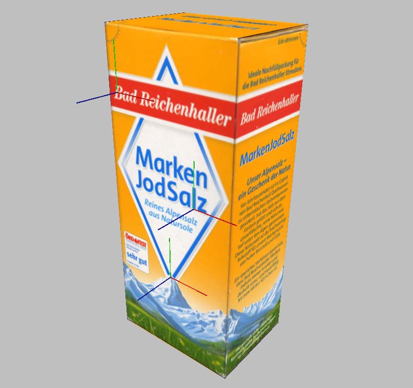
(a)

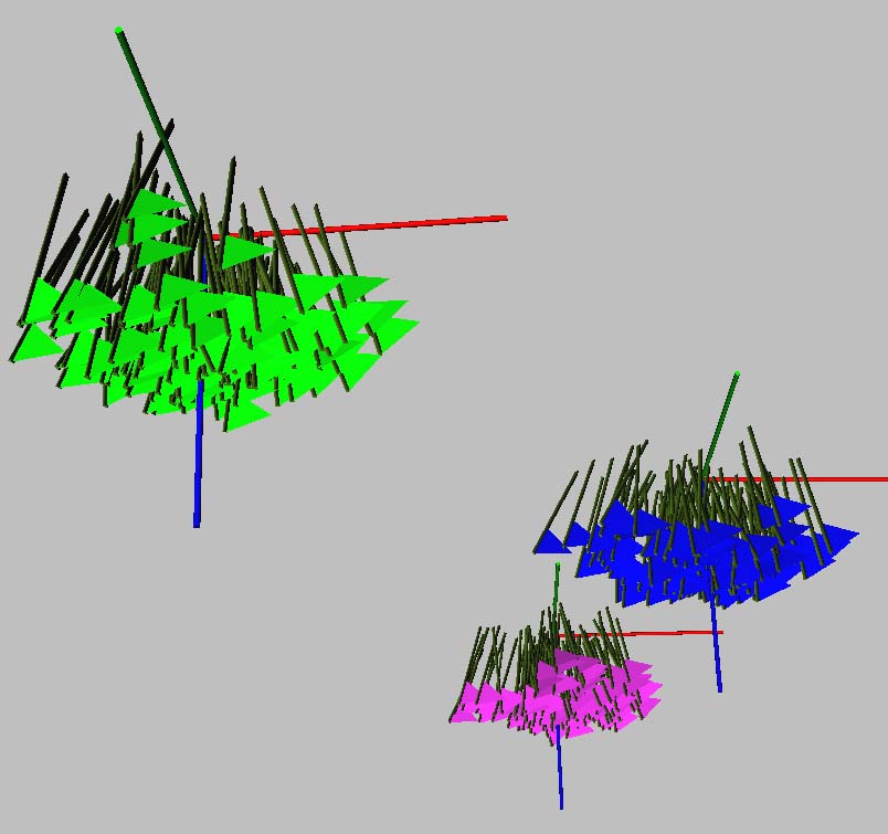
(b)

Figure 2: (a) salt box (b) Stereo SIFT features on the salt box. The features have an orientation around the sight line, but the visibility range is assumed to be $15^{\circ}$, the translation invariance is low. Each feature is represented by a $MPG$ with seven base elements.

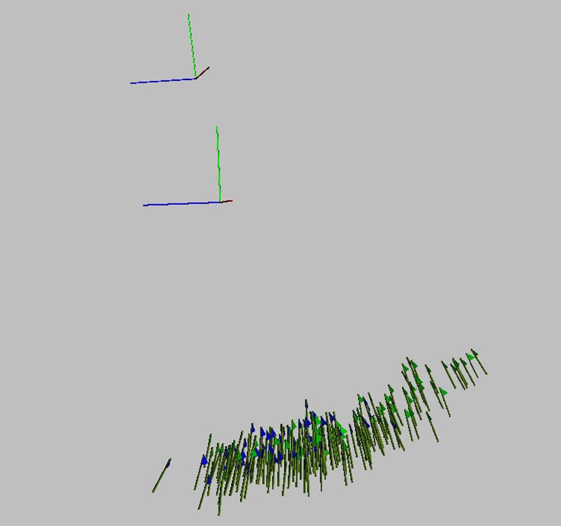
(a)

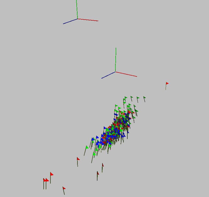
(b)

Figure 3: (a) From the first two SIFT features, two distributions for the object pose are derived by the composition of the rigid motions camera to feature and feature to object coordinate system (b) The two distributions are fused (red).

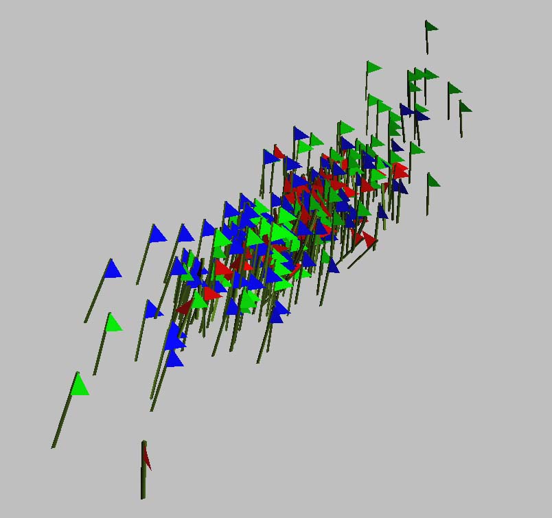
(a)

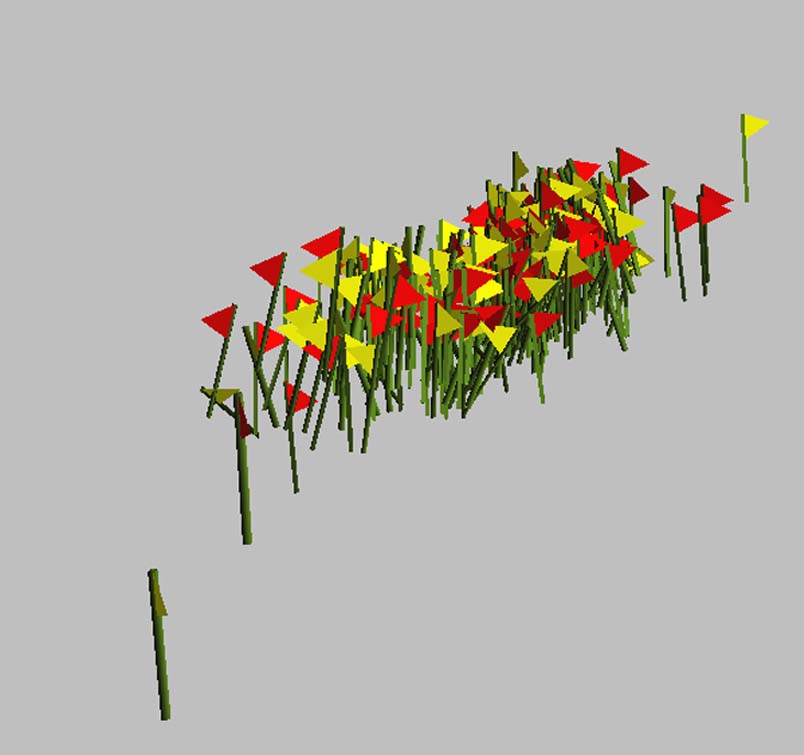
(b)

Figure 4: (a) From originally 49 base elements, ten with low weights are skipped (b) The base elements are merged until only ten are left.

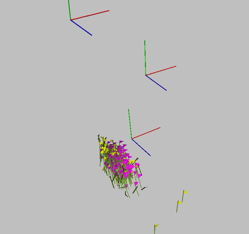
(a)

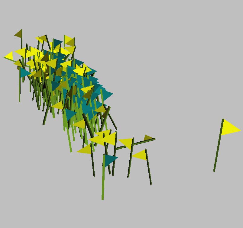
(b)

Figure 5: (a) The object pose estimate from the next feature is added … (b) … and fused with the previous estimate (turquoise).

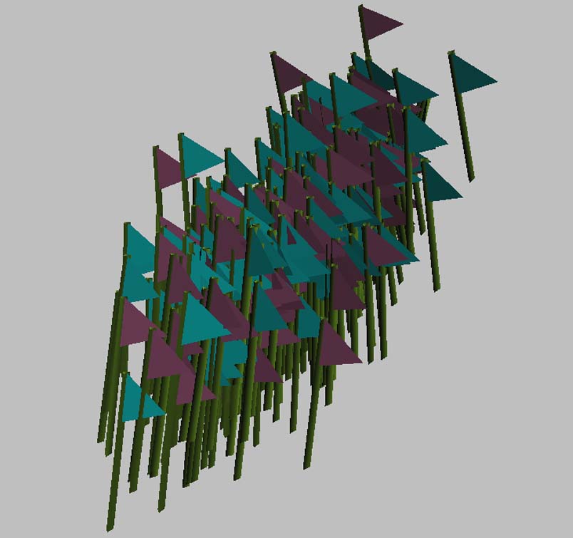
(a)

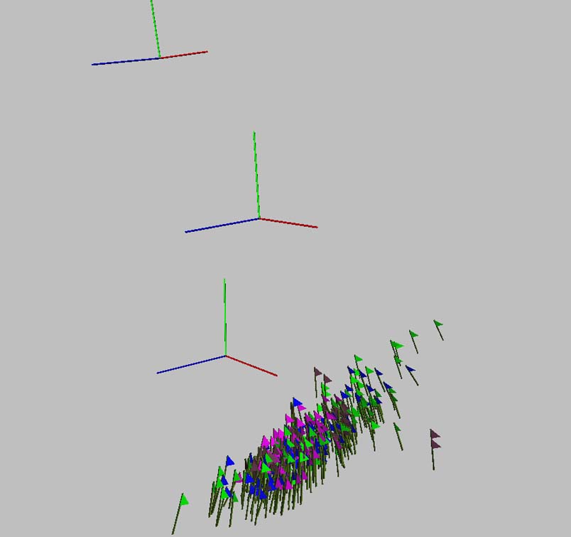
(b)

Figure 6: (a) After merging again, the pose estimate converges. (b) Compare to the original estimates.

VII Conclusion and outlook

In this paper we present the framework of Mixtures of Projected Gaussians that allows for modelling a large variety of possible probability distribution functions of 6D poses. In contrast to a sample based description, much fewer parameters are needed to describe the distribution. The framework interfaces well with the sample based descriptions, and provides the inference mechanisms of fusing and composing uncertain pose information.

The operations of fusion, propagation or multiplication of MPG distributions generally result in a large number of mixture elements. However, many of them have practically zero weight, while others are approximately identical. This is used to drop some base elements, and to merge others, thus reducing their number without losing much information.

The algorithms for probabilistic inference (fusion, propagation, multiplication) are fully implemented in Python.

The covariance matrices are currently estimated using the Jacobian of the non-linear transforms. These estimates could be improved by using the unscented estimation technique (see Julier and Uhlmann [13]).

In this paper we focus on the perception of static objects. The MPG framework can be extended to the dynamic case as well, following concepts by Goddard [6] and by Brox et al. [17].

VIII Acknowledgement

This work was made possible by funding from the ARTEMIS Joint Undertaking as part of the project R3-COP and from the German Federal Ministry of Education and Research (BMBF) under grant no. 01IS10004E.

References

- [1] W. Feiten, P. Atwal, R. Eidenberger, and T. Grundmann, “6D Pose Uncertainty in Robotic Perception,” in Advances in Robotics Research, T. Kröger and F. M. Wahl, Eds. Berlin, Heidelberg: Springer Berlin Heidelberg, 2009, pp. 89–98. [Online]. Available: http://link.springer.com/10.1007/978-3-642-01213-6_9
- [2] M. Lang, “Approximation of Probability Density Functions on the Euclidean Group Parametrized by Dual Quaternions,” arXiv preprint: arXiv:1707.00532, Ludwig-Maximilians-Universität München, 2011. [Online]. Available: https://arxiv.org/abs/1707.00532
- [3] J. Stuelpnagel, “On the Parametrization of the Three-Dimensional Rotation Group,” SIAM Review, vol. 6, no. 4, pp. 422–430, oct 1964. [Online]. Available: http://epubs.siam.org/doi/10.1137/1006093
- [4] S. B. Choe, “Statistical Analysis of Orientation Trajectories via Quaternions with Applications to Human Motion,” no. December, p. 117, 2006.
- [5] J. S. Goddard Jr., “Pose and Motion Estimation from Vision Using Dual Quaternion-based Extended Kalman Filtering,” Ph.D. dissertation, 1997.
- [6] J. S. Goddard and M. A. Abidi, “Pose and Motion Estimation Using Dual quaternion-based Extended Kalman Filtering.” in Image (Rochester, N.Y.), R. N. Ellson and J. H. Nurre, Eds., vol. 3313, no. January, mar 1998, pp. 189–200.
- [7] L. Kavan, S. Collins, C. O’Sullivan, and J. Zara, “Dual quaternions for rigid transformation blending,” Technical report TCDCS200646 Trinity College Dublin, no. TCD-CS-2006-46, pp. 39–48, 2006.
- [8] M. E. Antone and S. Teller, “Robust Camera Pose Recovery Using Stochastic Geometry,” Ph.D. dissertation, 2001.
- [9] J. J. Love, Bingham Statistics. Dordrecht: Springer Netherlands, 2007, pp. 45–47. [Online]. Available: http://dx.doi.org/10.1007/978-1-4020-4423-6_19 http://www.springerlink.com/index/10.1007/978-1-4020-4423-6_19
- [10] J. Glover, G. Bradski, R. R. Rusu, and G. Bradski, “Monte Carlo Pose Estimation with Quaternion Kernels and the Bingham Distribution,” in Robotics: Science and Systems VII. Robotics: Science and Systems Foundation, jun 2011, p. 97.
- [11] K. V. Mardia, C. C. Taylor, and G. K. Subramaniam, “Protein Bioinformatics and Mixtures of Bivariate von Mises Distributions for Angular Data,” Biometrics, vol. 63, no. 2, pp. 505–512, jun 2007. [Online]. Available: http://doi.wiley.com/10.1111/j.1541-0420.2006.00682.x
- [12] E. Kraft, “A quaternion-based unscented Kalman filter for orientation tracking,” in Proceedings of the 6th International Conference on Information Fusion, FUSION 2003, 2003.
- [13] S. J. Julier and J. K. Uhlmann, “A New Extension of the Kalman Filter to Nonlinear Systems,” in Proc. of AeroSense: The 11th Int. Symp. on Aerospace/Defense Sensing, Simulations and Controls, vol. The 11th I, 1997, pp. 182–193.
- [14] R. Eidenberger, T. Grundmann, W. Feiten, and R. Zoellner, “Fast parametric viewpoint estimation for active object detection,” in 2008 IEEE International Conference on Multisensor Fusion and Integration for Intelligent Systems. IEEE, aug 2008, pp. 309–314. [Online]. Available: http://ieeexplore.ieee.org/document/4648083/
- [15] C. M. Bishop, “Pattern Recognition and Machine Learning,” Journal of Electronic Imaging, vol. 16, no. 4, p. 049901, jan 2007.
- [16] A. R. Runnalls, “Kullback-Leibler approach to Gaussian mixture reduction,” IEEE Transactions on Aerospace and Electronic Systems, 2007.
- [17] T. Brox, B. Rosenhahn, U. G. Kersting, and D. Cremers, “Nonparametric Density Estimation for Human Pose Tracking,” in Pattern Recognition, Proceedings, 2006, pp. 546–555. [Online]. Available: http://link.springer.com/10.1007/11861898_55