Graph Convolutional Recurrent Neural Network:
Data-Driven Traffic Forecasting

Abstract

Spatiotemporal forecasting has significant implications in sustainability, transportation and health-care domain. Traffic forecasting is one canonical example of such learning task. This task is challenging due to (1) non-linear temporal dynamics with changing road conditions, (2) complex spatial dependencies on road networks topology and (3) inherent difficulty of long-term time series forecasting. To address these challenges, we propose Graph Convolutional Recurrent Neural Network to incorporate both spatial and temporal dependency in traffic flow. We further integrate the encoder-decoder framework and scheduled sampling to improve long-term forecasting. When evaluated on real-world road network traffic data, our approach can accurately capture spatiotemporal correlations and consistently outperforms state-of-the-art baselines by $12\%$ - $15\%$.

1 Introduction

Spatiotemporal forecasting is a crucial task for a learning system that operates in a dynamic environment. It has a wide range of applications from autonomous vehicles operations, to energy and smart grid optimization, to logistics and supply chain management. In this paper, we study one important task: traffic forecasting on road networks, the core component of the intelligent transportation systems. The goal of traffic forecasting is to predict the future traffic speeds of a sensor network given historic traffic speeds and the underlying road networks.

Figure 1: Spatial correlation is dominated by road network structure. (1) Traffic speed in road 1 are similar to road 2 as they locate in the same highway. (2) Road 1 and road 3 locate in the opposite directions of the highway. Though close to each other in the Euclidean space, their road network distance is large, and their traffic speeds differ significantly.

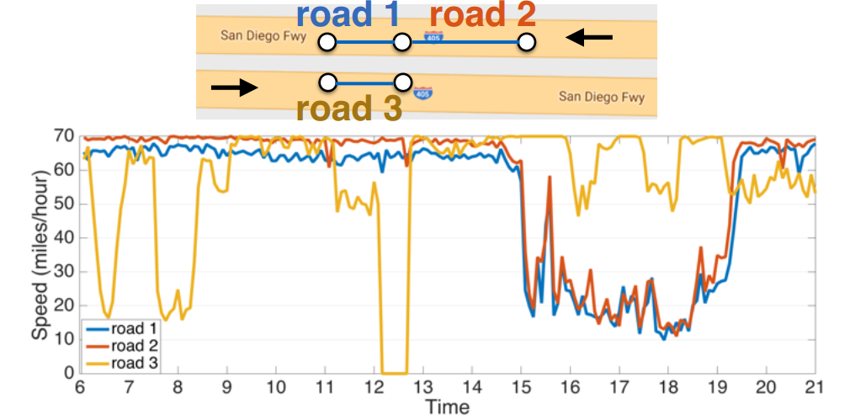
This task is challenging mainly due to the complex spatiotemporal dependencies and inherent difficulty in the long term forecasting. On the one hand, traffic time series demonstrate strong temporal dynamics. Recurring incidents such as rush hours or accidents can cause non-stationarity, making it difficult to forecast long-term. On the other hand, sensors on the road network contain complex yet unique spatial correlations. Figure 1 illustrates an example. Road $1$ and road $2$ are correlated, while road $1$ and road $3$ are not. Although road $1$ and road $3$ are close in the Euclidean space, they demonstrate very different behaviors. Moreover, the future traffic speed is influenced more by the downstream traffic than the upstream one. This means that the spatial structure in traffic is non-Euclidean and directional.

Traffic forecasting has been studied for decades, falling into two main categories: knowledge-driven approach and data-driven approach. In transportation and operational research, knowledge-driven methods usually apply queuing theory and simulate user behaviors in traffic (cascetta2013transportation). In time series community, data-driven methods such as Auto-Regressive Integrated Moving Average (ARIMA) model and Kalman filtering remain popular (liu2011discovering; lippi2013short). However, simple time series models usually rely on the stationarity assumption, which is often violated by the traffic data. Most recently, deep learning models for traffic forecasting have been developed in lv2015traffic; deeptraffic2017, but without considering the spatial structure. wu2016short and ma2017learning model the spatial correlation with Convolutional Neural Networks (CNN), but the spatial structure is in the Euclidean space (e.g., 2D images).  bruna2013spectral, defferrard2016convolutional studied graph convolution, but only for undirected graphs.

In this work, we represent the pair-wise spatial correlations between traffic sensors using a directed graph whose nodes are sensors and edge weights denote proximity between the sensor pairs measured by the road network distance. We model the dynamics of the traffic flow as a diffusion process and propose the diffusion convolution operation to capture the spatial dependency. We further propose Diffusion Convolutional Recurrent Neural Network (DCRNN) that integrates diffusion convolution, the sequence to sequence architecture and the scheduled sampling technique. When evaluated on real-world traffic datasets, DCRNN consistently outperforms state-of-the-art traffic forecasting baselines by a large margin. In summary:

• We study the traffic forecasting problem and model the spatial dependency of traffic as a diffusion process on a directed graph. We propose diffusion convolution, which has an intuitive interpretation and can be computed efficiently.

• We propose Diffusion Convolutional Recurrent Neural Network (DCRNN), a holistic approach that captures both spatial and temporal dependencies among time series using diffusion convolution and the sequence to sequence learning framework together with scheduled sampling. DCRNN is not limited to transportation and is readily applicable to other spatiotemporal forecasting tasks.

• We conducted extensive experiments on two large-scale real-world datasets, and the proposed approach obtains significant improvement over state-of-the-art baseline methods.

2 Related Work

Traffic forecasting is a classic problem in transportation and operational research which are primarily based on queuing theory and simulations (drew1968traffic). Data-driven approaches for traffic forecasting have received considerable attention, and more details can be found in a recent survey paper (vlahogianni2014short) and the references therein. However, existing machine learning models either impose strong stationary assumptions on the data (e.g., auto-regressive model) or fail to account for highly non-linear temporal dependency (e.g., latent space model yu2016temporal; DengSDZYL16). Deep learning models deliver new promise for time series forecasting problem. For example, in deeptraffic2017; laptev2017time, the authors study time series forecasting using deep Recurrent Neural Networks (RNN). Convolutional Neural Networks (CNN) have also been applied to traffic forecasting. zhang2016dnn; zhang2017deep convert the road network to a regular 2-D grid and apply traditional CNN to predict crowd flow. cheng2017deeptransport propose DeepTransport which models the spatial dependency by explicitly collecting upstream and downstream neighborhood roads for each individual road and then conduct convolution on these neighborhoods respectively.

Recently, CNN has been generalized to arbitrary graphs based on the spectral graph theory. Graph convolutional neural networks (GCN) are first introduced in  bruna2013spectral, which bridges the spectral graph theory and deep neural networks. defferrard2016convolutional propose ChebNet which improves GCN with fast localized convolutions filters. kipf2016semi simplify ChebNet and achieve state-of-the-art performance in semi-supervised classification tasks. seo2016structured combine ChebNet with Recurrent Neural Networks (RNN) for structured sequence modeling.  yu2017spatio model the sensor network as a undirected graph and applied ChebNet and convolutional sequence model (gehring2017convolutional) to do forecasting. One limitation of the mentioned spectral based convolutions is that they generally require the graph to be undirected to calculate meaningful spectral decomposition. Going from spectral domain to vertex domain, atwood2016diffusion propose diffusion-convolutional neural network (DCNN) which defines convolution as a diffusion process across each node in a graph-structured input. hechtlinger2017generalization propose GraphCNN to generalize convolution to graph by convolving every node with its $p$ nearest neighbors. However, both these methods do not consider the temporal dynamics and mainly deal with static graph settings.

Our approach is different from all those methods due to both the problem settings and the formulation of the convolution on the graph. We model the sensor network as a weighted directed graph which is more realistic than grid or undirected graph. Besides, the proposed convolution is defined using bidirectional graph random walk and is further integrated with the sequence to sequence learning framework as well as the scheduled sampling to model the long-term temporal dependency.

3 Methodology

We formalize the learning problem of spatiotemporal traffic forecasting and describe how to model the dependency structures using diffusion convolutional recurrent neural network.

3.1 Traffic Forecasting Problem

The goal of traffic forecasting is to predict the future traffic speed given previously observed traffic flow from $N$ correlated sensors on the road network. We can represent the sensor network as a weighted directed graph $\mathcal{G}=(\mathcal{V},\mathcal{E},{{\bm{W}}})$, where $\mathcal{V}$ is a set of nodes ${\left|\mathcal{V}\right|}=N$, $\mathcal{E}$ is a set of edges and ${{\bm{W}}}{}\in{}^{N\times N}$ is a weighted adjacency matrix representing the nodes proximity (e.g., a function of their road network distance). Denote the traffic flow observed on $\mathcal{G}$ as a graph signal ${\bm{X}}\in{}^{N\times P}$, where $P$ is the number of features of each node (e.g., velocity, volume). Let ${\bm{X}}^{(t)}$ represent the graph signal observed at time $t$, the traffic forecasting problem aims to learn a function $h(\cdot)$ that maps $T^{\prime}$ historical graph signals to future $T$ graph signals, given a graph $\mathcal{G}$:

$$[{\bm{X}}^{(t-T^{\prime}+1)},\cdots,{\bm{X}}^{(t)};\mathcal{G}]\xrightarrow[]{h(\cdot)}[{\bm{X}}^{(t+1)},\cdots,{\bm{X}}^{(t+T)}]$$

3.2 Spatial Dependency Modeling

We model the spatial dependency by relating traffic flow to a diffusion process, which explicitly captures the stochastic nature of traffic dynamics. This diffusion process is characterized by a random walk on $\mathcal{G}$ with restart probability $\alpha\in[0,1]$, and a state transition matrix ${\bm{D}}_{O}^{-1}{\bm{W}}$. Here ${\bm{D_{O}}}=\mathrm{diag}({\bm{W}}{\bm{1}})$ is the out-degree diagonal matrix, and ${\bm{1}}\in{}^{N}$ denotes the all one vector. After many time steps, such Markov process converges to a stationary distribution ${\bm{{\mathcal{P}}}}\in{}^{N\times N}$ whose $i$th row ${\bm{{\mathcal{P}}}}_{i,:}\in\real{}^{N}$ represents the likelihood of diffusion from node $v_{i}\in\mathcal{V}$, hence the proximity w.r.t. the node $v_{i}$. The following Lemma provides a closed form solution for the stationary distribution.

Lemma 3.1

(teng2016scalable) The stationary distribution of the diffusion process can be represented as a weighted combination of infinite random walks on the graph, and be calculated in closed form:

$${\bm{{\mathcal{P}}}}=\sum_{k=0}^{\infty}\alpha(1-\alpha)^{k}\left({\bm{D}}_{O}^{-1}{\bm{W}}\right)^{k}$$ (1)

where $k$ is the diffusion step. In practice, we use a finite $K$-step truncation of the diffusion process and assign a trainable weight to each step. We also include the reversed direction diffusion process, such that the bidirectional diffusion offers the model more flexibility to capture the influence from both the upstream and the downstream traffic.

Diffusion Convolution

The resulted diffusion convolution operation over a graph signal ${\bm{X}}\in{}^{N\times P}$ and a filter $f_{\bm{\theta}}$ is defined as:

$${\bm{X}}_{:,p}{\,\star_{\mathcal{G}}\,}{}f_{\bm{\theta}}=\sum_{k=0}^{K-1}\left(\theta_{k,1}\left({\bm{D}}_{O}^{-1}{\bm{W}}\right)^{k}+\theta_{k,2}\left({\bm{D}}_{I}^{-1}{\bm{W}}^{\intercal}\right)^{k}\right){\bm{X}}_{:,p}\quad\text{for }p\in\{1,\cdots,P\}$$ (2)

where ${\bm{\theta}}\in{}^{K\times 2}$ are the parameters for the filter and ${\bm{D}}_{O}^{-1}{\bm{W}},{\bm{D}}_{I}^{-1}{\bm{W}}^{\intercal}$ represent the transition matrices of the diffusion process and the reverse one, respectively. In general, computing the convolution can be expensive. However, if $\mathcal{G}$ is sparse, Equation 2 can be calculated efficiently using $O(K)$ recursive sparse-dense matrix multiplication with total time complexity $O(K|\mathcal{E}|)\ll O(N^{2})$. See Appendix LABEL:sec:recursive_calculation for more detail.

Diffusion Convolutional Layer

With the convolution operation defined in Equation 2, we can build a diffusion convolutional layer that maps $P$-dimensional features to $Q$-dimensional outputs. Denote the parameter tensor as ${\bm{{{\mathbf{\mathsf{\Theta}}}}}}\in{}^{Q\times P\times K\times 2}=[{\bm{\theta}}]_{q,p}$, where ${\bm{{\Theta}}}_{q,p,:,:}\in{}^{K\times 2}$ parameterizes the convolutional filter for the $p$th input and the $q$th output. The diffusion convolutional layer is thus:

$${\bm{H}}_{:,q}={\bm{a}}\left(\sum_{p=1}^{P}{\bm{X}}_{:,p}{\,\star_{\mathcal{G}}\,}{}f_{{\bm{{{\mathbf{\mathsf{\Theta}}}}}}_{q,p,:,:}}\right)\qquad\text{for}\;q\in\{1,\cdots,Q\}$$ (3)

where ${\bm{X}}\in{}^{N\times P}$ is the input, ${\bm{H}}\in{}^{N\times Q}$ is the output, $\{f_{{\bm{{{\mathbf{\mathsf{\Theta}}}}}}_{q,p,,:}}\}$ are the filters and ${\bm{a}}$ is the activation function (e.g., ReLU, Sigmoid). Diffusion convolutional layer learns the representations for graph structured data and we can train it using stochastic gradient based method.

Relation with Spectral Graph Convolution

Diffusion convolution is defined on both directed and undirected graphs. When applied to undirected graphs, we show that many existing graph structured convolutional operations including the popular spectral graph convolution, i.e., ChebNet (defferrard2016convolutional), can be considered as a special case of diffusion convolution (up to a similarity transformation). Let ${\bm{D}}$ denote the degree matrix, and ${\bm{L}}={\bm{D}}^{-\frac{1}{2}}({\bm{D}}-{\bm{W}}){\bm{D}}^{-\frac{1}{2}}$ be the normalized graph Laplacian, the following Proposition demonstrates the connection.

Proposition 3.2

The spectral graph convolution defined as

$${\bm{X}}_{:,p}{\,\star_{\mathcal{G}}\,}{}f_{\bm{\theta}}={\bm{\Phi}}\;F({\bm{\theta}})\;{\bm{\Phi}}^{\intercal}{\bm{X}}_{:,p}$$

with eigenvalue decomposition ${\bm{L}}=\mathbf{\Phi}\Lambda\mathbf{\Phi}^{\intercal}$ and $F({\bm{\theta}})=\sum_{0}^{K-1}\theta_{k}{\bm{\Lambda}}^{k}$, is equivalent to graph diffusion convolution up to a similarity transformation, when the graph $\mathcal{G}$ is undirected.

See Appendix LABEL:sec:gconv_relationship.

Figure 2: System architecture for the Diffusion Convolutional Recurrent Neural Network designed for spatiotemporal traffic forecasting. The historical time series are fed into an encoder whose final states are used to initialize the decoder. The decoder makes predictions based on either previous ground truth or the model output.

3.3 Temporal Dynamics Modeling

We leverage the recurrent neural networks (RNNs) to model the temporal dependency. In particular, we use Gated Recurrent Units (GRU) (chung2014empirical), which is a simple yet powerful variant of RNNs. We replace the matrix multiplications in GRU with the diffusion convolution, which leads to our proposed Diffusion Convolutional Gated Recurrent Unit (DCGRU).

$${\bm{r}}^{(t)}= \sigma({\bm{\Theta}}_{r}{\,\star_{\mathcal{G}}\,}{}[{\bm{X}}^{(t)},\;{\bm{H}}^{(t-1)}]+{\bm{b}}_{r})\; {\bm{u}}^{(t)}=\sigma({\bm{\Theta}}_{u}{\,\star_{\mathcal{G}}\,}{}[{\bm{X}}^{(t)},\;{\bm{H}}^{(t-1)}]+{\bm{b}}_{u})$$

$${\bm{C}}^{(t)}= \tanh({\bm{\Theta}}_{C}{\,\star_{\mathcal{G}}\,}{}\left[{\bm{X}}^{(t)},\;({\bm{r}}^{(t)}\odot{\bm{H}}^{(t-1)})\right]+{\bm{b}}_{c})\; {\bm{H}}^{(t)}={\bm{u}}^{(t)}\odot{}{\bm{H}}^{(t-1)}+(1-{\bm{u}}^{(t)})\odot{}{\bm{C}}^{(t)}$$

where ${\bm{X}}^{(t)},{\bm{H}}^{(t)}$ denote the input and output of at time $t$, ${\bm{r}}^{(t)},{\bm{u}}^{(t)}$ are reset gate and update gate at time $t$, respectively. ${\,\star_{\mathcal{G}}\,}{}$ denotes the diffusion convolution defined in Equation 2 and ${\bm{\Theta}}_{r},{\bm{\Theta}}_{u},{\bm{\Theta}}_{C}$ are parameters for the corresponding filters. Similar to GRU, DCGRU can be used to build recurrent neural network layers and be trained using backpropagation through time.

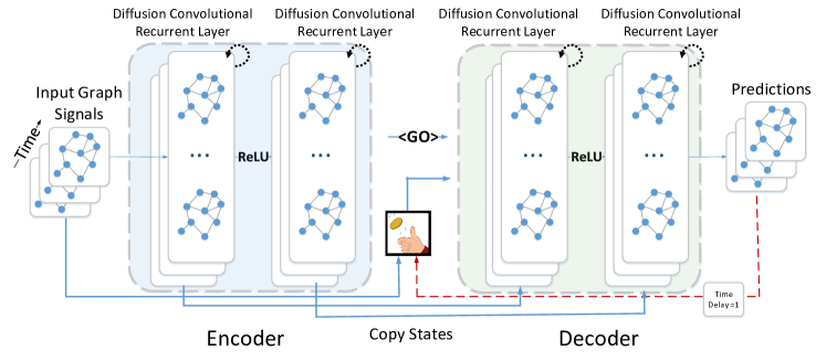
In multiple step ahead forecasting, we employ the Sequence to Sequence architecture (sutskever2014sequence). Both the encoder and the decoder are recurrent neural networks with DCGRU. During training, we feed the historical time series into the encoder and use its final states to initialize the decoder. The decoder generates predictions given previous ground truth observations. At testing time, ground truth observations are replaced by predictions generated by the model itself. The discrepancy between the input distributions of training and testing can cause degraded performance. To mitigate this issue, we integrate scheduled sampling (bengio2015scheduled) into the model, where we feed the model with either the ground truth observation with probability $\epsilon_{i}$ or the prediction by the model with probability $1-\epsilon_{i}$ at the $i$th iteration. During the training process, $\epsilon_{i}$ gradually decreases to $0$ to allow the model to learn the testing distribution.

With both spatial and temporal modeling, we build a Diffusion Convolutional Recurrent Neural Network (DCRNN). The model architecture of DCRNN is shown in Figure  2. The entire network is trained by maximizing the likelihood of generating the target future time series using backpropagation through time. DCRNN is able to capture spatiotemporal dependencies among time series and can be applied to various spatiotemporal forecasting problems.

4 Experiments

We conduct experiments on two real-world large-scale datasets: (1) METR-LA This traffic dataset contains traffic information collected from loop detectors in the highway of Los Angeles County (Jagadish2014). We select 207 sensors and collect 4 months of data ranging from Mar 1st 2012 to Jun 30th 2012 for the experiment. (2) PEMS-BAY This traffic dataset is collected by California Transportation Agencies (CalTrans) Performance Measurement System (PeMS). We select 325 sensors in the Bay Area and collect 6 months of data ranging from Jan 1st 2017 to May 31th 2017 for the experiment. The sensor distributions of both datasets are visualized in  Figure LABEL:fig:sensor_distribution in the Appendix.

In both of those datasets, we aggregate traffic speed readings into 5 minutes windows, and apply Z-Score normalization. 70% of data is used for training, 20% are used for testing while the remaining 10% for validation. To construct the sensor graph, we compute the pairwise road network distances between sensors and build the adjacency matrix using thresholded Gaussian kernel (shuman2013emerging). $W_{ij}=\exp{\left(-\frac{\mathrm{dist}({v_{i},v_{j}})^{2}}{\sigma^{2}}\right)}\quad\text{if }\mathrm{dist}(v_{i},v_{j})\leq\kappa\text{, otherwise }0,$ where $W_{ij}$ represents the edge weight between sensor $v_{i}$ and sensor $v_{j}$, $\mathrm{dist}({v_{i},v_{j}})$ denotes the road network distance from sensor $v_{i}$ to sensor $v_{j}$. $\sigma$ is the standard deviation of distances and $\kappa$ is the threshold.

4.1 Experimental Settings

Baselines

Table 1: Performance comparison of different approaches for traffic speed forecasting. DCRNN achieves the best performance with all three metrics for all forecasting horizons, and the advantage becomes more evident with the increase of the forecasting horizon.

	$T$	Metric	HA	ARIMAKal	VAR	SVR	FNN	FC-LSTM	DCRNN
METR-LA	15 min	MAE	4.16	3.99	4.42	3.99	3.99	3.44	2.77
		RMSE	7.80	8.21	7.89	8.45	7.94	6.30	5.38
		MAPE	13.0%	9.6%	10.2%	9.3%	9.9%	9.6%	7.3%
	30 min	MAE	4.16	5.15	5.41	5.05	4.23	3.77	3.15
		RMSE	7.80	10.45	9.13	10.87	8.17	7.23	6.45
		MAPE	13.0%	12.7%	12.7%	12.1%	12.9%	10.9%	8.8%
	1 hour	MAE	4.16	6.90	6.52	6.72	4.49	4.37	3.60
		RMSE	7.80	13.23	10.11	13.76	8.69	8.69	7.59
		MAPE	13.0%	17.4%	15.8%	16.7%	14.0%	13.2%	10.5%
PEMS-BAY	15 min	MAE	2.88	1.62	1.74	1.85	2.20	2.05	1.38
		RMSE	5.59	3.30	3.16	3.59	4.42	4.19	2.95
		MAPE	6.8%	3.5%	3.6%	3.8%	5.19%	4.8%	2.9%
	30 min	MAE	2.88	2.33	2.32	2.48	2.30	2.20	1.74
		RMSE	5.59	4.76	4.25	5.18	4.63	4.55	3.97
		MAPE	6.8%	5.4%	5.0%	5.5%	5.43%	5.2%	3.9%
	1 hour	MAE	2.88	3.38	2.93	3.28	2.46	2.37	2.07
		RMSE	5.59	6.50	5.44	7.08	4.98	4.96	4.74
		MAPE	6.8%	8.3%	6.5%	8.0%	5.89%	5.7%	4.9%

We compare DCRNN with widely used time series regression models, including (1) HA: Historical Average, which models the traffic flow as a seasonal process, and uses weighted average of previous seasons as the prediction; (2) ARIMA_kal: Auto-Regressive Integrated Moving Average model with Kalman filter which is widely used in time series prediction; (3) VAR: Vector Auto-Regression (hamilton1994time). (4) SVR: Support Vector Regression which uses linear support vector machine for the regression task; The following deep neural network based approaches are also included: (5) Feed forward Neural network (FNN): Feed forward neural network with two hidden layers and L2 regularization. (6) Recurrent Neural Network with fully connected LSTM hidden units (FC-LSTM) (sutskever2014sequence).

All neural network based approaches are implemented using Tensorflow (abadi2016tensorflow), and trained using the Adam optimizer with learning rate annealing. The best hyperparameters are chosen using the Tree-structured Parzen Estimator (TPE) (bergstra2011algorithms) on the validation dataset. Detailed parameter settings for DCRNN as well as baselines are available in Appendix LABEL:sec:detailed_exp_settings.

4.2 Traffic Forecasting Performance Comparison

Table 1 shows the comparison of different approaches for 15 minutes, 30 minutes and 1 hour ahead forecasting on both datasets. These methods are evaluated based on three commonly used metrics in traffic forecasting, including (1) Mean Absolute Error (MAE), (2) Mean Absolute Percentage Error (MAPE), and (3) Root Mean Squared Error (RMSE). Missing values are excluded in calculating these metrics. Detailed formulations of these metrics are provided in Appendix LABEL:sec:metrics. We observe the following phenomenon in both of these datasets. (1) RNN-based methods, including FC-LSTM and DCRNN, generally outperform other baselines which emphasizes the importance of modeling the temporal dependency. (2) DCRNN achieves the best performance regarding all the metrics for all forecasting horizons, which suggests the effectiveness of spatiotemporal dependency modeling. (3) Deep neural network based methods including FNN, FC-LSTM and DCRNN, tend to have better performance than linear baselines for long-term forecasting, e.g., 1 hour ahead. This is because the temporal dependency becomes increasingly non-linear with the growth of the horizon. Besides, as the historical average method does not depend on short-term data, its performance is invariant to the small increases in the forecasting horizon.

Note that, traffic forecasting on the METR-LA (Los Angeles, which is known for its complicated traffic conditions) dataset is more challenging than that in the PEMS-BAY (Bay Area) dataset. Thus we use METR-LA as the default dataset for following experiments.

4.3 Effect of spatial dependency modeling

Figure 3: Learning curve for DCRNN and DCRNN without diffusion convolution. Removing diffusion convolution results in much higher validation error. Moreover, DCRNN with bi-directional random walk achieves the lowest validation error.

Figure 4: Effects of K and the number of units in each layer of DCRNN. K corresponds to the reception field width of the filter, and the number of units corresponds to the number of filters.

Table 2: Performance comparison for DCRNN and GCRNN on the METRA-LA dataset.

	15 min			30 min			1 hour
	MAE	RMSE	MAPE	MAE	RMSE	MAPE	MAE	RMSE	MAPE
DCRNN	2.77	5.38	7.3%	3.15	6.45	8.8%	3.60	7.60	10.5%
GCRNN	2.80	5.51	7.5%	3.24	6.74	9.0%	3.81	8.16	10.9%

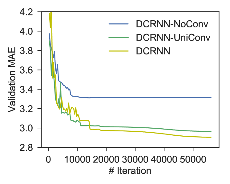
To further investigate the effect of spatial dependency modeling, we compare DCRNN with the following variants: (1) DCRNN-NoConv, which ignores spatial dependency by replacing the transition matrices in the diffusion convolution (Equation 2) with identity matrices. This essentially means the forecasting of a sensor can be only be inferred from its own historical readings; (2) DCRNN-UniConv, which only uses the forward random walk transition matrix for diffusion convolution; Figure 4 shows the learning curves of these three models with roughly the same number of parameters. Without diffusion convolution, DCRNN-NoConv has much higher validation error. Moreover, DCRNN achieves the lowest validation error which shows the effectiveness of using bidirectional random walk. The intuition is that the bidirectional random walk gives the model the ability and flexibility to capture the influence from both the upstream and the downstream traffic.

To investigate the effect of graph construction, we construct a undirected graph by setting $\widehat{W}_{ij}=\widehat{W}_{ji}=\max(W_{ij},W_{ji})$, where $\widehat{{\bm{W}}}$ is the new symmetric weight matrix. Then we develop a variant of DCRNN denotes GCRNN, which uses the sequence to sequence learning with ChebNet graph convolution (Equation LABEL:eq:chebnet) with roughly the same amount of parameters. Table 2 shows the comparison between DCRNN and GCRNN in the METR-LA dataset. DCRNN consistently outperforms GCRNN. The intuition is that directed graph better captures the asymmetric correlation between traffic sensors.

Figure 5: Performance comparison for different DCRNN variants. DCRNN, with the sequence to sequence framework and scheduled sampling, achieves the lowest MAE on the validation dataset. The advantage becomes more clear with the increase of the forecasting horizon.

Figure 6: Traffic time series forecasting visualization. DCRNN generates smooth prediction and is usually better at predict the start and end of peak hours.

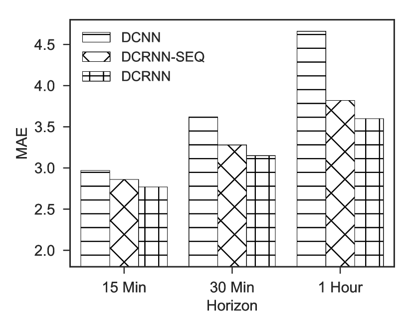
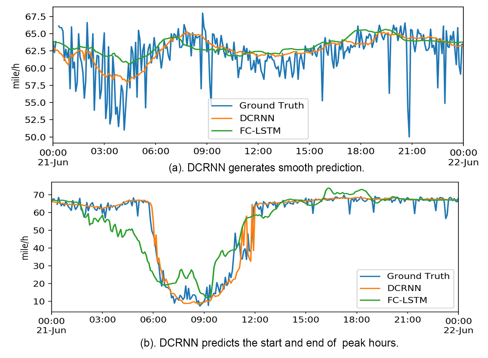
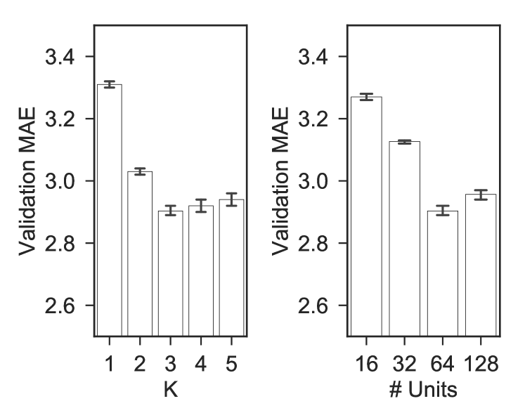
Figure 4 shows the effects of different parameters. $K$ roughly corresponds to the size of filters’ reception fields while the number of units corresponds to the number of filters. Larger $K$ enables the model to capture broader spatial dependency at the cost of increasing learning complexity. We observe that with the increase of $K$, the error on the validation dataset first quickly decrease, and then slightly increase. Similar behavior is observed for varying the number of units.

4.4 Effect of temporal dependency modeling

To evaluate the effect of temporal modeling including the sequence to sequence framework as well as the scheduled sampling mechanism, we further design three variants of DCRNN: (1) DCNN: in which we concatenate the historical observations as a fixed length vector and feed it into stacked diffusion convolutional layers to predict the future time series. We train a single model for one step ahead prediction, and feed the previous prediction into the model as input to perform multiple steps ahead prediction. (2) DCRNN-SEQ: which uses the encoder-decoder sequence to sequence learning framework to perform multiple steps ahead forecasting. (3) DCRNN: similar to DCRNN-SEQ except for adding scheduled sampling.

Figure 6 shows the comparison of those four methods with regards to MAE for different forecasting horizons. We observe that: (1) DCRNN-SEQ outperforms DCNN by a large margin which conforms the importance of modeling temporal dependency. (2) DCRNN achieves the best result, and its superiority becomes more evident with the increase of the forecasting horizon. This is mainly because the model is trained to deal with its mistakes during multiple steps ahead prediction and thus suffers less from the problem of error propagation. We also train a model that always been fed its output as input for multiple steps ahead prediction. However, its performance is much worse than all the three variants which emphasizes the importance of scheduled sampling.

4.5 Model Interpretation

Figure 7: Visualization of learned localized filters centered at different nodes with $K=3$ on the METR-LA dataset. The star denotes the center, and the colors represent the weights. We observe that weights are localized around the center, and diffuse alongside the road network.

To better understand the model, we visualize forecasting results as well as learned filters. Figure 6 shows the visualization of 1 hour ahead forecasting. We have the following observations: (1) DCRNN generates smooth prediction of the mean when small oscillation exists in the traffic speeds (Figure 6(a)). This reflects the robustness of the model. (2) DCRNN is more likely to accurately predict abrupt changes in the traffic speed than baseline methods (e.g., FC-LSTM). As shown in Figure 6(b), DCRNN predicts the start and the end of the peak hours. This is because DCRNN captures the spatial dependency, and is able to utilize the speed changes in neighborhood sensors for more accurate forecasting. Figure 7 visualizes examples of learned filters centered at different nodes. The star denotes the center, and colors denote the weights. We can observe that (1) weights are well localized around the center, and (2) the weights diffuse based on road network distance. More visualizations are provided in Appendix LABEL:sec:model_visualization.

5 Conclusion

In this paper, we formulated the traffic prediction on road network as a spatiotemporal forecasting problem, and proposed the diffusion convolutional recurrent neural network that captures the spatiotemporal dependencies. Specifically, we use bidirectional graph random walk to model spatial dependency and recurrent neural network to capture the temporal dynamics. We further integrated the encoder-decoder architecture and the scheduled sampling technique to improve the performance for long-term forecasting. When evaluated on two large-scale real-world traffic datasets, our approach obtained significantly better prediction than baselines. For future work, we will investigate the following two aspects (1) applying the proposed model to other spatial-temporal forecasting tasks; (2) modeling the spatiotemporal dependency when the underlying graph structure is evolving, e.g., the K nearest neighbor graph for moving objects.