Detecting topological transitions in two dimensions by Hamiltonian evolution

Abstract

We show that the evolution of two-component particles governed by a two-dimensional spin-orbit lattice Hamiltonian can reveal transitions between topological phases. A kink in the mean width of the particle distribution signals the closing of the band gap, a prerequisite for a quantum phase transition between topological phases. Furthermore, for realistic and experimentally motivated Hamiltonians the density profile in topologically non-trivial phases displays characteristic rings in the vicinity of the origin that are absent in trivial phases. The results are expected to have immediate application to systems of ultracold atoms and photonic lattices.

Topological phases have many unusual and potentially useful electronic properties, and have been proposed for fault-tolerant quantum computation and quantum memories Moore2010 ; Hasan2010 ; Ryu2010 ; Qi2011 ; Pachos2014 . In one dimensional systems, all topological states can be classified Chen2011 . In higher dimensions, non-interacting systems can be classified in terms of topological invariants such as Chern numbers Chiu2016 , and much work has been expended in recent years attempting to extend this classification to interacting systems Chen2012 ; Wang2014 ; Wang2015a ; Wang2015b . The experimental determination of topological invariants in bulk condensed matter systems with time-reversal symmetry is not straightforward, however; topological order would generally be inferred from the existence of edge states Hasan2010 ; Wu2016 . In this work, the presence of non-trivial topological order is inferred from particle dynamics.

The exceptional control of integrated photonic and ultracold atomic systems makes them ideal testbeds for the production and detection of topological order Haldane2008 ; Lu2014 ; Goldman2016 . After the first realization of the photonic analog of the quantum Hall effect Wang2009 , topological edge modes were observed in both static and driven photonic lattices Hafezi2013 ; He2016 ; Mukherjee2017 . The Hofstadter Hamiltonian for neutral lattice bosons in a synthetic magnetic fields has been experimentally implemented Aidelsburger2013 ; Miyake2013 ; with two spin components, the system is time-reversal symmetric, yielding the neutral analog of the spin-Hall effect Goldman2010 . The integer quantization of the lowest-band Chern number was determined in the time-reversal-breaking geometry using transport measurements Aidelsburger2015 . The topological Haldane model was realized by placing ultracold fermionic atoms in a periodically modulated optical honeycomb lattice Jotsu2014 , and the Berry curvature was obtained using time-of-flight images of a Floquet lattice Flaschner2016 . Most recently, a one-dimensional symmetry protected topological phase was realized in an ultracold atomic gas Song2017 .

Previous work has shown that particle dynamics can reveal the presence of topological order in systems that break time-reversal symmetry. Wave packets can acquire both anomalous velocities under applied forces Price2012 and Berry-flux phases under closed trajectories in momentum space Duca2015 . The Berry curvature (whose integral over momentum space yields the Chern number) can be obtained directly from time-of-flight images Alba2011 ; Hauke2014 . Discrete-time quantum walks (i.e. dynamics driven by a spin-dependent discrete-hopping model) have been shown to be affected by topology Kitagawa2010 ; Obuse2011 ; Kitagawa2012 ; Asboth2012 ; Rakovszky2015 ; Asboth2015 ; Obuse2015 ; Cedzich2016 , and the moments of the quantum walker probability distribution can be used as indicators of topological quantum phase transitions Cardano2016 .

An on-going experimental challenge is the detection of topological order. In this work we show that the in-situ spin-dependent dynamics of particles driven by a two-dimensional spin-orbit Hamiltonian can indeed reveal both the presence of non-trivial topological order as well as the boundaries between different quantum phases. One need only prepare an initial localized state in the lattice and observe its density distribution under evolution. In the context of an ultracold atomic implementation, our results are robust against the localization of the initial state as well as the finite resolution of the optical imaging apparatus used to measure the particle distribution after some elapsed time. The results obtained in the present work are immediately applicable to on-going ultracold atom experiments Wu2016 .

We consider the momentum-space Hamiltonian $H({\bm{k}})={\bm{h}}\cdot\bm{\sigma}$ for a two-component particle in two spatial dimensions, where $\bm{\sigma}=(\sigma_{x},\sigma_{y},\sigma_{z})$ is the three-vector of $2\times 2$ Pauli matrices and the components of ${\bm{h}}$ are each dependent on the quasimomenta ${\bm{k}}=(k_{x},k_{y})$. This spin-orbit interaction Hamiltonian, with momentum and spin degrees of freedom linked to each other, can support non-trivial topological phases. We employ the specific choice

$$h_{x} = 2t_{1}\cos(k_{x});\quad h_{y}=2t_{1}\cos(k_{y});$$

$$h_{z} = m+2t_{2}\left[\sin(k_{x})+\sin(k_{y})\right],$$ (1)

where $t_{1}$, $t_{2}$, and $m$ are adjustable parameters with units of energy; this corresponds to a simplification of the model found in Ref. Sticlet2012 . Most important, this is precisely the spin-orbit Hamiltonian recently realized experimentally with ultracold atoms in optical lattices Wu2016 . In that work, experimental data were shown specifically for $t_{2}>t_{1}$ and $m\gg t_{1}$, but both $m/t_{1}$ and $t_{2}/t_{1}$ are adjustable over a wide range. The lattice momenta $k_{x}$ and $k_{y}$ are unitless as the adjustable lattice constant is assumed to be unity. The position space basis is the set of orthogonal states $c^{\dagger}_{i,j,\sigma}|{\mathcal{O}}\rangle=|\sigma\rangle\otimes c^{\dagger}_{i,j}|{\mathcal{O}}\rangle=|\sigma\rangle\otimes|i,j\rangle$, where $\sigma=\{\uparrow,\downarrow\}$ and $|{\mathcal{O}}\rangle$ is the particle vacuum. The real-space complex lattice Hamiltonian giving rise to Eq. (1) is then $H=H_{0}+H_{\rm hop}$, where

$$H_{\rm hop} =\sum_{j,k}\left(t_{x}c_{j+1,k}^{\dagger}c_{j,k}+t_{y}c_{j,k+1}^{\dagger}c_{j,k}+{\rm H.c.}\right)$$ (2)

corresponds to a particle hopping on a square lattice with complex spin-dependent amplitudes $t_{x}=t_{1}\sigma_{x}-it_{2}\sigma_{z}$ and $t_{y}=t_{1}\sigma_{y}-it_{2}\sigma_{z}$ along the $\hat{x}$ and $\hat{y}$ directions, and $H_{0}=\frac{m}{2}\sum_{j,k}\sigma_{z}c^{{\dagger}}_{j,k}c_{j,k}$ is an on-site spin-dependent potential. This work employs periodic boundary conditions in both directions (two-torus geometry); for the analytical calculations we assume an infinite lattice but for the numerical results we necessarily employ a finite lattice.

The time-evolution of a state initially in spin up at the center of the two-dimensional lattice

$$|\psi(0)\rangle=|\uparrow\rangle\otimes|0,0\rangle=\left(\begin{matrix}1\cr 0\cr\end{matrix}\right)|0,0\rangle$$ (3)

is most simply expressed in terms of the momentum-space eigenvalues $\pm E_{\bm{k}}=\pm\sqrt{h_{x}^{2}+h_{y}^{2}+h_{z}^{2}}$ and eigenvectors $|u_{n,{\bm{k}}}\rangle$ ($n=\pm$) of the two-band Hamiltonian as

$$|\psi(t)\rangle = \int\frac{d\bm{k}}{(2\pi)^{2}}\frac{h_{x}+ih_{y}}{2E_{\bm{k}}}\left[-e^{iE_{\bm{k}}t/\hbar}\begin{pmatrix}\frac{h_{z}-E_{\bm{k}}}{h_{x}+ih_{y}}\cr 1\end{pmatrix}\right.$$ (4)

$$\left.+e^{-iE_{\bm{k}}t/\hbar}\begin{pmatrix}\frac{h_{z}+E_{\bm{k}}}{h_{x}+ih_{y}}\cr 1\end{pmatrix}\right]|{\bm{k}}\rangle.$$

It is evident that at $t=0$ the spatial wave function $\langle 0,0|\psi(0)\rangle$ is the uniform integral over all momentum states, as expected for a localized initial state. For finite times, the evolution over the spatial lattice mixes both eigenstates, allowing the particle to probe the full structure of both lower and upper bands. As shown below, this allows the dynamics to depend on topological features of the Hamiltonian.

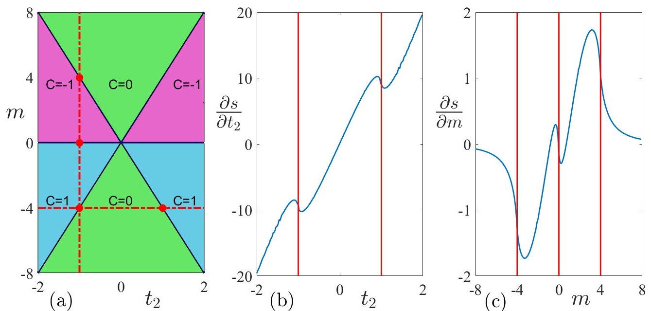
Figure 1: The $m$–$t_{2}$ phase diagram for the spin-orbit Hamiltonian defined by Eq. (1) is shown in (a); different phases are characterized by the Chern numbers $C$. Red dots correspond to critical values of $t_{2}$ and $m$ along the $m=-4t_{1}$ and $t_{2}=-t_{1}$ dashed lines, respectively. The behaviors of $\partial s/\partial t_{2}$ and $\partial s/\partial m$ along these directions are shown in (b) and (c) as a function of $t_{2}$ and $m$, respectively. Red vertical lines represent the phase boundaries, and we set $t=\hbar=t_{1}=1$.

The topology of the Hamiltonian can be characterized by the gauge-dependent Berry connections ${\bm{A}}_{n^{\prime}n}({\bm{k}})\equiv\langle u_{n^{\prime},{\bm{k}}}|i\nabla_{\bm{k}}|u_{n,{\bm{k}}}\rangle$ or the gauge-invariant Berry curvature $\Omega_{n^{\prime}n}({\bm{k}})\equiv\nabla_{\bm{k}}\times{\bm{A}}_{n^{\prime}n}({\bm{k}})$,

$$\Omega({\bm{k}})_{n^{\prime}n} = i\left\langle\frac{\partial u_{n^{\prime},{\bm{k}}}}{\partial k_{x}}\Bigg{|}\frac{\partial u_{n,{\bm{k}}}}{\partial k_{y}}\right\rangle-i\left\langle\frac{\partial u_{n^{\prime},{\bm{k}}}}{\partial k_{y}}\Bigg{|}\frac{\partial u_{n,{\bm{k}}}}{\partial k_{x}}\right\rangle.\hphantom{aaa}$$ (5)

In this work the relevant Chern number is defined as the topological invariant for the lower band $C\equiv(1/2\pi)\int d{\bm{k}}\;\Omega({\bm{k}})_{--}$; note that the sum of lower and upper-band Chern numbers is identically zero. For the model (1), one obtains after some straighforward algebra

$$C=\frac{t_{1}^{2}}{\pi}\int d\bm{k}\frac{2t_{2}\left(\sin k_{x}+\sin k_{y}\right)+m\sin k_{x}\sin k_{y}}{E_{\bm{k}}^{3}}.$$ (6)

This integral that can be readily evaluated numerically, and one obtains $C=\{0,\pm 1\}$ depending on the choice of parameters $t_{2}$ and $m$ in units of $t_{1}$. The resulting phase diagram with regions characterized by different Chern numbers is shown in Fig. 1(a). The boundary between two topologically distinct phases occurs when the gap between the two bands closes, i.e. at the Dirac points $E_{\bm{k}}=0$ for some choice of parameters. Using the definitions (1), the two bands touch at the pair of Dirac points ${\bm{k}}=\left(\pm\frac{\pi}{2},\mp\frac{\pi}{2}\right)$ when $m=0$ and at either of the single Dirac points ${\bm{k}}=\left(\pm\frac{\pi}{2},\pm\frac{\pi}{2}\right)$ for the critical value of $t_{2}$

$$t_{2}^{c\pm}=\mp\frac{m}{4}.$$ (7)

These phase boundaries are shown in Fig. 1(a).

For reasons that will become clear shortly, it is useful to consider the expression for the Chern number close to the phase transition. Choosing fixed $m$ and $t_{2}=t_{2}^{c\pm}+\epsilon$, the leading contribution to the integrand of Eq. (6) comes from ${\bm{k}}$ values where $E_{\bm{k}}$ is minimized; for sufficiently small $\epsilon$, these will be located in the vicinity of the Dirac points. Setting $t_{2}=t_{2}^{c\pm}+\epsilon$, $k_{x}\approx\pm\frac{\pi}{2}+k\cos(\phi)$ and $k_{y}\approx\pm\frac{\pi}{2}+k\sin(\phi)$, one finds that for $|m|/t_{1}\gg 1$ and $k\ll 1$, $E_{\bm{k}}^{2}$ is minimized for $k=k_{c}$, where

$$k_{c}\approx 4\sqrt{\mp\epsilon/m}$$ (8)

or $k_{c}=0$ if the above expression is imaginary. Setting $k=k_{c}$, one obtains $E_{\bm{k}}^{2}\approx 64t_{1}^{2}\left(\mp\epsilon/m\right)$ for $\mp\epsilon/m>0$ and $E_{\bm{k}}^{2}=16\epsilon^{2}$ for $\mp\epsilon/m<0$. To first order in $t_{1}/m$, the integrand of Eq. (6) is highly peaked at $k=k_{c}$ and for $k\sim k_{c}$ is only weakly dependent on angle. Choosing for concreteness $t_{2}=t_{2}^{c+}+\epsilon$, one obtains

$$C\approx\frac{t_{1}^{2}}{2}\int_{0}^{\infty}kdk\frac{16\epsilon-(m+4\epsilon)k^{2}}{\left(a+bk^{2}+ck^{4}\right)^{3/2}},$$ (9)

where $a=16\epsilon^{2}$, $b=4t_{1}^{2}+2m\epsilon-8\epsilon^{2}$, and $c=m^{2}/16-t_{1}^{2}-5m\epsilon/8+3\epsilon^{2}/2$. For $m/t_{1}=-20$, this integral can be readily evaluated numerically, yielding $C\approx 0.012$ and $C\approx 1.002$ for $\epsilon/t_{1}=-0.1$ and $0.1$, respectively. Similar results are obtained for $t_{2}=t_{2}^{c-}+\epsilon$. Thus, near the phase boundary for $|m|/t_{1}\gg 1$, the topological character is extremely well-captured by the lower band structure near the Dirac points.

Of particular interest to the present study is the spatial width of the particle distribution function. While this may be obtained directly from Eq. (4), a detailed calculation (found in the Supplementary Material) shows that at long times the experimentally observable quantity $s$, the time-derivative of the particle variance, depends only on the band structure

$$s\equiv\frac{\hbar^{2}}{t}\frac{\partial}{\partial t}\langle r^{2}\rangle\approx\int\frac{d{\bm{k}}}{(2\pi)^{2}}\left(\nabla_{\bm{k}}E_{\bm{k}}\right)^{2}=\int\frac{d{\bm{k}}}{(4\pi)^{2}}\frac{\left(\nabla_{\bm{k}}E_{\bm{k}}^{2}\right)^{2}}{E_{\bm{k}}^{2}},$$ (10)

and not explicitly on the Berry connections or curvatures. Far from the phase boundary $|t_{2}|\gg\left|t_{2}^{c\pm}\right|$, one can evaluate Eq. (10) analytically in the limit $|m|/t_{1}\gg 1$. One obtains $s=4t_{2}^{2}$ and therefore $\partial s/\partial t_{2}=8t_{2}$, whose linear dependence on $t_{2}$ is confirmed by the numerical results shown in Fig. 1(b). Likewise, it is straightforward to show that $\partial s/\partial m=0$ for $|m|\gg t_{1}$, consistent with the edges of Fig. 1(c).

Pronounced ‘kinks’ in the variations of $\partial s/\partial t_{2}$ with $t_{2}$ and of $\partial s/\partial m$ with $m$ can also be seen in Figs. 1(b) and (c), respectively, clearly revealing the quantum phase transitions. Consider the variation of $\partial s/\partial t_{2}$ with $t_{2}$ (the other case $t_{2}\leftrightarrow m$ proceeds analogously). Close to the phase boundary $t_{2}=t_{2}^{c\pm}+\epsilon$ and considering only $\mp\epsilon/m>0$ (i.e. $C=\pm 1$), one obtains

$$s\approx\frac{512t_{1}^{4}}{\pi}\left(\mp\frac{\epsilon}{m}\right)\int_{0}^{\infty}\frac{kdk}{a+bk^{2}+ck^{4}},$$ (11)

where $a$, $b$, and $c$ take the same values as in Eq. (9). Defining $k^{2}\equiv\sqrt{a/c}x$ the integral is readily evaluated analytically, yielding

$$s\approx\frac{512t_{1}^{4}}{\pi}\left(\mp\frac{\epsilon}{m}\right)\frac{\cos^{-1}\left(b/2\sqrt{ac}\right)}{\sqrt{4ac-b^{2}}}.$$ (12)

Again for $|m|/t_{1}\gg 1$, one has

$$s\approx-\frac{256t_{1}^{4}}{\pi m^{2}}\left(1-\frac{2t_{1}^{2}}{3m\epsilon}\right).$$ (13)

This gives $\partial s/\partial t_{2}\sim\partial s/\partial\epsilon\sim(t_{1}^{6}/|m|^{3})(t_{2}-t_{2}^{c\pm})^{-2}$, which strongly deviates from the linear dependence on $t_{2}$ far from the phase boundary. In fact, the slope of this function is negative, as confirmed by the numerical data presented in Fig. 1(b).

The deviation from the linear $t_{2}$-dependence of $\partial s/\partial t_{2}$ near the phase transition becomes increasingly pronounced as $m$ decreases, which should aid in its experimental detection. Likewise, the signature of the phase transition becomes stronger for higher-order moments $\partial^{k}s/\partial t_{2}^{k}$, though these would likely be difficult to measure precisely in experiments. Though the analytics above only considered the behavior in one phase, the numerical results depicted in Fig. 1(b) and (c) clearly show a similar kink near the boundary for all phases, and one may infer similar behavior for crossings not shown. We have verified similar behavior for the triangular lattice Sticlet2012 which supports states with $C=2$. These findings are consistent with those obtained for one-dimensional systems Cardano2016 . We claim that the numerical and analytical results provide clear evidence that the energy band gap closes; while this is necessary between different topologically ordered phases or between a trivial and non-trivial phase, it is not sufficient to indicate topological order as gap closure could occur between two trivial phases. As such, we will provide additional evidence supporting the topological nature of the phase transition.

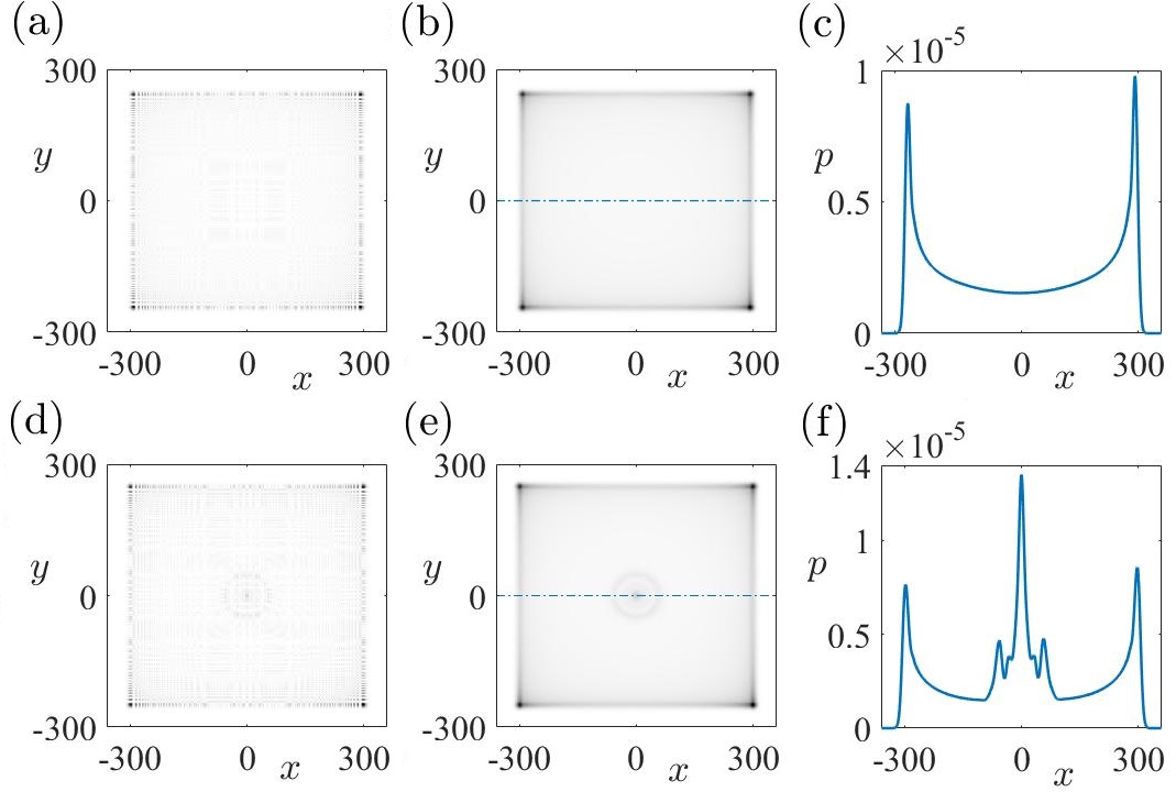
Figure 2: Particle density distributions $p=\langle{\bm{r}}|\psi(t)\rangle|^{2}$. Results for $m=-20t_{1}$ and a $599\times 599$ lattice are shown in (a)-(c) for $t_{2}=4.5t_{1}$ and $t=28\hbar/t_{1}$ ($C=0$), and (d)-(f) for $t_{2}=5.5t_{1}$ and $t=23\hbar/t_{1}$ ($C=1$). Raw data are presented in (a) and (d); smoothed densities in (b) and (e) are obtained by convolving with the function $e^{-(k_{x}^{2}+k_{y}^{2})/\gamma^{2}}$, $\gamma=12.45$, representing the finite resolution of experimental imaging and initial state preparation. Slices through the centers of the particle densities (blue dashed lines) are shown in (c) and (f).

With the appropriate parameter choices, the in situ density profile itself can reveal the nature of the quantum phase, which the average width of the particle distribution cannot. Fig. 2 shows characteristic snapshots of the time-evolved real-space probability $|\langle{\bm{r}}|\psi(t)\rangle|^{2}$ when $|m|/t_{1}\gg 1$, obtained from applying a discrete Fourier transform to $\langle{\bf k}|\psi(t)\rangle$ at long times, subject to ensuring that the leading front of the particle density remains negligible at the edge of the physical lattice. In the trivial phase characterized by $C=0$, Figs. 2(a)-(c), the density is generally featureless with a maximum in the vicinity of the leading edge. This is clearly visible in the slice through the density center, Fig. 2(c) and dovetails with results for a discrete-time quantum walk on a square lattice Watabe2008 . For the free lattice evolution investigated in this work (equivalent to a continuous-time quantum walk) the density profile at long times is square. This result is consistent with experiments on ultracold atoms expanding in a square optical lattice in the absence of particle interactions Schneider2012 , which show little influence on the extent of the initial particle localization. Indeed, choosing a less localized initial state in the numerics, such as a Gaussian distribution with different widths, leads to similar final densities for sufficiently long evolution times (not shown). Likewise, the results hold if the finite resolution of the experimental imaging system and the initial state preparation is taken into account by convolving the particle distribution with a Gaussian $e^{-(k_{x}^{2}+k_{y}^{2})/\gamma^{2}}$, $\gamma=12.45$, representing a generic point-spread function; corresponding results are shown in Fig. 2(b).

In the topologically non-trivial phase with $C=\pm 1$, the time-evolved density profile is similar to that in the trivial phase, but reveals additional rings of high density in the neighborhood of the lattice centre where the particle originated, as shown in Fig. 2(d)-(f). These rings again remain well-defined under changes in initial conditions or under the smoothing due to the finite imaging resolution, Fig. 2(e). While the central peak is clearly visible in the density plots 2(d) and (e), the fainter adjacent ring is more pronounced in the slice through the center, Fig. 2(f). The ring profile is independent of time; the peak positions remain essentially fixed even as the density as a whole expands.

The appearance of these peaks in the density is tied closely to the underlying topology. Because the rotation of the particle spin is tied to its momentum, the time-evolved state $|\psi(t)\rangle$, Eq. (4), becomes a superposition of spin-up and spin-down states. In principle, these can be independently imaged experimentally. Consider first the spin-down component which is initially unpopulated; close to the phase boundary and near the particle origin, the real-space wavefunction is approximately the cylindrical Fourier transform

$$\psi_{\downarrow}(r,t) \approx \frac{it_{1}}{2\pi^{2}}\sin(4\epsilon t/\hbar)\int\frac{kdkd\phi e^{-i\left(\frac{\pi}{2}+k\right)r\cos\phi}ke^{i\phi}}{\sqrt{a+bk^{2}+ck^{4}}}$$ (14)

$$= \frac{t_{1}}{\pi}\sin(4\epsilon t/\hbar)\int_{0}^{\infty}\frac{k^{2}dkJ_{1}\left[r\left(\frac{\pi}{2}+k\right)\right]}{\sqrt{a+bk^{2}+ck^{4}}},$$

with the parameters $a$, $b$, and $c$ again the same as those in Eq. (9) and $J_{1}(x)$ is the Bessel function of the first kind. For $C=\pm 1$, the integrand is dominated by the contribution $k=k_{c}$, Eq. (8). To capture the qualitative properties assume that only the $k=k_{c}$ term contributes; one then obtains

$$\psi_{\downarrow}(r,t)\approx\mp\frac{4t_{1}}{m\pi}\sin\left(\frac{4\epsilon t}{\hbar}\right)J_{1}\left(\frac{\pi r}{2}\right).$$ (15)

The spin-down density for $C=\pm 1$ (for parameters close to the phase boundary) therefore displays a series of concentric rings in the vicinity of the particle origin, spaced by the maxima of the Bessel function. It is straightforward to show that a similar result also holds for the spin-up density, except with the maxima of $J_{0}$ (so that the first maximum is at the origin rather than slightly displaced). In contrast, for $C=0$ all values of $k$ contribute to the integral. The integrand therefore consists of a sum of $J_{\alpha}(kr)$ factors with different values of $k$, which has the effect of smearing out the Bessel function maxima; thus, for $C=0$ the concentric rings are not manifested.

The ring of peaks in the particle distribution appear only in the non-trivial topological phase, but not immediately at the phase boundary. To determine the parameters, it suffices to calculate maxima of the lower band $\nabla_{\bm{k}}E_{\bm{k}}=0$ for $k_{x}=k_{y}$. Simple algebra yields solutions $k_{x}=\left\{\pm\frac{\pi}{2},\sin^{-1}\left[\frac{m(m-4\epsilon)}{(m-4\epsilon)^{2}-8t_{1}^{2}}\right]\right\}$, i.e. the two Dirac points and an additional ring. The last solution is real only if the argument is unity or smaller, which gives $\epsilon\geq-2t_{1}^{2}/m$. Thus, for $|m|/t_{1}\gg 1$, the central peaks manifest themselves almost immediately upon crossing into the non-trivial phase, while for smaller $|m|/t_{1}$ they appear deeper in the phase. These smaller (larger) values of $m$ ($\epsilon$) invalidate the analytical approximations made above, for example neglecting the angular dependence of the energy minima as in Eq. (8), and consequently the central peaks would not be as clearly observable. In practice, the ring features become increasingly washed out for $|m|\lesssim 3t_{1}$ and $|\epsilon|\gtrsim t_{1}$. A similar effect would likely occur for Hamiltonians with closely-spaced Dirac points.

We now argue that the peaks in the particle density obtained above are generic, subject to some restrictions on the choice of Hamiltonian. All of the results hinge on the appearance in the $C\neq 0$ phase of a ring of energy minima at momenta distributed at a radius $k_{c}$ from the Dirac point. Following for instance Sticlet2012 , one can consider ${\bm{h}}({\bm{k}})=(h_{x},h_{y},h_{z})$ as a closed two-dimensional parametric surface ${\mathcal{M}}$, with the Dirac points defined by the origin $(0,0,0)$. The Chern number is then defined as the number of times this oriented surface wraps around the origin; if ${\mathcal{M}}$ touches the origin the band gap closes and $C$ is not defined.

The Hamiltonian (1) belongs to a family of the form $H({\bm{k}})=(h_{x},h_{y},m+t_{2}g_{z})\cdot\bm{\sigma}$, where $h_{x}$, $h_{y}$ and $g_{z}$ are periodic, non-constant functions, symmetric around the $\sigma_{z}$-axis and such that the parametric surface ${\mathcal{M}}$ has a negative-definite curvature. In the large-mass limit $|m|\gg t_{1}$, a topological phase transition is generically characterized by a ring in the energy surface. The phase transition occurs for large $t_{2}^{c}\sim|m|$ from Eq. (7), stretching the surface along the $\sigma_{z}$-axis. The outer points of ${\mathcal{M}}$ are approximately distributed on the surface of a prolate spheroid which passes through the origin as $t_{2}$ increases, changing the Chern number from zero to $\pm 1$. On the trivial side, the energy surface will show a single minimum, corresponding to the outer point of the spheroid. After passing through, a ring of minima appears, symmetric around the $\sigma_{z}$-axis.

The numerical and analytical results presented here indicate that for a realistic (experimentally motivated) spin-orbit lattice Hamiltonian, it is possible to detect transitions between topological phases by allowing particles to evolve freely in the lattice and observe their spatial distribution. The presence of topological order can be inferred from the onset of spatial peaks in the vicinity of the particle origin, which remain well-defined even taking into consideration finite imaging resolution. Similar results are also found for particles hopping on a triangular lattice. This technique is readily applicable to recent ultracold atom experiments Wu2016 and to future implementations using photonic lattices, and should aid in the detection of topological transitions in these systems.

Supplementary Material

Consider a generic (two-dimensional) spin-orbit Hamiltonian. It can be written as

$$H(k_{x},k_{y})=\begin{pmatrix}h_{z}&h_{x}-ih_{y}\cr h_{x}+ih_{y}&-h_{z}\end{pmatrix},$$ (16)

where $h_{i}=h_{i}(k_{x},k_{y})$. This matrix has eigenvalues $E_{\pm}(k_{x},k_{y})=E_{\pm}({\bm{k}})=\pm\sqrt{h_{x}^{2}+h_{y}^{2}+h_{z}^{2}}\equiv\pm E_{\bm{k}}$, and associated eigenvectors

$$|u_{-}\rangle=\sqrt{E_{\bm{k}}+h_{z}\over 2E_{\bm{k}}}\begin{pmatrix}\frac{h_{z}-E_{\bm{k}}}{h_{x}+ih_{y}}\cr 1\end{pmatrix};\qquad|u_{+}\rangle=\sqrt{E_{\bm{k}}-h_{z}\over 2E_{\bm{k}}}\begin{pmatrix}\frac{h_{z}+E_{\bm{k}}}{h_{x}+ih_{y}}\cr 1\end{pmatrix}.$$ (17)

The initial state corresponds to a particle localized to a single lattice point. This lattice point $(0,0)$ has the simplest expression in Fourier coordinates:

$$|0,0\rangle_{x,y}=\sum_{k_{x},k_{y}}|k_{x},k_{y}\rangle,$$ (18)

so that the initial state is an equal superposition of every state in ${\bm{k}}$-space. In addition, suppose the particle starts in spin up:

$$\begin{pmatrix}1\cr 0\end{pmatrix}=\frac{h_{x}+ih_{y}}{\sqrt{2E_{\bm{k}}}}\left(-\frac{1}{\sqrt{E_{\bm{k}}+h_{z}}}|u_{-}\rangle+\frac{1}{\sqrt{E_{\bm{k}}-h_{z}}}|u_{+}\rangle\right).$$ (19)

The (spinor) initial state is therefore

$$|\psi(0)\rangle\equiv\begin{pmatrix}1\cr 0\end{pmatrix}|0,0\rangle_{x,y} = \sum_{k_{x},k_{y}}\frac{h_{x}+ih_{y}}{\sqrt{2E_{\bm{k}}}}\left(-\frac{1}{\sqrt{E_{\bm{k}}+h_{z}}}\langle k_{x},k_{y}|u_{-}\rangle+\frac{1}{\sqrt{E_{\bm{k}}-h_{z}}}\langle k_{x},k_{y}|u_{+}\rangle\right)|k_{x},k_{y}\rangle$$ (20)

$$= \sum_{k_{x},k_{y}}\frac{h_{x}+ih_{y}}{2E_{\bm{k}}}\left[-\begin{pmatrix}\frac{h_{z}-E_{\bm{k}}}{h_{x}+ih_{y}}\cr 1\end{pmatrix}+\begin{pmatrix}\frac{h_{z}+E_{\bm{k}}}{h_{x}+ih_{y}}\cr 1\end{pmatrix}\right]|k_{x},k_{y}\rangle=\sum_{k_{x},k_{y}}\begin{pmatrix}1\cr 0\end{pmatrix}|k_{x},k_{y}\rangle,\hphantom{aa}$$

as expected. Importantly, the initial state is a superposition of both lower ($n=-$) and upper ($n=+$) bands, so the evolution of the position variance with time requires a full mixing of both bands:

$$|\psi(t)\rangle=\sum_{\bm{k}}\frac{h_{x}+ih_{y}}{2E_{\bm{k}}}\left[-e^{iE_{\bm{k}}t/\hbar}\begin{pmatrix}\frac{h_{z}-E_{\bm{k}}}{h_{x}+ih_{y}}\cr 1\end{pmatrix}+e^{-iE_{\bm{k}}t/\hbar}\begin{pmatrix}\frac{h_{z}+E_{\bm{k}}}{h_{x}+ih_{y}}\cr 1\end{pmatrix}\right]|{\bm{k}}\rangle.$$ (21)

Also, the expressions for the $u_{\pm}(k_{x},k_{y})\equiv\langle k_{x},k_{y}|u_{\pm}\rangle$ are non-separable, i.e. one cannot write $u_{-}(k_{x},k_{y})=u_{-}(k_{x})u_{-}(k_{y})$ and similarly for $u_{+}(k_{x},k_{y})$.

The expressions for the Bloch functions (17) allow us to calculate the Berry connections. After some algebraic manipulations one obtains

$$A_{x}({\bm{k}})_{--} \equiv \left\langle u_{-}\bigg{|}i\frac{\partial}{\partial k_{x}}\bigg{|}u_{-}\right\rangle=\frac{1}{2E_{\bm{k}}(E_{\bm{k}}+h_{z})}\left(h_{x}\frac{\partial h_{y}}{\partial k_{x}}-h_{y}\frac{\partial h_{x}}{\partial k_{x}}\right);$$

$$A_{x}({\bm{k}})_{++} \equiv \left\langle u_{+}\bigg{|}i\frac{\partial}{\partial k_{x}}\bigg{|}u_{+}\right\rangle=\frac{1}{2E_{\bm{k}}(E_{\bm{k}}-h_{z})}\left(h_{x}\frac{\partial h_{y}}{\partial k_{x}}-h_{y}\frac{\partial h_{x}}{\partial k_{x}}\right).$$ (22)

The expressions for $A_{y}$ are obtained analogously, by replacing the $k_{x}$-derivatives by $k_{y}$-derivatives. Note that these intra-band Berry connections are purely real, as expected from the fact that $\langle u_{n}|i\partial/\partial k_{i}|u_{n}\rangle^{{\dagger}}=\langle u_{n}|i\partial/\partial k_{i}|u_{n}\rangle$ (the real $x$ operator maps to $i\partial/\partial k_{x}$). The corresponding inter-band Berry connections are

$$A_{x}({\bm{k}})_{+-} \equiv \left\langle u_{+}\bigg{|}i\frac{\partial}{\partial k_{x}}\bigg{|}u_{-}\right\rangle=-\frac{1}{2E_{\bm{k}}\sqrt{h_{x}^{2}+h_{y}^{2}}}\left[h_{x}\frac{\partial h_{y}}{\partial k_{x}}-h_{y}\frac{\partial h_{x}}{\partial k_{x}}+i\left(h_{z}\frac{\partial E_{\bm{k}}}{\partial k_{x}}-E_{\bm{k}}\frac{\partial h_{z}}{\partial k_{x}}\right)\right];$$

$$A_{x}({\bm{k}})_{-+} \equiv \left\langle u_{-}\bigg{|}i\frac{\partial}{\partial k_{x}}\bigg{|}u_{+}\right\rangle=-\frac{1}{2E_{\bm{k}}\sqrt{h_{x}^{2}+h_{y}^{2}}}\left[h_{x}\frac{\partial h_{y}}{\partial k_{x}}-h_{y}\frac{\partial h_{x}}{\partial k_{x}}-i\left(h_{z}\frac{\partial E_{\bm{k}}}{\partial k_{x}}-E_{\bm{k}}\frac{\partial h_{z}}{\partial k_{x}}\right)\right].$$ (23)

Again, the expressions for $A_{y}({\bm{k}})_{nn^{\prime}}$ are obtained by replacing $k_{x}$-derivatives with $k_{y}$-derivatives. The inter-band Berry connections properly satisfy the expected relationship $A_{i}({\bm{k}})_{nn^{\prime}}^{*}=A_{i}({\bm{k}})_{n^{\prime}n}$, $n\neq n^{\prime}$. Surprisingly, however, they are complex quantities. That said, the real parts are proportional to their intra-band counterparts. The Berry curvature is defined as

$$\Omega({\bm{k}})_{n^{\prime}n}=\left[\nabla_{k}\times{\bm{A}}({\bm{k}})\right]_{n^{\prime}n}=\frac{\partial}{\partial k_{x}}A_{y}({\bm{k}})_{n^{\prime}n}-\frac{\partial}{\partial k_{y}}A_{x}({\bm{k}})_{n^{\prime}n}.$$ (24)

After some algebra, the Berry curvature of interest takes the simple and intuitive form:

$$\Omega({\bm{k}})_{--}=\frac{1}{2E_{\bm{k}}^{3}}\left[h_{x}\left(\frac{\partial h_{y}}{\partial k_{x}}\frac{\partial h_{z}}{\partial k_{y}}-\frac{\partial h_{y}}{\partial k_{y}}\frac{\partial h_{z}}{\partial k_{x}}\right)+h_{y}\left(\frac{\partial h_{z}}{\partial k_{x}}\frac{\partial h_{x}}{\partial k_{y}}-\frac{\partial h_{z}}{\partial k_{y}}\frac{\partial h_{x}}{\partial k_{x}}\right)+h_{z}\left(\frac{\partial h_{x}}{\partial k_{x}}\frac{\partial h_{y}}{\partial k_{y}}-\frac{\partial h_{x}}{\partial k_{y}}\frac{\partial h_{y}}{\partial k_{x}}\right)\right].$$ (25)

Let’s consider the second term of Eq. (24):

$$-\frac{\partial}{\partial k_{y}}A_{x}({\bm{k}})_{n^{\prime}n} = -\sum_{\sigma}\left[\left(\frac{\partial}{\partial k_{y}}u^{*}_{n^{\prime},{\bm{k}},\sigma}\right)i\frac{\partial}{\partial k_{x}}u_{n,{\bm{k}},\sigma}+u^{*}_{n^{\prime},{\bm{k}},\sigma}i\frac{\partial^{2}}{\partial k_{x}k_{y}}u_{n,{\bm{k}},\sigma}\right)$$ (26)

$$= -i\left\langle\frac{\partial}{\partial k_{y}}u_{n^{\prime},{\bm{k}}}\Bigg{|}\frac{\partial}{\partial k_{x}}u_{n,{\bm{k}}}\right\rangle-i\left\langle u_{n^{\prime},{\bm{k}}}\Bigg{|}\frac{\partial^{2}}{\partial k_{y}k_{x}}u_{n,{\bm{k}}}\right\rangle.$$

The first term follows by interchanging $k_{x}\leftrightarrow k_{y}$:

$$\frac{\partial}{\partial k_{x}}A_{y}({\bm{k}})_{n^{\prime}n} = \sum_{\sigma}\left[\left(\frac{\partial}{\partial k_{x}}u^{*}_{n^{\prime},{\bm{k}},\sigma}\right)i\frac{\partial}{\partial k_{y}}u_{n,{\bm{k}},\sigma}+u^{*}_{n^{\prime},{\bm{k}},\sigma}i\frac{\partial^{2}}{\partial k_{x}k_{y}}u_{n,{\bm{k}},\sigma}\right)$$ (27)

$$= i\left\langle\frac{\partial}{\partial k_{x}}u_{n^{\prime},{\bm{k}}}\Bigg{|}\frac{\partial}{\partial k_{y}}u_{n,{\bm{k}}}\right\rangle+i\left\langle u_{n^{\prime},{\bm{k}}}\Bigg{|}\frac{\partial^{2}}{\partial k_{x}k_{y}}u_{n,{\bm{k}}}\right\rangle.$$

Because $\frac{\partial^{2}}{\partial k_{x}k_{y}}=\frac{\partial^{2}}{\partial k_{y}k_{x}}$ one obtains

$$\Omega({\bm{k}})_{z,n^{\prime}n}=i\left\langle\frac{\partial}{\partial k_{x}}u_{n^{\prime},{\bm{k}}}\Bigg{|}\frac{\partial}{\partial k_{y}}u_{n,{\bm{k}}}\right\rangle-i\left\langle\frac{\partial}{\partial k_{y}}u_{n^{\prime},{\bm{k}}}\Bigg{|}\frac{\partial}{\partial k_{x}}u_{n,{\bm{k}}}\right\rangle,$$ (28)

which is the well-known expression.

We would like to calculate the time-dependent expectation value of

$$\langle r^{2}\rangle=\langle x^{2}+y^{2}\rangle=\langle\psi(t)|x^{2}+y^{2}|\psi(t)\rangle=\sum_{{\bm{r}},{\bm{r}}^{\prime}}\langle\psi(t)|{\bm{r}}\rangle\langle{\bm{r}}|x^{2}+y^{2}|{\bm{r}}^{\prime}\rangle\langle{\bm{r}}^{\prime}|\psi(t)\rangle=\sum_{{\bm{r}},\sigma}\psi_{\sigma}^{*}({\bm{r}},t)(x^{2}+y^{2})\psi_{\sigma}({\bm{r}},t),$$ (29)

to find out the dependence on the Berry curvature (if any). Here the sum over $\sigma$ corresponds to adding the two components $-$ and $+$ of the two-band state. The state $\psi_{\sigma}({\bm{r}},t)$ can be expressed as

$$\psi_{\sigma}({\bm{r}},t)=\sum_{n}\sum_{{\bm{k}}}a_{n}({\bm{k}},t)\psi_{n,{\bm{k}},\sigma}({\bm{r}}),$$ (30)

where the arbitrary state is expanded in a complete basis set,

$$\sum_{{\bm{r}},\sigma}\psi^{*}_{n^{\prime},{\bm{k}}^{\prime},\sigma}({\bm{r}})\psi_{n,{\bm{k}},\sigma}({\bm{r}})=\delta_{n,n^{\prime}}\delta({\bm{k}}^{\prime}-{\bm{k}}).$$ (31)

Note that the states $\psi_{n,{\bm{k}},\sigma}({\bm{r}})$ are the components of the solutions of the full Hamiltonian on the lattice,

$$H|\psi_{n,{\bm{k}}}\rangle=E_{n}({\bm{k}})|\psi_{n,{\bm{k}}}\rangle,$$ (32)

where $\psi_{n,{\bm{k}},\sigma}({\bm{r}})=\langle{\bm{r}},\sigma|\psi_{n,{\bm{k}}}\rangle$. These basis function are not translationally invariant because according to Bloch’s theorem

$$\psi_{n,{\bm{k}},\sigma}({\bm{r}}+{\bm{R}})=e^{i{\bm{k}}\cdot{\bm{R}}}\psi_{n,{\bm{k}},\sigma}({\bm{r}}),$$ (33)

where ${\bm{R}}$ is an arbitrary unit cell lattice vector. So it is more convenient to expand in translationally invariant Bloch functions where $\psi_{n,{\bm{k}},\sigma}({\bm{r}})\equiv e^{i{\bm{k}}\cdot{\bm{r}}}u_{n,{\bm{k}},\sigma}({\bm{r}})$, where the functions satisfy $u_{n,{\bm{k}},\sigma}({\bm{r}}+{\bm{R}})=u_{n,{\bm{k}},\sigma}({\bm{r}})$. It’s clear that this definition is consistent with Eq. (33). Also because these functions have the same value for any ${\bm{r}}$ we can drop the ${\bm{r}}$-dependence completely. Note that these basis functions are the eigenfunctions of the ${\bm{k}}$-dependent Hamiltonian $H({\bm{k}})\equiv e^{-i{\bm{k}}\cdot{\bm{r}}}He^{i{\bm{k}}\cdot{\bm{r}}}$:

$$H({\bm{k}})|u_{n,{\bm{k}}}\rangle=E_{n}({\bm{k}})|u_{n,{\bm{k}}}\rangle.$$ (34)

The definition of the arbitrary function, Eq. (30), then becomes

$$\psi_{\sigma}({\bm{r}},t)=\sum_{n}\sum_{\bm{k}}a_{n}({\bm{k}},t)e^{i{\bm{k}}\cdot{\bm{r}}}u_{n,{\bm{k}},\sigma}.$$ (35)

Comparison of Eqs. (19) and (35) (recall that $|{\bm{r}}|=0$) gives

$$a_{-}(k_{x},k_{y})=-\frac{h_{x}+ih_{y}}{\sqrt{2E_{\bm{k}}(E_{\bm{k}}+h_{z})}};\quad a_{+}(k_{x},k_{y})=\frac{h_{x}+ih_{y}}{\sqrt{2E_{\bm{k}}(E_{\bm{k}}-h_{z})}}.$$ (36)

for the particular problem of interest. The orthogonality condition (31) then becomes

$$\sum_{{\bm{r}},\sigma}e^{i({\bm{k}}-{\bm{k}}^{\prime})\cdot{\bm{r}}}u^{*}_{n^{\prime},{\bm{k}}^{\prime},\sigma}({\bm{r}})u_{n,{\bm{k}},\sigma}({\bm{r}})=\delta_{n,n^{\prime}}\delta({\bm{k}}^{\prime}-{\bm{k}}).$$ (37)

But on a lattice the $u_{n,{\bm{k}},\sigma}({\bm{r}})$ have the same value for any ${\bm{r}}$; the ${\bm{r}}$-dependence can therefore be dropped, and one obtains

$$\sum_{{\bm{r}},\sigma}e^{i({\bm{k}}-{\bm{k}}^{\prime})\cdot{\bm{r}}}u^{*}_{n^{\prime},{\bm{k}}^{\prime},\sigma}u_{n,{\bm{k}},\sigma}=\langle u_{n^{\prime},{\bm{k}}^{\prime}}|u_{n,{\bm{k}}}\rangle\sum_{{\bm{r}}}e^{i({\bm{k}}-{\bm{k}}^{\prime})\cdot{\bm{r}}}=\langle u_{n^{\prime},{\bm{k}}^{\prime}}|u_{n,{\bm{k}}}\rangle\delta({\bm{k}}-{\bm{k}}^{\prime})=\delta_{n,n^{\prime}}\delta({\bm{k}}^{\prime}-{\bm{k}}).$$ (38)

Eq. (29) is then written

$$\left\langle x^{2}+y^{2}\right\rangle = \sum_{{\bm{r}},\sigma}\sum_{n,n^{\prime}}\sum_{\bm{k}}\sum_{{\bm{k}}^{\prime}}a^{*}_{n^{\prime}}({\bm{k}}^{\prime},t)\psi^{*}_{n^{\prime},{\bm{k}}^{\prime},\sigma}({\bm{r}})(x^{2}+y^{2})a_{n}({\bm{k}},t)\psi_{n,{\bm{k}},\sigma}({\bm{r}})$$ (39)

$$= \sum_{{\bm{r}},\sigma}\sum_{n,n^{\prime}}\sum_{\bm{k}}\sum_{{\bm{k}}^{\prime}}a^{*}_{n^{\prime}}({\bm{k}}^{\prime},t)a_{n}({\bm{k}},t)e^{-i{\bm{k}}^{\prime}\cdot{\bm{r}}}u^{*}_{n^{\prime},{\bm{k}}^{\prime},\sigma}(x^{2}+y^{2})e^{i{\bm{k}}\cdot{\bm{r}}}u_{n,{\bm{k}},\sigma}.$$

It is convenient to focus on one dimension at a time.

$$\left\langle x^{2}\right\rangle = \sum_{x,\sigma}\sum_{n,n^{\prime}}\sum_{\bm{k}}\sum_{{\bm{k}}^{\prime}}a^{*}_{n^{\prime}}({\bm{k}}^{\prime},t)a_{n}({\bm{k}},t)e^{-ik_{x}^{\prime}x}u^{*}_{n^{\prime},{\bm{k}}^{\prime},\sigma}x^{2}e^{ik_{x}x}u_{n,{\bm{k}},\sigma}\sum_{y}e^{i(k_{y}-k_{y}^{\prime})y}$$ (40)

$$= \sum_{x,\sigma}\sum_{n,n^{\prime}}\sum_{\bm{k}}\sum_{{\bm{k}}^{\prime}}a^{*}_{n^{\prime}}({\bm{k}}^{\prime},t)a_{n}({\bm{k}},t)e^{-ik_{x}^{\prime}x}u^{*}_{n^{\prime},{\bm{k}}^{\prime},\sigma}x^{2}e^{ik_{x}x}u_{n,{\bm{k}},\sigma}\delta(k_{y}-k_{y}^{\prime})$$

$$= \sum_{n,n^{\prime}}\sum_{k_{x},k_{x}^{\prime}}\sum_{k_{y}}a^{*}_{n^{\prime}}(k_{x}^{\prime},k_{y},t)a_{n}(k_{x},k_{y},t)\sum_{x,\sigma}e^{-ik_{x}^{\prime}x}u^{*}_{n^{\prime},k_{x}^{\prime},k_{y},\sigma}x^{2}e^{ik_{x}x}u_{n,k_{x},k_{y},\sigma}.$$

Note that we could equivalently express the final sum as

$$\sum_{x,\sigma}\psi^{*}_{n^{\prime},k_{x}^{\prime},k_{y},\sigma}(x)x^{2}\psi_{n,k_{x},k_{y},\sigma}(x)=\sum_{x,x^{\prime}}\langle\psi_{n^{\prime},k_{x}^{\prime},k_{y}}|x\rangle\langle x|x^{2}|x^{\prime}\rangle\langle x^{\prime}|\psi_{n,k_{x},k_{y}}\rangle=\langle\psi_{n^{\prime},k_{x}^{\prime},k_{y}}|x^{2}|\psi_{n,k_{x},k_{y}}\rangle.$$ (41)

To proceed, note that:

$$\frac{\partial^{2}}{\partial k_{x}^{2}}\sum_{x,\sigma}\psi^{*}_{n^{\prime},k_{x}^{\prime},k_{y},\sigma}(x)\psi_{n,k_{x},k_{y},\sigma}(x) = \frac{\partial^{2}}{\partial k_{x}^{2}}\sum_{x,\sigma}e^{-ik_{x}^{\prime}x}u^{*}_{n^{\prime},k_{x}^{\prime},k_{y},\sigma}e^{ik_{x}x}u_{n,k_{x},k_{y}}$$

$$= \sum_{x,\sigma}e^{-ik_{x}^{\prime}x}u^{*}_{n^{\prime},k_{x}^{\prime},k_{y},\sigma}\frac{\partial^{2}}{\partial k_{x}^{2}}\left[e^{ik_{x}x}u_{n,k_{x},k_{y},\sigma}\right]$$

$$= \sum_{x,\sigma}e^{-ik_{x}^{\prime}x}u^{*}_{n^{\prime},k_{x}^{\prime},k_{y},\sigma}\frac{\partial}{\partial k_{x}}\left[ixe^{ik_{x}x}u_{n,k_{x},k_{y},\sigma}+e^{ik_{x}x}\frac{\partial}{\partial k_{x}}u_{n,k_{x},k_{y},\sigma}\right]$$

$$= \sum_{x,\sigma}e^{-ik_{x}^{\prime}x}u^{*}_{n^{\prime},k_{x}^{\prime},k_{y},\sigma}\left[-x^{2}e^{ik_{x}x}+2ixe^{ik_{x}x}\frac{\partial}{\partial k_{x}}+e^{ik_{x}x}\frac{\partial^{2}}{\partial k_{x}^{2}}\right]u_{n,k_{x},k_{y},\sigma},$$

so that

$$\sum_{x,\sigma}\psi^{*}_{n^{\prime},k_{x}^{\prime},k_{y},\sigma}(x)x^{2}\psi_{n,k_{x},k_{y},\sigma}(x) = \sum_{x,\sigma}e^{i(k_{x}-k_{x}^{\prime})x}u^{*}_{n^{\prime},k_{x}^{\prime},k_{y},\sigma}\left[2ix\frac{\partial}{\partial k_{x}}+\frac{\partial^{2}}{\partial k_{x}^{2}}\right]u_{n,k_{x},k_{y},\sigma}$$ (42)

$$- \frac{\partial^{2}}{\partial k_{x}^{2}}\sum_{x,\sigma}\psi^{*}_{n^{\prime},k_{x}^{\prime},k_{y},\sigma}(x)\psi_{n,k_{x},k_{y},\sigma}(x).$$

The first two terms are not manifestly Hermitian, however. If one had taken derivatives with respect to $k_{x}^{\prime}$ instead, one would have instead obtained

$$\sum_{x,\sigma}\psi^{*}_{n^{\prime},k_{x}^{\prime},k_{y},\sigma}(x)x^{2}\psi_{n,k_{x},k_{y},\sigma}(x) = \sum_{x,\sigma}e^{i(k_{x}-k_{x}^{\prime})x}u_{n,k_{x},k_{y},\sigma}\left[-2ix\frac{\partial}{\partial k_{x}^{\prime}}+\frac{\partial^{2}}{\partial{k_{x}^{\prime}}^{2}}\right]u^{*}_{n^{\prime},k_{x}^{\prime},k_{y},\sigma}$$ (43)

$$- \frac{\partial^{2}}{\partial{k_{x}^{\prime}}^{2}}\sum_{x,\sigma}\psi^{*}_{n^{\prime},k_{x}^{\prime},k_{y},\sigma}(x)\psi_{n,k_{x},k_{y},\sigma}(x).$$

The last sum gives $\delta(k_{x}-k_{x}^{\prime})\delta_{n,n^{\prime}}$ from Eq. (31). For the second term, because the sum over $x$ is over all space, we can set $x=x^{\prime}+R_{x}$, where $R_{x}$ is a translation by an arbitrary number of unit cell lengths and $x^{\prime}$ is restricted to a single unit cell. Then

$$\sum_{x,\sigma}e^{i(k_{x}-k_{x}^{\prime})x}u^{*}_{n^{\prime},k_{x}^{\prime},k_{y},\sigma}\frac{\partial^{2}}{\partial k_{x}^{2}}u_{n,k_{x},k_{y},\sigma} = \sum_{R_{x}}e^{i(k_{x}-k_{x}^{\prime})R_{x}}\sum_{x^{\prime},\sigma}e^{i(k_{x}-k_{x}^{\prime})x^{\prime}}u^{*}_{n^{\prime},k_{x}^{\prime},k_{y},\sigma}\frac{\partial^{2}}{\partial k_{x}^{2}}u_{n,k_{x},k_{y},\sigma}$$ (44)

$$= \delta(k_{x}-k_{x}^{\prime})\sum_{x\in{\rm u.c.},\sigma}e^{i(k_{x}-k_{x}^{\prime})x}u^{*}_{n^{\prime},k_{x}^{\prime},k_{y},\sigma}\frac{\partial^{2}}{\partial k_{x}^{2}}u_{n,k_{x},k_{y},\sigma}$$

$$= \delta(k_{x}-k_{x}^{\prime})\sum_{x\in{\rm u.c.},\sigma}u^{*}_{n^{\prime},k_{x}^{\prime},k_{y},\sigma}\frac{\partial^{2}}{\partial k_{x}^{2}}u_{n,k_{x},k_{y},\sigma},$$

where the sum is now only over a single unit cell rather than over all space. In the last line we have made use of the fact that $k_{x}=k_{x}^{\prime}$. Inserting these results into the previous expression gives

$$\sum_{x,\sigma}\psi^{*}_{n^{\prime},k_{x}^{\prime},k_{y},\sigma}(x)x^{2}\psi_{n,k_{x},k_{y},\sigma}(x) = \delta(k_{x}-k_{x}^{\prime})\frac{1}{2}\sum_{x\in{\rm u.c.,\sigma}}\left(u^{*}_{n^{\prime},k_{x}^{\prime},k_{y},\sigma}\frac{\partial^{2}}{\partial k_{x}^{2}}u_{n,k_{x},k_{y},\sigma}+u_{n,k_{x},k_{y},\sigma}\frac{\partial^{2}}{\partial{k_{x}^{\prime}}^{2}}u^{*}_{n^{\prime},k_{x}^{\prime},k_{y},\sigma}\right)$$ (45)

$$- \delta_{n,n^{\prime}}\frac{1}{2}\left(\frac{\partial^{2}}{\partial k_{x}^{2}}+\frac{\partial^{2}}{\partial{k_{x}^{\prime}}^{2}}\right)\delta(k_{x}-k_{x}^{\prime})$$

$$+ \sum_{x,\sigma}e^{i(k_{x}-k_{x}^{\prime})x}ix\left(u^{*}_{n^{\prime},k_{x}^{\prime},k_{y},\sigma}\frac{\partial}{\partial k_{x}}u_{n,k_{x},k_{y},\sigma}-u_{n,k_{x},k_{y},\sigma}\frac{\partial}{\partial k_{x}^{\prime}}u^{*}_{n^{\prime},k_{x}^{\prime},k_{y},\sigma}\right)$$

$$= \delta(k_{x}-k_{x}^{\prime})\frac{1}{2}\sum_{x\in{\rm u.c.,\sigma}}\left(u^{*}_{n^{\prime},k_{x}^{\prime},k_{y},\sigma}\frac{\partial^{2}}{\partial k_{x}^{2}}u_{n,k_{x},k_{y},\sigma}+u_{n,k_{x},k_{y},\sigma}\frac{\partial^{2}}{\partial{k_{x}^{\prime}}^{2}}u^{*}_{n^{\prime},k_{x}^{\prime},k_{y},\sigma}\right)$$

$$- \delta_{n,n^{\prime}}\frac{1}{2}\left(\frac{\partial^{2}}{\partial k_{x}^{2}}+\frac{\partial^{2}}{\partial{k_{x}^{\prime}}^{2}}\right)\delta(k_{x}-k_{x}^{\prime})$$

$$+ \sum_{x,\sigma}e^{-ik_{x}^{\prime}x}u^{*}_{n^{\prime},k_{x}^{\prime},k_{y},\sigma}\left(\frac{\partial}{\partial k_{x}}e^{ik_{x}x}\right)\frac{\partial}{\partial k_{x}}u_{n,k_{x},k_{y},\sigma}$$

$$+ \sum_{x,\sigma}\left(\frac{\partial}{\partial k_{x}^{\prime}}e^{-ik_{x}^{\prime}x}\right)e^{ik_{x}x}u_{n,k_{x},k_{y},\sigma}\frac{\partial}{\partial k_{x}^{\prime}}u^{*}_{n^{\prime},k_{x}^{\prime},k_{y},\sigma},$$

which is manifestly Hermitian. Inserting this into the full expression for $\langle x^{2}\rangle$ gives

$$\left\langle x^{2}\right\rangle = \sum_{n,n^{\prime}}\sum_{k_{x},k_{x}^{\prime}}\sum_{k_{y}}a^{*}_{n^{\prime}}(k_{x}^{\prime},k_{y},t)a_{n}(k_{x},k_{y},t)\delta(k_{x}-k_{x}^{\prime})\sum_{\sigma}\frac{1}{2}\left(u^{*}_{n^{\prime},k_{x}^{\prime},k_{y},\sigma}\frac{\partial^{2}}{\partial k_{x}^{2}}u_{n,k_{x},k_{y},\sigma}+u_{n,k_{x},k_{y},\sigma}\frac{\partial^{2}}{\partial k_{x}^{2}}u^{*}_{n^{\prime},k_{x}^{\prime},k_{y},\sigma}\right)$$ (46)

$$- \frac{1}{2}\sum_{n,n^{\prime}}\sum_{k_{x},k_{x}^{\prime}}\sum_{k_{y}}a^{*}_{n^{\prime}}(k_{x}^{\prime},k_{y},t)a_{n}(k_{x},k_{y},t)\left(\frac{\partial^{2}}{\partial k_{x}^{2}}+\frac{\partial^{2}}{\partial{k_{x}^{\prime}}^{2}}\right)\delta(k_{x}-k_{x}^{\prime})\delta_{n,n^{\prime}}$$

$$+ \sum_{n,n^{\prime}}\sum_{k_{x},k_{x}^{\prime}}\sum_{k_{y}}a^{*}_{n^{\prime}}(k_{x}^{\prime},k_{y},t)a_{n}(k_{x},k_{y},t)\sum_{x,\sigma}e^{-ik_{x}^{\prime}x}u^{*}_{n^{\prime},k_{x}^{\prime},k_{y},\sigma}\left(\frac{\partial}{\partial k_{x}}e^{ik_{x}x}\right)\frac{\partial}{\partial k_{x}}u_{n,k_{x},k_{y},\sigma}$$

$$+ \sum_{n,n^{\prime}}\sum_{k_{x},k_{x}^{\prime}}\sum_{k_{y}}a^{*}_{n^{\prime}}(k_{x}^{\prime},k_{y},t)a_{n}(k_{x},k_{y},t)\sum_{x,\sigma}\left(\frac{\partial}{\partial k_{x}^{\prime}}e^{-ik_{x}^{\prime}x}\right)u_{n,k_{x},k_{y},\sigma}\frac{\partial}{\partial k_{x}^{\prime}}u^{*}_{n^{\prime},k_{x}^{\prime},k_{y},\sigma}e^{ik_{x}x}.$$

To evaluate the second line, we can use the identity

$$\sum_{x}f(x)\delta^{(n)}(x-x_{0})=(-1)^{n}f^{(n)}(x_{0}),$$ (47)

which can be verified by integrating by parts $n$ times. Likewise, one can integrate the last two terms by parts once. One then obtains

$$\left\langle x^{2}\right\rangle = \frac{1}{2}\sum_{n,n^{\prime}}\sum_{\bm{k}}\left(a^{*}_{n^{\prime}}({\bm{k}},t)a_{n}({\bm{k}},t)\sum_{\sigma}u^{*}_{n^{\prime},{\bm{k}},\sigma}\frac{\partial^{2}}{\partial k_{x}^{2}}u_{n,{\bm{k}},\sigma}+{\rm H.c.}^{\prime}\right)-\frac{1}{2}\sum_{n}\sum_{\bm{k}}\left(a^{*}_{n}({\bm{k}},t)\frac{\partial^{2}}{\partial k_{x}^{2}}a_{n}({\bm{k}},t)+{\rm H.c.}^{\prime}\right)$$ (48)

$$- \sum_{n,n^{\prime}}\sum_{k_{x},k_{x}^{\prime}}\sum_{k_{y}}a^{*}_{n^{\prime}}(k_{x}^{\prime},k_{y},t)\sum_{x,\sigma}e^{i(k_{x}-k_{x}^{\prime})x}u^{*}_{n^{\prime},k_{x}^{\prime},k_{y},\sigma}\frac{\partial}{\partial k_{x}}\left(a_{n}(k_{x},k_{y},t)\frac{\partial}{\partial k_{x}}u_{n,k_{x},k_{y},\sigma}\right)$$

$$- \sum_{n,n^{\prime}}\sum_{k_{x},k_{x}^{\prime}}\sum_{k_{y}}a_{n}(k_{x},k_{y},t)\sum_{x,\sigma}e^{i(k_{x}-k_{x}^{\prime})x}u_{n,k_{x},k_{y},\sigma}\frac{\partial}{\partial k_{x}^{\prime}}\left(a^{*}_{n^{\prime}}(k_{x}^{\prime},k_{y},t)\frac{\partial}{\partial k_{x}^{\prime}}u^{*}_{n^{\prime},k_{x}^{\prime},k_{y},\sigma}\right)$$

$$= \frac{1}{2}\sum_{n,n^{\prime}}\sum_{\bm{k}}\left(a^{*}_{n^{\prime}}({\bm{k}},t)a_{n}({\bm{k}},t)\sum_{\sigma}u^{*}_{n^{\prime},{\bm{k}},\sigma}\frac{\partial^{2}}{\partial k_{x}^{2}}u_{n,{\bm{k}},\sigma}+{\rm H.c.}^{\prime}\right)-\frac{1}{2}\sum_{n}\sum_{\bm{k}}\left(a^{*}_{n}({\bm{k}},t)\frac{\partial^{2}}{\partial k_{x}^{2}}a_{n}({\bm{k}},t)+{\rm H.c.}^{\prime}\right)$$

$$- \sum_{n,n^{\prime}}\sum_{{\bm{k}}}a^{*}_{n^{\prime}}({\bm{k}},t)\sum_{\sigma}u^{*}_{n^{\prime},{\bm{k}},\sigma}\left(\frac{\partial}{\partial k_{x}}a_{n}({\bm{k}},t)\frac{\partial}{\partial k_{x}}u_{n,{\bm{k}},\sigma}+a_{n}({\bm{k}},t)\frac{\partial^{2}}{\partial k_{x}^{2}}u_{n,{\bm{k}},\sigma}\right)$$

$$- \sum_{n,n^{\prime}}\sum_{{\bm{k}}}a_{n}({\bm{k}},t)\sum_{\sigma}u_{n,{\bm{k}},\sigma}\left(\frac{\partial}{\partial k_{x}}a^{*}_{n^{\prime}}({\bm{k}},t)\frac{\partial}{\partial k_{x}}u^{*}_{n^{\prime},{\bm{k}},\sigma}+a^{*}_{n^{\prime}}({\bm{k}},t)\frac{\partial^{2}}{\partial k_{x}^{2}}u^{*}_{n^{\prime},{\bm{k}},\sigma}\right)$$

$$= -\frac{1}{2}\sum_{n,n^{\prime}}\sum_{\bm{k}}\left(a^{*}_{n^{\prime}}({\bm{k}},t)a_{n}({\bm{k}},t)\sum_{\sigma}u^{*}_{n^{\prime},{\bm{k}},\sigma}\frac{\partial^{2}}{\partial k_{x}^{2}}u_{n,{\bm{k}},\sigma}+{\rm H.c.}^{\prime}\right)-\frac{1}{2}\sum_{n}\sum_{\bm{k}}\left(a^{*}_{n}({\bm{k}},t)\frac{\partial^{2}}{\partial k_{x}^{2}}a_{n}({\bm{k}},t)+{\rm H.c.}^{\prime}\right)$$

$$- \sum_{n,n^{\prime}}\sum_{{\bm{k}}}\left(a^{*}_{n^{\prime}}({\bm{k}},t)\frac{\partial}{\partial k_{x}}a_{n}({\bm{k}},t)\sum_{\sigma}u^{*}_{n^{\prime},{\bm{k}},\sigma}\frac{\partial}{\partial k_{x}}u_{n,{\bm{k}},\sigma}+{\rm H.c.}^{\prime}\right),$$

where the notation ${\rm H.c.}^{\prime}$ represents complex conjugation of all quantities as well as the interchange of band labels $n\leftrightarrow n^{\prime}$ (these are dummy indices). The expectation of $r^{2}$ is therefore

$$\langle r^{2}\rangle = -\frac{1}{2}\sum_{n,n^{\prime}}\sum_{\bm{k}}\left(a^{*}_{n^{\prime}}({\bm{k}},t)a_{n}({\bm{k}},t)\sum_{\sigma}u^{*}_{n^{\prime},{\bm{k}},\sigma}\nabla_{\bm{k}}^{2}u_{n,{\bm{k}},\sigma}+{\rm H.c.}^{\prime}\right)-\frac{1}{2}\sum_{n}\sum_{\bm{k}}\left(a^{*}_{n}({\bm{k}},t)\nabla_{\bm{k}}^{2}a_{n}({\bm{k}},t)+{\rm H.c.}^{\prime}\right)$$ (49)

$$- \sum_{n,n^{\prime}}\sum_{{\bm{k}}}\left(a^{*}_{n^{\prime}}({\bm{k}},t)\nabla_{\bm{k}}a_{n}({\bm{k}},t)\cdot\sum_{\sigma}u^{*}_{n^{\prime},{\bm{k}},\sigma}\nabla_{\bm{k}}u_{n,{\bm{k}},\sigma}+{\rm H.c.}^{\prime}\right).$$

Recall that the Berry connections are defined as

$$A_{i}({\bm{k}})_{n^{\prime}n}=\left\langle u_{n^{\prime},{\bm{k}}}\bigg{|}i\frac{\partial}{\partial k_{i}}\bigg{|}u_{n,{\bm{k}}}\right\rangle=\sum_{\sigma}u^{*}_{n^{\prime},{\bm{k}},\sigma}i\frac{\partial}{\partial k_{i}}u_{n,{\bm{k}},\sigma}.$$ (50)

We can therefore write Eq. (49) explicitly in terms of the Berry connections as follows:

$$\langle r^{2}\rangle = -\frac{1}{2}\sum_{n}\sum_{\bm{k}}\left(a^{*}_{n}({\bm{k}},t)\nabla_{\bm{k}}^{2}a_{n}({\bm{k}},t)+{\rm H.c.}^{\prime}\right)-\frac{1}{2}\sum_{n,n^{\prime}}\sum_{\bm{k}}\left(a^{*}_{n^{\prime}}({\bm{k}},t)a_{n}({\bm{k}},t)\sum_{\sigma}u^{*}_{n^{\prime},{\bm{k}},\sigma}\nabla_{\bm{k}}^{2}u_{n,{\bm{k}},\sigma}+{\rm H.c.}^{\prime}\right)$$ (51)

$$+ i\sum_{n,n^{\prime}}\sum_{{\bm{k}}}\left(a^{*}_{n^{\prime}}({\bm{k}},t)\nabla_{\bm{k}}a_{n}({\bm{k}},t)\cdot{\bm{A}}({\bm{k}})_{n^{\prime}n}-{\rm H.c.}^{\prime}\right).$$

The time-evolution of the state (30) is given by the solution of the time-dependent Schrödinger equation,

$$|\psi({\bm{r}},t)\rangle=\sum_{n}\sum_{{\bm{k}}}a_{n}({\bm{k}},t)e^{i{\bm{k}}\cdot{\bm{r}}}|u_{n,{\bm{k}}}\rangle=\sum_{n}\sum_{{\bm{k}}}e^{i{\bm{k}}\cdot{\bm{r}}}a_{n}({\bm{k}},0)e^{-iE_{n}({\bm{k}})t/\hbar}|u_{n,{\bm{k}}}\rangle$$ (52)

or

$$\psi_{\sigma}({\bm{r}},t)\rangle=\sum_{n}\sum_{{\bm{k}}}e^{i{\bm{k}}\cdot{\bm{r}}}a_{n}({\bm{k}},0)e^{-iE_{n}({\bm{k}})t/\hbar}u_{n,{\bm{k}},\sigma},$$ (53)

so that one may consider the time evolution to be driven entirely by the amplitudes:

$$a_{n}({\bm{k}},t)=e^{-iE_{n}({\bm{k}})t/\hbar}a_{n}({\bm{k}},0)\equiv e^{-iE_{n}({\bm{k}})t/\hbar}a_{n}({\bm{k}}).$$ (54)

Then $a^{*}_{n^{\prime}}({\bm{k}},t)a_{n}({\bm{k}},t)=e^{-i\left[E_{n}({\bm{k}})-E_{n^{\prime}}({\bm{k}})\right]t/\hbar}a^{*}_{n^{\prime}}({\bm{k}})a_{n}({\bm{k}})$,

$$a^{*}_{n^{\prime}}({\bm{k}},t)\frac{\partial}{\partial k_{i}}a_{n}({\bm{k}},t)=a^{*}_{n^{\prime}}({\bm{k}})e^{-i\left[E_{n}({\bm{k}})-E_{n^{\prime}}({\bm{k}})\right]t/\hbar}\left(-\frac{it}{\hbar}\frac{\partial E_{n}({\bm{k}})}{\partial k_{i}}a_{n}({\bm{k}})+\frac{\partial a_{n}({\bm{k}})}{\partial k_{i}}\right)$$ (55)

and

$$a^{*}_{n^{\prime}}({\bm{k}},t)\frac{\partial^{2}}{\partial k_{i}^{2}}a_{n}({\bm{k}},t) = a^{*}_{n^{\prime}}({\bm{k}})e^{iE_{n^{\prime}}({\bm{k}})t/\hbar}\bigg{[}-\frac{it}{\hbar}\frac{\partial^{2}E_{n}({\bm{k}})}{\partial k_{i}^{2}}a_{n}({\bm{k}})-\frac{it}{\hbar}\frac{\partial E_{n}({\bm{k}})}{\partial k_{i}}\frac{\partial}{\partial k_{i}}a_{n}({\bm{k}})-\frac{t^{2}}{\hbar^{2}}\left(\frac{\partial E_{n}({\bm{k}})}{\partial k_{i}}\right)^{2}a_{n}({\bm{k}})$$ (56)

$$+ \frac{\partial^{2}}{\partial k_{i}^{2}}a_{n}({\bm{k}})-\frac{it}{\hbar}\frac{\partial E_{n}({\bm{k}})}{\partial k_{i}}\frac{\partial}{\partial k_{i}}a_{n}({\bm{k}})\bigg{]}e^{-iE_{n}({\bm{k}})t/\hbar}$$

$$= a^{*}_{n^{\prime}}({\bm{k}})e^{-i\left[E_{n}({\bm{k}})-E_{n^{\prime}}({\bm{k}})\right]t/\hbar}\bigg{[}-\frac{it}{\hbar}\frac{\partial^{2}E_{n}({\bm{k}})}{\partial k_{i}^{2}}a_{n}({\bm{k}})-\frac{2it}{\hbar}\frac{\partial E_{n}({\bm{k}})}{\partial k_{i}}\frac{\partial a_{n}({\bm{k}})}{\partial k_{i}}$$

$$\qquad-\frac{t^{2}}{\hbar^{2}}\left(\frac{\partial E_{n}({\bm{k}})}{\partial k_{i}}\right)^{2}a_{n}({\bm{k}})+\frac{\partial^{2}a_{n}({\bm{k}})}{\partial k_{i}^{2}}\bigg{]}.$$

Inserting these into Eq. (51) gives

$$\langle r^{2}\rangle = -\frac{1}{2}\sum_{n}\sum_{\bm{k}}\Bigg{[}a^{*}_{n}({\bm{k}})\bigg{(}-\frac{it}{\hbar}\nabla_{\bm{k}}^{2}E_{n}({\bm{k}})a_{n}({\bm{k}})-\frac{2it}{\hbar}\nabla_{\bm{k}}E_{n}({\bm{k}})\cdot\nabla_{\bm{k}}a_{n}({\bm{k}})$$ (57)

$$\qquad-\frac{t^{2}}{\hbar^{2}}\left(\nabla_{\bm{k}}E_{n}({\bm{k}})\right)^{2}a_{n}({\bm{k}})+\nabla_{\bm{k}}^{2}a_{n}({\bm{k}})\bigg{)}+{\rm H.c.}^{\prime}\Bigg{]}$$

$$- \frac{1}{2}\sum_{n,n^{\prime}}\sum_{\bm{k}}\left(e^{-i\left[E_{n}({\bm{k}})-E_{n^{\prime}}({\bm{k}})\right]t/\hbar}a^{*}_{n^{\prime}}({\bm{k}})a_{n}({\bm{k}})\sum_{\sigma}u^{*}_{n^{\prime},{\bm{k}},\sigma}\nabla_{\bm{k}}^{2}u_{n,{\bm{k}},\sigma}+{\rm H.c.}^{\prime}\right)$$

$$- \sum_{n,n^{\prime}}\sum_{{\bm{k}}}\left(a^{*}_{n^{\prime}}({\bm{k}})e^{-i\left[E_{n}({\bm{k}})-E_{n^{\prime}}({\bm{k}})\right]t/\hbar}\left(-\frac{it}{\hbar}a_{n}({\bm{k}})\nabla_{\bm{k}}E_{n}({\bm{k}})+\nabla_{\bm{k}}a_{n}({\bm{k}})\right)\cdot{\bm{B}}_{n^{\prime}n}+{\rm H.c.}^{\prime}\right),$$

where ${\bm{B}}_{n^{\prime}n}\equiv{\bm{A}}_{n^{\prime}n}/i$ is defined to avoid mistakes when Hermitian conjugating various terms. The first term in square brackets cancels with its Hermitian conjugate, while the third term is equal to its conjugate. At long times, this is the only term that is relevant as it has the largest ($t^{2}$) time-dependent prefactor. We are interested in the time-derivative of the (time-dependent) variance (note that $\langle r\rangle=0$):

$$\frac{\partial}{\partial t}\langle r^{2}\rangle.$$ (58)

The only terms in Eq. (57) that contribute to Eq (58) are those that explicitly depend on time, so one may write

$$\frac{\partial}{\partial t}\langle r^{2}\rangle = \frac{t}{\hbar^{2}}\sum_{n}\sum_{\bm{k}}|a_{n}({\bm{k}})|^{2}\left(\nabla_{\bm{k}}E_{n}({\bm{k}})\right)^{2}+\sum_{n}\sum_{\bm{k}}\left(\frac{i}{\hbar}a^{*}_{n}({\bm{k}})\nabla_{\bm{k}}E_{n}({\bm{k}})\cdot\nabla_{\bm{k}}a_{n}({\bm{k}})+{\rm H.c.}^{\prime}\right)$$ (59)

$$+ \frac{1}{2}\sum_{n,n^{\prime}}\sum_{\bm{k}}\left(\frac{i}{\hbar}\left(E_{n}({\bm{k}})-E_{n^{\prime}}({\bm{k}})\right)e^{-i\left[E_{n}({\bm{k}})-E_{n^{\prime}}({\bm{k}})\right]t/\hbar}a^{*}_{n^{\prime}}({\bm{k}})a_{n}({\bm{k}})\sum_{\sigma}u^{*}_{n^{\prime},{\bm{k}},\sigma}\nabla_{\bm{k}}^{2}u_{n,{\bm{k}},\sigma}+{\rm H.c.}^{\prime}\right)$$

$$+ \sum_{n,n^{\prime}}\sum_{{\bm{k}}}\frac{i}{\hbar}\left(E_{n}({\bm{k}})-E_{n^{\prime}}({\bm{k}})\right)a^{*}_{n^{\prime}}({\bm{k}})e^{-i\left[E_{n}({\bm{k}})-E_{n^{\prime}}({\bm{k}})\right]t/\hbar}\left(-\frac{it}{\hbar}a_{n}({\bm{k}})\nabla_{\bm{k}}E_{n}({\bm{k}})+\nabla_{\bm{k}}a_{n}({\bm{k}})\right)\cdot{\bm{B}}_{n^{\prime}n}$$

$$+ \sum_{n,n^{\prime}}\sum_{{\bm{k}}}\frac{i}{\hbar}a^{*}_{n^{\prime}}({\bm{k}})a_{n}({\bm{k}})e^{-i\left[E_{n}({\bm{k}})-E_{n^{\prime}}({\bm{k}})\right]t/\hbar}\nabla_{\bm{k}}E_{n}({\bm{k}})\cdot{\bm{B}}_{n^{\prime}n}$$

$$- \sum_{n,n^{\prime}}\sum_{{\bm{k}}}\frac{i}{\hbar}\left(E_{n}({\bm{k}})-E_{n^{\prime}}({\bm{k}})\right)a_{n^{\prime}}({\bm{k}})e^{i\left[E_{n}({\bm{k}})-E_{n^{\prime}}({\bm{k}})\right]t/\hbar}\left(\frac{it}{\hbar}a^{*}_{n}({\bm{k}})\nabla_{\bm{k}}E_{n}({\bm{k}})+\nabla_{\bm{k}}a^{*}_{n}({\bm{k}})\right)\cdot{\bm{B}}^{*}_{n^{\prime}n}$$

$$- \sum_{n,n^{\prime}}\sum_{{\bm{k}}}\frac{i}{\hbar}a_{n^{\prime}}({\bm{k}})a^{*}_{n}({\bm{k}})e^{i\left[E_{n}({\bm{k}})-E_{n^{\prime}}({\bm{k}})\right]t/\hbar}\nabla_{\bm{k}}E_{n}({\bm{k}})\cdot{\bm{B}}^{*}_{n^{\prime}n}.$$

At long times, only the terms proportional to $t$ are relevant, so one may write

$$\frac{\partial}{\partial t}\langle r^{2}\rangle \approx \frac{t}{\hbar^{2}}\sum_{n}\sum_{\bm{k}}|a_{n}({\bm{k}})|^{2}\left(\nabla_{\bm{k}}E_{n}({\bm{k}})\right)^{2}$$ (60)

$$+ \frac{t}{\hbar^{2}}\sum_{n,n^{\prime}}\sum_{{\bm{k}}}\left(E_{n}({\bm{k}})-E_{n^{\prime}}({\bm{k}})\right)a^{*}_{n^{\prime}}({\bm{k}})a_{n}({\bm{k}})e^{-i\left[E_{n}({\bm{k}})-E_{n^{\prime}}({\bm{k}})\right]t/\hbar}\nabla_{\bm{k}}E_{n}({\bm{k}})\cdot{\bm{B}}_{n^{\prime}n}$$

$$+ \frac{t}{\hbar^{2}}\sum_{n,n^{\prime}}\sum_{{\bm{k}}}\left(E_{n}({\bm{k}})-E_{n^{\prime}}({\bm{k}})\right)a_{n^{\prime}}({\bm{k}})a^{*}_{n}({\bm{k}})e^{i\left[E_{n}({\bm{k}})-E_{n^{\prime}}({\bm{k}})\right]t/\hbar}\nabla_{\bm{k}}E_{n}({\bm{k}})\cdot{\bm{B}}^{*}_{n^{\prime}n}.$$

It is useful to expand this explicitly in band index, keeping in mind that $E_{+}({\bm{k}})\equiv E_{\bm{k}}$ and $E_{-}({\bm{k}})\equiv-E_{\bm{k}}$:

$$\frac{\partial}{\partial t}\langle r^{2}\rangle \approx \frac{t}{\hbar^{2}}\sum_{\bm{k}}\left(\nabla_{\bm{k}}E_{\bm{k}}\right)^{2}$$ (61)

$$+ \frac{2t}{\hbar^{2}}\sum_{{\bm{k}}}E_{\bm{k}}a^{*}_{+}({\bm{k}})a_{-}({\bm{k}})e^{2iE_{\bm{k}}t/\hbar}\nabla_{\bm{k}}E_{\bm{k}}\cdot{\bm{B}}_{+-}+\frac{2t}{\hbar^{2}}\sum_{{\bm{k}}}E_{\bm{k}}a_{+}({\bm{k}})a^{*}_{-}({\bm{k}})e^{-2iE_{\bm{k}}t/\hbar}\nabla_{\bm{k}}E_{\bm{k}}\cdot{\bm{B}}^{*}_{+-}$$

$$+ \frac{2t}{\hbar^{2}}\sum_{{\bm{k}}}E_{\bm{k}}a^{*}_{-}({\bm{k}})a_{+}({\bm{k}})e^{-2iE_{\bm{k}}t/\hbar}\nabla_{\bm{k}}E_{\bm{k}}\cdot{\bm{B}}_{-+}+\frac{2t}{\hbar^{2}}\sum_{{\bm{k}}}E_{\bm{k}}a_{-}({\bm{k}})a^{*}_{+}({\bm{k}})e^{2iE_{\bm{k}}t/\hbar}\nabla_{\bm{k}}E_{\bm{k}}\cdot{\bm{B}}^{*}_{-+}$$

$$= \frac{t}{\hbar^{2}}\sum_{\bm{k}}\left(\nabla_{\bm{k}}E_{\bm{k}}\right)^{2}+\frac{2t}{\hbar^{2}}\sum_{{\bm{k}}}E_{\bm{k}}a^{*}_{+}({\bm{k}})a_{-}({\bm{k}})e^{2iE_{\bm{k}}t/\hbar}\nabla_{\bm{k}}E_{\bm{k}}\cdot\left({\bm{B}}_{+-}+{\bm{B}}^{*}_{-+}\right)$$

$$+ \frac{2t}{\hbar^{2}}\sum_{{\bm{k}}}E_{\bm{k}}a_{+}({\bm{k}})a^{*}_{-}({\bm{k}})e^{-2iE_{\bm{k}}t/\hbar}\nabla_{\bm{k}}E_{\bm{k}}\cdot\left({\bm{B}}^{*}_{+-}+{\bm{B}}_{-+}\right).$$

We know that $(A_{i})_{n^{\prime}n}=(A_{i})^{*}_{nn^{\prime}}$, but also that $A_{i}=iB_{i}$, which gives $(iB_{i})_{n^{\prime}n}=i(B_{i})_{n^{\prime}n}=(iB_{i})^{*}_{nn^{\prime}}=-i(B_{i})^{*}_{nn^{\prime}}$ or $(B_{i})_{n^{\prime}n}=-(B_{i})^{*}_{nn^{\prime}}$. This means that both ${\bm{B}}_{+-}+{\bm{B}}^{*}_{-+}=0$ and ${\bm{B}}_{-+}+{\bm{B}}^{*}_{+-}=0$, i.e. that the last two terms in the above equation vanish identically. Therefore, at long times the time-derivative of the variance depends only on the Hamiltonian, and not on the Berry connections:

$$\frac{\partial}{\partial t}\langle r^{2}\rangle\approx\frac{t}{\hbar^{2}}\sum_{\bm{k}}\left(\nabla_{\bm{k}}E_{\bm{k}}\right)^{2}.$$ (62)

References

(1)
J. E. Moore,
Nature 464, 194 (2010).
(2)
M. Z. Hasan and C. L. Kane,
Rev. Mod. Phys. 82, 3045 (2010).
(3)
S. Ryu, A. P. Schnyder, A. Furusaki, and A. W. W. Ludwig,
New J. Phys. 12, 065010 (2010).
(9)
C. Wang, A. C. Potter, and T. Senthil,
Science 343, 629 (2014).
(10)
J. C. Wang, Z.-C. Gu, and X.-G. Wen,
Phys. Rev. Lett. 114, 031601 (2015).
(11)
C. Wang and M. Levin,
Phys. Rev. B 91, 165119 (2015).
(12)
Z. Wu et al.,
Science 354, 83 (2016).
(13)
F. D. M. Haldane and S. Raghu,
Phys. Rev. Lett. 100, 013904 (2008).
(14)
L. Lu, J. D. Joannopoulos, and M. Soljačić,
Nat. Photonics 8, 821 (2014).
(15)
N. Goldman, J. C. Budich, and P. Zoller,
Nat Phys 12, 639 (2016).
(16)
Z. Wang, Y. Chong, J. D. Joannopoulos, and M. Soljacic,
Nature 461, 772 (2009).
(17)
M. Hafezi, S. Mittal, J. Fan, A. Migdall, and J. M. Taylor,
Nature Photonics 7, 1001 (2013).
(18)
C. He et al.,
Proceedings of the National Academy of Sciences 113, 4924
(2016).
(19)
S. Mukherjee et al.,
Nature Communications 8 (2017).
(20)
M. Aidelsburger et al.,
Phys. Rev. Lett. 111, 185301 (2013).
(21)
H. Miyake, G. A. Siviloglou, C. J. Kennedy, W. C. Burton, and W. Ketterle,
Phys. Rev. Lett. 111, 185302 (2013).
(22)
N. Goldman et al.,
Phys. Rev. Lett. 105, 255302 (2010).
(23)
M. Aidelsburger et al.,
Nat. Phys. 11, 162 (2015).
(24)
G. Jotzu et al.,
Nature 515, 237 (2014).
(25)
N. Fläschner et al.,
Science 352, 1091 (2016).
(26)
B. Song et al.,
preprint arXiv:1706.00768v2 (2017).
(27)
H. M. Price and N. R. Cooper,
Phys. Rev. A 85, 033620 (2012).
(28)
L. Duca et al.,
Science 347, 288 (2015).
(29)
E. Alba, X. Fernandez-Gonzalvo, J. Mur-Petit, J. K. Pachos, and J. J.
Garcia-Ripoll,
Phys. Rev. Lett. 107, 235301 (2011).
(30)
P. Hauke, M. Lewenstein, and A. Eckardt,
Phys. Rev. Lett. 113, 045303 (2014).
(31)
T. Kitagawa, M. S. Rudner, E. Berg, and E. Demler,
Phys. Rev. A 82, 033429 (2010).
(32)
H. Obuse and N. Kawakami,
Phys. Rev. B 84, 195139 (2011).
(33)
T. Kitagawa et al.,
Nat. Comms. 3, 882 (2012).
(34)
J. K. Asbóth,
Phys. Rev. B 86, 195414 (2012).
(35)
T. Rakovszky and J. K. Asboth,
Phys. Rev. A 92, 052311 (2015).
(36)
J. K. Asbóth and J. M. Edge,
Phys. Rev. A 91, 022324 (2015).
(37)
H. Obuse, J. K. Asbóth, Y. Nishimura, and N. Kawakami,
Phys. Rev. B 92, 045424 (2015).
(38)
C. Cedzich et al.,
J. Phys. A: Math. Theor. 49, 21LT01 (2016).
(39)
F. Cardano et al.,
Nat. Commun. 7, 11439 (2016).
(40)
D. Sticlet, F. Piéchon, J.-N. Fuchs, P. Kalugin, and P. Simon,
Phys. Rev. B 85, 165456 (2012).
(41)
K. Watabe, N. Kobayashi, M. Katori, and N. Konno,
Phys. Rev. A 77, 062331 (2008).
(42)
U. Schneider et al.,
Nature Physics 8, 213 (2012).