Indefinite Kernel Logistic Regression with Concave-inexact-convex Procedure

Abstract

In kernel methods, the kernels are often required to be positive definite, which restricts the use of many indefinite kernels. To consider those non-positive definite kernels, in this paper, we aim to build an indefinite kernel learning framework for kernel logistic regression. The proposed indefinite kernel logistic regression (IKLR) model is analysed in the Reproducing Kernel Kreĭn Spaces (RKKS) and then becomes non-convex. Using the positive decomposition of a non-positive definite kernel, the derived IKLR model can be decomposed into the difference of two convex functions. Accordingly, a concave-convex procedure is introduced to solve the non-convex optimization problem. Since the concave-convex procedure has to solve a sub-problem in each iteration, we propose a concave-inexact-convex procedure (CCICP) algorithm with an inexact solving scheme to accelerate the solving process. Besides, we propose a stochastic variant of CCICP to efficiently obtain a proximal solution, which achieves the similar purpose with the inexact solving scheme in CCICP. The convergence analyses of the above two variants of concave-convex procedure are conducted. By doing so, our method works effectively not only under a deterministic setting but also under a stochastic setting. Experimental results on several benchmarks suggest that the proposed IKLR model performs favorably against the standard (positive-definite) kernel logistic regression and other competitive indefinite learning based algorithms.

I Introduction

Kernel methods [1, 2] have been successfully applied to many machine learning tasks such as classification [3, 4], regression [5], and clustering [6]. In these algorithms, a kernel function $\mathcal{K}(\bm{x}_{i},\bm{x}_{j})$ is employed to evaluate the similarity between two data points $\bm{x}_{i}$ and $\bm{x}_{j}$. Herein, a positive definite kernel $\mathcal{K}$ results in a positive semi-definite (PSD) kernel matrix $\bm{K}$ to satisfy Mercer’s condition. Consequently, the above approaches with positive definite kernels can be theoretically analyzed in the reproducing kernel Hilbert spaces (RKHS) [7].

Nevertheless, in real-world applications, we might meet some indefinite (real, symmetric, but not positive definite) [8] similarity measures due to the following reasons. First, one can comprehensively exploit the domain-specific structure in data and accordingly design a certain similarity measure. The kernel matrix derived by such measure often achieves promising empirical performance without any positive definiteness requirement on it. For example, one can utilize the Smith Waterman and BLAST score [9] for the protein sequence, the optimal assignment kernels [10] for graph classification, or dynamic time warping [11, 12] for time series. In these cases, the corresponding kernel matrices generated by such similarities are not PSD. Second, the developed similarity measurements might be contaminated by outliers or noises [13], that makes the initial PSD kernel matrix degenerate to an indefinite one. Third, the Mercer condition is difficult to verify even if a kernel is positive definite in essence. In this case, we have to tackle the kernel as an indefinite one. Last, a positive definite kernel cannot be guaranteed to be positive definite embed in another space. For instance, the Gaussian kernel is perhaps the most popular positive definite kernel with widespread applications. In a Riemannian manifold, the geodesic distance is more accurate than the Euclidean distance [14, 15], and accordingly, it seems natural to use the geodesic distance in the Gaussian kernel [16]. However, the kernel derived in this manner is not positive definite in general [17]. Based on above analyses, there are both algorithmic and theoretical requirements to consider these indefinite similarities. Here we mainly discuss indefinite support vector machine (SVM) in above two aspects.

In theory, a proper nonlinear feature mapping for indefinite kernels should be re-defined because Mercer’s theorem is no longer valid. Hence, Ong et al. [18] introduce the Reproducing Kernel Kreĭn Spaces (RKKS) to give a characterization in terms of primal and dual problems for SVM with indefinite kernels [19]. Compared with the conventional RKHS for positive definite kernels, the inner products might be negative for RKKS.

The solving algorithms for indefinite kernel learning can be grouped into two categories: spectrum modification and non-convex optimization. In the first approach, the indefinite kernel matrix is transformed into a PSD one by spectrum modification, and then a regular solver can be used. For example, “Flip” [20] uses the absolute value of eigenvalues, “Clip” [21] sets the nonnegative eigenvalues to zero, “Shift” [22] plus a positive constant to all eigenvalues until the smallest one is zero. However, the above operations actually change the indefinite matrix itself, which results in the inconsistency between the training and the test kernel. Comparably, some solvers can directly deal with the non-convex dual problem within indefinite kernel matrices. In [23], SVM with indefinite kernels can be still solved by the SMO-type algorithm. Note that this algorithm still converges but the solution is just a stationary point. Besides, in [24, 25], the authors directly introduce a non-convex approach, the concave-convex procedure (CCCP) [26] to solve such problem effectively.

In this paper, we focus on kernel logistic regression (KLR) with indefinite kernels. KLR is a powerful and representative classifier and has been shown to be effective for classification tasks. However, KLR equipped with indefinite kernels has not yet been investigated in the past. Formally, the contributions of this paper are summarized as follows.

1. We build the IKLR model in the Reproducing Kernel Kreĭn Spaces (RKKS), and directly focus on its non-convex primal form, the formulation of which keeps consistency to the standard KLR.

2. To accelerate the solving process, we propose a concave-inexact-convex procedure (CCICP) algorithm with an early termination technique to obtain a proximal solution during each iteration. We provide an convergence analysis of such approximation algorithm.

3. A stochastic variant of CCICP is proposed with convergence guarantees, which achieves the similar effect with the inexact solving scheme.

This paper is the extended version of our previous work [27]. Apart from details added in several sections, the main extension contains three parts: First, we incorporate stochastic gradient descent (SGD) into CCCP to solve the proposed IKLR model, and then a stochastic variant of CCICP is presented to further accelerate the solving process. Second, the convergence analysis of such stochastic optimization algorithm is theoretically demonstrated. Third, we provide more experiments results on several benchmarks. And accordingly, more parameters comparisons analysis and computational complexity analysis are also provided.

The remainder of the paper is organized as follows. Section II briefly reviews kernel logistic regression. Section III introduces the proposed IKLR model. The optimization algorithm of the IKLR model is presented in Section IV. Experimental results on several datasets are presented in Section V, and conclusion is given in Section VI.

II Review: Kernel Logistic Regression

In this section, we briefly review the regular kernel logistic regression in the binary classification task. Let $\big{\{}(\bm{x}_{i},y_{i})\big{\}}^{n}_{i=1}$ with its label $y_{i}\in\{+1,-1\}$ be $n$ training points, we concern the inference of a function $f:\mathcal{X}\rightarrow\mathcal{Y}$ that predicts a target $y\in\mathcal{Y}$ of a data point $\bm{x}\in\mathcal{X}$. KLR can be fit in the regularization framework of loss+penalty using the exponential loss function $\ell(f)=\ln(1+e^{-yf})$. And thus, for a given positive regularization parameter $\lambda$, KLR is the minimum of the following regularized empirical risk functional

$$\begin{split}\mathop{\mathrm{min}}\limits_{f\in\mathcal{H}}~{}~{}\frac{1}{n}\sum_{i=1}^{n}\ln\Big{(}1+e^{-y_{i}f(\bm{x}_{i})}\Big{)}+\frac{\lambda}{2}\|f\|^{2}_{\mathcal{H}}\,,\end{split}$$ (1)

with the RKHS $\mathcal{H}$ generated by the positive definite kernel $\mathcal{K(\cdot,\cdot)}$. Using the representer theorem [28] in RKHS, the optimal function $f^{*}$ is

$$f^{*}=\sum_{i=1}^{n}\alpha_{i}\mathcal{K}(\bm{x}_{i},\cdot)\,,$$

where ${\bm{\alpha}}=[\alpha_{1},\alpha_{2},\cdots,\alpha_{n}]^{\top}$ is the coefficient vector. Combining this to Eq. (1), KLR is reformulated as

$$\mathop{\mathrm{min}}\limits_{\bm{\alpha}}\frac{1}{n}\sum_{i=1}^{n}\ln\Big{(}1+\exp\big{(}-y_{i}\sum_{j=1}^{n}\alpha_{j}\bm{K}_{ij}\big{)}\Big{)}+\frac{\lambda}{2}\sum_{i,j=1}^{n}\alpha_{i}\alpha_{j}\bm{K}_{ij}\,,$$ (2)

with $\bm{K}_{ij}=\mathcal{K}(\bm{x}_{i},\bm{x}_{j})$. After some straightforward algebraic manipulations, we obtain a compact form of KLR

$$\mathop{\mathrm{min}}\limits_{{\bm{\alpha}}}~{}~{}\frac{1}{n}\bm{1}^{\!\top}\!\ln\Big{(}\bm{1}+\exp(-\bm{y}\odot\bm{K}{\bm{\alpha}})\Big{)}+\frac{\lambda}{2}\bm{{\bm{\alpha}}}^{\top}\bm{K}{\bm{\alpha}}\,,$$ (3)

where $\bm{1}$ is the all-one vector, $\bm{y}$ is the label vector, and $\odot$ denotes the Hadamard product. Traditionally, $\bm{K}$ in Eq. (3) is required to be positive semi-definite, and accordingly the optimization problem is formulated as a convex unconstrained quadratic programming.

III Indefinite Kernel Logistic Regression Model

The functional space spanned by indefinite kernels belong to the Reproducing Kernel Kreĭn Spaces (RKKS) [29] instead of RKHS. We first introduce Kreĭn spaces and then derive the IKLR model.

Definition 1.

(Kreĭn space [29]) An inner product space is a Kreĭn space $\mathcal{H_{K}}$ if there exist two Hilbert spaces $\mathcal{H}_{+}$ and $\mathcal{H}_{-}$ such that 1) All $f\in\mathcal{H_{K}}$ can be decomposed into $f=f_{+}+f_{-}$, where $f_{+}\in\mathcal{H}_{+}$ and $f_{-}\in\mathcal{H}_{-}$, respectively. 2) $\forall f,g\in\mathcal{H_{K}}$, $\langle f,g\rangle_{\mathcal{H_{K}}}=\langle f_{+},g_{+}\rangle_{\mathcal{H}_{+}}-\langle f_{-},g_{-}\rangle_{\mathcal{H}_{-}}$.

If $\mathcal{H}_{+}$ and $\mathcal{H}_{-}$ are RKHSs, $\mathcal{H_{K}}$ is a RKKS with a unique indefinite kernel $\mathcal{K}$ such that the reproducing property holds: for all $f\in\mathcal{H_{K}},~{}f(\bm{x})=\langle f,k(\bm{x},\cdot)\rangle_{\mathcal{H_{K}}}$. In this space, the squared norm and the squared distance induced by an indefinite kernel $\mathcal{K}$ can be negative in contrast to the Euclidean case. This definition may not define a metric, as it violates the triangle inequality. However, this squared distance function is able to provide a justification of data representation in this vector space. Details about the interpretation of SVM with indefinite kernels in the feature space can be found in [30].

Based on above analyses, our IKLR model with an indefinite kernel $\mathcal{K}$ is formulated as

$$\begin{split}\mathop{\mathrm{min}}\limits_{f\in\mathcal{H_{K}}}~{}\frac{1}{n}\sum_{i=1}^{n}\ln\Big{(}1+e^{-y_{i}f(\bm{x}_{i})}\Big{)}+\frac{\lambda}{2}\|f\|^{2}_{\mathcal{H_{K}}}\,,\end{split}$$ (4)

with the RKKS $\mathcal{H_{K}}$ generated by the indefinite kernel $\mathcal{K(\cdot,\cdot)}$. By the representer theorem in RKKS [18], the optimal $f^{*}$ admits

$$f^{*}=\sum_{i=1}^{n}\alpha_{i}\mathcal{K}(\bm{x}_{i},\cdot)\,,$$

Accordingly, Eq. (4) can be rewritten as

$$\mathop{\mathrm{min}}\limits_{{\bm{\alpha}}}~{}\frac{1}{n}\bm{1}^{\top}\ln\Big{(}\bm{1}+\exp(-\bm{y}\odot\bm{K}{\bm{\alpha}})\Big{)}+\frac{\lambda}{2}\bm{{\bm{\alpha}}}^{\top}\bm{K}{\bm{\alpha}}\,.$$ (5)

One can see that the proposed IKLR model in Eq. (5) is similar to the regular KLR in Eq. (3), but it must be analysed in RKKS and becomes non-convex because of the indefinite kernel matrix.

To solve such non-convex problem, we also need the following proposition.

Proposition 1.

([18]) A non-positive definite kernel $\mathcal{K}$ in RKKS admits a positive decomposition on a given set

$$\mathcal{K}(\bm{x}_{i},\bm{x}_{j})=\mathcal{K}_{+}(\bm{x}_{i},\bm{x}_{j})-\mathcal{K}_{-}(\bm{x}_{i},\bm{x}_{j}),\forall\bm{x}_{i},\bm{x}_{j}\in\mathcal{X}\,,$$

with two positive definite kernels $\mathcal{K}_{+}$ and $\mathcal{K}_{-}$.

Hence, the proposed IKLR model in Eq. (5) can be further expressed as

$$\mathop{\mathrm{min}}\limits_{{\bm{\alpha}}}~{}\frac{1}{n}\bm{1}^{\!\top}\!\ln\Big{(}\bm{1}+\exp(-\bm{y}\odot\bm{K}{\bm{\alpha}})\Big{)}+\frac{\lambda}{2}\bm{{\bm{\alpha}}}^{\top}(\bm{K}_{+}\!-\bm{K}_{-}){\bm{\alpha}}\,,$$ (6)

with two PSD kernel matrices $\bm{K}_{+}$ and $\bm{K}_{-}$, which can be obtained by eigenvalue decomposition of $\bm{K}$. To be specific, $\bm{K}=\bm{V}^{\top}{\bm{\Lambda}}\bm{V}$, where $\bm{V}$ is an orthogonal matrix and the diagonal matrix is ${\bm{\Lambda}}=\operatorname*{diag}(\mu_{1},\mu_{2},\cdots,\mu_{n})$ with eigenvalues $\mu_{1}\geq\mu_{2}\geq\cdots\geq\mu_{n}$. Without loss of generality, suppose that the first $s$ eigenvalues are nonnegative and the remaining $n-s$ ones are negative, $\bm{K}_{+}$ and $\bm{K}_{-}$ can thus be given by

$$\left\{\begin{array}[]{rcl}\begin{split}&\bm{K}_{+}=\bm{V}^{\top}\operatorname*{diag}(\mu_{1}+\tau,\dots,\mu_{v}+\tau,\tau,\dots,\tau)\bm{V}\\ &\bm{K}_{-}=\bm{V}^{\top}\operatorname*{diag}(\tau,\dots,\tau,\rho-\mu_{v+1},\dots,\tau-\mu_{n})\bm{V}\,,\end{split}\end{array}\right.$$

where $\tau$ is chosen by $\tau>-\mu_{n}$ to ensure that these two matrices $\bm{K}_{+}$ and $\bm{K}_{-}$ are positive semi-definite. After conducting this positive decomposition, we decompose the objective function in Eq. (6) as difference of two convex functions $g({\bm{\alpha}})$ and $h({\bm{\alpha}})$

$$\left\{\begin{array}[]{rcl}\begin{split}&g({\bm{\alpha}})=\frac{1}{n}\bm{1}^{\top}\ln\Big{(}\bm{1}+\exp(-\bm{y}\odot\bm{K}{\bm{\alpha}})\Big{)}+\frac{\lambda}{2}\bm{{\bm{\alpha}}}^{\top}\bm{K}_{+}{\bm{\alpha}}\\ &h({\bm{\alpha}})=\frac{\lambda}{2}\bm{{\bm{\alpha}}}^{\top}\bm{K}_{-}{\bm{\alpha}}\,.\end{split}\end{array}\right.$$ (7)

IV CCICP Optimization for IKLR

This section first introduces a CCICP algorithm with two approximation schemes to solve the non-convex optimization problem, and then provides convergence analyses of the proposed CCICP algorithm.

IV-A CCICP in the IKLR Model

The concave-convex procedure [26] is a typical non-convex algorithm to solve d.c. (difference of convex functions) programs. By decomposing the non-convex objective function in Eq. (6) into difference of two convex functions $g({\bm{\alpha}})$ and $h({\bm{\alpha}})$, the CCCP is an iterative procedure with

$$\bm{\alpha}_{k+1}\in\operatorname*{argmin}_{\bm{\alpha}}~{}g({\bm{\alpha}})-\bm{\alpha}^{\!\top}\nabla h({\bm{\alpha}}_{k})\,.$$

The core idea of CCCP is to linearize the concave part of the non-convex objective function, i.e., $-h({\bm{\alpha}})$, around its current solution ${\bm{\alpha}}_{k}$. At each iteration, its convex approximation is formulated as

$$\mathcal{F}_{k}({\bm{\alpha}})\triangleq\mathcal{F}({\bm{\alpha}},{\bm{\alpha}}_{k})=g({\bm{\alpha}})-\big{[}h({\bm{\alpha}}_{k})+\nabla h^{\top}({\bm{\alpha}}_{k})({\bm{\alpha}}-{\bm{\alpha}}_{k})\big{]}\,.$$ (8)

Here $\mathcal{F}_{k}({\bm{\alpha}})$ can be solved by an off-the-shelf convex algorithm such as the gradient descent method to obtain ${\bm{\alpha}}_{k+1}$. To be specific, in our model, $h({\bm{\alpha}})$ is replaced by its first order Taylor approximation at ${\bm{\alpha}}_{k}$

$$\tilde{h}({\bm{\alpha}}_{k})=h({\bm{\alpha}}_{k})+\lambda{\bm{\alpha}}_{k}^{\top}\bm{K}_{-}({\bm{\alpha}}-{\bm{\alpha}}_{k})\,.$$

Combining this to Eq. (8), we have

$$\mathcal{F}_{k}({\bm{\alpha}})=\frac{\lambda}{2}\bm{{\bm{\alpha}}}^{\top}\bm{K}_{+}{\bm{\alpha}}+\frac{1}{n}\bm{1}^{\!\!\top}\!\ln\!\Big{(}\bm{1}+\exp(-\bm{y}\odot\bm{K}{\bm{\alpha}})\Big{)}-\tilde{h}({\bm{\alpha}}_{k})\,.$$ (9)

Nonetheless, one can see that, at each iteration, the CCCP needs to solve the sub-problem, which makes CCCP inefficient especially for a large scale problem. Based on this, we attempt to obtain an inexact solution of the sub-problem to speed up the solving process, termed as the concave-inexact-convex procedure (CCICP). To this end, we develop two approaches, one is the gradient descent method with an early termination condition, termed “CCICP-GD”, and the other is incorporated with SGD to achieve the similar effect, termed “CCICP-SGD”.

IV-A1 Solving with CCICP-GD

In our CCICP-GD method, the sub-problem is solved by the gradient descent method, in which the gradient $\nabla_{{\bm{\alpha}}}\mathcal{F}_{k}({\bm{\alpha}})$ is

$$\nabla_{{\bm{\alpha}}}\mathcal{F}_{k}({\bm{\alpha}})=\lambda\bm{K}_{+}{\bm{\alpha}}-\frac{1}{n}\bm{y}\odot\bm{K}\bm{\beta}-\lambda\bm{K}_{-}{\bm{\alpha}}_{k}\,,$$ (10)

where $\bm{\beta}=({\beta_{1}},{\beta_{2}},\dots,{\beta_{n}})^{\top}$ is defined by

$$\beta_{i}=\frac{1}{1+\exp\big{(}y_{i}\sum_{j=1}^{n}\beta_{j}\bm{K}_{ij}\big{)}},\quad\forall i=1,2,\dots,n.$$ (11)

Using an early termination condition, the inexact solution ${\bm{\alpha}}_{k+1}\triangleq{\bm{\alpha}}_{k}^{(T)}$ after $T$ iterations is obtained by ${\bm{\alpha}}_{k+1}\approx\mathop{\mathrm{argmin}}\limits_{\bm{\alpha}}\mathcal{F}_{k}({\bm{\alpha}})$. In Section IV-B, we detail the definition of such early termination condition and then theoretically demonstrate the convergence analyses of such approximation.

IV-A2 Solving with CCICP-SGD

The stochastic gradient descent method can also achieve the similar effect with such inexact scheme to solve the sub-problem. Since it only processes a mini-batch of data points [31] or even one data point [32] in each iteration, the computational cost per iteration dramatically decreases. To be specific, in our algorithm, we randomly pick up only one data point to compute the gradient in the sub-problem. The updating scheme is given by

$${\bm{\alpha}}^{(t+1)}\leftarrow{\bm{\alpha}}^{(t)}-\eta_{t}\big{(}-y_{j}\bm{K}_{j}\beta_{j}+\lambda\bm{K}_{+}{\bm{\alpha}}^{(t)}\big{)}\,,$$ (12)

where $\eta_{t}$ is the step size in the $t$th iteration, and $\bm{K}_{j}$ represents the (randomly picked) $j$th column of the kernel matrix $\bm{K}$. Finally, the detailed procedure of the CCICP algorithm with GD and SGD for IKLR is summarized in Algorithm 1.

Input: an indefinite kernel matrix $\bm{K}$ and its positive decomposition $\bm{K}_{+}$ and $\bm{K}_{-}$.

Output: the coefficient vector ${\bm{\alpha}}$.

1 Set: stopping criterion: the inexact parameter $\epsilon=1$, $k_{\max}=20$, the learning rate $\eta=0.02$, and $\rho=0.8$;

2 Initialize $k=0$ and ${\bm{\alpha}}_{0}$;

3 The parameter $\lambda$ is chosen by cross-validation;

4 Repeat

5     Obtain $\tilde{h}({\bm{\alpha}}_{k})=\lambda\bm{K}_{-}{\bm{\alpha}}_{k}$ and the sub-problem $\mathcal{F}_{k}({\bm{\alpha}})$ by Eq. (9);

6      // Solve the sub-problem.

7      Initialize $t=0$ and compute $\mathcal{F}_{k}({\bm{\alpha}}^{(0)}_{k})$ ;

8      while $\|\mathcal{F}_{k}({\bm{\alpha}}^{(t+1)}_{k})-\mathcal{F}_{k}({\bm{\alpha}}^{(t)}_{k})\|>\epsilon$  do

9           Obtain the gradient $\nabla\mathcal{F}_{k}({\bm{\alpha}}^{(t)}_{k})$ by Eq. (10);

10           GD: ${\bm{\alpha}}^{(t+1)}_{k}:={\bm{\alpha}}^{(t)}_{k}-\eta_{t}\nabla\mathcal{F}_{k}({\bm{\alpha}}^{(t)}_{k})$;

11           SGD: Randomly pick a $j\in\{1,2,\cdots,n\}$ and then update ${\bm{\alpha}}^{(t+1)}_{k}$ by Eq. (12);

12           $\eta:=\rho\eta$ ;

13           $t:=t+1$;

14          

15           end while

16          Output the inexact solution ${\bm{\alpha}}_{k+1}:={\bm{\alpha}}_{k}^{(t)}$ of Eq. (9);

17           // Complete the inner loop.

18           $k:=k+1$;

19          

20           Until $k=k_{\max}$ ;

Output the stationary point ${\bm{\alpha}}_{k_{\max}}$ of Eq. (7).

Algorithm 1 CCICP for the IKLR model.

One can see that Algorithm 1 contains two loops. In each iteration of the outer loop, an unconstrained quadratic programming is solved by gradient descent and its complexity is $\mathcal{O}(dn)$, where $d$ is the feature dimension and $n$ is the number of training examples. Finally, the total computational complexity of our CCICP algorithm is $\mathcal{O}(Tkdn)$, where $T$ is the number of convergence iterations and $k$ is the number of classes.

When we obtain $\bm{\alpha}^{*}$ by Algorithm 1, a test data point $\bm{z}$ can be predicted by

$$p(\bm{z})=\frac{\exp\big{(}\bm{K_{z}}{\bm{\alpha}^{*}}\big{)}}{1+\exp\big{(}\bm{K_{z}}{\bm{\alpha}^{*}}\big{)}}\,,$$

with $\bm{K_{z}}=[\mathcal{K}(\bm{x}_{1},\bm{z}),\mathcal{K}(\bm{x}_{2},\bm{z}),\dots\mathcal{K}(\bm{x}_{n},\bm{z})]$. If $p(\bm{z})\geq 0.5$, its label is predicted by $+1$, and $-1$ otherwise.

IV-B Analysis of CCICP-GD

This section investigates the convergence of the proposed CCICP-GD. Since the gradient descent algorithm is used to solve the sub-problem, it satisfies $\mathcal{F}_{k}({\bm{\alpha}}_{k+1})\triangleq\mathcal{F}_{k}({\bm{\alpha}}_{k}^{(T)})\leq\mathcal{F}_{k}({\bm{\alpha}}_{k}^{*})$. Herein, the inexact solution ${\bm{\alpha}}_{k}^{(T)}$ satisfies

$${\bm{\alpha}}^{(T)}_{k}\in\text{U}_{\delta({\bm{\alpha}})}({\bm{\alpha}}_{k}^{*})\triangleq\big{\{}{\bm{\alpha}}\mid\|{\bm{\alpha}}-{\bm{\alpha}}_{k}^{*}\|\leq\delta({\bm{\alpha}})\big{\}}\,,$$

where ${\bm{\alpha}}^{*}_{k}=\mathop{\mathrm{argmin}}\limits_{\bm{\alpha}}\mathcal{F}_{k}({\bm{\alpha}})$ is the optimal result. The notation $\delta({\bm{\alpha}})$ depends on the current solution, and it should be bounded to guarantee the convergence of CCICP. In this case, such approximation solution ${\bm{\alpha}}_{k}^{(T)}$ does not satisfy the Karush-Kuhn-Tucker (KKT) condition. Suppose that

$$\nabla_{{\bm{\alpha}}}\mathcal{F}_{k}({\bm{\alpha}})|_{{\bm{\alpha}}={\bm{\alpha}}_{k}^{(T)}}=\epsilon\|{\bm{\alpha}}_{k}\|\neq 0\,,$$ (13)

where $\epsilon$ depends on $\delta({\bm{\alpha}})$, and its choice will be analysed to guarantee the convergence of CCICP-GD in the following description.

The main result for CCICP-GD is demonstrated by Theorem 1, that is, when $\epsilon$ is upper bounded, the sequence $\{{\bm{\alpha}}_{k}\}_{k=0}^{\infty}$ generated by CCICP with an initial point ${\bm{\alpha}}_{0}\in\mathbb{R}^{n}$ still converges. Before we proceed with the proof of Theorem 1, we need the following Lemma 1.

Lemma 1.

Given a sigmoid function $R(x)=({1+\operatorname*{e}^{cx}})^{-1}$ with $c\in\{+1,-1\}$ on $\mathbb{R}$, for any $x_{1}<x_{2}$, we have

$$\big{|}R(x_{1})-R(x_{2})\big{|}\leq\frac{1}{4}\big{|}x_{1}-x_{2}\big{|}\,.$$ (14)

Proof.

Since $R(x)$ is a differentiable function, by the Lagrange mean value theorem, there exists at least one point $\xi\in\big{(}x_{1},x_{2}\big{)}$ such that

$$\big{|}R(x_{1})-R(x_{2})\big{|}=\big{|}(x_{1}-x_{2})R^{\prime}(\xi)\big{|}\,,$$

where $|R^{\prime}(\xi)|$ admits

$$|R^{\prime}(\xi)|=\frac{\operatorname*{e}^{c\xi}}{(1+\operatorname*{e}^{c\xi})^{2}}=\frac{1}{\operatorname*{e}^{c\xi}+\operatorname*{e}^{-c\xi}+2}\leq\frac{1}{4}\,,$$

which concludes the proof. ∎

We now present the convergence theorem for CCICP-GD.

Theorem 1.

Let $\{{\bm{\alpha}}_{k}\}_{k=0}^{\infty}$ be any sequence generated by CCICP-GD, its limit point is a stationary point if $\epsilon$ in Eq. (13) satisfies

$$\epsilon<\lambda(\|\bm{K}_{+}\|-\|\bm{K}_{-}\|)-\frac{\|\bm{K}\|^{2}}{4n}\,.$$ (15)

Proof.

Let $\phi:U\subset\mathbb{R}^{n}\rightarrow\mathbb{R}^{n}$ be a point-to-set map such that

$$\phi({\bm{\alpha}}_{k})=\mathop{\mathrm{argmin}}\limits_{\bm{\alpha}}\mathcal{F}_{k}({\bm{\alpha}})\,,$$

which generates an inexact sequence $\{{\bm{\alpha}}_{k}\}_{k=0}^{\infty}$. Besides, $\phi({\bm{\alpha}}_{k})$ satisfies

$$\nabla_{{\bm{\alpha}}}\mathcal{F}_{k}({\bm{\alpha}})|_{{\bm{\alpha}}=\phi({\bm{\alpha}}_{k})}=\epsilon\|{\bm{\alpha}}_{k}\|\,.$$

In the next, we aim to prove that the map $\phi$ is a non-expansive mapping for two arbitrary points $\bm{p},\bm{q}\in int(U)$ such that

$$\big{\|}\phi(\bm{p})-\phi(\bm{q})\big{\|}\leq\kappa\|\bm{p}-\bm{q}\|\,,$$

where the non-expansive coefficient is $\kappa\in[0,1)$. Suppose that $\phi(\bm{p})$ and $\phi(\bm{q})$ satisfy

$$\nabla_{{\bm{\alpha}}}\mathcal{F}({\bm{\alpha}},\bm{p})|_{{\bm{\alpha}}=\phi(\bm{p})} = \epsilon_{1}\|\bm{p}\|\,,$$ (16)

$$\nabla_{{\bm{\alpha}}}\mathcal{F}({\bm{\alpha}},\bm{q})|_{{\bm{\alpha}}=\phi(\bm{q})} = \epsilon_{2}\|\bm{q}\|\,,$$ (17)

where $\epsilon_{1}$ and $\epsilon_{2}$ correspond to the bounded error. For simplicity, suppose $\epsilon_{1}\leq\epsilon_{2}$, so the difference between Eqs. (16) and (17) is given by

$$\lambda\bm{K}_{+}\big{[}\phi(\bm{p})-\phi(\bm{q})\big{]}=\lambda\bm{K}_{-}(\bm{p}-\bm{q})+\frac{1}{n}\bm{y}\odot\bm{Kh}+\epsilon_{1}\|\bm{p}\|-\epsilon_{2}\|\bm{q}\|\,,$$ (18)

where $\bm{h}=[h_{1},h_{2},\dots,h_{n}]^{\!\top}$ is defined by

$$h_{i}=\frac{1}{1+\exp\big{(}y_{i}\bm{K}^{(i)}\phi(\bm{p})\big{)}}-\frac{1}{1+\exp\big{(}y_{i}\bm{K}^{(i)}\phi(\bm{q})\big{)}}\,.$$

Using Lemma 1, we have

$$|h_{i}|\leq\frac{1}{4}|\bm{K}^{(i)}\phi(\bm{p})-\bm{K}^{(i)}\phi(\bm{q})|,\quad\forall i=1,2,\dots,n\,,$$

and accordingly $\|\bm{h}\|_{\infty}$ satisfies

$$\begin{split}\|h\|_{\infty}&\leq\frac{\big{|}\bm{K}^{(s)}\phi(\bm{p})-\bm{K}^{(s)}\phi(\bm{q})\big{|}}{4}\leq\frac{\|\bm{K}^{(s)}\|_{1}\!\cdot\!\|\phi(\bm{p})\!-\!\phi(\bm{q})\|_{\infty}}{4}\\ &\leq\frac{1}{4}\|\bm{K}\|_{\infty}\|\phi(\bm{p})-\phi(\bm{q})\|_{\infty}\,,\end{split}$$

with $s\!=\!\mathop{\mathrm{argmin}}\limits_{i}\big{|}\bm{K}^{(i)}\phi(\bm{p})-\bm{K}^{(i)}\phi(\bm{q})\big{|},i\!=\!1,2,\dots,n$. Since $\bm{K}_{+}$ is positive definite, Eq. (18) can be rewritten as

$$\begin{split}&\phi(\bm{p})-\phi(\bm{q})\\ &=\frac{1}{\lambda}\bm{K}_{+}^{-1}\Big{\{}\lambda\bm{K}_{-}(\bm{p}-\bm{q})+\frac{1}{n}{\bm{y}\odot\bm{Kh}}+\epsilon_{1}\|\bm{p}\|-\epsilon_{2}\|\bm{q}\|\Big{\}}.\end{split}$$

And accordingly, $\|\phi(\bm{a})\!-\!\phi(\bm{b})\|$ can be bounded by Eq. (19) (see in the next page), which leads to

$$\begin{split}\|\phi(\bm{p})\!-\!\phi(\bm{q})\|&\leq\!\frac{1}{\lambda}\bm{K}_{+}^{-1}\!\Big{\{}\!\lambda\bm{K}_{-}(\bm{p}\!-\!\bm{q})\!+\!\frac{1}{n}\bm{y}\odot\bm{Kh}\!+\!\epsilon_{1}\|\bm{p}\|\!-\!\epsilon_{2}\|\bm{q}\|\Big{\}}\\ &\!\leq\!\big{\|}\bm{K}_{+}^{-1}\!\bm{K}_{-}\!\big{\|}\!~{}\!\|\bm{p}\!-\!\bm{q}\|\!+\!\frac{\big{\|}\bm{K}_{+}^{-1}\bm{K}\big{\|}}{\lambda n}\|\bm{h}\|\!+\!\frac{\epsilon_{2}}{\lambda}\|\bm{K}_{+}^{-1}\|\!~{}\!\Big{|}\|\bm{p}\|-\|\bm{q}\|\Big{|}\\ &\!\leq\!\big{\|}\bm{K}_{+}^{-1}\big{\|}\big{\|}\bm{K}_{-}\big{\|}~{}\|\bm{p}-\bm{q}\|\!+\!\frac{\big{\|}\bm{K}_{+}^{-1}\bm{K}\big{\|}\big{\|}\bm{K}\big{\|}}{4\lambda n}\|\phi(\bm{p})-\phi(\bm{q})\|+\frac{\epsilon_{2}}{\lambda}\big{\|}\bm{K}_{+}^{-1}\big{\|}~{}\|\bm{p}-\bm{q}\|\,.\\ \end{split}$$ (19)

$$\|\phi(\bm{p})-\phi(\bm{q})\|\leq\frac{\|\bm{K}_{-}\|+\frac{\epsilon_{2}}{\lambda}}{\|\bm{K}_{+}\|-\frac{1}{4\lambda n}\|\bm{K}\|^{2}}\|\bm{p}-\bm{q}\|\,.$$ (20)

Likewise, if $\epsilon_{2}<\epsilon_{1}$, we have

$$\|\phi(\bm{q})-\phi(\bm{p})\|\leq\frac{\|\bm{K}_{-}\|+\frac{\epsilon_{1}}{\lambda}}{\|\bm{K}_{+}\|-\frac{1}{4\lambda n}\|\bm{K}\|^{2}}\|\bm{q}-\bm{p}\|\,.$$ (21)

Accordingly, Eqs. (20) and (21) can be reformulated as

$$\|\phi(\bm{p})-\phi(\bm{q})\|\leq\frac{\|\bm{K}_{-}\|+\frac{\max\{\epsilon_{1},\epsilon_{2}\}}{\lambda}}{\|\bm{K}_{+}\|-\frac{1}{4\lambda n}\|\bm{K}\|^{2}}\|\bm{p}-\bm{q}\|\,,$$

where we choose $\epsilon=\max\{\epsilon_{1},\epsilon_{2}\}$. Thereby, the map $\phi$ is a non-expansive mapping with the following condition

$$\kappa\triangleq\frac{\|\bm{K}_{-}\|+\frac{\epsilon}{\lambda}}{\|\bm{K}_{+}\|-\frac{1}{4\lambda n}\|\bm{K}\|^{2}}<1\,,$$

which derives the upper bound of $\epsilon$ presented in Eq. (15) by some straightforward algebraic manipulations. Hence, by the fixed point theorem [33], the map $\phi$ is theoretically demonstrated to be a non-expensive mapping if $\epsilon$ is upper bounded. ∎

Theorem 1 demonstrates that the CCICP with early termination condition is theoretically guaranteed to converge if the inexact parameter $\epsilon$ is upper bounded. In our IKLR model, such convergence condition is easily satisfied and thus the inexact parameter can be set to a relatively large one in practice. Note that the early termination condition in Algorithm 1 is given by variations of the sub-problem function value $\mathcal{F}({\bm{\alpha}})$ between the two consecutive iterations instead of the gradient variations such as $\|\nabla\mathcal{F}_{k}({\bm{\alpha}}_{k}^{(t+1)})-\nabla\mathcal{F}_{k}({\bm{\alpha}}_{k}^{(t)})\|<\epsilon$. This is because it is relatively easier to compute the sub-problem function value than the gradient computation, especially when the stochastic gradient descent method is considered.

IV-C Analysis with CCICP-SGD

Apart from an early stop scheme in gradient descent to obtain an inexact solution of the sub-problem, effective stochastic gradient-based methods [34, 35] can also be used as underlying solvers to accelerate the solving process, which achieves the similar approximation in expectation. Specifically, since the sub-problem becomes strongly convex, the combination of CCCP and SGD in our model achieves fast convergence and theoretical guarantees when compared to directly using SGD to solve the initial non-convex problem.

Before we prove that a sequence $\{\bm{\alpha}_{k}\}_{k=0}^{\infty}$ generated by CCICP-SGD converges to a stationary point, we need a few additional results. We denote the non-convex objective function by $\digamma(\bm{\alpha})=g(\bm{\alpha})-h(\bm{\alpha})$. The idea of the following lemma is to show that the objective function is monotonic decent in probability.

Lemma 2.

The sequence $\{\bm{\alpha}_{k}\}_{k=0}^{\infty}$ generated by CCICP-SGD satisfies the monotonic decent property in probability

$$\mathbb{E}[\digamma(\bm{\alpha}_{k+1})] \leq \mathbb{E}[\digamma(\bm{\alpha}_{k})].$$ (22)

Proof.

Due to the convexity of $g(\bm{\alpha})$ and $h(\bm{\alpha})$, we denote $\hbar(\bm{\alpha})=-h(\bm{\alpha})$ as a concave function, and thus $\digamma(\bm{\alpha})=g(\bm{\alpha})+\hbar(\bm{\alpha})$. In the $k$th iteration, SGD is used to solve the sub-problem $\mathcal{F}_{k}(\bm{\alpha})$ in Eq. (8), yielding $\bm{\alpha}_{k+1}$ to satisfy the KKT condition in expectation, namely $\mathbb{E}[\nabla\mathcal{F}_{k}(\bm{\alpha}_{k+1})]=0$. Accordingly, we have the following equation

$$\mathbb{E}[\nabla g(\bm{\alpha}_{k+1})]=\mathbb{E}[\nabla h(\bm{\alpha}_{k})]=-\mathbb{E}[\nabla\hbar(\bm{\alpha}_{k})]\,.$$

For $\bm{\alpha}_{k}$ and $\bm{\alpha}_{k+1}$, it satisfies

$$\left\{\begin{array}[]{rcl}\begin{split}&g(\bm{\alpha}_{k})\geq g(\bm{\alpha}_{k+1})+(\bm{\alpha}_{k}-\bm{\alpha}_{k+1})\nabla g(\bm{\alpha}_{k+1})\\ &\hbar(\bm{\alpha}_{k})\geq\hbar(\bm{\alpha}_{k+1})+(\bm{\alpha}_{k}-\bm{\alpha}_{k+1})\nabla\hbar(\bm{\alpha}_{k})\,.\end{split}\end{array}\right.$$ (23)

Then we take the expectation of Eq. (23) and use the expectation independence

$$\left\{\begin{array}[]{rcl}\begin{split}&\!\!\!\mathbb{E}[g(\bm{\alpha}_{k})]\geq\mathbb{E}[g(\bm{\alpha}_{k+1})]+\mathbb{E}[(\bm{\alpha}_{k}-\bm{\alpha}_{k+1})]\mathbb{E}[\nabla g(\bm{\alpha}_{k+1})]\\ &\!\!\!\mathbb{E}[\hbar(\bm{\alpha}_{k})]\geq\mathbb{E}[\hbar(\bm{\alpha}_{k+1})]+\mathbb{E}[(\bm{\alpha}_{k}-\bm{\alpha}_{k+1})]\mathbb{E}[\nabla\hbar(\bm{\alpha}_{k})]\,.\end{split}\end{array}\right.$$

Combining the above two sub-equations, we have

$$\mathbb{E}[g(\bm{\alpha}_{k})+\hbar(\bm{\alpha}_{k})] \geq \mathbb{E}[g(\bm{\alpha}_{k+1})+\hbar(\bm{\alpha}_{k+1})]\,,$$ (24)

which completes the proof. ∎

Lemma 2 demonstrates the monotonic decent property in probability. However, such analysis is not complete, as the monotone descent property by itself is not sufficient to claim the convergence of $\{\bm{\alpha}_{k}\}_{k=0}^{\infty}$. The similar situation in the initial CCCP version has been discussed in [36].

In the following section, we firstly give the definition of Lipschitz smoothness required by the subsequent analyses, and then investigate the convergence of $\{\bm{\alpha}_{k}\}_{k=0}^{\infty}$.

Definition 2.

A function $F$ is gradient Lipschitz smooth if there exists $L_{F}>0$ such that

$$\|\nabla F(\bm{\alpha})-\nabla F(\bm{\alpha}^{\prime})\|_{2}\leq L_{F}\|\bm{\alpha}-\bm{\alpha}^{\prime}\|_{2},\forall\bm{\alpha},\bm{\alpha}^{\prime}\in\text{dom}~{}F.$$

Further, if $F$ is also a convex function over a (closed) convex domain, it satisfies

$$F(\bm{\alpha})-F(\bm{\alpha}^{\prime})\leq\nabla F^{\top}(\bm{\alpha}^{\prime})(\bm{\alpha}-\bm{\alpha}^{\prime})+\frac{L_{F}}{2}\|\bm{\alpha}-\bm{\alpha}^{\prime}\|_{2}^{2}\,.$$

Suppose that $\mathcal{F}_{k}$ is $L_{\mathcal{F}}$-smooth function, we have

$$\mathcal{F}_{k}(\bm{\alpha})-\mathcal{F}_{k}(\bm{\alpha}_{k})\leq\nabla\mathcal{F}^{\top}_{k}(\bm{\alpha}_{k})(\bm{\alpha}-\bm{x}_{k})+\frac{L_{\mathcal{F}}}{2}\|\bm{\alpha}-\bm{\alpha}_{k}\|_{2}^{2}\,.$$

To obtain $\bm{\alpha}_{k+1}$, we use SGD to solve $\mathcal{F}_{k}(\bm{\alpha})$ with $T$ iterations, that is $\bm{\alpha}_{k+1}\triangleq\bm{\alpha}_{k}^{(T)}$. Specifically, the first iteration is defined as $\bm{\alpha}_{k}^{(1)}=\bm{\alpha}_{k}-\eta\widehat{\bm{g}}$ where the stepsize $\eta$ is set to $\frac{1}{L_{\mathcal{F}}}$ and the produced vector $\widehat{\bm{g}}$ satisfies $\mathbb{E}[\widehat{\bm{g}}]=\nabla\mathcal{F}_{k}(\bm{\alpha}_{k})$. Therefore, we have

$$\begin{split}&\mathcal{F}_{k}(\bm{\alpha}_{k}^{(1)})\!-\!\mathcal{F}_{k}(\bm{\alpha}_{k})\!\leq\!\nabla\mathcal{F}^{\top}_{k}(\bm{\alpha}_{k})(\bm{\alpha}_{k}^{(1)}\!-\!\bm{\alpha}_{k})\!+\!\frac{L_{\mathcal{F}}}{2}\|\bm{\alpha}_{k}^{(1)}\!\!-\!\!\bm{\alpha}_{k}\|_{2}^{2}\\ &~{}~{}~{}~{}~{}~{}~{}~{}~{}~{}~{}~{}~{}~{}~{}~{}~{}~{}~{}~{}~{}~{}=-\frac{1}{L_{\mathcal{F}}}\nabla\mathcal{F}^{\top}_{k}(\bm{\alpha}_{k})\widehat{\bm{g}}+\frac{1}{2L_{\mathcal{F}}}\|\widehat{\bm{g}}\|_{2}^{2}\,.\end{split}$$ (25)

We take the expectation

$$\mathbb{E}[\mathcal{F}_{k}(\bm{\alpha}_{k}^{(1)})]\!\leq\!\mathbb{E}[\mathcal{F}_{k}(\bm{\alpha}_{k})]-\frac{1}{L_{\mathcal{F}}}\mathbb{E}[\nabla\mathcal{F}^{\top}_{k}(\bm{\alpha}_{k})\widehat{\bm{g}}]+\frac{1}{2L_{\mathcal{F}}}\mathbb{E}[\|\widehat{\bm{g}}\|_{2}^{2}],$$ (26)

where the formula satisfies $\mathbb{E}[\nabla\mathcal{F}^{\top}_{k}(\bm{\alpha}_{k})\widehat{\bm{g}}]\!=\!\mathbb{E}[\nabla\mathcal{F}^{\top}_{k}(\bm{\alpha}_{k})]\mathbb{E}[\widehat{\bm{g}}]$ because they are independent of each other, and $\mathbb{E}[\mathcal{F}_{k}(\bm{\alpha}_{k+1})]\triangleq\mathbb{E}[\mathcal{F}_{k}(\bm{\alpha}_{k}^{(T)})]\leq\mathbb{E}[\mathcal{F}_{k}(\bm{\alpha}_{k}^{(1)})]$ by Lemma 2. By combining Eq. (25) and Eq. (26), we obtain

$$\mathbb{E}[\mathcal{F}_{k}(\bm{\alpha}_{k+1})]\leq\mathbb{E}[\mathcal{F}_{k}(\bm{\alpha}_{k})]-\frac{1}{2L_{\mathcal{F}}}\mathbb{E}[\|\nabla\mathcal{F}^{\top}_{k}(\bm{\alpha}_{k})\|_{2}^{2}]\,.$$ (27)

Besides, $h(\bm{\alpha})$ is a convex function, and it satisfies $h(\bm{\alpha}_{k})-h(\bm{\alpha}_{k+1})\leq\nabla h^{\top}(\bm{\alpha}_{k})(\bm{\alpha}_{k}-\bm{\alpha}_{k+1})$, and then

$$\begin{split}&~{}~{}~{}~{}\mathbb{E}[f(\bm{\alpha}_{k+1})]=\mathbb{E}[g(\bm{\alpha}_{k+1})-h(\bm{\alpha}_{k+1})]\\ &\leq\mathbb{E}\big{[}g(\bm{\alpha}_{k+1})-h(\bm{\alpha}_{k})+\nabla h^{\top}(\bm{\alpha}_{k})(\bm{\alpha}_{k}-\bm{\alpha}_{k+1})\big{]}\\ &=\mathbb{E}[\mathcal{F}_{k}(\bm{\alpha}_{k+1})]\,.\end{split}$$ (28)

Note that $f(\bm{\alpha}_{k})=\mathcal{F}_{k}(\bm{\alpha}_{k})$, from Eqs. (27) and (28), we obtain

$$\mathbb{E}[f(\bm{\alpha}_{k+1})]\leq\mathbb{E}[f(\bm{\alpha}_{k})]-\frac{1}{2L_{\mathcal{F}}}\mathbb{E}[\|\nabla f(\bm{\alpha}_{k})\|_{2}^{2}]\,.$$

Finally, we arrive at the following formula as we expect

$$\mathbb{E}[f(\bm{\alpha}_{k})-f(\bm{\alpha}_{k+1})]\geq\frac{1}{2L_{\mathcal{F}}}\mathbb{E}[\|\nabla f(\bm{\alpha}_{k})\|_{2}^{2}]\,.$$ (29)

By Lemma 2 and the above formula, we verify the convergence of $\{\bm{\alpha}_{k}\}_{k=0}^{\infty}$. Such proof is definitely suitable for the proposed IKLR model. To be specific, $L_{\mathcal{F}}$ in our IKLR model can be solved during the proof of Theorem 1, and thus it is set to $L_{\mathcal{F}}=\lambda\|\bm{K}_{+}\|+\frac{\|\bm{K}\|}{4n}$.

Remark: The convergence analyse of a stochastic proximal difference of convex algorithm has been discussed in [35], which relies on a known bounded residual error $\delta$, namely, $\mathcal{F}_{k}(\bm{\alpha}_{k+1})\leq\mathcal{F}_{k}(\bm{\alpha}_{k}^{*})+\delta$ as demonstrated. However, the residual error $\delta$ is usually not known. In our analysis, the decrease is related to the gradient, which could be calculated or estimated in each iteration.

V Experiments

In this section, we carry out experiments to show the performance of the IKLR model with two indefinite kernels on a collection of multi-modal data sets from computer vision and machine learning fields. The experiments implemented in MATLAB are repeated over 10 runs on a PC with Intel i5-6500 CPU (3.20 GHz) and 8 GB memory. The source code of the proposed method can be found in http://www.lfhsgre.org.

V-A Experiment Setup

Here we describe kernel settings, the compared algorithms, and other settings of the experiments.

V-A1 Kernel setting

Three kernels including a positive definite one and two indefinite ones are chosen to fully evaluate the performance of our method. As a representative PD kernel, the RBF (Radius Basis Function) kernel, i.e. $\mathcal{K}(\bm{x}_{i},\bm{x}_{j})=\exp(-\|\bm{x}_{i}-\bm{x}_{j}\|^{2}_{2}/\sigma^{2})$ with the kernel width $\sigma$, is chosen for comparison.

For indefinite kernels, we first choose the truncated $\ell_{1}$ distance (TL1) indefinite kernel [37], namely $\mathcal{K}(\bm{x}_{i},\bm{x}_{j})=\max\{\tau-\|\bm{x}_{i}-\bm{x}_{j}\|_{1},0\}$, and then incorporate it into our model. As discussed in [37], the performance of the TL1 kernel is robust to $\tau$, and thus we set $\tau=0.7m$ as suggested.

Apart from a delicately designed TL1 kernel, we extend the RBF kernel from Euclidean space to a Riemannian manifold with a geodesic metric [16]. Here we use the covariance matrix descriptor [38] on the space of $d\times d$ symmetric positive definite (SPD) matrices, namely $Sym_{d}^{+}$. Let $\bm{S}_{1}$ and $\bm{S}_{2}$ be two descriptors (SPD matrices), if the Euclidean distance in Gaussian kernel between such two descriptors is used, the derived Gaussian kernel is positive definite. Comparably, to define a kernel on a Riemannian manifold, we would like to replace the Euclidean distance by a more accurate geodesic distance on the manifold. However, not all geodesic metrics yield a PD kernel. In [17], the authors point out that the geodesic Gaussian kernels on Riemannian manifolds are PD only if the geodesic metric space is flat in the sense of Alexandrov. Here we summarize the definitions and properties of some representative metrics for $Sym_{d}^{+}$ in Table I. It can be observed that the geodesic Gaussian kernel (“Log-Euclidean”) is still PD since the geodesic metric space derived by Log-Euclidean is flat, while the affine-invariant metric results in an indefinite one. Based on this, in our experiment, we take the affine-invariant kernel as an example of indefinite kernels to test the proposed IKLR model.

TABLE I: Properties of different metrics on $Sym_{d}^{+}$. We analyze positive definiteness of Gaussian kernels generated by different metrics.

	Metric	Formulation ($d$)	Geodesic distance?	Does $k=\exp(-d^{2}/\sigma^{2})$	Time complexity
				define a positive definite kernel?
	Euclidean	$\|\bm{S}_{1}-\bm{S}_{2}\|_{\text{F}}$	No	Yes	$\mathcal{O}(d^{2})$
	Log-Euclidean (Log-E)	$\|\log(\bm{S}_{1})-\log(\bm{S}_{2})\|_{\text{F}}$	Yes	Yes	$\mathcal{O}(d^{3})$
	Affine-Invariant (Aff-I)	$\|\log(\bm{S}_{1}^{-\frac{1}{2}}\bm{S}_{2}\bm{S}_{1}^{-\frac{1}{2}})\|_{\text{F}}$	Yes	No	$\mathcal{O}(d^{3})$

V-A2 Compared methods

We conduct the proposed IKLR model with two versions, including CCICP-GD and CCICP-SGD, in which the inexact parameter $\epsilon$ in CCICP-GD and CCICP-SGD is set to 1 and 0.0001, respectively. The proposed algorithms are compared with other representative indefinite kernel methods: “Flip”, “Clip”, and “Shift” [39]: these methods use the spectrum transformation to directly transform the non-PSD kernel matrix into a PSD one; “TDCASVM” [24]: an approach incorporates CCCP into the SMO-type algorithm for SVM with an indefinite kernel; “KSVM” [19]: this method formulates the indefinite SVM as a min-max problem, and then solves this optimization problem in Kreĭn space. In essence, our method and “TDCASVM” directly solve a non-convex optimization problem, while the objective function in other algorithms has been transformed into a convex form. Specifically, two PD kernels, i.e. Gaussian kernel and Log-Euclidean kernel are incorporated into SVM and KLR as baseline methods for comparisons.

V-A3 Parameter setting

In our experiment, we choose $\lambda$, the kernel width $\sigma$ in Gaussian kernel, and $C$ in SVM by five-fold cross validation over $\{0.0001,0.001,0.01,0.1,1,5,10\}$ on the training set. For each dataset, half of the data are randomly picked up for training and the rest for the test process.

V-B Results on UCI Database

V-B1 Description of data sets

Table II lists a brief description of 20 data sets from UCI Machine Learning Repository [40] including the feature dimension $m$, the number of data points $n$ (the training and test data have been divided in some datasets such as monks1, monks2, and monks3), the minimum and maximum eigenvalues $\mu_{\min}$ and $\mu_{\max}$ of the TL1 kernel.

TABLE II: Statistics for various data sets. Specifically, the larger than small scale data sets are highlighted by bold.

Dataset	$m$(feature)	$n$(#num)	$\mu_{\min}$	$\mu_{\max}$
australian	14	690	-0.006	2212.5
breast-cancer	10	699	-4.408	1593.3
parkinsons	23	195	0.127	1200.4
climate	20	540	0.174	1944.7
diabetic	19	1151	-0.003	6133.1
fertility	9	100	-0.042	164.98
sonar	60	208	1.452	3024.6
SPECT	21	80	-1.145	353.11
haberman	3	306	-0.204	215.23
heart	13	270	-0.084	695.16
ionosphere	33	351	0.085	2489.7
monks1	6	124	-2.094	94.077
monks2	6	169	-2.535	131.14
monks3	6	122	-1.764	95.376
splice	60	1000	-1.325	2885.3
transfusion	4	748	-0.336	818.74
EEG	14	14980	-0.444	7312.0
ijcnn1-tr	26	35000	-0.018	28945
guide1-t	4	4000	-0.805	4116.7
madelon	500	2000	14.825	27015

V-B2 Results on small-scale data sets

Table III reports the average classification accuracy on the test data and its standard deviation.

TABLE III: Classification accuracy (mean$\pm$std. deviation) of each compared method. The best performance is highlighted in bold.

	KLR(RBF)	Flip	Clip	Shift	TDCASVM	KSVM	CCICP-GD	CCICP-SGD
australian	0.790$\pm$0.021	0.795$\pm$0.059	0.790$\pm$0.078	0.672$\pm$0.085	0.857$\pm$0.013	0.835$\pm$0.018	0.846$\pm$0.027	0.865$\pm$0.007
breast	0.968$\pm$0.004	0.964$\pm$0.012	0.965$\pm$0.007	0.921$\pm$0.039	0.946$\pm$0.008	0.971$\pm$0.008	0.959$\pm$0.014	0.967$\pm$0.008
climate	0.939$\pm$0.012	0.909$\pm$0.047	0.838$\pm$0.036	0.839$\pm$0.061	0.904$\pm$0.031	0.918$\pm$0.011	0.912$\pm$0.013	0.923$\pm$0.018
diabetic	0.625$\pm$0.007	0.532$\pm$0.016	0.529$\pm$0.012	0.534$\pm$0.016	0.545$\pm$0.024	0.570$\pm$0.020	0.552$\pm$0.034	0.516$\pm$0.065
fertility	0.852$\pm$0.023	0.896$\pm$0.025	0.888$\pm$0.039	0.884$\pm$0.040	0.880$\pm$0.025	0.873$\pm$0.034	0.780$\pm$0.040	0.860$\pm$0.024
haberman	0.742$\pm$0.040	0.678$\pm$0.039	0.725$\pm$0.037	0.733$\pm$0.023	0.722$\pm$0.031	0.730$\pm$0.034	0.727$\pm$0.035	0.766$\pm$0.020
heart	0.816$\pm$0.044	0.758$\pm$0.076	0.760$\pm$0.035	0.747$\pm$0.059	0.823$\pm$0.031	0.757$\pm$0.043	0.803$\pm$0.046	0.809$\pm$0.023
ionosphere	0.907$\pm$0.029	0.891$\pm$0.032	0.900$\pm$0.032	0.841$\pm$0.022	0.903$\pm$0.022	0.899$\pm$0.014	0.901$\pm$0.015	0.915$\pm$0.028
monks1	0.668$\pm$0.052	0.695$\pm$0.075	0.648$\pm$0.070	0.685$\pm$0.063	0.678$\pm$0.021	0.671$\pm$0.035	0.765$\pm$0.065	0.752$\pm$0.041
monks2	0.662$\pm$0.071	0.611$\pm$0.047	0.593$\pm$0.025	0.489$\pm$0.092	0.743$\pm$0.018	0.626$\pm$0.037	0.669$\pm$0.093	0.617$\pm$0.046
monks3	0.779$\pm$0.073	0.723$\pm$0.090	0.805$\pm$0.021	0.870$\pm$0.036	0.734$\pm$0.045	0.640$\pm$0.083	0.830$\pm$0.072	0.893$\pm$0.031
parkinsons	1.000$\pm$0.000	0.990$\pm$0.010	0.999$\pm$0.003	0.998$\pm$0.007	1.000$\pm$0.000	0.945$\pm$0.039	1.000$\pm$0.000	1.000$\pm$0.000
sonar	0.789$\pm$0.022	0.546$\pm$0.045	0.539$\pm$0.042	0.504$\pm$0.054	0.704$\pm$0.024	0.608$\pm$0.072	0.794$\pm$0.060	0.690$\pm$0.121
SPECT	0.737$\pm$0.092	0.652$\pm$0.026	0.706$\pm$0.022	0.667$\pm$0.034	0.711$\pm$0.024	0.893$\pm$0.024	0.764$\pm$0.059	0.738$\pm$0.076
splice	0.642$\pm$0.093	0.513$\pm$0.017	0.619$\pm$0.057	0.604$\pm$0.033	0.751$\pm$0.075	0.515$\pm$0.029	0.785$\pm$0.050	0.588$\pm$0.047
transfusion	0.741$\pm$0.048	0.734$\pm$0.095	0.717$\pm$0.020	0.736$\pm$0.038	0.762$\pm$0.015	0.762$\pm$0.006	0.769$\pm$0.023	0.774$\pm$0.009

One can see that the proposed IKLR model with CCICP-GD and CCICP-SGD algorithms achieves a promising performance in most data sets such as australian, monks1, and splice. TDCASVM, KSVM and the baseline (KLR) also provide a comparable performance on some data sets including monks2, SPECT, and diabetic. Meanwhile, the performance of kernel approximation methods is often inferior to other indefinite learning based algorithms. Besides, we observe that the training TL1 kernel in several data sets such as climate and parkinsons is still positive definite. In these data sets, there is no distinct difference on the classification accuracy for most compared algorithms.

In terms of these algorithms, comparing the baseline (KLR), we find that the used TL1 kernel is able to adaptively find the partition and locally fit nonlinearity. However, in this paper we do not want to claim that the TL1 kernel is better than the RBF kernel, as their performance is actually dependent on the specific task. Instead, our aim is to show the performance of the indefinite kernels in KLR. Since the indefinite kernels contain definite ones, it can be expected that a suitable indefinite kernel can outperform a positive definite kernel.

Besides, it can be noted that KSVM investigates its dual form in RKKS, while we directly focus on the non-convex primal form of the IKLR model using the representer theorem. The coefficient vector ${\bm{\alpha}}$ in IKLR should not be interpreted as a Lagrange multiplier, which is different from the dual variable in SVM. Therefore, our IKLR model is more flexible to learn the data distribution than KSVM. Admittedly, KLR and SVM based algorithms including TDCASVM and KSVM have their respective pros and cons, and each solution might depend on a case by case basis.

V-B3 Results on larger than small scale data sets

Apart from experiments on several small scale data sets, we also conduct the proposed CCICP algorithm on four larger than small scale data sets to further validate its effectiveness. Table IV reports the test accuracy, training time and test time of the original CCCP, and the proposed CCICP-GD and CCICP-SGD. Specifically, CCCP-GD is taken as a baseline to evaluate the performance of the proposed two algorithms. In CCCP-GD, the inexact parameter $\epsilon$ is fixed with 0 in theoretical aspect while we set it to 0.0001 in practice. This small value in our experiments means that CCCP-GD is not equipped with any inexact scheme, which further guarantees that CCCP-GD is able to yield an accurate solution during each iteration.

TABLE IV: Results of CCCP-GD, CCICP-GD and CCICP-SGD on four larger than small scale data sets.

Data sets	Methods	Accuracy	Training time(s)	Test time(s)
EEG	CCCP-GD	0.769$\pm$0.042	17171.0	0.1237
	CCICP-GD	0.725$\pm$0.042	848.89	0.1304
	CCICP-SGD	0.730$\pm$0.080	8776.4	0.1188
guide1-t	CCCP-GD	0.962$\pm$0.003	1314.3	0.0020
	CCICP-GD	0.955$\pm$0.003	47.23	0.0028
	CCICP-SGD	0.947$\pm$0.022	714.72	0.0021
ijcnn1-tr	CCCP-GD	0.912$\pm$0.002	51.22	0.2215
	CCICP-GD	0.914$\pm$0.003	14.65	0.2273
	CCICP-SGD	0.914$\pm$0.006	28.23	0.2258
madelon	CCCP-GD	0.624$\pm$0.080	305.29	0.0008
	CCICP-GD	0.609$\pm$0.051	8.129	0.0064
	CCICP-SGD	0.601$\pm$0.028	160.71	0.0011

On EEG, guide1-t, and madelon data sets, CCCP-GD achieves the best performance on classification accuracy, which is narrowly followed by CCICP-GD and CCICP-SGD. On the ijcnn1-tr data set, the above three algorithms achieve the similar classification performance without distinct difference. In terms of the computational cost during training, CCICP-GD is the most efficient, while CCCP-GD is much time-consuming. Note that $\epsilon$ in the proposed CCICP-SGD algorithm is set to 0.0001, which makes the training process relatively inefficient. Specifically, we also discuss CCICP-SGD with $\epsilon=1$ in Section V-G to see how fast it is. From above analyses, we can conclude that the proposed IKLR model with CCICP is often slightly inferior to the CCCP setting in the terms of classification accuracy, but the inexact scheme makes our method much efficient during the training process.

The experimental results on UCI database demonstrate the superiority of our IKLR model with positive definite or indefinite kernels. Besides, the inexact scheme including the early termination condition and a stochastic version is able to accelerate the training process.

V-C Results on Yale Face Database

Apart from using the designed TL1 kernel on UCI database, we also illustrate the use of the geodesic Gaussian kernel on the Riemannian manifold in the IKLR model for face recognition on $Sym_{d}^{+}$. In the experiment, we choose the Yale face database B to evaluate the performance of the proposed IKLR model with the Affine-Invariant kernel. This database contains 5760 single light source images of 10 subjects with each shot under 576 viewing conditions (9 poses $\times$ 64 illumination conditions). For every subject in a particular pose, an image with ambient (background) illumination is also captured. Hence, the total number of images is in fact 5760+90=5850. All images have been cropped based on the location of eyes. The size of each image is 192$\times$168. Fig. 1 shows some image examples of this database.

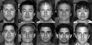
Figure 1: Some examples from the Yale Face Database B.

To compute the Affine-Invariant kernel (shown in Table I) on the Riemannian manifold, we use covariance descriptors [38] computed from the feature vector $\Big{[}x,y,I_{xy},|G_{x}|,|G_{y}|,\sqrt{G_{x}^{2}+G_{y}^{2}},|G_{xx}|,|G_{yy}|,\arctan\big{(}\frac{|G_{x}|}{|G_{y}|}\big{)}\Big{]}$, where $x$, $y$ are pixel locations, $I_{xy}$ is the grayscale value at $xy$-coordinate location, and $G_{x}$, $G_{y}$ are the first order intensity derivatives. Likewise, $G_{xx}$, $G_{yy}$ are the second order intensity derivatives. Accordingly, each face image in this database can be represented by the covariance matrix, i.e. a 9 $\times$ 9 SPD matrix. And then, the similarity between two images can be evaluated by the Affine-Invariant kernel.

TABLE V: Statistics of the Affine-Invariant(Aff-I) kernel and the test classification accuracy(%) on Yale Face Database B.

	$\mu_{\min}$	$\mu_{\max}$	SVM(Log-E)	KLR(Log-E)	Flip	Clip	Shift	TDCASVM	KSVM	CCICP-GD	CCICP-SGD
	-160.28	670.05	97.6$\pm$0.5	97.3$\pm$0.3	97.4$\pm$0.2	95.6$\pm$2.9	96.0$\pm$1.6	97.7$\pm$0.5	97.8$\pm$0.3	98.3$\pm$0.8	97.8$\pm$1.7

Table V presents statistics including the minimum and maximum eigenvalues of the Affine-Invariant kernel, i.e. $\mu_{\min}$ and $\mu_{\max}$. Note that such kernel on this data shows highly indefinite. We compare the proposed CCICP-GD and CCICP-SGD algorithms with five indefinite learning based methods with the Affine-Invariant kernel including “Flip”, “Clip”, “Shift”, “TDCASVM” and “KSVM”. And also, the Log-Euclidean kernel [16], a PD kernel, is incorporated into two representative classifiers SVM and KLR for comparisons. Table V reports the average test accuracy(%) across abovementioned algorithms. One can see that these kernel approximation based methods “Flip”, “Clip” and “Shift” do not achieve satisfactory performance when compared with other positive definite/indefinite kernel learning based algorithms. This is because the above methods actually change the indefinite matrix itself. Among these indefinite learning based algorithms, the proposed CCICP-GD algorithm performs better than “TDCASVM” and “KSVM” with a margin of 0.6% and 0.5% on the test classification accuracy. Besides, the proposed CCICP-SGD algorithm achieves a comparable performance among these methods. The experimental results on this data set reinforce to demonstrate the effectiveness of the proposed algorithms with various indefinite kernels.

V-D Effect of the Inexact Parameter $\epsilon$

As aforementioned, the only difference between CCCP-GD and CCICP-GD is the selection of the inexact parameter $\epsilon$. When $\epsilon$ approaches to zero, the CCICP-GD algorithm degenerates to a standard CCCP-GD algorithm. In our experiment, $\epsilon$ is set to 0.0001 in the CCCP-GD algorithm while we choose $\epsilon=1$ in CCICP-GD. Based on this, this section investigates how its variation (i.e. 0.0001, 0.001, 0.01, 0.1, 0.5, 1, 5) in the inexact solving scheme influences the test accuracy and the computational cost during training. Two data sets appeared in Section V-B are used here for our experiments, namely a small-scale data set monks1 and a larger one guide1-t.

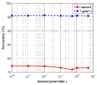
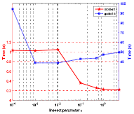
Figure 2: Influence of tuning $\epsilon$ on monks1 (red) and guide1-t (blue), with accuracy (a) and time (b) versus iteration.

Fig. 2 illustrates that the performance of CCICP-GD is generally not sensitive to $\epsilon$ on such two different types of data sets. In Fig. 2, on monks1, the training time cost does not dramatically decrease when $\epsilon$ ranges from 0.0001 to 0.01, and then it rapidly falls down. We can conclude that CCICP-GD ($\epsilon=\text{1}$) is much efficient than CCCP-GD ($\epsilon=\text{0.0001}$), and thus such tendency demonstrates the effectiveness of the proposed inexact scheme. Meanwhile, on guide1-t, the setting with $\epsilon=\text{0.001}$ spends the minimum time during training, which almost cuts by half when compared with the situation of initial value $\epsilon=\text{0.0001}$. After that, the time cost steadily increases, which shows an “abnormal” tendency on $\epsilon$. This is because the algorithm with an inexact solution sometimes requires more iterations to converge to a stationary point. However, CCICP-GD ($\epsilon=\text{1}$) is still efficient than CCCP-GD ($\epsilon=\text{0.0001}$) in this data set. Generally, CCICP-GD with larger $\epsilon$ often spends less training time than the setting with smaller one to converge. This is because the termination condition can be significantly relaxed, which has been well demonstrated on these two data sets.

V-E Algorithm Convergence

Fig. 3 shows the convergence of IKLR with three optimization algorithms on monks1 and ijcnn1-tr.

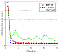
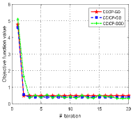
Figure 3: Convergence plots for CCCP-GD (red), CCICP-GD (blue) and CCICP-SGD (green) on monks1 (a) and ijcnn1-tr (b), respectively.

It can be observed that, in Fig. 3, on the monks1 data set, CCICP-GD converges within 5 iterations, but CCCP-GD takes 16 iterations to converge. In Fig. 3, both CCCP-GD and CCICP-GD converge fast on the ijcnn1-tr data set. The above two gradient-based algorithms (CCCP-GD and CCICP-GD) monotonically decrease in each iteration. However, in our CCICP-SGD version, it cannot be guaranteed to monotonically decrease due to its random scheme. Instead, it just converges to a stationary point in expectation as shown in Fig. 3.

V-F Different Random Initializations

TABLE VI: CCICP-GD and CCICP-SGD with different random initializations on the monks1 and guide1-t dataset.

Method	CCICP-GD		CCICP-SGD
Initialization	monks1	guide1-t	monks1	guide1-t
${\bm{\alpha}}^{(0)}=\bm{0}$	0.694	0.925	0.662$\pm$0.050	0.926$\pm$0.003
${\bm{\alpha}}^{(0)}=\bm{1}$	0.697	0.925	0.675$\pm$0.037	0.919$\pm$0.016
${\bm{\alpha}}^{(0)}=-\bm{1}$	0.694	0.925	0.661$\pm$0.043	0.923 $\pm$0.008
$\alpha^{(0)}_{i}\in(0,1)$	0.706	0.927	0.663$\pm$0.054	0.926$\pm$0.049

The proposed algorithms, CCICP-GD and CCICP-SGD, have been experimentally demonstrated to be converge as illustrated in Section V-E. Since the IKLR model is non-convex, different initializations might lead to different stationary points. Here we choose two data sets, monks1 and guide1-t, to investigate the influence of our algorithms with different initializations on the final classification accuracy. Such two data sets are conducted with 10 runs on a fixed (or pre-defined) training and test data for fair comparisons. As suggested in [41], in our experiment, we choose four different initializations with small values, i.e. ${\bm{\alpha}}^{(0)}=\bm{0}$, ${\bm{\alpha}}^{(0)}=\bm{1}$, ${\bm{\alpha}}^{(0)}=-\bm{1}$, and the randomly initialization $\alpha^{(0)}_{i}\in(0,1)$. By doing so, such small initialization values can guarantee that the objective function value in Eq. (6) is always positive during the optimization process. Table VI demonstrates that different initializations near zero often lead to slight fluctuation on the final classification accuracy.

V-G Discussion on CCICP-SGD

As aforementioned in Section V-A2, the inexact parameter $\epsilon$ in CCICP-SGD is fixed to 0.0001 because SGD achieves the similar purpose with the inexact scheme i.e., $\epsilon=\text{1}$. However, in Table IV, it can be observed that CCICP-GD is much efficient than CCICP-SGD. Such time cost reduction motivates us to see how fast our algorithm can be when SGD comes to the inexact scheme. Accordingly, we investigate the performance of CCICP-SGD with the early termination condition (i.e. $\epsilon=1$), termed as “CCICP-SGD-I”.

TABLE VII: Results of CCICP-SGD and CCICP-SGD-I on four larger than small scale data sets.

Dataset	EEG		guide1-t		ijcnn1-tr		madelon
Method	CCICP-SGD	CCICP-SGD-I	CCICP-SGD	CCICP-SGD-I	CCICP-SGD	CCICP-SGD-I	CCICP-SGD	CCICP-SGD-I
Accuracy	0.630$\pm$0.042	0.590$\pm$0.052	0.947$\pm$0.022	0.876$\pm$0.037	0.914$\pm$0.006	0.912$\pm$0.003	0.601$\pm$0.028	0.550$\pm$0.065
Training time	8776.4	71.2754	714.72	1.4146	28.23	2.445	160.71	2.543
Test time	0.1188	0.0235	0.0021	0.0023	0.2258	0.2378	0.0011	0.0025

Table VII reports the classification accuracy and the computation cost of CCICP-SGD and CCICP-SGD-I on four larger than small scale data sets. One can see that CCICP-SGD-I degrades the test accuracy to some extent when compared with CCICP-SGD on EEG, guide1-t, and madelon. However, CCICP-SGD-I equipped with the inexact scheme extremely accelerates the training process, of which the training time is about one-hundreds or less than that of CCICP-SGD. On ijcnn1-tr, CCICP-SGD-I is more efficient than CCICP-SGD without too much degeneracy on the classification accuracy.

VI Conclusion

In this paper, we investigate kernel logistic regression with indefinite kernels in theoretical and algorithmic aspects. The derived IKLR model is non-convex and further analysed in RKKS with explicit demonstration due to the non-positive definite kernels. Such non-convex problem can be effectively and efficiently solved by the proposed CCICP equipped with two approximation schemes. Its GD version using an early stop scheme is able to make the training process efficient; the stochastic variant of CCICP also has the capability of accelerating the solving process. The convergence analyses of CCICP-GD and CCICP-SGD are conducted with theoretical guarantees and experimental validation. The classification accuracy of the proposed IKLR model on several benchmarks demonstrates its effectiveness when compared to other positive definite/indefinite kernel learning methods.

References

- [1] Bernhard Schölkopf and Alexander J Smola, Learning with kernels: Support Vector Machines, Regularization, Optimization, and Beyond, MIT Press, 2003.
- [2] Vladimir N. Vapnik, The Nature of Statistical Learning Theory, Springer, 1995.
- [3] Ji Zhu and Trevor Hastie, “Kernel logistic regression and the import vector machine,” Journal of Computational and Graphical Statistics, vol. 14, no. 1, pp. 185–205, 2002.
- [4] Chen Gong, Dacheng Tao, Stephen J. Maybank, Wei Liu, Guoliang Kang, and Jie Yang, “Multi-modal curriculum learning for semi-supervised image classification,” IEEE Transactions on Image Processing, vol. 25, no. 7, pp. 3249–3260, 2016.
- [5] Harris Drucker, Christopher JC Burges, Linda Kaufman, Alex J Smola, and Vladimir Vapnik, “Support vector regression machines,” in Proceedings of Advances in neural information processing systems, 1997, pp. 155–161.
- [6] Inderjit S Dhillon, Yuqiang Guan, and Brian Kulis, “Kernel k-means: spectral clustering and normalized cuts,” in Proceedings of ACM SIGKDD international conference on Knowledge discovery and data mining. ACM, 2004, pp. 551–556.
- [7] Theodoros Evgeniou, Massimiliano Pontil, and Tomaso Poggio, “Regularization networks and support vector machines,” Advances in Computational Mathematics, vol. 13, no. 1, pp. 1–50, 2000.
- [8] Frank Michael Schleif and Peter Tino, “Indefinite proximity learning: A review,” Neural Computation, vol. 27, no. 10, pp. 2039–2096, 2015.
- [9] Hiroto Saigo, Jean Philippe Vert, Nobuhisa Ueda, and Tatsuya Akutsu, “Protein homology detection using string alignment kernels,” Bioinformatics, vol. 20, no. 11, pp. 1682–1689, 2004.
- [10] Nils M. Kriege, Pierre Louis Giscard, and Richard C. Wilson, “On valid optimal assignment kernels and applications to graph classification,” in Proceedings of Advances in Neural Information Processing Systems, 2016, pp. 1623–1631.
- [11] Eamonn Keogh and Chotirat Ann Ratanamahatana, “Exact indexing of dynamic time warping,” Knowledge and Information Systems, vol. 7, no. 3, pp. 358–386, 2005.
- [12] Pierre-Francois. Marteau and Sylvie Gibet, “On recursive edit distance kernels with application to time series classification.,” IEEE Transactions on Neural Networks and Learning Systems, vol. 26, no. 6, pp. 1121–1133, 2013.
- [13] Yiming Ying, Colin Campbell, and Mark Girolami, “Analysis of SVM with indefinite kernels,” in Proceedings of Advances in Neural Information Processing Systems, 2009, pp. 2205–2213.
- [14] Jianjia Zhang, Lei Wang, Luping Zhou, and Wanqing Li, “Learning discriminative stein kernel for SPD matrices and its applications,” IEEE Transactions on Neural Networks and Learning Systems, vol. 27, no. 5, pp. 1020–1033, 2015.
- [15] Chen Gong, Ting Liu, Dacheng Tao, Keren Fu, Enmei Tu, and Jie Yang, “Deformed graph laplacian for semisupervised learning,” IEEE Transactions on Neural Networks and Learning Systems, vol. 26, no. 10, pp. 2261–2274, 2015.
- [16] Sadeep Jayasumana, Richard Hartley, Mathieu Salzmann, Hongdong Li, and Mehrtash Harandi, “Kernel methods on the Riemannian manifold of symmetric positive definite matrices,” in Proceedings of the IEEE Conference on Computer Vision and Pattern Recognition, 2013, pp. 73–80.
- [17] Aasa Feragen, François Lauze, and Søren Hauberg, “Geodesic exponential kernels: When curvature and linearity conflict,” in Proceedings of the IEEE Conference on Computer Vision and Pattern Recognition, 2015, pp. 3032–3042.
- [18] Cheng Soon Ong, Xavier Mary, and Alexander J. Smola, “Learning with non-positive kernels,” in Proceedings of International Conference on Machine Learning, 2004, pp. 81–89.
- [19] Gaëlle Loosli, Stéphane Canu, and Soon Ong Cheng, “Learning SVM in Kreĭn spaces,” IEEE Transactions on Pattern Analysis and Machine Intelligence, vol. 38, no. 6, pp. 1204–1216, 2016.
- [20] Thore Graepel, Ralf Herbrich, Peter Bollmann-Sdorra, and Klaus Obermayer, “Classification on pairwise proximity data,” in Proceedings of Advances in Neural Information Processing Systems, 1999, vol. 11, pp. 438–444.
- [21] Elzbieta Pekalska, Pavel Paclik, and Robert P. W Duin, “A generalized kernel approach to dissimilarity-based classification,” Journal of Machine Learning Research, vol. 2, no. 2, pp. 175–211, 2002.
- [22] Volker Roth, Julian Laub, Motoaki Kawanabe, and Joachim Buhmann, “Optimal cluster preserving embedding of nonmetric proximity data,” IEEE Transactions on Pattern Analysis and Machine Intelligence, vol. 25, no. 12, pp. 1540–1551, 2003.
- [23] Chih-Chung Chang and Chih-Jen Lin, “LIBSVM: A library for support vector machines,” ACM Transactions on Intelligent Systems and Technology, vol. 2, pp. 27:1–27:27, 2011.
- [24] François Bertrand Akoa, “Combining DC algorithms (DCAs) and decomposition techniques for the training of nonpositive-semidefinite kernels,” IEEE Transactions on Neural Networks, vol. 19, no. 11, pp. 1854–1872, 2008.
- [25] Haiming Xu, Hui Xue, Xiaohong Chen, and Yunyun Wang, “Solving indefinite kernel support vector machine with difference of convex functions programming,” in Proceedings of AAAI Conference on Artificial Intelligence, 2017, pp. 1610–1616.
- [26] Alan L. Yuille and Anand Rangarajan, “The concave-convex procedure,” Neural Computation, vol. 15, no. 4, pp. 915–936, 2003.
- [27] Fanghui Liu, Xiaolin Huang, and Jie Yang, “Indefinite kernel logistic regression,” in Proceedings of the ACM Multimedia, 2017, pp. 846–853.
- [28] Bernhard Schölkopf, Ralf Herbrich, and Alex J Smola, “A generalized representer theorem,” in Proceedings of the Conference on Computational Learning Theory, 2000, pp. 416–426.
- [29] János Bognár, Indefinite inner product spaces, Springer, 1974.
- [30] Bernard Haasdonk, “Feature space interpretation of SVMs with indefinite kernels,” IEEE Transactions on Pattern Analysis and Machine Intelligence, vol. 27, no. 4, pp. 482–492, 2005.
- [31] Andrew Cotter, Ohad Shamir, Nathan Srebro, and Karthik Sridharan, “Better mini-batch algorithms via accelerated gradient methods,” in Proceedings of Advances in Neural Information Processing Systems, 2011, pp. 1647–1655.
- [32] Ioannis Mitliagkas, Constantine Caramanis, and Prateek Jain, “Memory limited, streaming PCA,” in Proceedings of Advances in Neural Information Processing Systems, 2013, pp. 2886–2894.
- [33] K Goebel and W. A Kirk, “A fixed point theorem for asymptotically nonexpansive mappings,” Proceedings of the American Mathematical Society, vol. 35, no. 1, pp. 171–174, 1972.
- [34] Guanghui Lan and Saeed Ghadimi, “Optimal stochastic approximation algorithms for strongly convex stochastic composite optimization, ii: Shrinking procedures and optimal algorithms,” SIAM Journal on Optimization, vol. 23, no. 4, pp. 2061–2089, 2010.
- [35] Atsushi Nitanda and Taiji Suzuki, “Stochastic difference of convex algorithm and its application to training deep boltzmann machines,” in Proceedings of Artificial Intelligence and Statistics, 2017, pp. 470–478.
- [36] Bharath K. Sriperumbudur and Gert R. G. Lanckriet, “On the convergence of the concave-convex procedure,” in Proceedings of the International Conference on Neural Information Processing Systems, 2009, pp. 1759–1767.
- [37] Xiaolin Huang, Johan A.K. Suykens, Shuning Wang, Joachim Hornegger, and Andreas Maier, “Classification with truncated distance kernel,” IEEE Transactions on Neural Networks and Learning Systems, vol. 29, no. 5, pp. 2025 – 2030, 2018.
- [38] Oncel Tuzel, Fatih Porikli, and Peter Meer, “Region covariance: A fast descriptor for detection and classification,” in Proceedings of the European Conference on Computer Vision, 2006, pp. 589–600.
- [39] Gang Wu, Edward Y Chang, and Zhihua Zhang, “An analysis of transformation on non-positive semidefinite similarity matrix for kernel machines,” Technical Report, 2005.
- [40] Catherine Blake and Christopher J. Merz, “UCI Repository of Machine Learning Databases,” 1998.
- [41] Yann Dauphin, Razvan Pascanu, Caglar Gulcehre, Kyunghyun Cho, Surya Ganguli, and Yoshua Bengio, “Identifying and attacking the saddle point problem in high-dimensional non-convex optimization,” in Proceedings of Neural Information Processing Systems, 2014, pp. 2933–2941.