Typical equilibrium state of an embedded quantum system

Abstract

We consider an arbitrary quantum system coupled non perturbatively to a large arbitrary and fully quantum environment. In [G. Ithier and F. Benaych-Georges, Phys. Rev. A 96, 012108 (2017)] the typicality of the dynamics of such an embedded quantum system was established for several classes of random interactions. In other words, the time evolution of its quantum state does not depend on the microscopic details of the interaction. Focusing at the long time regime, we use this property to calculate analytically a new partition function characterizing the stationary state and involving the overlaps between eigenvectors of a bare and a dressed Hamiltonian. This partition function provides a new thermodynamical ensemble which includes the microcanonical and canonical ensembles as particular cases. We check our predictions with numerical simulations.

In what state of equilibrium can a quantum system be? Does this state have universal properties and what are the conditions for its emergence? These questions are not new, dating even from the very birth of quantum theoryvonNeumann (1929) and are surprisingly openPolkovnikov et al. (2011); Eisert et al. (2015). Indeed, the foundations of statistical physics still rely today on a static Bayesian point of view assuming the equiprobability of the accessible states defining the microcanonical ensemble. Assuming temperature and chemical potential can be defined then the canonical and grand canonical ensembles can be derived, allowing to calculate all relevant macroscopic quantities in the thermodynamical limit Kubo et al. (1990); Landau and Lifschitz (1980); J. Gemmer (2004). In order to link theoretical predictions calculated with averages over these ensembles to experimental quantities measured on a single system, an assumption of ergodicity is made. Despite being broadly accepted, this assumption is not justified in a satisfactory manner (see, e.g., the discussion in Ref. Gemmer and Mahler (2003)). Triggered by recent progress in the quantum engineering of mesoscopic systems  Bloch et al. (2012); Devoret and Schoelkopf (2013), some theoretical progress has been achieved for attempting to explain thermodynamical equilibrium with a purely quantum point of view.

From the early work of von Neumann on quantum ergodicity vonNeumann (1929); Goldstein et al. (2010), most theoretical studies aiming at understanding thermalisation as a quantum and universal Uni process have focused on looking for signatures of thermalisation on physical observables of large quantum systems Deutsch (1991); Reimann (2015, 2007, 2016), for instance with the Eigenstate Thermalisation Hypothesis (ETH) surmise Srednicki (1994); Rigol et al. (2008); D’Alessio et al. (2016). Instead of observables, one can also focus on the state of a system embedded in a larger one for which a “canonical typicality” property has been established: the overwhelming majority of pure quantum states of the composite system are locallyLoc canonical Goldstein et al. (2006); Tasaki (1998); Popescu et al. (2006). This static “typicality” has been extended to the dynamics of embedded quantum systems (two-level Lebowitz J L and L , four-level Bratus and Pastur (2017) and arbitrary Ithier and Benaych-Georges (2017) quantum systems). We apply here this “dynamical typicality” property in order to calculate analytically and with full generality the stationary state of an embedded quantum system at long time. We find a new thermodynamical ensemble of purely quantum origin characterizing this state. This ensemble captures the microcanonical and the canonical ensembles as particular cases, and as such provides a quantum explanation for the Gibbs distribution.

We consider an arbitrary quantum system coupled to a large arbitrary quantum environment through a random interaction. We emphasize the fact that the initial state of this composite system can be chosen arbitrarily, in particular the environment does not have to be in thermal equilibrium initially nor the full composite system in the microcanonical situation. Dynamical typicality Lebowitz J L and L ; Ithier and Benaych-Georges (2017) states that for almost all interaction HamiltonianAlm the reduced density matrix of the system has a self-averaging property in the large environment limitPas , in other words, it follows a universal dynamics. Despite this does not imply a priori equilibration, since it can be consistent with sustained oscillations and revivalsCom , this property has a very practical consequence. It allows to perform non perturbative analytical calculations with full generality, i.e. for arbitrary system, environment, and global initial state, by justifying rigorously an averaging procedure over some randomness introduced only at the level of the interaction Hamiltonian. We apply this calculation framework here to study the state of the system at long but finite times, i.e. smaller than any recurrence time. Postponing all questions regarding the out of equilibrium dynamics to a further publication PLn , we show that: if the system converges towards a stationary state, then this state is characterized by a new quantum partition function which can be calculated. This partition function relies on an average transition probability between states involving some purely quantum quantities: the fourth order moments of the overlap coefficients between eigenvectors of a bare and a dressed Hamiltonian. We calculate this transition probability for several classes of random interactions. Then we calculate the probabilities of occupation of the states of the system a find a new thermodynamical ensemble more general than the microcanonical one.

Model Setup.— The setup is identical toIthier and Benaych-Georges (2017): we consider a system $S$ in contact with an environment $E$, writing $\mathcal{H}_{s}$, $\mathcal{H}_{e}$ for their respective Hilbert spaces. The total system $S+E$ is closed and its Hilbert space is the tensor product $\mathcal{H}=\mathcal{H}_{s}\otimes\mathcal{H}_{e}$ (with dimension $N=\dim\mathcal{H}_{e}.\dim\mathcal{H}_{s}$). The total or dressed Hamiltonian $\hat{H}$ is the sum $\hat{H}=\hat{H}_{s}+\hat{H}_{e}+\hat{W}$ where $\hat{W}$ is an interaction term. Eigenvectors of the “bare” Hamiltonian $\hat{H}_{s}+\hat{H}_{e}$ are written as $|\phi_{n}\rangle$ and are tensor products of eigenvectors $|\epsilon_{s}\rangle$ of $\hat{H}_{s}$ and eigenvectors $|\epsilon_{e}\rangle$ of $\hat{H}_{e}$, with the eigenenergy $\epsilon_{n}=\epsilon_{s}+\epsilon_{e}$. We write $|\psi_{i}\rangle$ for the dressed eigenvectors and $\{\lambda_{i}\}_{i}$ the set of associated dressed eigenvalues. The state of $S+E$ is described by a density matrix $\varrho(t)$ which follows the well known relation

$$\varrho(t)=\hat{U}_{t}\varrho(0)\hat{U}_{t}^{\dagger}\quad\text{with}\quad\hat{U}_{t}=e^{-\frac{i}{\hbar}\hat{H}t}.$$

The state of the subsystem $S$ is described by a reduced density matrix: $\varrho_{s}(t)=\operatorname{Tr}_{e}\varrho(t),$ $\operatorname{Tr}_{e}$ being the partial trace with respect to the environment. Decomposing the initial state $\varrho(0)$ on the bare eigenbasis $\{|\phi_{1}\rangle,..,|\phi_{N}\rangle\}$ and using linearity, we consider the matrix elements $\langle\phi_{n}|\hat{U}_{t}|\phi_{m}\rangle\langle\phi_{p}|\hat{U}^{\dagger}_{t}|\phi_{q}\rangle$ in order to calculate $\varrho_{s}(t)$. By expanding the evolution operator $\hat{U}_{t}$ over the dressed eigenbasis $\{|\psi_{1}\rangle,...,|\psi_{N}\rangle\}$: $\hat{U}_{t}=\sum_{i}e^{-\frac{i}{\hbar}\lambda_{i}t}|\psi_{i}\rangle\langle\psi_{i}|,$ these matrix elements can be re-written as the $2$ dimensional Fourier transform of a product of four “overlaps” $\langle\phi_{n}|\psi_{i}\rangle$:

$$\langle\phi_{n}|\hat{U}_{t}|\phi_{m}\rangle\langle\phi_{p}|\hat{U}_{t}^{\dagger}|\phi_{q}\rangle=\qquad\qquad\qquad\qquad\qquad$$

$$\sum_{i,j}e^{-\frac{i}{\hbar}(\lambda_{i}-\lambda_{j})t}\langle\phi_{n}|\psi_{i}\rangle\langle\psi_{i}|\phi_{m}\rangle\langle\phi_{p}|\psi_{j}\rangle\langle\psi_{j}|\phi_{q}\rangle.$$ (1)

To calculate the expression in Eq. (Typical equilibrium state of an embedded quantum system), one needs an analytical formula for the overlap coefficients $\langle\psi_{i}|\phi_{n}\rangle$ and the dressed eigenvalues $\lambda_{i}$, which are quantities usually accessible in a perturbative framework only. In this Letter, we use a statistical method for calculating these quantities in a non perturbative setting and for arbitrary system and environment.

Introducing randomness.— The method relies on the hypothesis assumed for the interaction Hamiltonian: we introduce deliberately some randomness in and only in the interaction $\hat{W}$ in order to perform calculations, knowing that this randomness actually will not matter in the large dimensionality limit ($\dim\mathcal{H}_{e}\to\infty$) due to the typicality of the dynamics Ithier and Benaych-Georges (2017). This randomness should be compatible with some macroscopic constraints: $\hat{W}$ “centered” i.e. $\operatorname{Tr}(\hat{W})=0$ and with fixed spectrum variance $\sigma_{w}^{2}=\operatorname{Tr}(\hat{W}.\hat{W}^{\dagger})/N$ independent of $N$. Then regarding the symmetry class of the randomness, we will assume $\hat{W}$ to be either a Wigner band random matrix (WBRM)WBR or a randomly rotated matrix (RRM i.e. of the type $\hat{U}.\hat{Q}.\hat{U}^{\dagger}$ with $\hat{Q}$ real diagonal fixed and $\hat{U}$ unitary or orthogonal Haar distributed). The WBRM ensembles are convenient for modeling interactions in heavy atoms and nucleiFlambaum et al. (1994); Fyodorov et al. (1996); Borgonovi et al. (2016). The sparsity of WBRM comes from the finite energy range of the interaction. On the other hand, RRM ensembles are dense, which contradicts the a priori two body nature of the interaction, but provides a convenient way for modeling the local spectral statistics of more physical interaction HamiltoniansPorter (1965); Brody et al. (1981); Mehta (1991); Ericson (1960); Borgonovi et al. (2016).

Then we focus on the reduced density matrix: $\varrho_{s}(t)=\operatorname{Tr}_{e}\varrho(t)$ and consider it as a function of the interaction $\hat{W}$, keeping all other parameters constant (time, spectra of $S$ and $E$, initial state). From Ithier and Benaych-Georges (2017), we know that this function undergoes for the random matrix ensembles considered, a phenomenon known as the “concentration of measure”Talagrand (1996): as $\dim\mathcal{H}_{e}\to\infty$, $\varrho_{s}(t)$ is getting very close to its mean value which provides the typical dynamics. Consequently, we can compute an approximate $\varrho_{s}(t)$ simply by averaging: $\varrho_{s}(t)=\operatorname{Tr}_{e}(\varrho(t))\approx\mathbb{E}[\operatorname{Tr}_{e}(\varrho(t))]=\operatorname{Tr}_{e}\left(\operatorname{\mathbb{E}}[\varrho(t)]\right)$, where $\mathbb{E}$ is the average over the set of interaction Hamiltonians considered. We are thus led to consider the average of Eq. (Typical equilibrium state of an embedded quantum system).

Statistics of the overlaps.— We will now focus specifically on the stationary regime at long times. Under the hypothesis assumed on the statistics of the interaction (WBRM and RRM ensembles) the dressed eigenvalues $\{\lambda_{1},...,\lambda_{N}\}$ undergo level repulsion and, as such, are non degenerate. This implies that the time independent terms are provided by the case $i=j$ in the summation in Eq.(Typical equilibrium state of an embedded quantum system) averaged over $\hat{W}$:

$$\sum_{i}\operatorname{\mathbb{E}}[\langle\phi_{n}|\psi_{i}\rangle\langle\psi_{i}|\phi_{m}\rangle\langle\phi_{p}|\psi_{i}\rangle\langle\psi_{i}|\phi_{q}\rangle].$$ (2)

The time dependent regime (given by the summation over $i$ and $j$ such that $i\neq j$) is outside the scope of this article. We will assume this regime to be damped (see Genway et al. (2013) for $\hat{W}$ in the WRBM ensemble), without revivalsCom at least on the largest time scale of this model ($1/D$ where $D$ is the mean level spacing of the dressed Hamiltonian) such that considering a stationary regime is meaningful over this time scale.

We first single out the non zero cases for the fourth order moments of the overlap coefficients: $\operatorname{\mathbb{E}}[\langle\phi_{n}|\psi_{i}\rangle\langle\psi_{i}|\phi_{m}\rangle\langle\phi_{p}|\psi_{i}\rangle\langle\psi_{i}|\phi_{q}\rangle]$ which are when ($n=m$ and $p=q$) or when ($n=q\text{ and }m=p$) Sup . The former case is involved in the asymptotic value of the off-diagonal terms of $\varrho_{s}(t)$ i.e. the quantum coherences of the state of $S$, which can be shown to be zero as expected in the limit $t\to\infty$ Sup . In the following, we focus on the later case ($n=q\text{ and }m=p$) which governs the dynamics of the diagonal terms of $\varrho(t)$ and $\varrho_{s}(t)$, i.e. the probabilities of occupation.

Average transition probability.— We define from Eq.(2) with $n=q$ and $m=p$, an average transition probability $\bar{p}_{m\to n}$ from an initial state $|\phi_{m}\rangle$ at $t=0$ to a final state $|\phi_{n}\rangle$ at $t\to\infty$:

$$\bar{p}_{m\to n}=\sum_{i}\operatorname{\mathbb{E}}[|\langle\phi_{n}|\psi_{i}\rangle|^{2}|\langle\phi_{m}|\psi_{i}\rangle|^{2}].$$ (3)

Such sum provides quantitatively how $|\phi_{n}\rangle$ is accessible from $|\phi_{m}\rangle$ and has been considered, e.g., numerically in the context of random two body interactions (TBRI) ensembles Flambaum et al. (1996) and analytically for some specific systems: quantum walkersKrapivsky et al. (2015); Luck (2016); JML . The particular case $m=n$ provides the return probability whose reciprocal $1/\bar{p}_{n\to n}$ is the so-called purity Linden et al. (2009, 2010); Short (2011); Ikeda and Ueda (2015). The leading order of $\bar{p}_{m\to n}$ is given by $\sum_{i}\operatorname{\mathbb{E}}[|\langle\phi_{n}|\psi_{i}\rangle|^{2}]\operatorname{\mathbb{E}}[|\langle\phi_{m}|\psi_{i}\rangle|^{2}]$ and involves the second order moment of the overlaps $\operatorname{\mathbb{E}}[|\langle\phi_{n}|\psi_{i}\rangle|^{2}]$. This quantity, multiplied by $\rho$, is called the local density of states (LDOS) and quantifies how much a bare eigenvector is delocalized or hybridized with the dressed eigenbasis and has already been considered in various contexts (nuclear physicsBreit and Wigner (1936); Wigner (1955, 1957), molecular physicsRice (1933), atomic physicsFlambaum et al. (1994), thermalisationDeutsch (1991), quantum chaosFlambaum et al. (1994), financial data analysisAllez and Bouchaud (2014); Allez et al. (2014), see also the review in Borgonovi et al. (2016)) for various cases of $\hat{H}_{0}$ and $\hat{W}.$ It has the following typical shape:

$$\operatorname{\mathbb{E}}[|\langle\phi_{n}|\psi_{i}\rangle|^{2}]\approx\frac{f\left(\bar{\lambda}_{i}-\epsilon_{n}\right)}{\int\rho_{s+e}(\epsilon)f(\bar{\lambda}_{i}-\epsilon)d\epsilon}$$ (4)

where $\rho_{s+e}$ is the bare density of states, $\bar{\lambda}_{i}$ is the mean of the dressed eigenvalue $\lambda_{i}$ and $f$ is a function peaked around zero with a typical width $\Gamma$. The denominator is here for the purpose of normalisation. For most models of $\hat{H}_{0}$ and $\hat{W}$, the function $f$ is a Lorentzian reminiscent of the Breit-Wigner law with a generalized Fermi Golden rule rate $\Gamma=\pi\sigma_{w}^{2}\rho/N$, $\rho$ being the dressed density of states (see, e.g., Ref. Borgonovi et al. (2016)). Interestingly, such a Lorentzian shape has been shown to preclude thermalisation in closed quantum systems made of interacting particles as far as observables of these systems are concernedSantos et al. (2012); Torres-Herrera et al. (2014); Borgonovi et al. (2016). However, regarding the problem we are interested in: a quantum system coupled to a large environment, it is important to stress that this Lorentzian shape does not preclude thermalisation, as we observe numerically (see Fig.1) and as far as the state of this embedded system is concerned. This point is rather subtle and its explanation involves dynamical typicality (see Sup for a detailed discussion). Finally, we emphasize that the subsequent calculation can also be performed using other shapes (see Sup for details and a short review of possible LDOS). In particular, our derivation can be applied to a Gaussian LDOS, relevant if $\hat{W}$ if enforces a two body nature of the interaction (TBRI) Flambaum et al. (1996); Kota (2014).

Assuming the interaction to be non perturbative, i.e. the mean level spacing $D$ is much smaller than the width $\Gamma$ and consequently the bare eigenvector $|\phi_{m}\rangle$ is delocalized over several ($\approx\Gamma\rho$) dressed eigenvectors, then one can proceed further with the calculation of $\bar{p}_{m\to n}$ by using a continuous approximation for the summation ($\sum_{i}\leftrightarrow\int\rho(\lambda)d\lambda$). The transition probability is then given by:

$$\bar{p}_{m\to n}\approx\frac{g\left(\epsilon_{m}-\epsilon_{n}\right)}{\int\rho_{s+e}(\epsilon)g(\epsilon_{m}-\epsilon)d\epsilon}$$ (5)

where $g=f\ast f$ is the convolution of $f$ with itself and with a typical width $\Gamma^{\prime}$. For instance, if the LDOS is Lorentzian (resp. gaussian) then $g$ is also a Lorentzian (resp. gaussian) with a width $\Gamma^{\prime}=2\Gamma$ (resp. $\Gamma^{\prime}=\sqrt{2}\Gamma$). At this stage, one should note that Eq.(5) is in sharp contrast with the microcanonical hypothesis of equiprobability of the accessible states. We have performed numerical simulations for $\bar{p}_{m\to n}$ with $\hat{W}$ in the Gaussian orthogonal ensemble (GOE) and found a satisfactory agreement with our predictionSup .

Typical asymptotic state.— Finally, to perform the partial trace and get $\varrho_{s}(t)$, we recall the final state $|\phi_{n}\rangle=|\epsilon_{s}\rangle|\epsilon_{e}\rangle$ and sum Eq.(5) over $\epsilon_{e}$ using a continuous approximation: $\operatorname{Tr}_{e}=\sum_{\epsilon_{e}}\leftrightarrow\int d\epsilon\;\rho_{e}(\epsilon)$. This provides the main result of this paper: for an initial state $\varrho(0)=|\phi_{m}\rangle\langle\phi_{m}|$, the long time stationary state of $S$ is distributed according to

$$p_{\epsilon_{s}}=\lim_{t\to\infty}\langle\epsilon_{s}|\varrho_{s}(t)|\epsilon_{s}\rangle\approx\dfrac{\int\rho_{e}(\epsilon_{e})g\left(\epsilon_{m}-\epsilon_{s}-\epsilon_{e}\right)d\epsilon_{e}}{\int\rho_{e+s}(\epsilon)g(\epsilon_{m}-\epsilon)d\epsilon}.\qquad$$ (6)

The denominator is the convolution of the bare density of states by the transition probability $g$ which provides the effective number of bare states accessible from the initial $|\phi_{m}\rangle$. Such a quantity $\int\rho_{e+s}(\epsilon)g(\epsilon_{m}-\epsilon)d\epsilon$ enforces the normalization condition and can be considered as a new partition function. The numerator is the convolution of the environment density of states by the transition probability $g$ and provides the effective number of accessible states such that $S$ is in the state of energy $\epsilon_{s}$. The probability of occupancy is the ratio of these two numbers. Let us now consider the case of intermediate coupling.

Intermediate coupling.— A temperature can be defined by $\beta=\frac{1}{kT}=\frac{d\ln\rho_{e}}{d\epsilon}$. Assuming a good decoupling between the micro ($D=1/\rho$), meso ($\Gamma^{\prime}$) and macro ($kT$) energy scales: $D\ll\Gamma^{\prime}\ll kT$, and considering all energies $\epsilon_{n},\epsilon_{m}$ to be inside the bulk of the spectrum, then the function $g$ in Eq.(6) can be approximated by a Dirac function which is ”sampling” $\rho_{e}(\epsilon)$ at $\epsilon_{e}=\epsilon_{m}-\epsilon_{s}$ and simplifying Eq.(6) for

$$p_{\epsilon_{s}}\approx\frac{\rho_{e}(\epsilon_{m}-\epsilon_{s})}{\rho_{s+e}(\epsilon_{m})}.$$ (7)

We are recovering here the same prediction as the one resulting from a microcanonical ensemble defined locally in energy, i.e. by assuming the equiprobability of all bare eigenstates inside a small energy window centered around the initial energy $\epsilon_{m}$. This prediction is checked numerically on Fig. 1. It is important to stress that we recovered this prediction with a purely quantum point of view: from the geometrical relation between the eigenvectors of the bare and dressed Hamiltonians. Note that by assuming the environment to be macroscopic, i.e. $kT$ does not depend on energy on a wide range and consequently $\rho_{e}$ scales exponentially with energy, one can recover the canonical ensemble prediction following the usual derivationKubo et al. (1990):

$$p_{\epsilon_{s}}\approx\frac{\rho_{e}(\epsilon_{m}-\epsilon_{s})}{\rho_{s+e}(\epsilon_{m})}=\frac{\rho_{e}(\epsilon_{m})e^{-\beta\epsilon_{s}}}{\sum_{\epsilon_{s^{\prime}}}\rho_{e}(\epsilon_{m})e^{-\beta\epsilon_{s^{\prime}}}}\approx\frac{e^{-\beta\epsilon_{s}}}{Z_{\beta}}$$

with $Z_{\beta}=\sum_{\epsilon_{s}}e^{-\beta\epsilon_{s}}$ the canonical partition function. In other words, the Boltzmann distribution is a particular case of the more general distribution provided by Eq.(6) whose origin is quantum.

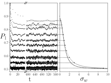
Figure 1: Crossover from a local microcanonical ensemble to a global microcanonical ensemble. We consider here numerically the particular case of a two level system $S$ (gap $\Delta=2$) coupled to an environment having a Gaussian density of states (standard deviation $\sigma_{e}=1$) through an interaction $\hat{W}$ in the GOE ensemble. We plot $P_{1}$ the probability for the system to be in its excited state as a function of time (left panel) and then the long time average of $P_{1}$ as a function of interaction strength $\sigma_{w}=\sqrt{\operatorname{Tr}(W^{2})/N}$ (right panel). The environment Hilbert space dimension is set to $\dim\mathcal{H}_{e}=4096$ (so that the total Hilbert space dimension is $N=8192$), the initial state to $|1_{s}\rangle\langle 1_{s}|\otimes|2048_{e}\rangle\langle 2048_{e}|$ (i.e. middle of the spectrum for $E$: $\epsilon_{e}\approx 0$) and we numerically integrate the Schrödinger equation for different values of $\sigma_{w}$. After a transient regime at short times ($t\lesssim 40$), a stationary regime takes place. As the interaction strength increases, the time average value of $P_{1}$ goes from a local microcanonical prediction $P_{1}\approx\rho_{e}(\Delta)/(\rho_{e}(\Delta)+\rho_{e}(0))\approx 0.87$ to a global microcanonical prediction: $P_{1}\approx 0.5$. The analytical prediction for this crossover (in dash) is given by Eq.(6) which can be calculated analytically in this case: it is the convolution of a gaussian DOS with a Lorentzian transition probability $g$ giving the Voigt functionVoigt (1912) (see Sup for details). Note that in the intermediate coupling regime, the LDOS (and consequently the average transition probability $\bar{p}_{m\to n}$) is of the Breit-Wigner type and does not preclude thermalization (see discussion in Sup for details).

Strong coupling.— If the coupling is strong enough that $\Gamma^{\prime}\gtrsim kT$ then the transition probability $g$ cannot be approximated by a Dirac function and its finite width must be taken into account in the convolution in Eq.(6). From this convolution effect, one should expect a decrease of contrast in the probability distribution of $S$ when the interaction strength is increased: the equilibrium probability then undergoes a continuous crossover from the local microcanonical ensemble prediction we described earlier (i.e. equiprobability over a small energy shell of accessible states around initial energy) to a global microcanonical ensemble prediction (i.e. all bare state are accessible and equiprobable). The convolution in Eq.(6) can be done analytically e.g. when $\rho_{e}$ is Gaussian and $g$ is Lorentzian: one obtains the Voigt distribution, relevant in atomic spectrocopy when a natural linewidth is broadened by the Doppler effectVoigt (1912). We check numerically these predictions on Fig. 1 and find a satisfactory agreement.

Finally, we stress that the above results are valid for an initial state $|\phi_{m}\rangle\otimes\langle\phi_{m}|=|\epsilon_{s}\rangle\langle\epsilon_{s}|\otimes|\epsilon_{e}\rangle\langle\epsilon_{e}|$ and can be extended by linearity to any initial state, pure or not: the extra diagonal terms (i.e. of the type $|\phi_{m}\rangle\langle\phi_{p}|$ with $m\neq p$) do not contributeSup , only the diagonal ones contribute. Therefore the stationary state of S is the weighted average of Eq. (6) by the initial energy distribution of the composite system.

Conclusion.— We showed that the stationary properties of an embedded quantum system are encoded in the geometric relation between the eigenvectors of a bare and a dressed Hamiltonian, more precisely in the fourth order moments of the overlaps between their eigenvectors. This fact provides a purely quantum way to define a new partition function which can be calculated thanks to dynamical typicalityIthier and Benaych-Georges (2017). In the intermediate coupling case $D\ll\Gamma^{\prime}\ll kT$, this partition function simplifies to the prediction of a local microcanonical ensemble defined on a small energy window around the initial energy. In the strong coupling regime (i.e. $D\ll kT\lesssim\Gamma^{\prime}$), one gets a more general ensemble which depends on the interaction strength and leads to a loss of contrast of the probabilities of occupation (i.e. a convergence towards global equiprobability). We considered here two random matrix ensembles for the interaction which have broad applicability. Our framework could be used with other interaction Hamiltonian ensembles (e.g. conserving some set of observables or enforcing the two body nature of the interaction) as soon as dynamical typicality is shown to be verified and a local density of states is available.

Acknowledgements.— We wish to thank D. Esteve and H. Grabert for their critical reading of the manuscript, their support and the numerous discussions, as well as J.-M. Luck, B. Cowan and X. Montiel for their useful comments and the discussions.

References

- vonNeumann (1929) J. vonNeumann, Z. Phys. , 30 (1929).
- Polkovnikov et al. (2011) A. Polkovnikov, K. Sengupta, A. Silva, and M. Vengalattore, Reviews of Modern Physics 83, 863 (2011).
- Eisert et al. (2015) J. Eisert, M. Friesdorf, and C. Gogolin, Nature Physics 11, 124 (2015).
- Kubo et al. (1990) R. Kubo, H. Ichimura, T. Usui, and N. Hashitsume, Statistical Mechanics (North Holland Personal Library, 1990).
- Landau and Lifschitz (1980) L. D. Landau and E. M. Lifschitz, Course of Theoretical Physics (Pergamon, Oxford, 1980).
- J. Gemmer (2004) G. M. J. Gemmer, M. Michel, Quantum Thermodynamics: Emergence of Thermodynamic Behavior within composite quantum systems, Lecture in Physics, Vol. 1200 (Springer, 2004).
- Gemmer and Mahler (2003) J. Gemmer and G. Mahler, The European Physical Journal B - Condensed Matter 31, 249 (2003), arXiv: quant-ph/0201136.
- Bloch et al. (2012) I. Bloch, J. Dalibard, and S. Nascimb ne, Nature Physics 8, 267 (2012).
- Devoret and Schoelkopf (2013) M. H. Devoret and R. J. Schoelkopf, Science 339, 1169 (2013).
- Goldstein et al. (2010) S. Goldstein, J. L. Lebowitz, C. Mastrodonato, R. Tumulka, and N. Zangh , Proceedings of the Royal Society of London A: Mathematical, Physical and Engineering Sciences 466, 3203 (2010).
- (11) By universal, we mean independent of the specific Hamiltonian considered.
- Deutsch (1991) J. M. Deutsch, Physical Review A 43, 2046 (1991).
- Reimann (2015) P. Reimann, New Journal of Physics 17, 055025 (2015).
- Reimann (2007) P. Reimann, Physical Review Letters 99, 160404 (2007).
- Reimann (2016) P. Reimann, Nature Communications 7, 10821 (2016).
- Srednicki (1994) M. Srednicki, Physical Review E 50, 888 (1994).
- Rigol et al. (2008) M. Rigol, V. Dunjko, and M. Olshanii, Nature 452, 854 (2008).
- D’Alessio et al. (2016) L. D’Alessio, Y. Kafri, A. Polkovnikov, and M. Rigol, Advances in Physics 65, 239 (2016).
- (19) By locally we mean after taking a partial trace to get the state of the subsystem.
- Goldstein et al. (2006) S. Goldstein, J. L. Lebowitz, R. Tumulka, and N. Zangh , Physical Review Letters 96, 050403 (2006).
- Tasaki (1998) H. Tasaki, Physical Review Letters 80, 1373 (1998).
- Popescu et al. (2006) S. Popescu, A. J. Short, and A. Winter, Nat Phys 2, 754 (2006).
- (23) L. A. Lebowitz J L and P. L, On a random matrix model of quantum relaxation., In: Contemporary Mathematics, “Adventures in Mathematical Physics”, Vol. 447 (F. Germinet, P. Hislop (Eds), AMS, Providence) pp. 199–218.
- Bratus and Pastur (2017) E. Bratus and L. Pastur, arXiv:1703.08209 [quant-ph] (2017), arXiv: 1703.08209.
- Ithier and Benaych-Georges (2017) G. Ithier and F. Benaych-Georges, Physical Review A 96, 012108 (2017).
- (26) This “almost all” is relative to the probability measure defined on the random matrix ensemble considered.
- (27) This self-averaging property was also used to investigate the local state of the microcanonical ensemble in the case of small subsystem and strong interactionLebowitz and Pastur (2015).
- (28) Because of the finite dimension of the Hilbert space, this regime might present quantum recurrences and revivals.
- (29) See Lebowitz and Pastur (2004); Lebowitz J L and L for the case of a two level system coupled to an environment through a separable random interaction.
- (30) WBRM are of the type where is a Wigner Random Matrix and is a deterministic band profile, “b” being the bandwidth.
- Flambaum et al. (1994) V. V. Flambaum, A. A. Gribakina, G. F. Gribakin, and M. G. Kozlov, Physical Review A 50, 267 (1994).
- Fyodorov et al. (1996) Y. V. Fyodorov, O. A. Chubykalo, F. M. Izrailev, and G. Casati, Physical Review Letters 76, 1603 (1996).
- Borgonovi et al. (2016) F. Borgonovi, F. M. Izrailev, L. F. Santos, and V. G. Zelevinsky, Physics Reports Quantum chaos and thermalization in isolated systems of interacting particles, 626, 1 (2016).
- Porter (1965) C. . Porter, Statistical Theories of Spectra: Fluctuations, edited by N. Y. Academy Press (1965).
- Brody et al. (1981) T. A. Brody, J. Flores, J. B. French, P. A. Mello, A. Pandey, and S. S. M. Wong, Reviews of Modern Physics 53, 385 (1981).
- Mehta (1991) M. L. Mehta, Random Matrices (Academic Press Inc, 1991).
- Ericson (1960) T. Ericson, Advances in Physics 9, 425 (1960).
- Talagrand (1996) M. Talagrand, Ann. Probab. 24, 1 (1996).
- Genway et al. (2013) S. Genway, A. F. Ho, and D. K. K. Lee, Physical Review Letters 111, 130408 (2013).
- (40) See Supplemental Material.
- Flambaum et al. (1996) V. V. Flambaum, G. F. Gribakin, and F. M. Izrailev, Physical Review E 53, 5729 (1996).
- Krapivsky et al. (2015) P. L. Krapivsky, J. M. Luck, and K. Mallick, Journal of Physics A: Mathematical and Theoretical 48, 475301 (2015).
- Luck (2016) J.-M. Luck, Journal of Physics A: Mathematical and Theoretical 49, 115303 (2016).
- (44) arXiv:1702.05909 .
- Linden et al. (2009) N. Linden, S. Popescu, A. J. Short, and A. Winter, Physical Review E 79, 061103 (2009).
- Linden et al. (2010) N. Linden, S. Popescu, A. J. Short, and A. Winter, New Journal of Physics 12, 055021 (2010).
- Short (2011) A. J. Short, New Journal of Physics 13, 053009 (2011).
- Ikeda and Ueda (2015) T. N. Ikeda and M. Ueda, Physical Review E 92, 020102 (2015).
- Breit and Wigner (1936) G. Breit and E. Wigner, Phys. Rev. 49, 519 (1936).
- Wigner (1955) E. P. Wigner, Annals of Mathematics 62, 548 (1955).
- Wigner (1957) E. P. Wigner, Annals of Mathematics 65, 203 (1957).
- Rice (1933) O. K. Rice, The Journal of Chemical Physics 1, 375 (1933).
- Allez and Bouchaud (2014) R. Allez and J.-P. Bouchaud, Random Matrices: Theory Appl. 03 (2014).
- Allez et al. (2014) R. Allez, J. Bun, and J.-P. Bouchaud, arXiv:1412.7108 [cond-mat] (2014), arXiv: 1412.7108.
- Santos et al. (2012) L. F. Santos, F. Borgonovi, and F. M. Izrailev, Physical Review Letters 108, 094102 (2012).
- Torres-Herrera et al. (2014) E. J. Torres-Herrera, M. Vyas, and L. F. Santos, New Journal of Physics 16, 063010 (2014).
- Kota (2014) V. K. B. Kota, Embedded Random Matrix Ensembles in Quantum Physics (Springer, 2014).
- Voigt (1912) W. Voigt, M unch. Ber. 603 (1912).
- Lebowitz and Pastur (2015) J. L. Lebowitz and L. Pastur, Journal of Physics A: Mathematical and Theoretical 48, 265201 (2015).
- Lebowitz and Pastur (2004) J. L. Lebowitz and L. Pastur, Journal Physics A: Mathematical and General 37, 1517 (2004).