Mode-Seeking Clustering and Density Ridge Estimation
via Direct Estimation of Density-Derivative-Ratios

Abstract

Modes and ridges of the probability density function behind observed data are useful geometric features. Mode-seeking clustering assigns cluster labels by associating data samples with the nearest modes, and estimation of density ridges enables us to find lower-dimensional structures hidden in data. A key technical challenge both in mode-seeking clustering and density ridge estimation is accurate estimation of the ratios of the first- and second-order density derivatives to the density. A naive approach takes a three-step approach of first estimating the data density, then computing its derivatives, and finally taking their ratios. However, this three-step approach can be unreliable because a good density estimator does not necessarily mean a good density derivative estimator, and division by the estimated density could significantly magnify the estimation error. To cope with these problems, we propose a novel estimator for the density-derivative-ratios. The proposed estimator does not involve density estimation, but rather directly approximates the ratios of density derivatives of any order. Moreover, we establish a convergence rate of the proposed estimator. Based on the proposed estimator, novel methods both for mode-seeking clustering and density ridge estimation are developed, and the respective convergence rates to the mode and ridge of the underlying density are also established. Finally, we experimentally demonstrate that the developed methods significantly outperform existing methods, particularly for relatively high-dimensional data.

1 Introduction

Characterizing the probability density function underlying observed data is a fundamental problem in machine learning. One approach is to consider geometric properties of the density such as modes and ridges. Estimation of such geometric properties is a challenging task, yet offers a variety of applications (Wasserman, 2018).

The modes (i.e., local maxima) of probability density functions have received much attention over the years. A motivation of estimating the modes classically appeared in the seminal work on kernel density estimation (Parzen, 1962). More recently, the modes of density functions for random curves have been used in functional data analysis (Gasser et al., 1998). Furthermore, in supervised learning, modal regression associates input variables with the modes of the conditional density function of the output variable, and enables us to simultaneously capture multiple functional relationships between the input and output (Sager and Thisted, 1982; Carreira-Perpiñán, 2000, 2001; Einbeck and Tutz, 2006; Chen et al., 2016a; Sasaki et al., 2016). One of the most natural applications is clustering. Mean shift clustering (MS) makes use of the modes of the estimated density function (Fukunaga and Hostetler, 1975; Cheng, 1995; Comaniciu and Meer, 2002): MS initially regards all data samples as candidates for cluster centers, and then iteratively updates them toward the nearest modes of the estimated density by gradient ascent (Fig.2). Finally, the data samples which converge to the same mode are assigned the same cluster label. Unlike standard clustering methods such as k-means clustering (MacQueen, 1967) and mixture-model-based clustering (Melnykov and Maitra, 2010), the notable advantage is that the number of clusters is automatically determined according to the number of detected modes. MS has been applied to a wide range of tasks such as image segmentation (Comaniciu and Meer, 2002; Tao et al., 2007; Wang et al., 2004) and object tracking (Collins, 2003; Comaniciu et al., 2000). (See also a recent review article by Carreira-Perpiñán (2015))

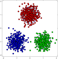
(a) Iteration=0

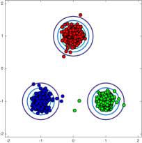
(b) Iteration=1

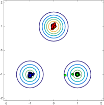
(c) Iteration=3

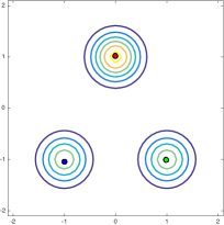
(d) Iteration=10

Figure 1: Illustration of a mode-seeking process. The contour plot indicates the probability density function that generates the data samples.

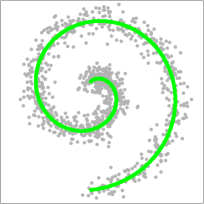
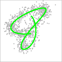
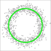
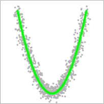
Figure 2: Examples of the density ridges hidden in data. Gray dot points and green curves indicate data samples and density ridges, respectively.

A ridge of the probability density function generalizes the notion of the mode. The density ridge is a lower-dimensional hidden structure of the data (Fig.2), and the zero-dimensional ridge can be interpreted as the mode (Genovese et al., 2014). Application of density ridge estimation can be found in a variety of fields such as filamentary structure estimation in cosmology (Chen et al., 2016c), extraction of curvilinear structures (e.g., blood vessels in the eyes) in medical imaging (You et al., 2011), and shape analysis in computer vision (Su et al., 2013) (See Pulkkinen (2015) for more applications). Density ridge estimation is closely related to manifold estimation. When data is assumed to be generated on a lower-dimensional manifold with additive Gaussian noise, density ridge estimation offers a way to circumvent the difficulty of manifold estimation: Genovese et al. (2014) theoretically proved that the density ridges capture the essential properties of such manifolds and estimating the density ridge is substantially easier than estimating the manifold. A practical algorithm called subspace constrained mean shift (SCMS) was proposed by Ozertem and Erdogmus (2011). SCMS is an extension to MS, but a projected gradient ascent method is performed to find density ridges instead of the gradient ascent method in MS; the gradient vector of the estimated density is projected to the subspace which is orthogonal to the ridge. Such a subspace can be obtained by applying principal component analysis to an estimate of the Hessian matrix of the log-density, which is composed of the ratios of the first- and second-order density derivatives to the density. Along the projected gradient vector, SCMS updates data points toward the ridge of the estimated density until convergence.

For MS, the technical challenge is accurate estimation of the derivatives of the probability density function. To derive practical methods, MS takes a two-step approach, firstly estimating the probability density function and then computing its derivatives (Comaniciu and Meer, 2002, Section 2). However, this approach can be unreliable because a good density estimator does not necessarily imply a good density derivative estimator in many practical situations. For example, small random fluctuations in a density estimate can create fake modes and may produce large errors in density-derivative estimation, even if the density estimate is fairly good in terms of density estimation (Genovese et al., 2016, Fig.1). Therefore, testing methods have been proposed to investigate whether the estimated modes are real modes from the underlying data density or fake modes due to the random fluctuations (Godtliebsen et al., 2002; Duong et al., 2008; Genovese et al., 2016). For SCMS, it is even more challenging to estimate the ratios of density derivatives to the density, but SCMS also naively estimates the ratios by adding one more step to the two-step approach in MS: the computed density derivatives are divided by the estimated density. However, such a division could strongly magnify estimation error.

To cope with these problems, we propose a novel estimator of the ratios of density derivatives to the density. In stark contrast with the approaches in MS and SCMS, the key idea is to directly estimate the ratios without going through density estimation. Moreover, we theoretically analyze the proposed estimator and establish a convergence rate. The direct approach has been adopted and proved to be useful both empirically and theoretically when estimating the ratio of two probability density functions (Sugiyama et al., 2008; Nguyen et al., 2008; Kanamori et al., 2009, 2012; Sugiyama et al., 2012; Kpotufe, 2017). Here, we follow the direct approach in the context of a different problem and derive an estimator in a substantially different way. Previously, a direct estimator has been proposed for the log-density derivatives (Beran, 1976; Cox, 1985), which are the ratios of first-order density derivatives to the density. On the other hand, the proposed estimator in this paper approximates the ratio of the derivatives of any order to the density, and thus generalizes the previous estimator.

The proposed estimator is first applied to mode-seeking clustering. We derive an update rule for mode-seeking based on a fixed-point algorithm, while inheriting the advantage of MS: the proposed clustering method also does not require the number of clusters to be specified in advance. This is advantageous because clustering is an unsupervised learning problem and tuning the number of clusters is not straightforward in general. Next, based on the mode-seeking clustering, we propose a novel method for density ridge estimation. For both methods, we prove the consistency of the mode and ridge estimators, and establish the convergence rates. Finally, we experimentally demonstrate that our proposed methods outperform MS and SCMS, particularly for high(er)-dimensional data.

This paper is organized as follows: In Section 2, we propose a novel estimator for the ratio of the derivatives of any order to the density, and establish a non-parametric convergence rate. The proposed estimator is applied to develop novel methods for mode-seeking clustering and density ridge estimation in Sections 3 and 4 respectively, and both methods are theoretically analyzed. Section 5 experimentally investigates the performance of the proposed methods for mode-seeking clustering and density ridge estimation. Section 6 concludes this paper. Preliminary results of this paper were presented at ECML/PKDD 2014 (Sasaki et al., 2014) and AISTATS 2017 (Sasaki et al., 2017). However, in addition to combining the results in those conference papers, we have added new theoretical analysis of the proposed estimator, mode-seeking clustering and density ridge estimation methods. From a theoretical stand point, we further improved upon the methods appeared in the conference papers, and performed more experiments in this paper.

2 Direct Estimation of Density-Derivative-Ratios

This section proposes a novel estimator of the ratios of density derivatives to the density and performs theoretical analysis.

2.1 Problem Formulation

Suppose that $n$ i.i.d. samples, which were drawn from a probability distribution on $\mathbb{R}^{D}$ with density $p(\bm{x})$, are available:

$$\mathcal{D}:=\{\bm{x}_{i}=(x_{i}^{(1)},x_{i}^{(2)},\dots,x_{i}^{(D)})^{\top}\}_{i=1}^{n}\overset{\text{i.i.d.}}{\sim}p(\bm{x}).$$

Here, our goal is to estimate the ratio of the $|\bm{j}|$-th order partial derivative of $p(\bm{x})$ to $p(\bm{x})$ from $\mathcal{D}=\{\bm{x}_{i}\}_{i=1}^{n}$,

$$\frac{\partial_{\bm{j}}p(\bm{x})}{p(\bm{x})},$$ (1)

where $\partial_{\bm{j}}=\frac{\partial^{|\bm{j}|}}{\partial^{j_{1}}x^{(1)}\partial^{j_{2}}x^{(2)}\dots\partial^{j_{D}}x^{(D)}}$, $\bm{j}=(j_{1},j_{2},\dots,j_{D})^{\top}$ and $|\bm{j}|=j_{1}+j_{2}+\dots+j_{D}$ for non-negative integers $j_{i}=0,1,\dots,|\bm{j}|$. For instance, when $|\bm{j}|=1$ (or $|\bm{j}|=2$), $\partial_{\bm{j}}p(\bm{x})/p(\bm{x})$ is a single element of $\nabla p(\bm{x})/p(\bm{x})$ (or of $\nabla\nabla p(\bm{x})/p(\bm{x})$).

2.2 Least-Squares Density-Derivative-Ratios

Our main idea is to directly fit a model $r_{\bm{j}}(\bm{x})$ to $\partial_{\bm{j}}p(\bm{x})/p(\bm{x})$ under the squared-loss:

$$J_{\bm{j}}(r_{\bm{j}}) :=\int\left\{r_{\bm{j}}(\bm{x})-\frac{\partial_{\bm{j}}p(\bm{x})}{p(\bm{x})}\right\}^{2}p(\bm{x})\mathrm{d}\bm{x}$$

$$=\int\left\{r_{\bm{j}}(\bm{x})\right\}^{2}p(\bm{x})\mathrm{d}\bm{x}-2\int r_{\bm{j}}(\bm{x})\partial_{\bm{j}}p(\bm{x})\mathrm{d}\bm{x}+\int\left\{\frac{\partial_{\bm{j}}p(\bm{x})}{p(\bm{x})}\right\}^{2}p(\bm{x})\mathrm{d}\bm{x}.$$ (2)

The first term on the right-hand side of (2) can be naively estimated from samples and the third term is ignorable, but it seems challenging to estimate the second term because it includes the derivative of the unknown density. However, as in Sasaki et al. (2015), repeatedly applying integration by parts allows us to transform the second term as

$$\int r_{\bm{j}}(\bm{x})\left\{\partial_{\bm{j}}p(\bm{x})\right\}\mathrm{d}\bm{x} =(-1)^{|\bm{j}|}\int\left\{\partial_{\bm{j}}r_{\bm{j}}(\bm{x})\right\}p(\bm{x})\mathrm{d}\bm{x},$$ (3)

where we assumed that as $|x^{(j)}|\rightarrow\infty$ for all $j$, the product of $\partial_{\bm{j}_{1}}r_{\bm{j}}(\bm{x})$ and $\partial_{\bm{j}_{2}}p(\bm{x})$ approaches zero for any pairs of $\bm{j}_{1}$ and $\bm{j}_{2}$ satisfying $|\bm{j}_{1}|+|\bm{j}_{2}|=|\bm{j}|-1$ for $|\bm{j}_{1}|,|\bm{j}_{2}|=0,1,\dots,|\bm{j}|-1$. As a result, the right-hand side of (3) can be easily estimated from samples. Then, an empirical version of (2) is given by

$$\widehat{J}_{\bm{j}}(r_{\bm{j}}):=\frac{1}{n}\sum_{i=1}^{n}\left\{r_{\bm{j}}(\bm{x}_{i})^{2}-2(-1)^{|\bm{j}|}\partial_{\bm{j}}r_{\bm{j}}(\bm{x}_{i})\right\}+\text{const.}$$ (4)

After adding the regularizer $R(r_{\bm{j}})$, the estimator is defined as the minimizer of

$$\widehat{r}_{\bm{j}}:=\mathop{\rm argmin}\limits_{r_{\bm{j}}}\left[\widehat{J}_{\bm{j}}(r_{\bm{j}})+\lambda_{\bm{j}}R(r_{\bm{j}})\right],$$ (5)

where $\lambda_{\bm{j}}$ is the regularization parameter.

We call this method the least-squares density-derivative ratios (LSDDR). Note that when $|\bm{j}|=1$, $J_{\bm{j}}$ is called the Fisher divergence and has been used for parameter estimation of unnnormalized statistical models (Hyvärinen, 2005), density estimation with the computationally intractable partition function (Sriperumbudur et al., 2017), and direct estimation of log-density derivatives (Beran, 1976; Cox, 1985; Sasaki et al., 2014). Therefore, LSDDR can be regarded as a generalization of such methods to higher-order derivatives.

2.3 Theoretical Analysis of LSDDR

Next, we theoretically analyze LSDDR.

2.3.1 Preliminaries and Notations

For a $D$-dimensional vector $\bm{x}\in\mathbb{R}^{D}$, the norm is defined by $\|\bm{x}\|:=\sqrt{\sum_{j=1}^{D}(x^{(j)})^{2}}$. For a domain $\mathcal{X}(\subseteq\mathbb{R}^{D})$, $C(\mathcal{X})$ denotes the space of all continuous functions on $\mathcal{X}$. Furthermore, we define the $L^{p}$ space of functions $f$ on $\mathcal{X}$: For $1\leq p\leq\infty$, $L^{p}(\mathcal{X}):=\{f~{}:~{}\|f\|_{p}<\infty\}$ where $\|\cdot\|_{p}$ is the $L^{p}$ norm defined by $\|f\|_{p}:=\left(\int|f(\bm{x})|^{p}\mathrm{d}\bm{x}\right)^{\frac{1}{p}}$ with the Lebesgue measure for $1\leq p<\infty$ and $\|f\|_{\infty}:=\mathop{\rm ess~{}sup}_{\bm{x}\in\mathcal{X}}|f(\bm{x})|$. For $f\in L^{1}(\mathbb{R}^{D})$, the Fourier transform is defined as

$$f^{\wedge}(\bm{\omega}):=\frac{1}{(2\pi)^{D/2}}\int f(\bm{x})e^{-i\bm{\omega}^{\top}\bm{x}}\mathrm{d}\bm{x},$$

where $i$ denotes the imaginary unit.

Let $\mathcal{H}$ be a reproducing kernel Hilbert space (RKHS) over $\mathcal{X}$ uniquely associated with the reproducing kernel $k:\mathcal{X}\times\mathcal{X}\rightarrow\mathbb{R}$. The norm and inner product on $\mathcal{H}$ are denoted by $\|\cdot\|_{\mathcal{H}}$ and $\langle\cdot,\cdot\rangle_{\mathcal{H}}$, respectively. $k$ is a real-valued, symmetric and positive definite function and has the reproducing property: For all $\bm{x}\in\mathcal{X}$ and $f\in\mathcal{H}$, $\langle f,k(\cdot,\bm{x})\rangle_{\mathcal{H}}=f(\bm{x})$. An example of reproducing kernels is the Gaussian kernel, $k(\bm{x},\bm{y})=\exp\left(-\frac{\|\bm{x}-\bm{y}\|^{2}}{2\sigma^{2}}\right)$ where $\sigma>0$ is the width parameter. Another example is the Matérn kernel, $k(\bm{x},\bm{y})=\psi(\bm{x}-\bm{y})=\frac{2^{1-s}}{\Gamma(s)}\|\bm{x}-\bm{y}\|^{s-D/2}\mathfrak{K}_{D/2-s}(\|\bm{x}-\bm{y}\|)$, whose corresponding RKHS $\mathcal{H}$ coincides with the Sobolev space $H^{s}_{2}$ with the smoothness parameter $s>D/2$ (Wendland, 2004, Chapter 10):

$$\mathcal{H}=H^{s}_{2}:=\left\{f\in L^{2}(\mathbb{R}^{D})\cap C(\mathbb{R}^{D}):\int(1+\|\bm{\omega}\|^{2})^{s}|f^{\wedge}(\bm{\omega})|^{2}\mathrm{d}\bm{\omega}<\infty\right\}.$$

$\Gamma(\cdot)$ denotes the Gamma function, and $\mathfrak{K}_{v}(\cdot)$ is the modified Bessel function of the second kind of order $v$.

2.3.2 The Convergence Rate of LSDDR

Here, we derive a rate of convergence for LSDDR under the RKHS norm. To this end, we assume that the true density-derivative-ratio is contained in $\mathcal{H}$:

$$r^{*}_{\bm{j}}(\bm{x}):=\frac{\partial_{\bm{j}}p(\bm{x})}{p(\bm{x})}\in\mathcal{H}.$$

Furthermore, we restrict the search space of $r_{\bm{j}}$ to $\mathcal{H}$ and express LSDDR with $R(r_{\bm{j}})=\|r_{\bm{j}}\|_{\mathcal{H}}^{2}$ as

$$\widehat{r}_{\bm{j}}=\mathop{\rm argmin}\limits_{r_{\bm{j}}\in\mathcal{H}}\left[\widehat{J}_{\bm{j}}(r_{\bm{j}})+\lambda_{\bm{j}}\|r_{\bm{j}}\|_{\mathcal{H}}^{2}\right].$$ (6)

To establish a convergence rate under the RKHS norm, we make the following assumptions as in Sriperumbudur et al. (2013):

• $\mathcal{X}$ is compact.

• $k$ is $2|\bm{j}|$ continuously differentiable.

• The following equation holds:

  $$\int_{\mathcal{X}}k(\cdot,\bm{x})\partial_{\bm{j}}p(\bm{x})\mathrm{d}\bm{x}=(-1)^{|\bm{j}|}\int_{\mathcal{X}}\partial_{\bm{j}}k(\cdot,\bm{x})p(\bm{x})\mathrm{d}\bm{x}.$$

• For all $\bm{j}$, there exists $\epsilon\geq 1$ subject to

  $$\left(\int_{\mathcal{X}}\|k(\cdot,\bm{x})\|_{\mathcal{H}}^{2\epsilon}p(\bm{x})\mathrm{d}\bm{x}\right)^{\frac{1}{2\epsilon}}<\infty\quad\text{and}\quad\left(\int_{\mathcal{X}}\|\partial_{\bm{j}}k(\cdot,\bm{x})\|_{\mathcal{H}}^{\epsilon}p(\bm{x})\mathrm{d}\bm{x}\right)^{\frac{1}{\epsilon}}<\infty.$$

Assumption (A) makes $\mathcal{H}$ separable (Steinwart and Christmann, 2008, Lemma 4.33) and the separability of $\mathcal{H}$ is required to apply Proposition A.2 in Sriperumbudur et al. (2013). Assumption (B) ensures that arbitrary functions in $\mathcal{H}$ are $2|\bm{j}|$ continuously differentiable (Steinwart and Christmann, 2008, Corollary 4.36). Assumption (C) holds under mild assumptions of $k$ and $p$ as in (3). From Assumption (D), $J_{\bm{j}}(r_{\bm{j}})<\infty$ when $\epsilon=1$. Then, the following theorem establishes the convergence rate under the RKHS norm:

Theorem 1

Let

$$C:=\int_{\mathcal{X}}k(\cdot,\bm{x})\otimes k(\cdot,\bm{x})p(\bm{x})\mathrm{d}\bm{x},$$

where $\otimes$ denotes the tensor product, be an operator on $\mathcal{H}$. If there exists $\gamma>0$ such that $r^{*}_{\bm{j}}$ is in the range of $C^{\gamma}$ (i.e., $r^{*}_{\bm{j}}\in\mathcal{R}(C^{\gamma})$), then

$$\|\widehat{r}_{\bm{j}}-r^{*}_{\bm{j}}\|_{\mathcal{H}}=O_{\mathrm{P}}\left(n^{-\min\left\{\frac{1}{4},\frac{\gamma}{2(\gamma+1)}\right\}}\right),$$

with $\epsilon=2$ and $\lambda_{\bm{j}}=O\left(n^{-\max\left\{\frac{1}{4},\frac{1}{2(\gamma+1)}\right\}}\right)$ as $n\rightarrow\infty$.

The proof is given in Appendix A. We followed the proof techniques in Sriperumbudur et al. (2013), but adopted them to a different problem: Sriperumbudur et al. (2013) proposed and analyzed a non-parametric estimator for log-densities with the intractable partition functions based on the Fisher divergence, which is a special case of $J_{\bm{j}}$ at $|\bm{j}|=1$. The range space assumption $r^{*}_{\bm{j}}\in\mathcal{R}(C^{\gamma})$ is closely related to the smoothness of $r^{*}_{\bm{j}}$ (Sriperumbudur et al., 2013, Section 4.2): Larger $\gamma$ implies that $r^{*}_{\bm{j}}$ is smoother. As seen in Sections 3.3.3 and 4.3.2, Theorem 1 is particularly useful in the analysis of our mode-seeking clustering and density ridge estimation methods.

Remark 2

By following Sriperumbudur et al. (2017, Section 4.2), Theorem 1 has some connection to the minimax theory (Tsybakov, 2009) under Sobolev spaces where for any $\alpha>s\geq 0$, the minimax rate is given by

$$\inf_{\widehat{r}_{\bm{j},n}}\sup_{r_{\bm{j}}^{*}\in H^{\alpha}_{2}}\|\widehat{r}_{\bm{j},n}-r_{\bm{j}}^{*}\|_{H^{s}_{2}}\asymp n^{-\frac{\alpha-s}{2(\alpha-s)+D}}.$$

$\inf$ is taken over possible estimators $\widehat{r}_{\bm{j},n}$, and $a_{n}\asymp b_{n}$ means that $a_{n}/b_{n}$ has lower- and upper-bounds away from zero and infinity, respectively. To establish a connection to Sobolev spaces, suppose that the Matérn kernel is employed whose corresponding RKHS is a Sobolev space $\mathcal{H}=H^{s}_{2}$ with the smoothness parameter $s>D/2$. As proved in Appendix B, when the true density belongs to $L^{1}(\mathbb{R}^{D})$ (i.e., $p\in L^{1}(\mathbb{R}^{D})$), $r^{*}_{\bm{j}}\in\mathcal{R}(C^{\gamma})$ for $\gamma\geq 1$ implies that $r^{*}_{\bm{j}}\in H^{\frac{3D}{2}-\frac{1}{2}+\epsilon}_{2}$ for arbitrarily small $\epsilon>0$. Then, the convergence rate $n^{-\frac{1}{4}}$ is minimax optimal under $\mathcal{H}=H^{D-\frac{1}{2}+\epsilon}_{2}$. Furthermore, this result implies that the dimension effect is veiled through the relative smoothness between two Sobolev spaces ($H^{\frac{3D}{2}-\frac{1}{2}+\epsilon}_{2}$ and $H^{D-\frac{1}{2}+\epsilon}_{2}$), and therefore the rate in Theorem 1 is independent of data dimension $D$. Details are provided in Appendix B.

2.4 Practical Implementation of LSDDR

Here, we describe practical implementation of LSDDR.

• A practical version of LSDDR: The representer theorem (Zhou, 2008, Theorem 2) states that the estimator $\widehat{r}_{\bm{j}}$ should take the following form:

  $$\widehat{r}_{\bm{j}}(\bm{x})=\sum_{i=1}^{n}\alpha^{(i)}_{\bm{j}}k(\bm{x},\bm{x}_{i})+\beta^{(i)}_{\bm{j}}\partial_{\bm{j}}^{\prime}k(\bm{x},\bm{x}^{\prime})\Bigr{|}_{\bm{x}^{\prime}=\bm{x}_{i}}=\sum_{i=1}^{2n}\theta^{(i)}_{\bm{j}}\psi_{\bm{j}}^{(i)}(\bm{x})=\bm{\theta}_{\bm{j}}^{\top}\bm{\psi}_{\bm{j}}(\bm{x}),$$ (7)

  where $\partial_{\bm{j}}^{\prime}$ denotes the partial derivative with respect to $\bm{x}^{\prime}$,

  $$\theta^{(i)}_{\bm{j}}:=\left\{\begin{array}[]{ll}\alpha^{(i)}_{\bm{j}}&i=1,\dots,n,\\ \beta^{(i-n)}_{\bm{j}}&i=n+1,\dots,2n,\end{array}\right.\qquad\psi_{\bm{j}}^{(i)}(\bm{x}):=\left\{\begin{array}[]{ll}k(\bm{x},\bm{x}_{i})&i=1,\dots,n,\\ \partial_{\bm{j}}^{\prime}k(\bm{x},\bm{x}^{\prime})\Bigr{|}_{\bm{x}^{\prime}=\bm{x}_{i-n}}&i=n+1,\dots,2n.\end{array}\right.$$

  To estimate $\bm{\theta}_{\bm{j}}$, we substitute (7) into $\widehat{J}_{\bm{j}}$ in (4). Then, when $R(r_{\bm{j}})=\bm{\theta}_{\bm{j}}^{\top}\bm{\theta}_{\bm{j}}$, the optimal solution of $\bm{\theta}_{\bm{j}}$ can be computed analytically as

  $$\widehat{\bm{\theta}}_{\bm{j}} :=\mathop{\rm argmin}\limits_{\bm{\theta}_{\bm{j}}}\left[\bm{\theta}_{\bm{j}}^{\top}\widehat{\bm{G}}_{\bm{j}}\bm{\theta}_{\bm{j}}-2(-1)^{|\bm{j}|}\bm{\theta}_{\bm{j}}^{\top}\widehat{\bm{h}}_{\bm{j}}+\lambda_{\bm{j}}\bm{\theta}_{\bm{j}}^{\top}\bm{\theta}_{\bm{j}}\right]=(-1)^{|\bm{j}|}\left(\widehat{\bm{G}}_{\bm{j}}+\lambda_{\bm{j}}\mathbf{I}_{2n}\right)^{-1}\widehat{\bm{h}}_{\bm{j}},$$

  where $\mathbf{I}_{2n}$ denotes the $2n$ by $2n$ identity matrix,

  $$\widehat{\bm{G}}_{\bm{j}}:=\frac{1}{n}\sum_{i=1}^{n}\bm{\psi}_{\bm{j}}(\bm{x}_{i})\bm{\psi}_{\bm{j}}(\bm{x}_{i})^{\top}\qquad\text{and}\qquad\widehat{\bm{h}}_{\bm{j}} :=\frac{1}{n}\sum_{i=1}^{n}\partial_{\bm{j}}\bm{\psi}_{\bm{j}}(\bm{x}_{i}).$$

  Finally, a practical version of LSDDR is given by

  $$\widehat{r}_{\bm{j}}(\bm{x}):=\widehat{\bm{\theta}}_{\bm{j}}^{\top}\bm{\psi}_{\bm{j}}(\bm{x})=\sum_{i=1}^{n}\widehat{\alpha}^{(i)}_{\bm{j}}k(\bm{x},\bm{x}_{i})+\widehat{\beta}^{(i)}_{\bm{j}}\partial_{\bm{j}}^{\prime}k(\bm{x},\bm{x}^{\prime})\Bigr{|}_{\bm{x}^{\prime}=\bm{x}_{i}}.$$

• Model selection by cross-validation: Model selection is a crucial problem in LSDDR. As in standard model selection methods for kernel density estimation (Bowman, 1984; Sheather, 2004), we take a least-squares approach based on (2), and optimize the model parameters (parameters in $k(\cdot,\cdot)$ and the regularization parameter $\lambda_{\bm{j}}$) by cross-validation as follows:

  1. Divide the samples $\mathcal{D}=\{\bm{x}_{i}\}_{i=1}^{n}$ into $T$ disjoint subsets $\{\mathcal{D}_{t}\}_{t=1}^{T}$.

  2. Obtain the estimator $\widehat{r}^{(t)}_{\bm{j}}(\bm{x})$ from $\mathcal{D}\setminus\mathcal{D}_{t}$ (i.e., $\mathcal{D}$ without $\mathcal{D}_{t}$), and then compute $\widehat{J}_{\bm{j}}$ from the hold-out samples as

     $$\text{CV}(t) :=\frac{1}{|\mathcal{D}_{t}|}\sum_{\bm{x}\in\mathcal{D}_{t}}\left[\left\{\widehat{r}^{(t)}_{\bm{j}}(\bm{x})\right\}^{2}-2(-1)^{|\bm{j}|}\partial_{\bm{j}}\widehat{r}^{(t)}_{\bm{j}}(\bm{x})\right],$$

     where $|\mathcal{D}_{t}|$ denotes the number of elements in $\mathcal{D}_{t}$.

  3. Choose the model that minimizes $\frac{1}{T}\sum_{t=1}^{T}\text{CV}(t)$.

2.5 Notation

In the rest of this paper, we consider LSDDR only for $|\bm{j}|=1$ and $|\bm{j}|=2$. Therefore, we use more specific notations as follows:

• (Sections 3 and 4) For $|\bm{j}|=1$, a first order density-derivative-ratio corresponds to a first order derivative of the log-density, and we express the true derivative as

  $$g_{j}(\bm{x}):=\frac{\partial_{j}p(\bm{x})}{p(\bm{x})}=\partial_{j}\log p(\bm{x}),$$

  where $\partial_{j}:=\frac{\partial}{\partial x^{(j)}}$. Then, LSDDR to $g_{j}(\bm{x})$ is denoted by

  $$\widehat{g}_{j}(\bm{x}):=\sum_{i=1}^{2n}\widehat{\theta}_{j}^{(i)}\psi_{j}^{(i)}(\bm{x})=\sum_{i=1}^{n}\widehat{\alpha}_{j}^{(i)}k(\bm{x},\bm{x}_{i})+\widehat{\beta}_{j}^{(i)}\partial_{j}^{\prime}k(\bm{x},\bm{x}^{\prime})\Bigr{|}_{\bm{x}^{\prime}=\bm{x}_{i}},$$

  where $\partial_{j}^{\prime}$ denotes the partial derivative with respect to the $j$-th coordinate in $\bm{x}^{\prime}$, and the subscript $j$ of $\widehat{\theta}_{j}^{(i)}$ is simplified from $\bm{j}$ because only one element in $\bm{j}$ is one and the others are zeros when $|\bm{j}|=1$.

• (Section 4) For $|\bm{j}|=2$, we express a true second order density-derivative-ratio by $[\bm{H}(\bm{x})]_{ij}:=\frac{\partial_{i}\partial_{j}p(\bm{x})}{p(\bm{x})}$ where $[\bm{H}(\bm{x})]_{ij}$ denotes the $(i,j)$-th element of the matrix $\bm{H}(\bm{x})$. LSDDR to $[\bm{H}(\bm{x})]_{ij}$ is denoted by $[\widehat{\bm{H}}(\bm{x})]_{ij}$.

3 Application to Mode-Seeking Clustering

This section applies LSDDR to mode-seeking clustering.

3.1 Problem Formulation for Clustering

Suppose that we are given a collection of data samples $\mathcal{D}=\left\{\bm{x}_{i}\right\}_{i=1}^{n}$. The goal of clustering is to assign a cluster label $c_{i}\in\{1,\ldots,c\}$ to each data sample $\bm{x}_{i}$, where $c$ denotes the number of clusters, and is unknown.

3.2 Brief Review of Mean Shift Clustering

Mean shift clustering (MS) (Fukunaga and Hostetler, 1975; Cheng, 1995; Comaniciu and Meer, 2002) is a popular clustering method, and has been applied in a wide-range of fields such as image segmentation (Comaniciu and Meer, 2002; Tao et al., 2007; Wang et al., 2004) and object tracking (Collins, 2003; Comaniciu et al., 2000) (see a recent review article by Carreira-Perpiñán (2015)). MS initially regards all data samples as candidates of cluster centers, and updates them toward the nearest modes of the estimated density by gradient ascent. Finally, the same cluster label is assigned to the data samples which converge to the same mode. Unlike standard clustering methods such as k-means clustering (MacQueen, 1967), MS automatically determines the number of clusters according to the number of detected modes.

To update data samples, the technical challenge is to accurately estimate the gradient of $p(\bm{x})$. MS takes a two-step approach: The first step performs kernel density estimation (KDE) as

$$\widehat{p}_{\mathrm{KDE}}(\bm{x}) :=\frac{1}{Z_{n,h}}\sum_{i=1}^{n}K_{\mathrm{KDE}}\left(\frac{\left\|\bm{x}-\bm{x}_{i}\right\|^{2}}{2h^{2}}\right),$$

where $K_{\mathrm{KDE}}$ is a kernel function for KDE, $Z_{n,h}$ is the normalizing constant, and $h$ denotes the bandwidth parameter. Then, the second step computes the partial derivatives of $\widehat{p}_{\mathrm{KDE}}(\bm{x})$ as

$$\partial_{j}\widehat{p}_{\mathrm{KDE}}(\bm{x}) =\frac{1}{h^{2}Z_{n,h}}\sum_{i=1}^{n}(x^{(j)}_{i}-x^{(j)})G_{\mathrm{KDE}}\left(\frac{\left\|\bm{x}-\bm{x}_{i}\right\|^{2}}{2h^{2}}\right)$$

$$=\frac{1}{h^{2}Z_{n,h}}\left\{\sum_{i=1}^{n}G_{\mathrm{KDE}}\left(\frac{\left\|\bm{x}-\bm{x}_{i}\right\|^{2}}{2h^{2}}\right)\right\}\left\{\frac{\sum_{i=1}^{n}x_{i}^{(j)}G_{\mathrm{KDE}}\left(\frac{\left\|\bm{x}-\bm{x}_{i}\right\|^{2}}{2h^{2}}\right)}{\sum_{i=1}^{n}G_{\mathrm{KDE}}\left(\frac{\left\|\bm{x}-\bm{x}_{i}\right\|^{2}}{2h^{2}}\right)}-x^{(j)}\right\},$$

where $G_{\mathrm{KDE}}(t)=-\frac{\mathrm{d}}{\mathrm{d}t}K_{\mathrm{KDE}}(t)$.

By denoting the $\tau$-th update of a data sample by $\bm{z}^{\tau}_{k}=(z^{(\tau,1)}_{k},z^{(\tau,2)}_{k},\dots,z^{(\tau,D)}_{k})^{\top}$ where $\bm{z}^{0}_{k}=\bm{x}_{k}$, setting $\partial_{j}\widehat{p}_{\mathrm{KDE}}(\bm{x})=0$ yields the following fixed-point iteration formula:

$$z_{k}^{(\tau+1,j)}=\frac{\sum_{i=1}^{n}x_{i}^{(j)}G_{\mathrm{KDE}}\left(\frac{\left\|\bm{z}_{k}^{\tau}-\bm{x}_{i}\right\|^{2}}{2h^{2}}\right)}{\sum_{i=1}^{n}G_{\mathrm{KDE}}\left(\frac{\left\|\bm{z}_{k}^{\tau}-\bm{x}_{i}\right\|^{2}}{2h^{2}}\right)}.$$ (8)

Simple calculation shows that (8) can be equivalently expressed as

$$\bm{z}_{k}^{\tau+1}=\bm{z}_{k}^{\tau}+\frac{h^{2}Z_{n,h}}{\sum_{i=1}^{n}G_{\mathrm{KDE}}\left(\frac{\left\|\bm{z}_{k}^{\tau}-\bm{x}_{i}\right\|^{2}}{2h^{2}}\right)}\nabla\widehat{p}_{\mathrm{KDE}}(\bm{x})|_{\bm{x}=\bm{z}_{k}^{\tau}}=\bm{z}_{k}^{\tau}+\widehat{\bm{m}}_{\mathrm{KDE}}(\bm{z}_{k}^{\tau}),$$ (9)

where $\nabla$ denotes the vector differential operator with respect to $\bm{x}$, and $\widehat{\bm{m}}_{\mathrm{KDE}}(\bm{z})=(\widehat{m}^{(1)}_{\mathrm{KDE}}(\bm{z}),\widehat{m}^{(2)}_{\mathrm{KDE}}(\bm{z}),\dots,\widehat{m}^{(D)}_{\mathrm{KDE}}(\bm{z}))^{\top}$ is called the mean shift vector and defined by

$$\widehat{\bm{m}}_{\mathrm{KDE}}(\bm{z})=\frac{h^{2}Z_{n,h}}{\sum_{i=1}^{n}G_{\mathrm{KDE}}\left(\frac{\left\|\bm{z}-\bm{x}_{i}\right\|^{2}}{2h^{2}}\right)}\nabla\widehat{p}_{\mathrm{KDE}}(\bm{x})|_{\bm{x}=\bm{z}}.$$ (10)

Eq.(9) indicates that MS performs gradient ascent. To speed up MS, acceleration strategies were also developed in Carreira-Perpiñán (2006).

Properties of MS have been theoretically well-investigated (Cheng, 1995; Fashing and Tomasi, 2005; Ghassabeh, 2013; Arias-Castro et al., 2016). For instance, a sequence $\{\bm{z}_{k}^{\tau},\tau=0,1,2,\dots\}$ generated by MS converges to a mode of $\widehat{p}_{\mathrm{KDE}}(\bm{x})$ as $\tau$ goes infinity (Comaniciu and Meer, 2002; Li et al., 2007; Ghassabeh, 2013); Carreira-Perpiñán (2007) showed that the algorithm of MS is equivalent to the EM algorithm (Dempster et al., 1977) when $K_{\mathrm{KDE}}(t)=\exp(-t)$; Furthermore, Fashing and Tomasi (2005) proved that MS performs a bound optimization. Although MS has good theoretical properties, the two-step approach in gradient estimation seems practically inappropriate because a good-density estimator does not necessarily mean a good-density gradient estimator. A more appropriate way would be to directly estimate the gradient. Following this idea, we apply LSDDR to mode-seeking clustering.

3.3 Least-Squares Log-Density Gradient Clustering

Here, LSDDR is employed to develop a novel mode-seeking clustering method because LSDDR is an estimator of a single element in the log-density gradient when $|\bm{j}|=1$. The proposed clustering method is called the least-squares log-density gradient clustering (LSLDGC).

3.3.1 Fixed-Point Iteration

First, when we estimate the $j$-th element in $\bm{g}(\bm{x})=\nabla\log p(\bm{x})$, the form of the kernel function is restricted as

$$k(\bm{x},\bm{x}_{i})=\phi\left(\frac{\|\bm{x}-\bm{x}_{i}\|^{2}}{2\sigma_{j}^{2}}\right),$$

where $\sigma_{j}$ denotes a bandwidth parameter, and $\phi$ is a non-negative, monotonically non-increasing, convex and differentiable function. For example, when $\phi(t)=\exp(-t)$, $k(\bm{x},\bm{x}_{i})$ is the Gaussian kernel. Under the restriction, LSDDR can be rewritten as

$$\widehat{g}_{j}(\bm{x})=\sum_{i=1}^{n}\left[\widehat{\alpha}^{(i)}_{j}\phi\left(\frac{\|\bm{x}-\bm{x}_{i}\|^{2}}{2\sigma_{j}^{2}}\right)+\widetilde{\beta}^{(i)}_{j}\frac{x_{i}^{(j)}-x^{(j)}}{\sigma_{j}^{2}}\varphi\left(\frac{\|\bm{x}-\bm{x}_{i}\|^{2}}{2\sigma_{j}^{2}}\right)\right],$$ (11)

where $\widetilde{\beta}^{(i)}_{j}=-\widehat{\beta}^{(i)}_{j}$ and $\varphi(t)=-\frac{\mathrm{d}}{\mathrm{d}t}\phi(t)$.

For our mode-seeking clustering method, we derive a fixed-point iteration similarly to MS. When $\sum_{i=1}^{n}\widetilde{\beta}^{(i)}_{j}\varphi\left(\frac{\|\bm{x}-\bm{x}_{i}\|^{2}}{2\sigma_{j}^{2}}\right)\neq 0$, (11) can be expanded as

$$\widehat{g}_{j}(\bm{x}) =\sum_{i=1}^{n}\left[\widehat{\alpha}^{(i)}_{j}\phi\left(\frac{\|\bm{x}-\bm{x}_{i}\|^{2}}{2\sigma_{j}^{2}}\right)+\frac{\widetilde{\beta}^{(i)}_{j}x_{i}^{(j)}}{\sigma_{j}^{2}}\varphi\left(\frac{\|\bm{x}-\bm{x}_{i}\|^{2}}{2\sigma_{j}^{2}}\right)\right]-\frac{x^{(j)}}{\sigma_{j}^{2}}\sum_{i=1}^{n}\widetilde{\beta}^{(i)}_{j}\varphi\left(\frac{\|\bm{x}-\bm{x}_{i}\|^{2}}{\sigma_{j}^{2}}\right)$$

$$=\frac{1}{\sigma_{j}^{2}}\sum_{i=1}^{n}\widetilde{\beta}^{(i)}_{j}\varphi\left(\frac{\|\bm{x}-\bm{x}_{i}\|^{2}}{2\sigma_{j}^{2}}\right)\left[\frac{\sum_{i=1}^{n}\left[\sigma_{j}^{2}\widehat{\alpha}^{(i)}_{j}\phi\left(\frac{\|\bm{x}-\bm{x}_{i}\|^{2}}{2\sigma_{j}^{2}}\right)+\widetilde{\beta}^{(i)}_{j}x_{i}^{(j)}\varphi\left(\frac{\|\bm{x}-\bm{x}_{i}\|^{2}}{2\sigma_{j}^{2}}\right)\right]}{\sum_{i=1}^{n}\widetilde{\beta}^{(i)}_{j}\varphi\left(\frac{\|\bm{x}-\bm{x}_{i}\|^{2}}{2\sigma_{j}^{2}}\right)}-x^{(j)}\right].$$

As in MS, setting $\widehat{g}_{j}(\bm{x})=0$ yields the following update formula:

$$z_{k}^{(\tau+1,j)}=\frac{\sum_{i=1}^{n}\left[\sigma_{j}^{2}\widehat{\alpha}^{(i)}_{j}\phi\left(\frac{\|\bm{z}_{k}^{\tau}-\bm{x}_{i}\|^{2}}{2\sigma_{j}^{2}}\right)+\widetilde{\beta}^{(i)}_{j}x_{i}^{(j)}\varphi\left(\frac{\|\bm{z}_{k}^{\tau}-\bm{x}_{i}\|^{2}}{2\sigma_{j}^{2}}\right)\right]}{\sum_{i=1}^{n}\widetilde{\beta}^{(i)}_{j}\varphi\left(\frac{\|\bm{z}_{k}^{\tau}-\bm{x}_{i}\|^{2}}{2\sigma_{j}^{2}}\right)},$$ (12)

where $\bm{z}_{k}^{\tau}$ denotes the $\tau$-th update of a data sample initialized by $\bm{x}_{k}$. Eq.(12) can be also equivalently expressed as

$$z^{(\tau+1,j)}=z^{(\tau,j)}+\frac{\sigma_{j}^{2}}{\sum_{i=1}^{n}\widetilde{\beta}^{(i)}_{j}\varphi\left(\frac{\|\bm{z}^{\tau}-\bm{x}_{i}\|^{2}}{2\sigma_{j}^{2}}\right)}\widehat{g}_{j}(\bm{z}^{\tau})=z^{(\tau,j)}+\widehat{m}^{(j)}(\bm{z}^{\tau}),$$ (13)

where

$$\widehat{m}^{(j)}(\bm{z}):=\frac{\sigma_{j}^{2}}{\sum_{i=1}^{n}\widetilde{\beta}^{(i)}_{j}\varphi\left(\frac{\|\bm{z}-\bm{x}_{i}\|^{2}}{2\sigma_{j}^{2}}\right)}\widehat{g}_{j}(\bm{z}).$$ (14)

When $\widehat{\alpha}^{(i)}_{j}=0$ and $\widetilde{\beta}^{(i)}_{j}=1/n$, (12) is reduced to the MS update formula (8). Thus, LSLDGC includes MS as a special case.

The form of (12) motivates us to develop a coordinate-wise update rule. From $j=1$ to $j=D$, we iteratively update one coordinate at a time by simply modifying (12) as

$$z_{k}^{(\tau+1,j)}=\frac{\sum_{i=1}^{n}\left[\sigma_{j}^{2}\widehat{\alpha}^{(i)}_{j}\phi\left(\frac{\|\tilde{\bm{z}}_{k}^{\tau}-\bm{x}_{i}\|^{2}}{2\sigma_{j}^{2}}\right)+\widetilde{\beta}^{(i)}_{j}x_{i}^{(j)}\varphi\left(\frac{\|\tilde{\bm{z}}_{k}^{\tau}-\bm{x}_{i}\|^{2}}{2\sigma_{j}^{2}}\right)\right]}{\sum_{i=1}^{n}\widetilde{\beta}^{(i)}_{j}\varphi\left(\frac{\|\tilde{\bm{z}}_{k}^{\tau}-\bm{x}_{i}\|^{2}}{2\sigma_{j}^{2}}\right)},$$ (15)

where

$$\tilde{\bm{z}}^{\tau}_{k}=(z_{k}^{(\tau+1,1)},\dots,z_{k}^{(\tau+1,j-1)},z_{k}^{(\tau,j)},z_{k}^{(\tau,j+1)},\dots,z_{k}^{(\tau,D)})^{\top}.$$

Note that the $(j-1)$-th and $j$-th elements in $\tilde{\bm{z}}^{\tau}_{k}$ are different in terms of $\tau$. As shown below, this coordinate-wise update rule has a nice theoretical property.

3.3.2 Sufficient Conditions for Monotonic Hill-Climbing

LSLDGC updates data samples towards the modes like hill-climbing. Here, we show sufficient conditions for monotonic hill-climbing, i.e., LSLDGC makes data samples never climbing-down. The challenge in this analysis is that unlike MS, we cannot know the estimated density, and thus it is not straightforward to investigate this property for LSLDGC. To overcome this challenge, we employ path integral (Strang, 1991): For the vector field ${\bm{g}}({\bm{x}})=\nabla\log{p}({\bm{x}})$ and a differentiable curve ${\bm{\gamma}}(t),\,t\in[0,s]$ connecting ${\bm{x}}$ and ${\bm{y}}$, i.e., $\bm{\gamma}(0)=\bm{y},\,\bm{\gamma}(s)={\bm{x}}$, the standard formula of path integral is given by

$$D_{{\bm{g}}}[{\bm{x}}|{\bm{y}}]:=\int_{0}^{s}\langle{\bm{g}}(\bm{\gamma}(t)),\,\dot{\bm{\gamma}}(t)\rangle\mathrm{d}t=\log{p({\bm{x}})}-\log{p({\bm{y}})},$$ (16)

where $\dot{\bm{\gamma}}(t)=\frac{\mathrm{d}}{\mathrm{d}t}\bm{\gamma}(t)$ and $\langle\cdot,\cdot\rangle$ denotes the inner product. The notable property of path integral is that the integral is independent of any choice of a path, and determined only by the two points, $\bm{y}$ and $\bm{x}$, as shown in the most right-hand side of (16). In this analysis, we use the following path along with one coordinate at a time repeatedly:

$$\bm{y}=(y^{(1)},y^{(2)} ,y^{(3)},\dots,y^{(D)})\rightarrow(x^{(1)},y^{(2)},y^{(3)},\dots,y^{(D)})\rightarrow(x^{(1)},x^{(2)},y^{(3)},\dots,y^{(D)})$$

$$\rightarrow(x^{(1)},x^{(2)},x^{(3)},\dots,y^{(D)})\rightarrow\dots\rightarrow(x^{(1)},x^{(2)},x^{(3)},\dots,x^{(D)})=\bm{x}.$$ (17)

By substituting our gradient estimate $\widehat{\bm{g}}(\bm{x})$ into the middle part of (16) under the path (17),

$$\widehat{D}_{\widehat{\bm{g}}}[\bm{x}|\bm{y}] :=\int_{0}^{s}\langle\widehat{\bm{g}}(\bm{\gamma}(t)),\,\dot{\bm{\gamma}}(t)\rangle\mathrm{d}t=\sum_{j=1}^{D}\int_{y^{(j)}}^{x^{(j)}}\widehat{g}_{j}(x^{(1)},x^{(2)},\dots,z^{(j)},\dots,y^{(D)})\mathrm{d}z^{(j)}.$$ (18)

From (16), $\widehat{D}_{\widehat{\bm{g}}}[\bm{x}|\bm{y}]$ can be regarded as an estimator of $\log{p({\bm{x}})}-\log{p({\bm{y}})}$ when we fix the curve that connects ${\bm{x}}$ and ${\bm{y}}$. Thus, $\widehat{D}_{\widehat{\bm{g}}}[\bm{z}_{k}^{\tau+1}|\bm{z}_{k}^{\tau}]\geq 0$ for all $\tau$ implies that the data samples updated by LSLDGC never climb down. The following theorem provides some sufficient conditions:

Theorem 3

Suppose that $\phi$ is a non-negative, monotonically non-increasing, convex and differentiable function. Then, if $\widehat{\alpha}_{j}^{(i)}=0$ and $\widetilde{\beta}_{j}^{(i)}\geq 0$, under the coordinate-wise update rule (15) and path (17),

$$\widehat{D}_{\widehat{\bm{g}}}[\bm{z}_{k}^{\tau+1}|\bm{z}_{k}^{\tau}]\geq 0.$$

The proof is deferred to Appendix C.

Remark 4

Theorem 3 shows sufficient conditions that LSLDGC with the coordinate-wise update rule (15) makes data samples monotonically hill-climb towards the modes. However, without satisfying the conditions, we empirically observed that most of data samples monotonically converge to modes. Therefore, we conjecture that some milder conditions exist, and do not apply all sufficient conditions in practice. Practical implementation is described in Section 3.4.

Remark 5

For another update rule (12), sufficient conditions for monotonic hill-climbing were not established as in Theorem 3. However, Theorem 7 implies that accurate mode-seeking is possible for both update rules as long as $\widehat{D}_{\widehat{\bm{g}}}[\bm{z}_{k}^{\tau+1}|\bm{z}_{k}^{\tau}]$ is kept non-negative for all $\tau$. Therefore, in practice, whenever $\widehat{D}_{\widehat{\bm{g}}}[\bm{z}_{k}^{\tau+1}|\bm{z}_{k}^{\tau}]$ is negative, we perform standard gradient ascent. The details are given in Section 3.4.

Remark 6

Sufficient conditions for monotonic hill-climbing have been established in MS (Comaniciu and Meer, 2002; Li et al., 2007; Ghassabeh, 2013). The main difference is that we obtain the difference of two log-density estimates from a gradient estimate, while previous work directly begins with density estimation based on KDE. Thus, the proof is substantially different.

Theorem 3 holds under the path (17). However, the following theorem states that as $n$ increases, $\widehat{D}_{\widehat{\bm{g}}}[\bm{x}|\bm{y}]$ approaches $D_{\bm{g}}[\bm{x}|\bm{y}]$, which is independent of the choice of a path:

Theorem 7

Suppose that both $\bm{g}$ and $\widehat{\bm{g}}$ are finite on the path (17) and the assumptions in Theorem 1 hold. Then, for arbitrary $\bm{x}$ and $\bm{y}$,

$$\left|D_{\bm{g}}[\bm{x}|\bm{y}]-\widehat{D}_{\widehat{\bm{g}}}[\bm{x}|\bm{y}]\right| \leq\|\bm{g}-\widehat{\bm{g}}\|_{\infty}\|\bm{x}-\bm{y}\|_{1}\leq O_{\mathrm{P}}\left(n^{-\min\left\{\frac{1}{4},\frac{\gamma}{2(\gamma+1)}\right\}}\right),$$

where $\|\cdot\|_{1}$ denotes the $\ell_{1}$ norm.

The proof is given in Appendix D.

Remark 8

Theorem 7 shows

$$|D_{{\bm{g}}}[{\bm{z}}^{\tau}_{k}|{\bm{z}}^{\tau+1}_{k}]-\widehat{D}_{\widehat{{\bm{g}}}}[{\bm{z}}^{\tau}_{k}|{\bm{z}}^{\tau+1}_{k}]| \leq\|{\bm{g}}-\widehat{{\bm{g}}}\|_{\infty}\|{\bm{z}}^{\tau}_{k}-{\bm{z}}^{\tau+1}_{k}\|_{1}.$$ (19)

From (19), the non-negativity of $\widehat{D}_{\widehat{{\bm{g}}}}[{\bm{z}}^{\tau}_{k}|{\bm{z}}^{\tau+1}_{k}]$ implies that $D_{{{\bm{g}}}}[{\bm{z}}^{\tau}_{k}|{\bm{z}}^{\tau+1}_{k}]$ is also non-negative when $n$ is sufficiently large. Thus, Theorem 7 ensures that accurate mode-seeking is possible by both update rules (12) and (15).

3.3.3 The Convergence Rate to the True Mode Set

First, we define the set of the true mode points as

$$\mathcal{M}:=\left\{\bm{\mu}~{}:~{}\bm{g}(\bm{\mu})=\bm{0},\nabla\bm{g}(\bm{\mu})\prec\bm{O}\right\},$$ (20)

where $\nabla\bm{g}(\bm{\mu})$ is the Hessian matrix of the log-density at a mode point $\bm{\mu}$, and $\nabla\bm{g}(\bm{\mu})\prec\bm{O}$ means that $\nabla\bm{g}(\bm{\mu})$ is (strictly) negative definite. The set of the estimated mode points is also denoted by $\widehat{\mathcal{M}}$. Our goal is to establish the convergence rate between $\mathcal{M}$ and $\widehat{\mathcal{M}}$ under the Hausdorff distance:

$$\mathrm{Haus}(\mathcal{A},\mathcal{B}):=\max\left(\sup_{\bm{x}\in\mathcal{A}}\inf_{\bm{y}\in\mathcal{B}}\|\bm{x}-\bm{y}\|,\sup_{\bm{y}\in\mathcal{B}}\inf_{\bm{x}\in\mathcal{A}}\|\bm{x}-\bm{y}\|\right),$$ (21)

where $\mathcal{A}$ and $\mathcal{B}$ denote two sets.

The following theorem establishes the convergence rate of $\mathrm{Haus}(\widehat{\mathcal{M}},\mathcal{M})$.

Theorem 9

Suppose that the assumptions in Theorem 1 hold. Further assume that each mode point $\bm{\mu}\in\mathcal{M}$ is approximated by a unique estimated mode point $\widehat{\bm{\mu}}\in\widehat{\mathcal{M}}$. Then, with high probability,

$$\mathrm{Haus}(\widehat{\mathcal{M}},\mathcal{M})=O_{\mathrm{P}}\left(n^{-\min\left\{\frac{1}{4},\frac{\gamma}{2(\gamma+1)}\right\}}\right).$$ (22)

The proof can be seen in Appendix E.

Remark 10

Chen et al. (2016b, Theorem 1) established the following convergence rate based on KDE: With the asymptotically optimal bandwidth $h=O\left(n^{-\frac{1}{D+6}}\right)$,

$$\text{Haus}(\widehat{\mathcal{M}}_{\text{KDE}},\mathcal{M})=O_{\mathrm{P}}\left(n^{-\frac{2}{D+6}}\right),$$ (23)

where $\widehat{\mathcal{M}}_{\text{KDE}}$ denotes the set of mode points based on KDE. Eq.(23) shows that the convergence rate of $\text{Haus}(\widehat{\mathcal{M}}_{\text{KDE}},\mathcal{M})$ depends on data dimension $D$, although direct comparison to our result is not straightforward due to the different assumptions in both analyses.

3.4 Practical Implementation of LSLDGC

Here, we describe details of practical implementation of LSLDGC.

• Sufficient conditions in Theorem 3: The conditions, $\widehat{\alpha}_{j}^{(i)}=0$ and $\widetilde{\beta}_{j}^{(i)}\left(=-\widehat{\beta}_{j}^{(i)}\right)\geq 0$ , ensure that $\widehat{D}_{\widehat{\bm{g}}}[\bm{z}^{\tau+1}_{k}|\bm{z}^{\tau}_{k}]\geq 0$. Here, we set $\widehat{\alpha}_{j}^{(i)}=0$ for all $i$ and $j$, and the coordinate-wise update rule (15) is simplified as

  $$z_{k}^{(\tau+1,j)}=\frac{\sum_{i=1}^{n}\widetilde{\beta}^{(i)}_{j}x_{i}^{(j)}\varphi\left(\frac{\|\tilde{\bm{z}}_{k}^{\tau}-\bm{x}_{i}\|^{2}}{2\sigma_{j}^{2}}\right)}{\sum_{i=1}^{n}\widetilde{\beta}^{(i)}_{j}\varphi\left(\frac{\|\tilde{\bm{z}}_{k}^{\tau}-\bm{x}_{i}\|^{2}}{2\sigma_{j}^{2}}\right)}.$$

  The same simplification is applied to the update rule (12) as well. This significantly reduces the computational costs in LSDDR because $\alpha_{j}^{(i)}$ do not need to be estimated. On the other hand, to satisfy $\widetilde{\beta}_{j}^{(i)}\geq 0$, we have to solve a constrained optimization problem, which tends to be time-consuming. Therefore, the unconstrained optimization problem is solved as in Section 3.4, but as a remedy we perform gradient ascent whenever $\widehat{D}_{\widehat{\bm{g}}}[\bm{z}^{\tau+1}_{k}|\bm{z}^{\tau}_{k}]<0$. Details of the gradient ascent are given below.

• Stability in the mode-seeking process: The derivation of (12) indicates that the mode-seeking (hill-climbing) process in LSLDGC can be unstable when $f_{j}(\bm{z}_{k}^{\tau}):=\sum_{i=1}^{n}\widetilde{\beta}_{j}^{(i)}\varphi\left(\frac{\|\bm{z}_{k}^{\tau}-\bm{x}_{i}\|}{2\sigma_{j}^{2}}\right)$ is close to zero. To cope with this problem, we simply perform gradient ascent when $f_{j}(\bm{z}_{k}^{\tau})$ is close to zero.

• Gradient ascent: Whenever $\widehat{D}_{\widehat{\bm{g}}}[\bm{z}^{\tau+1}_{k}|\bm{z}^{\tau}_{k}]<0$ or $\exists j$, $f_{j}(\bm{z}_{k}^{\tau})\approx 0$, we perform the following gradient ascent:

  $$\bm{z}_{k}^{\tau+1}=\bm{z}_{k}^{\tau}+\eta\widehat{\bm{g}}(\bm{z}_{k}^{\tau}),$$ (24)

  where the step size parameter $\eta$ is selected so that $\widehat{D}_{\widehat{\bm{g}}}[\bm{z}_{k}^{\tau}+\eta\widehat{\bm{g}}(\bm{z}_{k}^{\tau})|\bm{z}^{\tau}_{k}]$ is maximized.

• Choice of the kernel function: Throughout the paper, we use the Gaussian kernel:

  $$k(\bm{x},\bm{x}_{i})=\phi\left(\frac{\|\bm{x}-\bm{x}_{i}\|^{2}}{2\sigma_{j}^{2}}\right)=\exp\left(-\frac{\|\bm{x}-\bm{x}_{i}\|^{2}}{2\sigma_{j}^{2}}\right).$$

  The Gaussian kernel satisfies the conditions of $\phi$ in Theorem 3, and is a universal kernel associated with which RKHS covers a wide range of functions (Micchelli et al., 2006).

• Decreasing the computation costs: After the simplification above, LSDDR requires to compute the inverse of a $2n$ by $2n$ matrix, which is computationally costly to large $n$. To decrease the computation costs, we reduce the number of center points as $\phi\left(\frac{\|\bm{x}-\bm{c}_{i}\|^{2}}{2\sigma_{j}^{2}}\right)$ and $\varphi\left(\frac{\|\bm{x}-\bm{c}_{i}\|^{2}}{2\sigma_{j}^{2}}\right)$ where $\{\bm{c}_{i}\}_{i=1}^{b}$ is a randomly chosen subset of $\{\bm{x}_{i}\}_{i=1}^{n}$. As a result, the coefficients can be represented as $\widetilde{\bm{\beta}}_{j}=(\widetilde{\beta}_{j}^{(1)},\widetilde{\beta}_{j}^{(2)},\dots,\widetilde{\beta}_{j}^{(b)})^{\top}$. Appendix F shows that this significantly decreases the computation cost without scarifying clustering performance. In this paper, we fix the number of centers at $b=\min(n,100)$ as long as we do not specify it.

The mode-seeking algorithm in LSLDGC is summarized in Figs.4 and 4.

Input: $\{\bm{x}_{i}\}_{i=1}^{n}$. $\left\{\{\widetilde{\bm{\beta}}_{j}\}_{j=1}^{D},\{\bm{c}_{i}\}_{i=1}^{b}\right\}\leftarrow\text{LSDDR1}(\{\bm{x}_{i}\}_{i=1}^{n})$; for $k=1$ to $n$ do      $\tau\leftarrow 0$;      $\bm{z}^{\tau}_{k}\leftarrow\bm{x}_{k}$;      repeat          $\{\bm{z}_{k}^{\tau+1},\{f_{j}\}_{j=1}^{D}\}\leftarrow\text{ModeSeeking}(\{\widetilde{\bm{\beta}}_{j}\}_{j=1}^{D},\{\bm{c}_{i}\}_{i=1}^{b},\bm{z}_{k}^{\tau})$          $\widehat{D}\leftarrow\widehat{D}_{\widehat{\bm{g}}}[\bm{z}_{k}^{\tau+1}|\bm{z}_{k}^{\tau}]$;          if $\widehat{D}<0$ or $\exists j,~{}|f_{j}|\approx 0$ then               $\bm{z}_{k}^{\tau+1}\leftarrow\bm{z}_{k}^{\tau}+\eta\widehat{\bm{g}}(\bm{z}_{k}^{\tau})$;               $\widehat{D}\leftarrow\widehat{D}_{\widehat{\bm{g}}}[\bm{z}_{k}^{\tau+1}|\bm{z}_{k}^{\tau}]$;          end if          $\tau\leftarrow\tau+1$;      until       $\bm{z}_{k}\leftarrow\bm{z}^{\tau}_{k}$; end for Outputs: $\{\bm{z}_{i}\}_{i=1}^{n}$. Input: $\{\widetilde{\bm{\beta}}_{j}\}_{j=1}^{D},\{\bm{c}_{i}\}_{i=1}^{b},\bm{z}_{k}^{\tau}$ $\bm{z}_{k}^{\tau+1}\leftarrow\bm{z}_{k}^{\tau}+\widehat{\bm{m}}(\bm{z}_{k}^{\tau})$; $\left\{f_{j}\right\}_{j=1}^{D}\leftarrow\left\{\widetilde{\bm{\beta}}_{j}^{\top}\bm{\varphi}_{j}(\bm{z}_{k}^{\tau})\right\}_{j=1}^{D}$; Outputs: $\bm{z}_{k}^{\tau+1},\left\{f_{j}\right\}_{j=1}^{D}$. Input: $\{\widetilde{\bm{\beta}}_{j}\}_{j=1}^{D},\{\bm{c}_{i}\}_{i=1}^{b},\bm{z}_{k}^{\tau}$ $\tilde{\bm{z}}\leftarrow\bm{z}_{k}^{\tau}$; for $j\in\{1,\dots,D\}$ do      $\tilde{z}^{(j)}\leftarrow z_{k}^{(\tau,j)}+m^{(j)}(\tilde{\bm{z}})$;      $f_{j}\leftarrow\widetilde{\bm{\beta}}_{j}^{\top}\bm{\varphi}_{j}(\tilde{\bm{z}})$; end for $\bm{z}_{k}^{\tau+1}\leftarrow\tilde{\bm{z}}$; Outputs: $\bm{z}_{k}^{\tau+1},\left\{f_{j}\right\}_{j=1}^{D}$.

Figure 3: The mode-seeking algorithm in LSLDGC. $\text{LSDDR1}(\{\bm{x}_{i}\}_{i=1}^{n})$ denotes the LSDDR estimator for the first-order density-derivative-ratios from data samples $\{\bm{x}_{i}\}_{i=1}^{n}$, and $\{\widetilde{\bm{\beta}}_{j}\}_{j=1}^{D}$ and $\{\bm{c}_{i}\}_{i=1}^{b}$ are the coefficients and (sub-sampled) centers, respectively. $\text{ModeSeeking}(\{\widetilde{\bm{\beta}}_{j}\}_{j=1}^{D},\{\bm{c}_{i}\}_{i=1}^{b},\bm{z}_{k}^{\tau})$ is a single step mode-seeking process whose details are given in Fig.4. The update of $\bm{z}_{k}^{\tau}$ terminates when either $\widehat{D}$ or $\|\bm{z}_{k}^{\tau+1}-\bm{z}_{k}^{\tau}\|$ is less than a small positive constant.

Figure 4: Two mode-seeking algorithms in LSLDGC. The left figure uses the update rule (12), while the right one is based on the coordinate-wise update rule (15). $\bm{\varphi}_{j}(\bm{z})=(\varphi_{j}^{(1)}(\bm{z}),\varphi_{j}^{(2)}(\bm{z}),\dots,\varphi_{j}^{(b)}(\bm{z}))^{\top}$ where $\varphi_{j}^{(i)}(\bm{z})=\varphi\left(\frac{\|\bm{z}-\bm{c}_{i}\|^{2}}{2\sigma_{j}^{2}}\right)$.

4 Application to Density Ridge Estimation

This section applies LSDDR to density ridge estimation and develops a novel method.

4.1 Problem Formulation for Density Ridge Estimation

For a positive integer $d$ such that $d<D$, the goal is to estimate from a collection of data samples $\mathcal{D}=\{\bm{x}_{i}\}_{i=1}^{n}$ the $d$-dimensional density ridge, which is defined as a collection of points satisfying

$$\mathcal{R} :=\{\bm{x}\in\mathbb{R}^{D}~{}|~{}\|\mathbf{V}(\bm{x})\mathbf{V}(\bm{x})^{\top}\bm{g}(\bm{x})\|=0,\eta_{d+1}(\bm{x})<0\},$$ (25)

where $\bm{g}(\bm{x})=\nabla\log p(\bm{x})$, $\mathbf{V}(\bm{x})=(\bm{v}_{d+1},\dots,\bm{v}_{D})$, and $\bm{v}_{i}$ is the eigenvector associated with the eigenvalue $\eta_{i}(\bm{x})$ of the Hessian matrix of the logarithm of the probability density function, $\nabla\nabla\log p(\bm{x})$. We assume that the eigenvalues are sorted in descending order such that $\eta_{1}(\bm{x})\geq\eta_{2}(\bm{x})\geq\dots\geq\eta_{D}(\bm{x})$.

Here, we defined the density ridge in terms of the logarithm of the probability density function because our practical algorithm is proposed based on the logarithm. While the density ridge has been previously defined without the logarithm (Eberly, 1996; Ozertem and Erdogmus, 2011; Genovese et al., 2014; Chen et al., 2015b), both definitions offer the same density ridge.

4.2 Brief Review of Subspace Constrained Mean Shift

A practical algorithm for density ridge estimation called subspace constrained mean shift (SCMS) was proposed by Ozertem and Erdogmus (2011). SCMS extends MS: SCMS performs projected gradient ascent on the subspace orthogonal to the density ridge, while MS updates data points by gradient ascent. SCMS obtains such a subspace as the span of the eigenvectors of the negative Hessian matrix of the log-density, which is called the inverse local-covariance matrix (Ozertem and Erdogmus, 2011):

$$\mathbf{\Sigma}^{-1}(\bm{x}) :=-\nabla\nabla\log p(\bm{x})=-\frac{\nabla\nabla p(\bm{x})}{p(\bm{x})}+\frac{\nabla p(\bm{x})\nabla p(\bm{x})^{\top}}{p(\bm{x})^{2}}=-\bm{H}(\bm{x})+\bm{g}(\bm{x})\bm{g}(\bm{x})^{\top}.$$ (26)

An advantage of employing the log-density is discussed in the context of manifold estimation in Genovese et al. (2014): Theorem 7 in Genovese et al. (2014) states that when $D$-dimensional data is assumed to be generated on a $d$-dimensional manifold with $D$-dimensional Gaussian noise, the density ridge is close to the lower-dimensional manifold in the sense of the Hausdorff distance, and thus can be a surrogate for the manifold. This surrogate property holds in an $O(1)$ neighborhood of the manifold for the log-density, while the theorem holds in an $O(\sigma_{n})$ neighborhood of the manifold for the (non-log) density, where $\sigma_{n}$ is the standard deviation of the Gaussian noise. Furthermore, when $p(\bm{x})$ is Gaussian, (26) reduces to the inverse of the covariance matrix. This allows us to intuitively understand that SCMS finds the subspace by PCA to the non-stationary covariance matrix at a location $\bm{x}$ around the ridge.

In practice, SCMS substitutes $\widehat{p}_{\mathrm{KDE}}(\bm{x})$ into (26):

$$\widehat{\mathbf{\Sigma}}^{-1}_{\mathrm{KDE}}(\bm{x}) :=-\frac{\nabla\nabla\widehat{p}_{\mathrm{KDE}}(\bm{x})}{\widehat{p}_{\mathrm{KDE}}(\bm{x})}+\frac{\nabla\widehat{p}_{\mathrm{KDE}}(\bm{x})\nabla\widehat{p}_{\mathrm{KDE}}(\bm{x})^{\top}}{\widehat{p}_{\mathrm{KDE}}(\bm{x})^{2}}.$$

Then, SCMS obtains the orthogonal projector to the subspace as $\widehat{\bm{L}}_{\mathrm{KDE}}(\bm{x})=\widehat{\mathbf{V}}_{\mathrm{KDE}}(\bm{x})\widehat{\mathbf{V}}_{\mathrm{KDE}}(\bm{x})^{\top}$, where $\widehat{\mathbf{V}}_{\mathrm{KDE}}(\bm{x})\in\mathbb{R}^{D\times(D-d)}$ consists of the $D-d$ eigenvectors associated with the $D-d$ largest eigenvalues of $\widehat{\mathbf{\Sigma}}^{-1}_{\mathrm{KDE}}(\bm{x})$. Then, the update rule of SCMS is given by

$$\bm{z}^{\tau+1}=\bm{z}^{\tau}+\widehat{\bm{L}}_{\mathrm{KDE}}(\bm{z}^{\tau})\widehat{\bm{m}}_{\mathrm{KDE}}(\bm{z}^{\tau}),$$ (27)

where $\bm{z}^{\tau}$ denotes the $\tau$-th update of an arbitrarily initialized point and $\widehat{\bm{m}}_{\mathrm{KDE}}(\bm{x})$ is the mean shift vector defined in (10). Eq.(27) is repeatedly applied until convergence. The monotonic hill-climbing property for SCMS is proved in Ghassabeh et al. (2013).

One of the key challenges in SCMS is to accurately estimate $\mathbf{\Sigma}^{-1}(\bm{x})$ in (26). SCMS takes a three-step approach, i.e., estimate $p(\bm{x})$ by KDE, compute its derivatives, and plug them into $\mathbf{\Sigma}^{-1}(\bm{x})$. However, this approach can perform poorly because of the same reason as MS, i.e., a good density estimator does not necessarily mean a good density derivative estimator. In addition, division by the estimated density could further magnify the estimation error for density derivatives. To cope with this problem, we employ LSDDR for direct estimation of density-derivative-ratios in $\mathbf{\Sigma}^{-1}(\bm{x})$ without going through density estimation and division, and propose a novel method for density ridge estimation.

4.3 Least-Squares Density Ridge Finder

Based on LSDDR, we develop a novel density ridge finder called the least-squares density ridge finder (LSDRF), which extends LSLDGC for density ridge estimation.

4.3.1 Algorithm of LSDRF

Input: $\{\bm{x}_{i}\}_{i=1}^{n},\{\bm{y}_{k}\}_{k=1}^{n^{\prime}}$. $\left\{\{\widetilde{\bm{\beta}}_{j}\}_{j=1}^{D},\{\bm{c}_{i}\}_{i=1}^{b}\right\}\leftarrow\text{LSDDR1}(\{\bm{x}_{i}\}_{i=1}^{n})$; $\left\{\{\widetilde{\bm{\theta}}_{j}\}_{j=1}^{D(D+1)/2},\{\bm{c}_{i}^{\prime}\}_{i=1}^{b}\right\}\leftarrow\text{LSDDR2}(\{\bm{x}_{i}\}_{i=1}^{n})$; for $k=1$ to $n^{\prime}$ do      $\tau\leftarrow 0$;      $\bm{z}^{\tau}_{k}\leftarrow\bm{y}_{k}$;      repeat          $\left\{\widehat{\bm{g}}(\bm{z}^{\tau}_{k}),\widehat{\bm{m}}(\bm{z}^{\tau}_{k})\right\}\leftarrow\text{ComputeGrad}(\{\widetilde{\bm{\beta}}_{j}\}_{j=1}^{D},\{\bm{c}_{i}\}_{i=1}^{b},\bm{z}_{k}^{\tau})$;          $\widehat{\bm{L}}(\bm{z}^{\tau}_{k})\leftarrow\text{ComputeProjector}(\widehat{\bm{g}}(\bm{z}^{\tau}_{k}),\{\widehat{\bm{\theta}}_{j}\}_{j=1}^{D(D+1)/2},\{\bm{c}_{i}^{\prime}\}_{i=1}^{b},\bm{z}_{k}^{\tau})$;          $\bm{z}_{k}^{\tau+1}\leftarrow\bm{z}^{\tau}_{k}+\widehat{\bm{L}}(\bm{z}_{k}^{\tau})\widehat{\bm{m}}(\bm{z}_{k}^{\tau})$;          $\left\{f_{j}\right\}_{j=1}^{D}\leftarrow\left\{\widetilde{\bm{\beta}}_{j}^{\top}\bm{\varphi}_{j}(\bm{z}_{k}^{\tau})\right\}_{j=1}^{D}$;          $\widehat{D}\leftarrow\widehat{D}_{\widehat{\bm{g}}}[\bm{z}_{k}^{\tau+1}|\bm{z}_{k}^{\tau}]$;          if $\widehat{D}<0$ or $\exists j,~{}|f_{j}|\approx 0$ then               $\bm{z}_{k}^{\tau+1}\leftarrow\bm{z}^{\tau}_{k}+\eta\widehat{\bm{L}}(\bm{z}_{k}^{\tau})\widehat{\bm{g}}(\bm{z}_{k}^{\tau})$;               $\widehat{D}\leftarrow\widehat{D}_{\widehat{\bm{g}}}[\bm{z}_{k}^{\tau+1}|\bm{z}_{k}^{\tau}]$;          end if          $\tau\leftarrow\tau+1$;      until       $\bm{z}_{k}\leftarrow\bm{z}^{\tau}_{k}$; end for Outputs: $\{\bm{z}_{k}\}_{k=1}^{n^{\prime}}$.

Figure 5: The algorithm of LSDRF. $\text{LSDDR2}(\{\bm{x}_{i}\}_{i=1}^{n})$ denotes the LSDDR estimator for the second-order density-derivative-ratios, and $\{\widehat{\bm{\theta}}_{j}\}_{j=1}^{D(D+1)/2}$ are the corresponding coefficient vectors. $\{\bm{y}_{k}\}_{k=1}^{n^{\prime}}$ are initial points to approximate the density ridge. $\text{ComputeGrad}(\{\widetilde{\bm{\beta}}_{j}\}_{j=1}^{D},\{\bm{c}_{i}\}_{i=1}^{b},\bm{z}_{k}^{\tau})$ computes the estimated log-density gradient $\widehat{\bm{g}}(\bm{z}_{k}^{\tau})$ and $\widehat{\bm{m}}(\bm{z}_{k}^{\tau})$ in (14), while $\text{ComputeProjector}(\widehat{\bm{g}}(\bm{z}^{\tau}_{k}),\{\widehat{\bm{\theta}}_{j}\}_{j=1}^{D(D+1)/2},\{\bm{c}_{i}^{\prime}\}_{i=1}^{b},\bm{z}_{k}^{\tau})$ computes the subspace projector $\widehat{\bm{L}}(\bm{z}^{\tau}_{k})$. The update of $\bm{z}_{k}^{\tau}$ terminates when either $\widehat{D}$ or $\|\bm{z}_{k}^{\tau+1}-\bm{z}_{k}^{\tau}\|$ is less than a small positive constant. The other notations follow Figs.4 and 4.

The algorithm of LSDRF essentially follows the same line as SCMS, which performs projected gradient ascent. By employing LSDDR, we obtain an estimate of $\mathbf{\Sigma}^{-1}(\bm{x})$ as

$$\widehat{\bm{\mathbf{\Sigma}}}^{-1}(\bm{x}):=-\widehat{\bm{H}}(\bm{x})+\widehat{\bm{g}}(\bm{x})\widehat{\bm{g}}^{\top}(\bm{x}),$$ (28)

where we recall that $\widehat{g}_{j}(\bm{x})$ and $[\widehat{\bm{H}}(\bm{x})]_{ij}$ are LSDDR to $\partial_{j}p(\bm{x})/p(\bm{x})$ and $\partial_{i}\partial_{j}p(\bm{x})/p(\bm{x})$, respectively. Then, we obtain the orthogonal projector to the subspace as $\widehat{\bm{L}}(\bm{x})=\widehat{\mathbf{V}}(\bm{x})\widehat{\mathbf{V}}^{\top}(\bm{x})$ where $\widehat{\mathbf{V}}(\bm{x})$ consists of the $D-d$ eigenvectors associated with the $D-d$ largest eigenvalues of $\widehat{\bm{\mathbf{\Sigma}}}^{-1}(\bm{x})$. By replacing $\widehat{\bm{L}}_{\mathrm{KDE}}(\bm{x})$ and $\widehat{\bm{m}}_{\mathrm{KDE}}(\bm{x})$ in (27) with $\widehat{\bm{L}}(\bm{x})$ and $\widehat{\bm{m}}(\bm{x})$ respectively, the following update rule for LSDRF is obtained by

$$\bm{z}^{\tau+1}=\bm{z}^{\tau}+\widehat{\bm{L}}(\bm{z}^{\tau})\widehat{\bm{m}}(\bm{z}^{\tau}),$$ (29)

where $\widehat{\bm{m}}(\bm{x})=(\widehat{m}^{(1)}(\bm{x}),\widehat{m}^{(2)}(\bm{x}),\dots,\widehat{m}^{(D)}(\bm{x}))$ is used in LSLDGC for mode-seeking whose definition is given in (14).

The implementation techniques of LSLDGC in Section 3.4 are inherited, but LSDRF performs projected gradient ascent instead of the gradient ascent: Whenever $\widehat{D}_{\widehat{\bm{g}}}[\bm{z}^{\tau+1}|\bm{z}^{\tau}]<0$ or $\exists j,f_{j}(\bm{z}^{(\tau)})\approx 0$, we perform the projected gradient ascent as

$$\bm{z}^{\tau+1}=\bm{z}^{\tau}+\eta\widehat{\bm{L}}(\bm{z}^{\tau})\widehat{\bm{g}}(\bm{z}^{\tau}).$$ (30)

The step size parameter $\eta$ is selected so that $\widehat{D}_{\widehat{\bm{g}}}[\bm{z}^{\tau}+\eta\widehat{\bm{L}}(\bm{z}^{\tau})\widehat{\bm{g}}(\bm{z}^{\tau})|\bm{z}^{\tau}]$ is maximized. The algorithm of LSDRF is summarized in Fig.5. The algorithm is essentially the same as LSLDGC based on the update rule (12) (Figs. 4 and 4), where we only replace (13) and (24) in LSLDGC with (29) and (30) in LSDRF, respectively. Unlike clustering, for density ridge estimation, the starting points $\bm{z}^{\tau=0}$ are arbitrary, but in this paper, we set them at data samples $\bm{x}_{i}$ because data samples are fairly good starting points.

4.3.2 The Convergence Rate to the True Ridge

Here, we establish the convergence rate to understand how the estimated ridge approaches to the true ridge as $n$ increases. Based on LSDDR, the estimated ridge is defined as

$$\widehat{\mathcal{R}} :=\{\bm{x}\in\mathbb{R}^{D}~{}|~{}\|\widehat{\mathbf{V}}(\bm{x})\widehat{\mathbf{V}}(\bm{x})^{\top}\widehat{\bm{g}}(\bm{x})\|=0,\widehat{\eta}_{d+1}(\bm{x})<0\},$$

where $\widehat{\eta}_{i}(\bm{x})$ denotes the $i$-th largest eigenvalue of $-\widehat{\mathbf{\Sigma}}^{-1}(\bm{x})$.

In our analysis, we make the following assumptions:

1. Kernel boundedness: $k(\bm{x},\bm{x}^{\prime})$ and $\partial_{j}\partial_{j}^{\prime}k(\bm{x},\bm{x}^{\prime})$ for all $j$ are uniformly bounded, where $\partial_{j}^{\prime}$ denotes the partial derivative with respect to the $j$-th coordinate in $\bm{x}^{\prime}$.

2. Differentiability and boundedness: Let $B_{D}(\bm{x},\delta)$ be the $D$-dimensional ball of radius $\delta>0$ centered at $\bm{x}$ and let $\mathcal{R}\oplus\delta:=\cup_{\bm{x}\in\mathcal{R}}B_{D}(\bm{x},\delta)$. For all $\bm{x}\in\mathcal{R}\oplus\delta$, the $|\bm{j}|$-th order derivatives of $\log p(\bm{x})$ for $|\bm{j}|=0,1,2,3$ exist and are bounded.

3. Eigengap: Assume that there exists $\kappa>0$ and $\delta$ such that for all $\bm{x}\in\mathcal{R}\oplus\delta$, $\eta_{d+1}(\bm{x})<-\kappa$ and $\eta_{d}(\bm{x})-\eta_{d+1}(\bm{x})>\kappa$, where $\eta_{i}(\bm{x})$ denotes the $i$-th eigenvalue of $\nabla\nabla\log p(\bm{x})$.

4. Path smoothness: For each $\bm{x}\in\mathcal{R}\oplus\delta$,

   $$\|\bm{L}^{\perp}(\bm{x})\bm{g}(\bm{x})\|\cdot\|\bm{\mathbf{\Sigma}}^{-1\prime}(\bm{x})\|_{\max}<\frac{\kappa^{2}}{2D^{3/2}},$$

   where $\bm{L}^{\perp}(\bm{x}):=\mathbf{I}_{D}-\bm{V}(\bm{x})\bm{V}(\bm{x})^{\top}$, $\bm{\mathbf{\Sigma}}^{-1\prime}(\bm{x}):=\nabla\text{vec}\left(\bm{\mathbf{\Sigma}}^{-1}(\bm{x})\right)$, $\text{vec}(\cdot)$ denotes vectorization of matrices by concatenating the columns, and $\|\bm{A}\|_{\max}:=\max_{i,j}|[\bm{A}]_{ij}|$. The $(i,j)$-th element in $\nabla\text{vec}\left(\bm{\mathbf{\Sigma}}^{-1}(\bm{x})\right)(\in\mathbb{R}^{D^{2}\times D})$ is given by $\partial_{j}[\text{vec}\left(\bm{\mathbf{\Sigma}}^{-1}(\bm{x})\right)]_{i}$.

Assumptions (A2) and (A3) are a straightforward modification of the assumptions in Genovese et al. (2014) from the (non-log) density to the log-density. Assumption (A2) indicates that the density ridge has a sharp and curvilinear shape in the subspace orthogonal to the ridge. Assumption (A3) indicates that $\|\bm{L}^{\perp}(\bm{x})\bm{g}(\bm{x})\|$ and $\|\bm{\mathbf{\Sigma}}^{-1\prime}(\bm{x})\|_{\max}$ are both bounded. Since $\bm{L}^{\perp}(\bm{x})$ is orthogonal to $\bm{V}(\bm{x})\bm{V}(\bm{x})^{\top}$ for all $\bm{x}$, the boundedness of $\|\bm{L}^{\perp}(\bm{x})\bm{g}(\bm{x})\|$ implies that the gradient $\bm{g}(\bm{x})$ is not too steep in the orthogonal subspace. The boundedness of $\|\bm{\mathbf{\Sigma}}^{-1\prime}(\bm{x})\|_{\max}$ means that the third-order derivative is bounded and thus the subspace direction does not abruptly change, which implies that the (projected) gradient ascent path cannot be too wiggly (Genovese et al., 2014, Section 2.2). Note that Assumptions (A1)-(A3) are only valid in the neighborhood around the ridge.

Let

$$\epsilon^{\prime} :=\max_{j}\|g_{j}(\bm{x})-\widehat{g}_{j}(\bm{x})\|_{\infty},\qquad\epsilon^{\prime\prime}:=\max_{ij}\|[\bm{\mathbf{\Sigma}}^{-1}(\bm{x})]_{ij}-[\widehat{\bm{\mathbf{\Sigma}}}^{-1}(\bm{x})]_{ij}\|_{\infty},$$

$$\epsilon^{\prime\prime\prime} :=\max_{ij}\|[\bm{\mathbf{\Sigma}}^{-1\prime}(\bm{x})]_{ij}-[\widehat{\bm{\mathbf{\Sigma}}}^{-1\prime}(\bm{x})]_{ij}\|_{\infty}.$$

To establish the convergence rate, we rely on two lemmas. The first lemma is a simple modification of Theorem 4 in Genovese et al. (2014) to the log-density from the (non-log) density, and we use it without proof. The lemma states that if $\epsilon^{\prime}$, $\epsilon^{\prime\prime}$ and $\epsilon^{\prime\prime\prime}$ are sufficiently small, then the true and estimated ridges are close to each other:

Lemma 11

Suppose that (A1)-(A3) hold. Let $\psi:=\max\{\epsilon^{\prime},\epsilon^{\prime\prime}\}$ and $\Psi:=\max\{\epsilon^{\prime},\epsilon^{\prime\prime},\epsilon^{\prime\prime\prime}\}$. When $\Psi$ is sufficiently small, the following statements hold:

1. Conditions (A2) and (A3) hold for $\widehat{\bm{g}}$, $\widehat{\bm{\mathbf{\Sigma}}}^{-1}$ and $\widehat{\bm{\mathbf{\Sigma}}}^{-1\prime}$.

2. $\mathrm{Haus}(\mathcal{R},\widehat{\mathcal{R}})$ is bounded as

   $$\mathrm{Haus}(\mathcal{R},\widehat{\mathcal{R}})=O(\psi).$$ (31)

The next lemma characterizes the convergence rates of $\epsilon^{\prime}$, $\epsilon^{\prime\prime}$ and $\epsilon^{\prime\prime\prime}$ when we employ LSDDR:

Lemma 12

Suppose that the assumptions in Theorem 1 and (A0) hold. When LSDDR is applied for density-derivative-ratio estimation,

$$\epsilon^{\prime} =O_{\mathrm{P}}\left(n^{-\min\left\{\frac{1}{4},\frac{\gamma}{2(\gamma+1)}\right\}}\right),$$ (32)

$$\epsilon^{\prime\prime} =O_{\mathrm{P}}\left(n^{-\min\left\{\frac{1}{4},\frac{\gamma}{2(\gamma+1)}\right\}}\right),$$ (33)

$$\epsilon^{\prime\prime\prime} =O_{\mathrm{P}}\left(n^{-\min\left\{\frac{1}{4},\frac{\gamma}{2(\gamma+1)}\right\}}\right).$$ (34)

The proof is given in Appendix G.

Combining Lemma 11 with Lemma 12 yields the following theorem:

Theorem 13

Suppose that the assumptions in Theorem 1 and (A0)-(A3) hold. Then,

$$\mathrm{Haus}(\mathcal{R},\widehat{\mathcal{R}})=O_{\mathrm{P}}\left(n^{-\min\left\{\frac{1}{4},\frac{\gamma}{2(\gamma+1)}\right\}}\right).$$ (35)

Proof  Lemma 12 ensures that $\psi=O_{\mathrm{P}}\left(n^{-\min\left\{\frac{1}{4},\frac{\gamma}{2(\gamma+1)}\right\}}\right)$. This completes the proof from (31).  

Remark 14

Genovese et al. (2014, Eq.(1)) established the following convergence rate based on KDE:

$$\mathrm{Haus}(\mathcal{R},\widehat{\mathcal{R}}_{\text{KDE}})=O_{\mathrm{P}}\left(\left(\frac{\log n}{n}\right)^{\frac{2}{D+8}}\right),$$ (36)

where $\widehat{\mathcal{R}}_{\text{KDE}}$ denotes the estimated ridge by KDE. Comparison to our result is difficult, but the main difference is that the rate in (36) explicitly depends on data dimension $D$.

5 Numerical Illustration on Mode-Seeking Clustering and Density Ridge Estimation

This section experimentally illustrates the performance of the proposed methods for mode-seeking clustering and density ridge estimation on a variety of datasets.

5.1 Illustration on Clustering

First, we illustrate the performance of LSLDGC both on artificial and benchmark datasets.

5.1.1 Artificial Datasets: LSLDGC vs MS

Here, we compare the performance of LSLDGC to MS with two different bandwidth selection methods:

• LSLDGC: LSLDGC based on the update rule (12). The width parameter $\sigma_{j}$ in the Gaussian kernel and regularization parameter $\lambda_{j}$ were selected by cross-validation as in Section 2.4. We selected ten candidates of $\sigma_{j}$ and $\lambda_{j}$ from $c_{\sigma}\times\sigma^{(j)}_{\text{med}}$ ($0.5\leq c_{\sigma}\leq 5$) and $10^{m}$ ($-3\leq m\leq 0$), respectively where $\sigma^{(j)}_{\text{med}}$ is the median value of $|x_{i}^{(j)}-x_{k}^{(j)}|$ with respect to $i$ and $k$.

• LSLDGC${}_{\text{CW}}$: LSLDGC based on the coordinate-wise update rule (15). The same cross-validation was performed as above.

• MS${}_{\text{LS}}$: The bandwidth parameter $h$ was cross-validated based on the standard integrated squared error. We selected ten candidates of $h$ from $10^{l}\times h_{\text{med}}$ ($-1.5\leq l\leq 0$) where $h_{\text{med}}$ is the median value of $|x_{i}^{(j)}-x_{k}^{(j)}|$ with respect to $i$, $j$ and $k$.

• MS${}_{\text{NR}}$: The bandwidth parameter $h$ was determined by

  $$\bar{S}_{n}\left(\frac{4}{D+4}\right)^{\frac{1}{D+6}}n^{-\frac{1}{d+6}},$$

  where $\bar{S}_{n}=\frac{1}{nD}\sum_{j=1}^{D}\sum_{i=1}^{n}(x^{(j)}_{i}-\bar{x}^{(j)})^{2}$ and $\bar{x}^{(j)}=\frac{1}{n}\sum_{i=1}^{n}x_{i}^{(j)}$. This bandwidth parameter was used in Chen et al. (2016b) and a slight modification of the normal reference rule (Silverman, 1986).

First, we generated three kinds of two-dimensional data as follows:

1. Three Gaussian blobs (Fig.6(a)): Each data sample was drawn from a mixture of three Gaussians with means $(0,1)^{\top}$, $(-1,-1)^{\top}$ and $(1,-1)^{\top}$, and covariance matrices $0.1\mathbf{I}_{2}$. The mixing coefficients were $0.4,0.3,0.3$, respectively.

2. Two curves (Fig.6(d)): Two curves are generated as $(x^{(1)},x^{(2)})=(\cos(\pi t^{(1)}),\sin(\pi t^{(1)}))^{\top}$ and $(x^{(1)},x^{(2)})=(-\cos(\pi t^{(2)})+1,-\sin(\pi t^{(2)}))^{\top}$ where $t^{(1)}$ and $t^{(2)}$ are independently drawn from the Gaussian density with mean $0.5$ and standard deviation $0.15$. Then, Gaussian noise with covariance matrix $0.1\mathbf{I}_{2}$ was added to these curves. The numbers of data samples for both curves were approximately same.

3. Two curves & a Gaussian blob (Fig.6(g)): Data samples from the Gaussian density with mean $0$ and standard deviation $0.1$ were added to the two curves similarly generated as in (b). The number of samples for the two curves was same, and for the Gaussian blob, we set the number at $n/3$ approximately.

When higher-dimensional data were generated, we simply appended Gaussian variables with mean $0$ and standard deviation $0.1$ to the two-dimensional data. Clustering performance was measured by the adjusted Rand index (ARI) (Hubert and Arabie, 1985): ARI takes a value less than or equal to one, a larger value indicates a better clustering result, and when a clustering result is perfect, the ARI value equals to one.

Fig.6(b,e,h) clearly indicates the advantage of our clustering methods over MS: Both LSLDGC and LSLDGC${}_{\text{CW}}$ significantly outperform MS${}_{\text{LS}}$ and MS${}_{\text{NR}}$ particularly for higher-dimensional data. When the dimensionality of data is low, MS${}_{\text{NR}}$ performs well to all kinds of datasets. However, the ARI values of both MS${}_{\text{LS}}$ and MS${}_{\text{NR}}$ quickly approach zero as the dimensionality of data increases. These unsatisfactory results seem to be due to the fact that the bandwidth selection in KDE is more difficult for high(er)-dimensional data. Thus, our direct approach would be more suitable particularly for high(er)-dimensional data.

Both LSLDGC and LSLDGC${}_{\text{CW}}$ keep the ARI values high on a wide range of sample sizes (Fig.6(c,f,i)). The performance of MS${}_{\text{NR}}$ is improved as $n$ increases. However, MS${}_{\text{LS}}$ performs rather worse for large(r) datasets. The least-squares cross-validation often suggests small bandwidth parameters for large(r) datasets, which make the estimated density unsmooth. Thus, the estimated density can include a lot of spurious modes with small peaks even if it was good in terms of density estimation. This also supports that our direct estimation is a more appropriate approach.

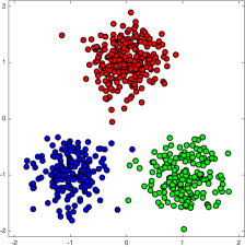
(a) Gaussian blobs

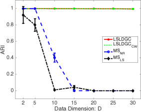
(b) $n=600$

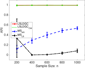
(c) $D=10$

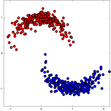
(d) Two curves

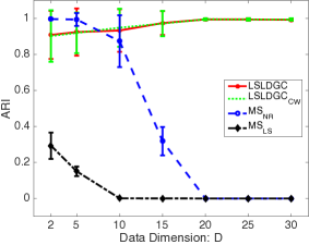
(e) $n=600$

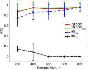
(f) $D=10$

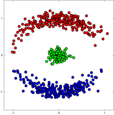
(g) Two curves & a Gaussian blob

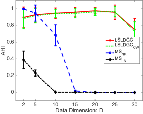
(h) $n=600$

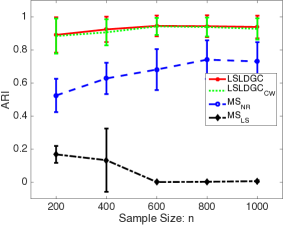
(i) $D=10$

Figure 6: Clustering performance on artificial data. Each point and error bar denote the average and standard deviation of ARI over $50$ runs, respectively.

5.1.2 Benchmark Datasets

Table 1: The average and standard deviation of ARI values over $50$ runs. A larger value means a better result. Numbers in the parentheses are standard deviations. The best and comparable methods judged by the unpaired t-test at the significance level $1\%$ are described in boldface.

Banknote $(D,n,c)=(4,100,2)$
LSLDGC	LSLDGC${}_{\text{CW}}$	MS${}_{\text{LS}}$	MS${}_{\text{NR}}$	SC	KM
0.165(0.059)	0.169(0.055)	0.036(0.014)	0.167(0.147)	0.054(0.064)	0.039(0.051)

Accelerometry $(D,n,c)=(5,300,3)$
LSLDGC	LSLDGC${}_{\text{CW}}$	MS${}_{\text{LS}}$	MS${}_{\text{NR}}$	SC	KM
0.628(0.058)	0.624(0.065)	0.029(0.007)	0.500(0.041)	0.226(0.271)	0.499(0.023)

Olive oil $(D,n,c)=(8,200,9)$
LSLDGC	LSLDGC${}_{\text{CW}}$	MS${}_{\text{LS}}$	MS${}_{\text{NR}}$	SC	KM
0.717(0.081)	0.728(0.062)	0.020(0.019)	0.756(0.078)	0.552(0.060)	0.618(0.063)

Vowel $(D,n,c)=(10,110,11)$
LSLDGC	LSLDGC${}_{\text{CW}}$	MS${}_{\text{LS}}$	MS${}_{\text{NR}}$	SC	KM
0.147(0.037)	0.139(0.032)	0.017(0.010)	0.133(0.026)	0.145(0.027)	0.180(0.027)

Sat-image $(D,n,c)=(36,120,6)$
LSLDGC	LSLDGC${}_{\text{CW}}$	MS${}_{\text{LS}}$	MS${}_{\text{NR}}$	SC	KM
0.427(0.072)	0.422(0.073)	0.000(0.000)	0.343(0.063)	0.418(0.056)	0.434(0.052)

Speech $(D,n,c)=(50,400,2)$
LSLDGC	LSLDGC${}_{\text{CW}}$	MS${}_{\text{LS}}$	MS${}_{\text{NR}}$	SC	KM
0.146(0.063)	0.147(0.054)	0.000(0.000)	0.000(0.000)	0.004(0.004)	0.002(0.004)

Next, we investigate the performance of LSLDGC over the following benchmark datasets:

• Banknote $(D=4,n=100,~{}\mathrm{and}~{}c=2)$ (Bache and Lichman, 2013): This dataset consists of four-dimensional features from $400$ by $400$ images for genuine and forged banknote-like specimens. The features were extracted by wavelet transformation. We randomly chose $50$ samples from each of the two classes.

• Accelerometry $(D=5,n=300,~{}\mathrm{and}~{}c=3)$: The ALKAN dataset contains $3$-axis (i.e., x-, y-, and z-axes) accelerometric data. During the data collection, subjects were instructed to perform walking, running, and standing up. After segmenting each data stream into windows, five orientation-invariant-features were computed from each window (Sugiyama et al., 2014). We randomly chose $100$ samples from each of the three classes.

• Olive oil $(D=8,n=200,~{}\mathrm{and}~{}c=9)$ (Forina et al., 1983). This dataset was obtained from the R software. The dataset includes eight chemical measurements on different specimen of olive oil produced in nine regions in Italy. We randomly chose $200$ samples.

• Vowel $(D=10,n=110,~{}\mathrm{and}~{}c=11)$ (Turney, 1993; Bache and Lichman, 2013): This consists utterance data for eleven vowels of British English. Each utterance is expressed by a ten-dimensional vector. We randomly chose $10$ samples from each of the eleven classes.

• Sat-image $(D=36,n=120,~{}\mathrm{and}~{}c=6)$ (Bache and Lichman, 2013): The dataset contains the multi-spectral values of pixels in $3\times 3$ neighborhoods in a satellite image with six classes. We randomly chose $20$ samples from each of the six classes.

• Speech $(D=50,n=400,~{}\mathrm{and}~{}c=2)$. An in-house speech dataset (Sugiyama et al., 2014), which contains short utterance samples recorded from $2$ male subjects speaking in French with sampling rate $44.1$kHz. 50-dimensional line spectral frequencies vectors (Kain and Macon, 1998) were computed from each utterance sample. We randomly chose $200$ samples from each of the two classes.

As preprocessing, each data sample was standardized by the sample mean and standard deviation in coordinate-wise manner. For comparison, we applied k-means clustering (KM) (MacQueen, 1967) and spectral clustering (SC) (Ng et al., 2001; Shi and Malik, 2000) to the same datasets. Since KM and SC require to input the number of clusters, we set it at the correct number.

As seen in the illustration on artificial data, when the dimensionality of data is low, the performance of LSLDGC, LSLDGC${}_{\text{CW}}$ and MS${}_{\text{NR}}$ is comparable, but LSLDGC and LSLDGC${}_{\text{CW}}$ significantly work better than MS${}_{\text{NR}}$ to higher-dimensional datasets (sat-image and speech datasets). KM and SC have prior information about the number of clusters. Nonetheless, the performance of LSLDGC and LSLDGC${}_{\text{CW}}$ are often better than KM and SC.

From the results of both the artificial and benchmark datasets, we conclude that LSLDGC and LSLDGC${}_{\text{CW}}$ are advantageous to relatively high-dimensional data.

5.2 Illustration on Density Ridge Estimation

Next, we illustrate the performance of LSDRF, and compare LSDRF with SCMS both on artificial and standard benchmark datasets.

5.2.1 Artificial Data: LSDRF vs SCMS

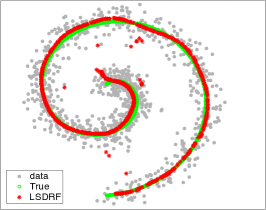
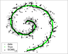
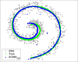
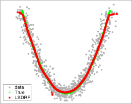
(a) LSDRF

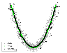
(b) SCMS${}_{\text{LS}}$

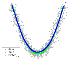
(c) SCMS${}_{\text{CR}}$

Figure 7: Comparison of the two estimated ridges by LSDRF, SCMS${}_{\text{LS}}$ and SCMS${}_{\text{CR}}$.

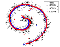
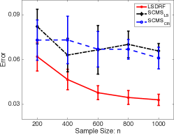
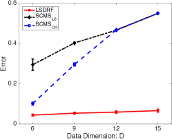
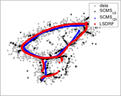
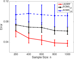
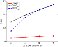
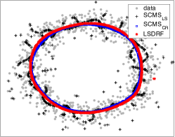
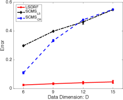
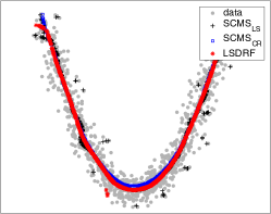
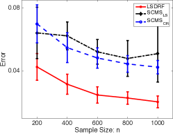
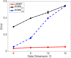
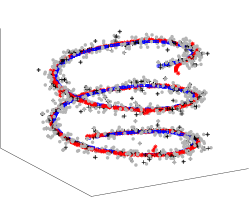
(a) Density ridge estimates

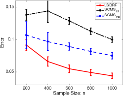
(b) Error against sample size

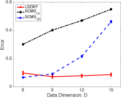
(c) Error against data dimension

Figure 8: Performance of ridge estimation on artificial data. Each point and error bar denote the average and standard deviation of ARI over $50$ runs, respectively. For (c), $n=1000$. Errors for ridge estimation are computed according to (37).

The performance of LSDRF is compared to SCMS with two different bandwidth selection methods:

• LSDRF: When estimating $g_{j}(\bm{x})$, we selected ten candidates of the width parameter in the Gaussian kernel and the regularization parameter from $10^{l}\times\sigma^{(j)}_{\text{med}}$ ($-0.3\leq l\leq 1$) and $10^{m}$ ($-4\leq m\leq 0$), respectively. When estimating $[\bm{H}(\bm{x})]_{ij}$, ten candidates of the width parameter in the Gaussian kernel were selected from $10^{l}\times\sqrt{\sigma^{(i)}_{\text{med}}\sigma^{(j)}_{\text{med}}}$ ($-0.3\leq l\leq 1$). For the regularization parameter, we used the same candidates as in $g_{j}(\bm{x})$.

• SCMS${}_{\text{LS}}$: The bandwidth parameter $h$ was cross-validated based on the standard integrated squared error. We selected ten candidates of $h$ from $10^{l}\times h_{\text{med}}$ ($-1.5\leq l\leq 0$) where $h_{\text{med}}$ is the median value of $|x_{i}^{(j)}-x_{k}^{(j)}|$ with respect to $i$, $j$ and $k$.

• SCMS${}_{\text{CR}}$: The bandwidth parameter $h$ was cross-validated based on the coverage risk proposed in Chen et al. (2015a). As suggested in Chen et al. (2015a), we selected ten candidates of $h$ from $10^{l}\times h_{\text{NR}}$ ($-1\leq l\leq 0$) where $h_{\text{NR}}$ is the bandwidth based on the normal reference rule (Silverman, 1986).

We investigate the performance of these methods on a variety of simulated datasets. The $i$-th observation of data was generated according to $x_{i}^{(j)}=f^{(j)}(t_{i})+n^{(j)}_{i}$, where $t_{i}$ was taken from some range at regular intervals, $f^{(j)}(\cdot)$ denotes some fixed function, and $n^{(j)}_{i}$ was the Gaussian noise with mean $0$ and standard deviation $0.15$. Higher-dimensional data were created by appending the Gaussian variables with mean $0$ and standard deviation $0.15$. The estimation error was measured by

$$\text{Error}=\frac{1}{n}\sum_{i=1}^{n}\min_{l}\|\widehat{\bm{y}}_{i}-\bm{f}(t_{l})\|,$$ (37)

where $\bm{f}(\cdot)=(f^{(1)}(\cdot),f^{(2)}(\cdot),\dots,f^{(D)}(\cdot))^{\top}$ and $\widehat{\bm{y}}_{i}$ denotes an estimate of the density ridge point from $\bm{x}_{i}$.

The estimated ridges are visualized in Fig.7. SCMS${}_{\text{LS}}$ provides a broken and non-smooth ridge estimate because the selected bandwidth by the least-squares cross-validation is small for density ridge estimation as in mode-seeking clustering. In contrast, the ridges estimated by LSDRF and SCMS${}_{\text{CR}}$ are smooth. However, SCMS${}_{\text{CR}}$ gives a biased estimate around highly curved region in the true ridge (e.g., the centers of the spiral and quadratic curve in Fig.7), while the bias in LSDDR seems smaller. This implies that LSDRF more accurately estimates density ridges. The accuracy of LSDRF is quantified on a variety of artificial datasets in Fig 8. LSDRF produces smaller errors particularly when the sample size is large (Fig 8(b)). In addition, as in mode-seeking clustering, the performance of LSDRF is even better when the dimensionality of data is higher (Fig. 8(c)). This implies that our direct approach is useful for high(er)-dimensional data.

5.2.2 Density Ridge Estimation on Real-World Datasets

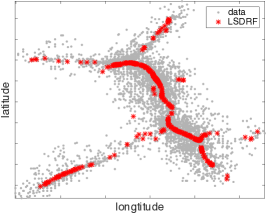
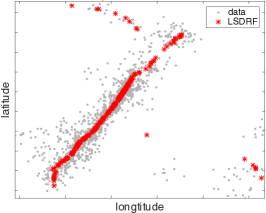
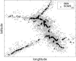
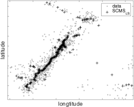
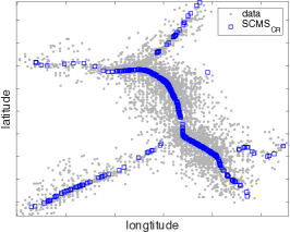
(a) Madrid 1

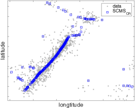
(b) Madrid 2

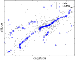
(c) Madrid 3

Figure 9: Density ridge estimation to three regions in the New Madrid earthquake dataset. The three regions (a,b,c) were extracted according to a range of latitude and longitude. The first, second and third rows correspond to results from LSDRF, SCMS${}_{\text{LS}}$ and SCMS${}_{\text{CR}}$, respectively.

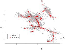
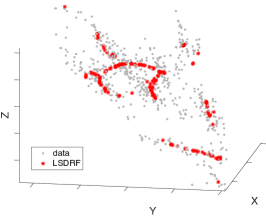
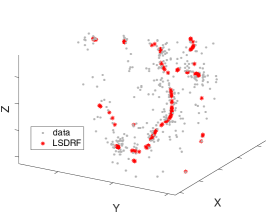
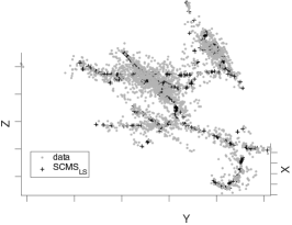
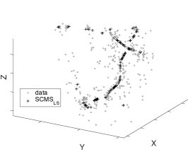
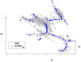
(a) Shapley 1

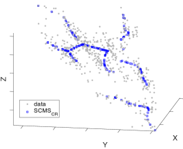
(b) Shapley 2

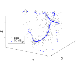
(c) Shapley 3

Figure 10: Density ridge estimation to three regions in the Shapley galaxy dataset. The three regions were extracted according to a range of recession velocity. The first, second and third rows correspond to results from LSDRF, SCMS${}_{\text{LS}}$ and SCMS${}_{\text{CR}}$, respectively.

Next, we apply LSDRF to real-world datasets. As in Pulkkinen (2015), we employed the following two datasets:

• New Madrid earthquake dataset: This seismological dataset was downloaded from the Center for Earthquake Research and Information. The dataset contains positional information for earthquakes around the New Madrid seismic zone from $1974$ to $2016$, providing $11,131$ samples. The three regions in Figs.9(a,b,c) were extracted according to (a) $(-90.2,-89.25)$, (b) $(-92.5,-92.15)$ and (c) $(-85.5,-83.5)$ degrees for the latitude range, respectively. For the longitude range, (a) $(36,36.8)$, (b) $(35.2,35.4)$ and (c) $(34.5,36.5)$ degrees were selected. The total numbers of the original data samples and reduced data samples in each region were (a) $(N,n)=(5902,500)$, (b) $(N,n)=(1548,300)$ and (c) $(N,n)=(594,200)$.

• Shapley galaxy dataset: This dataset was downloaded from the Center for Astrostatistics at Pennsylvania State University. The dataset contains information about the three-dimensional sky angles and recession velocity of $4,215$ galaxies. As done in Pulkkinen (2015), we transformed the data samples into the three-dimensional Cartesian coordinates based on the fact that the recession velocity is proportional to the radial distance (Drinkwater et al., 2004). The three regions in Figs 10(a,b,c) were extracted according to a velocity range: (a) $(6000,20000)$ km/s, (b) $(1500,6000)$ km/s and (c) $(6000,10500)$ km/s, respectively. The total numbers of the original data samples and reduced data samples in each region were (a) $(N,n)=(2849,500)$, (b) $(N,n)=(595,200)$ and (c) $(N,n)=(351,150)$.

In each dataset, we focused on three regions containing prominent features, and standardized data samples in each region by subtracting the mean value and dividing by standard deviation in a dimension-wise manner. Here, the standardized data samples are collectively denoted by $\widetilde{\mathcal{D}}=\{\widetilde{\bm{x}}_{i}\}_{i=1}^{N}$. Before applying density ridge estimation methods, we performed preprocessing to remove clutter noises: KDE was applied to the dataset of each region, and then the data samples $\widetilde{\bm{x}}_{i}$ in each region were removed when $\frac{\widehat{p}_{\text{KDE}}(\widetilde{\bm{x}}_{i})}{\max_{j}[\widehat{p}_{\text{KDE}}(\widetilde{\bm{x}}_{j})]}<10^{-3}$. After noise removal, we randomly chose $n$ data samples from each region, and applied the three density ridge estimation methods to the sub-sampled data. The sub-sampled data are collectively expressed by $\mathcal{D}=\{\bm{x}_{i}\}_{i=1}^{n}$. For performance comparison, we computed the logarithm of $\widehat{p}_{\text{KDE}}$ on the estimated density ridges, which is given by

$$\mathcal{L}=\frac{1}{n}\sum_{i=1}^{n}\log\widehat{p}_{\text{KDE}}(\widehat{\bm{y}}_{i}),$$

where the centers of the kernel function in $\widehat{p}_{\text{KDE}}$ were set at the original data samples $\widetilde{\bm{x}}_{i}$ in each region, and $\widehat{\bm{y}}_{i}$ denotes an estimated density ridge point from $\bm{x}_{i}$. If $\mathcal{L}$ is larger, the performance can be interpreted to be better because ridges are defined on relatively high density areas. Unlike the last illustration, for SCMS_LS, we employed the following adaptive-bandwidth Gaussian kernel:

$$\frac{1}{(2\pi h_{i}^{2})^{D/2}}\exp\left(-\frac{\|\bm{x}-\bm{x}_{i}\|^{2}}{2h_{i}^{2}}\right),$$

where $h_{i}$ denotes the bandwidth parameter. We restricted $h_{i}$ at the $m$-nearest neighbor Euclidean distance from $\bm{x}_{i}$ to $\bm{x}_{j}~{}(i\neq j)$, and performed cross-validation with respect to $m$ whose candidates were $128$, $64$, $32$, $16$, $8$ and $4$. For SCMS_LS, the ten candidates of the bandwidth parameter were selected from $10^{l}\times h_{\text{NR}}$ ($-0.3\leq l\leq 0$). For LSDRF, we employed all data samples $\{\bm{x}_{i}\}_{i=1}^{n}$ as the centers of the Gaussian kernel, and used the median value of $\text{CV}(t)$ in Section 2.4 instead of the mean value in cross-validation.

Ridges estimated by LSDRF are smooth and seem to qualitatively well-match the ridges in the underlying data, and SCMS${}_{\text{CR}}$ and SCMS${}_{\text{LS}}$ also perform fairly good (Figs.9 and 10). Table 2 is quantitative comparison by $\mathcal{L}$, showing that LSDRF compares favorably with both SCMS${}_{\text{CR}}$ and SCMS${}_{\text{LS}}$.

Table 2: The average and standard deviation of the performance measure $\mathcal{L}$ over $50$ runs. Madrid 1, 2 and 3 (or Shapley 1, 2 and 3) correspond to the three regions in Fig.9 (or Fig.10). A larger value means a better result. Numbers in the parentheses are standard deviations. The best and comparable methods judged by the unpaired t-test at the significance level $1\%$ are described in boldface.

New Madrid earthquake
	LSDRF	SCMS${}_{\text{LS}}$	SCMS${}_{\text{CR}}$
Madrid 1	-0.511(0.101)	-0.610(0.072)	-0.571(0.075)
Madrid 2	0.001(0.175)	0.029(0.065)	-0.076(0.075)
Madrid 3	-1.173(0.132)	-1.238(0.086)	-1.238(0.098)

Shapley galaxy
	LSDRF	SCMS${}_{\text{LS}}$	SCMS${}_{\text{CR}}$
Shapley 1	0.188(0.093)	0.094(0.073)	0.063(0.121)
Shapley 2	-1.120(0.145)	-1.220(0.097)	-1.462(0.223)
Shapley 3	-1.295(0.114)	-1.544(0.076)	-1.581(0.091)

6 Conclusion

In this paper, we proposed a novel estimator of the ratios of the density derivatives to the density. In stark contrast with the approaches in mean shift clustering and subspace constrained mean shift, our approach is to directly estimate the density-derivative-ratios without going through density estimation and computing the ratios. The proposed estimator was theoretically investigated, and the convergence rate was established. We applied the proposed estimator to mode-seeking clustering and density ridge estimation, and developed practical methods. Moreover, theoretical analysis were also performed to these methods , and the convergence rates to the mode and ridge of the true density were established. Our experimental illustration demonstrated that the proposed methods for mode-seeking clustering and density ridge estimation outperformed existing methods particularly for high(er)-dimensional data.

This paper focused only on mode-seeking clustering and density ridge estimation. The proposed estimator can be useful or extended for other problems. For instance, making use of the global mode (the global maximum) of a conditional density enables us to develop a regression method robust against outliers (Yao et al., 2012). Non-parametric estimation of the mode is also needed in functional data analysis (Gasser et al., 1998). In future, we explore novel applications of the proposed estimator.

Acknowledgements

The authors are grateful to Dr. Matthew James Holland for his helpful comments on an earlier version of this paper. Takafumi Kanamori was supported by KAKENHI 16K00044, 15H03636, and 15H01678. Aapo Hyvärinen was supported by the Academy of Finland. Gang Niu was supported by CREST JPMJCR1403. Masashi Sugiyama was supported by the International Research Center for Neurointelligence (WPI-IRCN) at The University of Tokyo Institutes for Advanced Study.

Appendix A Proof of Theorem 1

Proof  We first derive the following two lemmas by modifying the proof techniques in Sriperumbudur et al. (2013):

Lemma 15

With $\epsilon=1$ in Assumption (D), the following statements hold:

1. For $J_{\bm{j}}$ with the regularizer,

   $$J_{\bm{j}}^{\lambda}(r_{\bm{j}}):=J_{\bm{j}}(r_{\bm{j}})+\lambda_{\bm{j}}\|r_{\bm{j}}\|^{2}_{\mathcal{H}},$$

   the minimizer of $J_{\bm{j}}^{\lambda}$ is given by

   $$r_{\bm{j}}^{\lambda}:=\mathop{\rm argmin}\limits_{r_{\bm{j}}\in\mathcal{H}}J_{\bm{j}}^{\lambda}(r_{\bm{j}})=(C+\lambda_{\bm{j}}I)^{-1}\xi_{\bm{j}}=(C+\lambda_{\bm{j}}I)^{-1}Cr_{\bm{j}}^{*},$$

   where $C=\int_{\mathcal{X}}k(\cdot,\bm{x})\otimes k(\cdot,\bm{x})p(\bm{x})\mathrm{d}\bm{x}$, $\otimes$ is the tensor product, and

   $$\xi_{\bm{j}}:=(-1)^{|\bm{j}|}\int_{\mathcal{X}}\partial_{\bm{j}}k(\cdot,\bm{x})p(\bm{x})\mathrm{d}\bm{x}.$$

2. $\widehat{J}_{\bm{j}}(r_{\bm{j}})$ can be equivalently expressed as

   $$\widehat{J}_{\bm{j}}(r_{\bm{j}})=\langle r_{\bm{j}}-r_{\bm{j}}^{*},\widehat{C}(r_{\bm{j}}-r_{\bm{j}}^{*})\rangle_{\mathcal{H}},$$

   where

   $$\widehat{C}:=\frac{1}{n}\sum_{i=1}^{n}k(\cdot,\bm{x}_{i})\otimes k(\cdot,\bm{x}_{i})\quad\text{and}\quad\widehat{\xi}_{\bm{j}}:=\frac{(-1)^{|\bm{j}|}}{n}\sum_{i=1}^{n}\partial_{\bm{j}}k(\cdot,\bm{x}_{i}).$$

   Then, $\widehat{r}_{\bm{j}}$ is given by

   $$\widehat{r}_{\bm{j}}=\mathop{\rm argmin}\limits_{r_{\bm{j}}\in\mathcal{H}}\left[\widehat{J}_{\bm{j}}(r_{\bm{j}})+\lambda_{\bm{j}}\|r_{\bm{j}}\|^{2}_{\mathcal{H}}\right]=(\widehat{C}+\lambda_{\bm{j}}I)^{-1}\widehat{\xi}_{\bm{j}}.$$

Lemma 16

With $\epsilon=2$ in Assumption (D),

$$\|\widehat{\xi}_{\bm{j}}-\widehat{C}r_{\bm{j}}^{*}\|_{\mathcal{H}}=O_{\mathrm{P}}\left(n^{-1/2}\right).$$ (38)

The proofs of these lemmas can be seen in Appendices A.1 and A.2, respectively.

Next, we make use of the proof of Theorem 5 in Sriperumbudur et al. (2013) to prove Theorem 1. From Lemma 15,

$$\widehat{r}_{\bm{j}}-r_{\bm{j}}^{\lambda} =(\widehat{C}+\lambda_{\bm{j}}I)^{-1}\widehat{\xi}_{\bm{j}}-r_{\bm{j}}^{\lambda}$$

$$=(\widehat{C}+\lambda_{\bm{j}}I)^{-1}\left\{\widehat{\xi}_{\bm{j}}-\widehat{C}r_{\bm{j}}^{\lambda}-\lambda_{\bm{j}}r_{\bm{j}}^{\lambda}\right\}$$

$$=(\widehat{C}+\lambda_{\bm{j}}I)^{-1}(\widehat{\xi}_{\bm{j}}-\widehat{C}r_{\bm{j}}^{*})+(\widehat{C}+\lambda_{\bm{j}}I)^{-1}(C-\widehat{C})(r_{\bm{j}}^{\lambda}-r_{\bm{j}}^{*}),$$

where we used $\lambda_{\bm{j}}r_{\bm{j}}^{\lambda}=C(r_{\bm{j}}^{*}-r_{\bm{j}}^{\lambda})$ from Lemma 15(i). Therefore,

$$\|\widehat{r}_{\bm{j}}-r_{\bm{j}}^{*}\|_{\mathcal{H}} \leq\|\widehat{r}_{\bm{j}}-r_{\bm{j}}^{\lambda}\|_{\mathcal{H}}+\|r_{\bm{j}}^{\lambda}-r^{*}_{\bm{j}}\|_{\mathcal{H}}.$$

$$\leq\|(\widehat{C}+\lambda_{\bm{j}}I)^{-1}\|(\|\widehat{\xi}_{\bm{j}}-\widehat{C}r_{\bm{j}}^{*}\|_{\mathcal{H}}+\|C-\widehat{C}\|\mathcal{A}_{0}(\lambda_{\bm{j}}))+\mathcal{A}_{0}(\lambda_{\bm{j}}),$$

where $\mathcal{A}_{0}(\lambda_{\bm{j}})=\|r_{\bm{j}}^{\lambda}-r_{\bm{j}}^{*}\|_{\mathcal{H}}$. It can be shown that $\|(\widehat{C}+\lambda_{\bm{j}}I)^{-1}\|\leq 1/\lambda_{\bm{j}}$ for sufficiently small $\lambda_{\bm{j}}$. Thus, Lemma 16 shows that the first term can be bounded by $O_{\mathrm{P}}\left(\frac{1}{\lambda_{\bm{j}}\sqrt{n}}\right)$. In addition, with the proof techniques in Fukumizu et al. (2007, Lemma 5), $\|C-\widehat{C}\|\leq\|C-\widehat{C}\|_{\text{HS}}=O_{\mathrm{P}}(n^{-1/2})$ with $\epsilon=2$ where $\|\cdot\|_{\mathrm{HS}}$ denotes the Hilbert-Schmidt norm. Thus, the second term is of the order $O_{\mathrm{P}}\left(\frac{\mathcal{A}_{0}(\lambda_{\bm{j}})}{\sqrt{n}\lambda_{\bm{j}}}\right)$. From these results,

$$\|\widehat{r}_{\bm{j}}-r_{\bm{j}}^{*}\|_{\mathcal{H}} \leq O_{\mathrm{P}}\left(\frac{1}{\lambda_{\bm{j}}\sqrt{n}}\right)+O_{\mathrm{P}}\left(\frac{\mathcal{A}_{0}(\lambda_{\bm{j}})}{\sqrt{n}\lambda_{\bm{j}}}\right)+\mathcal{A}_{0}(\lambda_{\bm{j}}).$$ (39)

Propostion A.2 in Sriperumbudur et al. (2013) states that if $r_{\bm{j}}^{*}\in\mathcal{R}(C^{\gamma})$ and $C$ is a bounded and self-adjoint compact operator on a separable $\mathcal{H}$, the following inequality holds:

$$\mathcal{A}_{0}(\lambda_{\bm{j}})\leq\max(1,\|C\|^{\gamma-1})\lambda_{\bm{j}}^{\min(1,\gamma)}\|C^{-\gamma}r_{\bm{j}}^{*}\|_{\mathcal{H}}.$$ (40)

It can be easily verified that $C$ is a self-adjoint operator. Assumption (D) with $\epsilon=2$ ensures that $C$ is a Hilbert-Schmidt operator and therefore compact because it is bounded in terms of the Hilbert-Schmidt norm. Thus, applying (40) to (39) completes the proof when choosing $\lambda_{\bm{j}}=O\left(n^{-\max\left\{\frac{1}{4},\frac{1}{2(\gamma+1)}\right\}}\right)$ as $n\rightarrow\infty$.  

A.1 Proof of Lemma 15

Proof  (i) From the definition of $J_{\bm{j}}$,

$$J_{\bm{j}}(r_{\bm{j}}) =\int_{\mathcal{X}}\left\{r_{\bm{j}}(\bm{x})-r_{\bm{j}}^{*}(\bm{x})\right\}^{2}p(\bm{x})\mathrm{d}\bm{x}$$

$$=\int_{\mathcal{X}}\langle r_{\bm{j}}-r_{\bm{j}}^{*},k(\cdot,\bm{x})\rangle_{\mathcal{H}}^{2}p(\bm{x})\mathrm{d}\bm{x}$$

$$=\int_{\mathcal{X}}\langle r_{\bm{j}}-r_{\bm{j}}^{*},(k(\cdot,\bm{x})\otimes k(\cdot,\bm{x}))(r_{\bm{j}}-r_{\bm{j}}^{*})\rangle_{\mathcal{H}}p(\bm{x})\mathrm{d}\bm{x}$$

$$=\int_{\mathcal{X}}\langle r_{\bm{j}}-r_{\bm{j}}^{*},C_{\mathrm{x}}(r_{\bm{j}}-r_{\bm{j}}^{*})\rangle_{\mathcal{H}}p(\bm{x})\mathrm{d}\bm{x}$$

$$=\langle r_{\bm{j}}-r_{\bm{j}}^{*},C(r_{\bm{j}}-r_{\bm{j}}^{*})\rangle_{\mathcal{H}},$$

where $C_{\mathrm{x}}:=k(\cdot,\bm{x})\otimes k(\cdot,\bm{x})$. Expanding the right-hand side above transforms $J_{\bm{j}}^{\lambda}$ as

$$J_{\bm{j}}^{\lambda}(r_{\bm{j}}) =\langle r_{\bm{j}},Cr_{\bm{j}}\rangle_{\mathcal{H}}-2\langle r_{\bm{j}},Cr_{\bm{j}}^{*}\rangle_{\mathcal{H}}+\langle r_{\bm{j}}^{*},Cr_{\bm{j}}^{*}\rangle_{\mathcal{H}}+\lambda_{\bm{j}}\langle r_{\bm{j}},r_{\bm{j}}\rangle_{\mathcal{H}}$$

$$=\langle r_{\bm{j}},(C+\lambda_{\bm{j}}I)r_{\bm{j}}\rangle_{\mathcal{H}}-2\langle r_{\bm{j}},Cr_{\bm{j}}^{*}\rangle_{\mathcal{H}}+\langle r_{\bm{j}}^{*},Cr_{\bm{j}}^{*}\rangle_{\mathcal{H}}.$$ (41)

For the second term in (41), we compute

$$\langle r_{\bm{j}},Cr_{\bm{j}}^{*}\rangle_{\mathcal{H}} =\langle r_{\bm{j}},\int_{\mathcal{X}}k(\cdot,\bm{x})r_{\bm{j}}^{*}(\bm{x})p(\bm{x})\mathrm{d}\bm{x}\rangle_{\mathcal{H}}$$

$$=\langle r_{\bm{j}},\int_{\mathcal{X}}k(\cdot,\bm{x})\partial_{\bm{j}}p(\bm{x})\mathrm{d}\bm{x}\rangle_{\mathcal{H}}$$

$$=\langle r_{\bm{j}},(-1)^{|\bm{j}|}\int_{\mathcal{X}}\partial_{\bm{j}}k(\cdot,\bm{x})p(\bm{x})\mathrm{d}\bm{x}\rangle_{\mathcal{H}}$$

$$=\langle r_{\bm{j}},\xi_{\bm{j}}\rangle_{\mathcal{H}},$$ (42)

where we applied Assumption (C), and

$$\xi_{\bm{j}}=(-1)^{|\bm{j}|}\int_{\mathcal{X}}\partial_{\bm{j}}k(\cdot,\bm{x})p(\bm{x})\mathrm{d}\bm{x}.$$

Comparing the left-hand side with the right-hand side at the last line in (42) gives

$$Cr_{\bm{j}}^{*}=\xi_{\bm{j}}.$$ (43)

Eq.(43) is valid because (42) holds for arbitrary $r_{\bm{j}}\in\mathcal{H}$.

Simple calculation after substituting (42) into (41) provides

$$J_{\bm{j}}^{\lambda}(r_{\bm{j}}) =\|(C+\lambda_{\bm{j}}I)^{1/2}r_{\bm{j}}-(C+\lambda_{\bm{j}}I)^{-1/2}\xi_{\bm{j}}\|_{\mathcal{H}}^{2}-\langle\xi_{\bm{j}},(C+\lambda_{\bm{j}}I)^{-1}\xi_{\bm{j}}\rangle_{\mathcal{H}}+\langle r_{\bm{j}}^{*},Cr_{\bm{j}}^{*}\rangle_{\mathcal{H}},$$

Since the second and third terms in the right-hand side above do not include $r_{\bm{j}}$, the minimizer of $J_{\bm{j}}^{\lambda}(r_{\bm{j}})$ is given by $r_{\bm{j}}^{\lambda}=(C+\lambda_{\bm{j}}I)^{-1}\xi_{\bm{j}}=(C+\lambda_{\bm{j}}I)^{-1}Cr_{\bm{j}}^{*}$ where (43) was applied.

(ii) It follows from (i) by substituting $C$ and $\xi_{\bm{j}}$ with $\widehat{C}$ and $\widehat{\xi}_{\bm{j}}$, respectively.  

A.2 Proof of Lemma 16

Proof  We first compute the expectation of $\|\widehat{\xi}_{\bm{j}}-\widehat{C}r_{\bm{j}}^{*}\|_{\mathcal{H}}^{2}$ as

$$E\|\widehat{\xi}_{\bm{j}}-\widehat{C}r_{\bm{j}}^{*}\|_{\mathcal{H}}^{2}=\frac{n-1}{n}\|\xi_{\bm{j}}-Cr_{\bm{j}}^{*}\|^{2}_{\mathcal{H}}+\frac{1}{n}\int_{\mathcal{X}}\|(-1)^{|\bm{j}|}\partial_{\bm{j}}k(\cdot,\bm{x})+C_{\mathrm{x}}r_{\bm{j}}^{*}\|^{2}_{\mathcal{H}}p(\bm{x})\mathrm{d}\bm{x},$$ (44)

where $C_{\mathrm{x}}=k(\cdot,\bm{x})\otimes k(\cdot,\bm{x})$. Eq.(43) indicates that the first term in the right-hand side of (44) vanishes, i.e., $\|\xi_{\bm{j}}-Cr_{\bm{j}}^{*}\|_{\mathcal{H}}=0$. From

$$\|(-1)^{|\bm{j}|}\partial_{\bm{j}}k(\cdot,\bm{x})+C_{\mathrm{x}}r_{\bm{j}}^{*}\|^{2}_{\mathcal{H}}\leq 2\|\partial_{\bm{j}}k(\cdot,\bm{x})\|^{2}_{\mathcal{H}}+2\|C_{\mathrm{x}}\|^{2}_{\text{HS}}\|r_{\bm{j}}^{*}\|^{2}_{\mathcal{H}},$$

Assumption (D) with $\epsilon=2$ ensures that the second term in the right-hand side of (44) is finite. Thus, applying the Chebyshev’s inequality proves the lemma because $E(\widehat{\xi}_{\bm{j}}-\widehat{C}r_{\bm{j}}^{*})=\xi_{\bm{j}}-Cr_{\bm{j}}^{*}=0$ from (43).  

Appendix B Connection to the Minimax Theory

This appendix provides details for the connections to the minimax theory discussed in the remark after Theorem 1. First, we introduce the following results:

• By the minimax theory (Tsybakov, 2009), Eq.(10) in Sriperumbudur et al. (2017) shows the minimax rate: For any $\alpha>\delta\geq 0$,

  $$\inf_{\widehat{r}_{\bm{j},n}}\sup_{r_{\bm{j}}^{*}\in H^{\alpha}_{2}}\|\widehat{r}_{\bm{j},n}-r_{\bm{j}}^{*}\|_{H^{\delta}_{2}}\asymp n^{-\frac{\alpha-\delta}{2(\alpha-\delta)+D}}.$$ (45)

• The following proposition provides necessary conditions for $r_{\bm{j}}^{*}\in R(C)$:

  Proposition 17

  Suppose that $\psi,\phi\in C(\mathbb{R}^{D})\cap L^{1}(\mathbb{R}^{D})$ are real-valued, shift-invariant and positive definite kernel functions. Let $\mathcal{H}$ and $\mathcal{G}$ be RKHSs associated with $\psi(\bm{x}-\bm{y})$ and $\phi(\bm{x}-\bm{y})$, respectively. For $2\leq r\leq\infty$, assume that the followings hold,

  $$p\in L^{\frac{r}{r-1}}(\mathbb{R}^{D}),\quad\left\|\frac{\phi^{\wedge}}{\psi^{\wedge}}\right\|_{\infty}<\infty\quad\text{and}\quad\left\|\frac{\psi^{\wedge 2}}{\phi^{\wedge}}\right\|_{\frac{r}{r-2}}<\infty.$$

  Then, $r_{\bm{j}}^{*}\in R(C)$ implies that $r_{\bm{j}}^{*}\in\mathcal{G}\subset\mathcal{H}$, where $k(\bm{x},\bm{y})=\psi(\bm{x}-\bm{y})$ in the operator $C$.

  The proof of Proposition 17 is deferred to Section B.1. The conditions are necessary ones for $r_{\bm{j}}^{*}\in R(C^{\beta})$ with $\beta>1$ as well because $R(C^{\beta_{1}})\subset R(C^{\beta_{2}})$ for $0<\beta_{1}<\beta_{2}<\infty$ (Sriperumbudur et al., 2017, Section 4.2 and Appendix B.3).

Recall that when the Matérn kernel, $k(\bm{x},\bm{y})=\psi(\bm{x}-\bm{y})=\frac{2^{1-s}}{\Gamma(s)}\|\bm{x}-\bm{y}\|^{s-D/2}\mathfrak{K}_{D/2-s}(\|\bm{x}-\bm{y}\|)$, is employed, the corresponding RKHS $\mathcal{H}$ is the Sobolev space $H^{s}_{2}$ with $s>D/2$ (Wendland, 2004, Chapter 10):

$$\mathcal{H}=H^{s}_{2}:=\left\{f\in L^{2}(\mathbb{R}^{D})\cap C(\mathbb{R}^{D}):\int(1+\|\bm{\omega}\|^{2})^{s}|f^{\wedge}(\bm{\omega})|^{2}\mathrm{d}\bm{\omega}<\infty\right\}.$$

Theorem 6.13 in Wendland (2004) gives the Fourier transform of $\psi$ as

$$\psi^{\wedge}(\bm{\omega})=(1+\|\bm{\omega}\|^{2})^{-s}.$$

When $p\in L^{1}(\mathbb{R}^{D})$, applying Proposition 17 ensures that $r_{\bm{j}}^{*}\in R(C)$ implies $r_{\bm{j}}^{*}\in H^{s^{\prime}}_{2}\subset H^{s}_{2}$ with $\frac{D}{2}<s\leq s^{\prime}<2s+\frac{1}{2}-\frac{D}{2}$. Thus, $r_{\bm{j}}^{*}\in H^{2s+\frac{1}{2}-\frac{D}{2}-\epsilon}_{2}$ for arbitrarily small $\epsilon>0$. Then, if we chose $\mathcal{H}=H^{D-\frac{1}{2}+\epsilon}_{2}$, the rate $n^{-\frac{1}{4}}$ in Theorem 1 is minimax optimal (Set $\alpha=2s+\frac{1}{2}-\frac{D}{2}-\epsilon$ and $\delta=s$ in (45), equate the exponent in the right-hand side of (45) with $-\frac{1}{4}$, and solve it with respect to $s$). Similar discussion is possible when $p\in L^{2}(\mathbb{R}^{D})$: The rate is minimax optimal under the choice of $\mathcal{H}=H^{\frac{D}{2}+\epsilon}_{2}$.

B.1 Proof of Proposition 17

Here, we modify the proof of Proposition 8 in Sriperumbudur et al. (2017).

Proof  To characterize RKHSs induced by shift-invariant kernels, we employ the following lemma:

Lemma 18 (Theorem 10.12 in Wendland (2004))

Let $\psi(\bm{x}-\bm{y})$ be a real-valued, symmetric and positive definite kernel. When $\psi\in C(\mathbb{R}^{D})\cap L^{1}(\mathbb{R}^{D})$, it induces the following Hilbert space,

$$\mathcal{H}:=\left\{f\in C(\mathbb{R}^{D})\cap L^{2}(\mathbb{R}^{D}):\frac{f^{\wedge}}{\sqrt{\psi^{\wedge}}}\in L^{2}(\mathbb{R}^{D})\right\},$$

with the reproducing kernel $\psi(\bm{x}-\bm{y})$ and inner product,

$$\langle f,g\rangle_{\mathcal{H}}:=\frac{1}{(2\pi)^{D/2}}\int\frac{f^{\wedge}(\bm{\omega})\overline{g^{\wedge}(\bm{\omega})}}{\psi^{\wedge}(\bm{\omega})}\mathrm{d}\bm{\omega}.$$

$\overline{g^{\wedge}(\bm{\omega})}$ above denotes the complex conjugate of $g^{\wedge}(\bm{\omega})$. In particular, every $f$ in $\mathcal{H}$ can be recovered from its Fourier transform $f^{\wedge}\in L^{1}(\mathbb{R}^{D})\cap L^{2}(\mathbb{R}^{D})$ as

$$f(\bm{x})=\frac{1}{(2\pi)^{D/2}}\int f^{\wedge}(\bm{\omega})e^{i\bm{x}^{\top}\bm{\omega}}\mathrm{d}\bm{\omega}.$$ (46)

Let us express an RKHS $\mathcal{G}$ induced by another real-valued, symmetric and positive definite kernel $\phi(\bm{x}-\bm{y})$. We first show that $\mathcal{G}\subset\mathcal{H}$ if $\left\|\frac{\phi^{\wedge}(\bm{\omega})}{\psi^{\wedge}(\bm{\omega})}\right\|_{\infty}<\infty$. From Lemma 18, for $g\in\mathcal{G}$, the norm in $\mathcal{H}$ is computed as

$$\|g\|_{\mathcal{H}}^{2}=\frac{1}{(2\pi)^{D/2}}\int\frac{|g^{\wedge}(\bm{\omega})|^{2}}{\psi^{\wedge}(\bm{\omega})}\mathrm{d}\bm{\omega}=\frac{1}{(2\pi)^{D/2}}\int\frac{|g^{\wedge}(\bm{\omega})|^{2}\phi^{\wedge}(\bm{\omega})}{\phi^{\wedge}(\bm{\omega})\psi^{\wedge}(\bm{\omega})}\mathrm{d}\bm{\omega}\leq\|g\|_{\mathcal{G}}^{2}\left\|\frac{\phi^{\wedge}(\bm{\omega})}{\psi^{\wedge}(\bm{\omega})}\right\|_{\infty}<\infty.$$

Thus, $g\in\mathcal{H}$, which indicates that $\mathcal{G}\subset\mathcal{H}$.

Next, we show that $r_{\bm{j}}^{*}\in R(C)$ indicates $r_{\bm{j}}^{*}\in\mathcal{G}$. Since $r_{\bm{j}}^{*}\in R(C)$, there exists $f\in\mathcal{H}$ such that $r_{\bm{j}}^{*}=Cf$, i.e.,

$$r_{\bm{j}}^{*}(\bm{y}) =\int k(\bm{x},\bm{y})f(\bm{x})p(\bm{x})\mathrm{d}\bm{x}$$

$$=\int\psi(\bm{x}-\bm{y})f(\bm{x})p(\bm{x})\mathrm{d}\bm{x}$$

$$=\int\left[\frac{1}{(2\pi)^{D/2}}\int\psi^{\wedge}(\bm{\omega})e^{i(\bm{x}-\bm{y})^{\top}\bm{\omega}}\mathrm{d}\bm{\omega}\right]f(\bm{x})p(\bm{x})\mathrm{d}\bm{x}$$

$$=\int\left[\frac{1}{(2\pi)^{D/2}}\int f(\bm{x})p(\bm{x})e^{i\bm{x}^{\top}\bm{\omega}}\mathrm{d}\bm{x}\right]\psi^{\wedge}(\bm{\omega})e^{-i\bm{y}^{\top}\bm{\omega}}\mathrm{d}\bm{\omega}$$

$$=\int(f^{\wedge}*p^{\wedge})(-\bm{\omega})\psi^{\wedge}(\bm{\omega})e^{-i\bm{y}^{\top}\bm{\omega}}\mathrm{d}\bm{\omega},$$ (47)

where we applied (46) to $\psi(\bm{x}-\bm{y})$ on the third line and Fubini’s theorem on the fourth line, and $*$ denotes the convolution such that

$$(f*p)(\bm{x}):=\int f(\bm{y})p(\bm{x}-\bm{y})\mathrm{d}\bm{y}.$$

Eq.(47) indicates that the Fourier transform of $r_{\bm{j}}^{*}$ is given by

$$r_{\bm{j}}^{*\wedge}(\bm{\omega})=(f^{\wedge}*p^{\wedge})(-\bm{\omega})\psi^{\wedge}(\bm{\omega}).$$

Computing the norm of $r^{*}_{\bm{j}}$ in $\mathcal{G}$ yields

$$\|r^{*}_{\bm{j}}\|_{\mathcal{G}}^{2}=\int|(f^{\wedge}*p^{\wedge})(-\bm{\omega})|^{2}\frac{\psi^{\wedge}(\bm{\omega})^{2}}{\phi^{\wedge}(\bm{\omega})}\mathrm{d}\bm{\omega} \leq\|(f^{\wedge}*p^{\wedge})^{2}\|_{r/2}\left\|\frac{\psi^{\wedge 2}}{\phi^{\wedge}}\right\|_{\frac{r}{r-2}}=\|f^{\wedge}*p^{\wedge}\|_{r}^{2}\left\|\frac{\psi^{\wedge 2}}{\phi^{\wedge}}\right\|_{\frac{r}{r-2}},$$

where Hölder inequality was applied with $2\leq r\leq\infty$. Then, Young’s convolution and Hausdorff-Young inequalities (Beckner, 1975) yield

$$\|f^{\wedge}*p^{\wedge}\|_{r}\leq\|f^{\wedge}\|_{1}\cdot\|p^{\wedge}\|_{r}\leq\|f^{\wedge}\|_{1}\cdot\|p\|_{\frac{r}{r-1}}<\infty$$

Thus, by Lemma 18, $r_{\bm{j}}^{*}\in R(C)$ indicates $r_{\bm{j}}^{*}\in\mathcal{G}$.  

Appendix C Proof of Theorem 3

Proof  Suppose that $\widehat{\alpha}_{j}^{(i)}=0$ and $\widetilde{\beta}_{j}^{(i)}\left(=-\widehat{\beta}_{j}^{(i)}\right)\geq 0$ for all $i$ and $j$. Computing the integral in (18) shows that

$$\widehat{D}_{\widehat{\bm{g}}}[\bm{x}|\bm{y}] =\sum_{j=1}^{D}\int_{y^{(j)}}^{x^{(j)}}\widehat{g}_{j}(x^{(1)},\dots,x^{(j-1)},z^{(j)},y^{(j+1)},\dots,y^{(D)})\mathrm{d}z^{(j)}$$

$$=\sum_{j=1}^{D}\sum_{i=1}^{n}\widetilde{\beta}^{(i)}_{j}\left[\phi\left(\frac{\|\bm{z}_{x}^{j}-\bm{x}_{i}\|^{2}}{2\sigma_{j}^{2}}\right)-\phi\left(\frac{\|\bm{z}_{y}^{j}-\bm{x}_{i}\|^{2}}{2\sigma_{j}^{2}}\right)\right],$$ (48)

where we used the relation $\partial_{j}^{\prime}\phi\left(\|\bm{x}-\bm{x}^{\prime}\|^{2}\right)=-\partial_{j}\phi\left(\|\bm{x}-\bm{x}^{\prime}\|^{2}\right)$, and

$$\bm{z}_{y}^{j} =(x^{(1)},\dots,x^{(j-1)},y^{(j)},y^{(j+1)},\dots,y^{(D)})^{\top}$$

$$\bm{z}_{x}^{j} =(x^{(1)},\dots,x^{(j-1)},x^{(j)},y^{(j+1)},\dots,y^{(D)})^{\top}.$$ (49)

Note that the $j$-th elements in $\bm{z}_{y}^{j}$ and $\bm{z}_{x}^{j}$ only differ. To ensure that the right-hand side in (48) is non-negative, we need to show that for all $j$,

$$\sum_{i=1}^{n}\widetilde{\beta}^{(i)}_{j}\left[\phi\left(\frac{\|\bm{z}_{x}^{j}-\bm{x}_{i}\|^{2}}{2\sigma_{j}^{2}}\right)-\phi\left(\frac{\|\bm{z}_{y}^{j}-\bm{x}_{i}\|^{2}}{2\sigma_{j}^{2}}\right)\right]\geq 0.$$ (50)

To obtain a lower bound of the left-hand side in (50), we use the following inequality, which comes from the convexity of $\phi$:

$$\phi\left(\frac{\|\bm{z}_{x}^{j}-\bm{x}_{i}\|^{2}}{2\sigma_{j}^{2}}\right) -\phi\left(\frac{\|\bm{z}_{y}^{j}-\bm{x}_{i}\|^{2}}{2\sigma_{j}^{2}}\right)$$

$$\geq\frac{1}{2\sigma_{j}^{2}}\varphi\left(\frac{\|\bm{z}_{y}^{j}-\bm{x}_{i}\|^{2}}{2\sigma_{j}^{2}}\right)\left[(y^{(j)}-x_{i}^{(j)})^{2}-(x^{(j)}-x_{i}^{(j)})^{2}\right].$$ (51)

Since all $\widetilde{\beta}^{(i)}_{j}$ are assumed to be non-negative, (51) provides

$$\sum_{i=1}^{n}\widetilde{\beta}^{(i)}_{j}\left[\phi\left(\frac{\|\bm{z}_{x}^{j}-\bm{x}_{i}\|^{2}}{2\sigma_{j}^{2}}\right)-\phi\left(\frac{\|\bm{z}_{y}^{,j}-\bm{x}_{i}\|^{2}}{2\sigma_{j}^{2}}\right)\right]$$

$$\geq\frac{1}{2\sigma_{j}^{2}}\sum_{i=1}^{n}\widetilde{\beta}^{(i)}_{j}\varphi\left(\frac{\|\bm{z}_{y}^{j}-\bm{x}_{i}\|^{2}}{2\sigma_{j}^{2}}\right)\left[(y^{(j)}-x_{i}^{(j)})^{2}-(x^{(j)}-x_{i}^{(j)})^{2}\right]$$

$$=\frac{1}{2\sigma_{j}^{2}}\sum_{i=1}^{n}\widetilde{\beta}^{(i)}_{j}\varphi\left(\frac{\|\bm{z}_{y}^{j}-\bm{x}_{i}\|^{2}}{2\sigma_{j}^{2}}\right)\left[(y^{(j)})^{2}-(x^{(j)})^{2}\right]-\underbrace{\sum_{i=1}^{n}\widetilde{\beta}^{(i)}_{j}x_{i}^{(j)}\varphi\left(\frac{\|\bm{z}_{y}^{j}-\bm{x}_{i}\|^{2}}{2\sigma_{j}^{2}}\right)}_{(\star)}\frac{(y^{(j)}-x^{(j)})}{\sigma_{j}^{2}}.$$ (52)

Finally, we set $\bm{y}=\bm{z}_{k}^{\tau}$ and $\bm{x}=\bm{z}_{k}^{\tau+1}$ in $\widehat{D}_{\widehat{\bm{g}}}[\bm{x}|\bm{y}]$, and therefore

$$\bm{z}_{y}^{j} =(z_{k}^{(\tau+1,1)},\dots,z_{k}^{(\tau+1,j-1)},z_{k}^{(\tau,j)},z_{k}^{(\tau,j+1)},\dots,z_{k}^{(\tau,D)})^{\top}=\tilde{\bm{z}}_{k}^{\tau}$$

$$\bm{z}_{x}^{j} =(z_{k}^{(\tau+1,1)},\dots,z_{k}^{(\tau+1,j-1)},z_{k}^{(\tau+1,j)},z_{k}^{(\tau,j+1)},\dots,z_{k}^{(\tau,D)})^{\top}.$$

Applying the coordinate-wise update rule (15) to $(\star)$, the right-hand side in (52) becomes

$$\frac{1}{2\sigma_{j}^{2}}\sum_{i=1}^{n}\widetilde{\beta}^{(i)}_{j}\varphi\left(\frac{\|\tilde{\bm{z}}_{k}^{\tau}-\bm{x}_{i}\|^{2}}{2\sigma_{j}^{2}}\right)(z_{k}^{(\tau,j)}-z_{k}^{(\tau+1,j)})^{2}\geq 0.$$

This proves (50), and thus the proof was completed.  

Appendix D Proof of Theorem 7

Proof  Under the path (17),

$$D_{{\bm{g}}}[{\bm{x}}|{\bm{y}}]-\widehat{D}_{\widehat{{\bm{g}}}}[{\bm{x}}|{\bm{y}}]=\sum_{j=1}^{D}\int_{j-1}^{j}\langle{\bm{g}}(\bm{\gamma}_{j}(t))-\widehat{{\bm{g}}}(\bm{\gamma}_{j}(t)),\,\dot{\bm{\gamma}}_{j}(t)\rangle\mathrm{d}t$$

where the curve $\bm{\gamma}_{j}(t),\,t\in[j-1,j]$ connects $\bm{z}_{y}^{j}$ and $\bm{z}_{x}^{j}$ by the line segment whose definition is given in (49). Then, we obtain

$$\left|\int_{j-1}^{j}\langle{\bm{g}}(\bm{\gamma}_{j}(t))-\widehat{{\bm{g}}}(\bm{\gamma}_{j}(t)),\,\dot{\bm{\gamma}}_{j}(t)\rangle\mathrm{d}t\right|\leq\|{\bm{g}}-\widehat{{\bm{g}}}\|_{\infty}|y^{(j)}-x^{(j)}|.$$

Therefore,

$$|D_{{\bm{g}}}[{\bm{x}}|{\bm{y}}]-D_{\widehat{{\bm{g}}}}[{\bm{x}}|{\bm{y}}]|\leq\|{\bm{g}}-\widehat{{\bm{g}}}\|_{\infty}\|{\bm{y}}-{\bm{x}}\|_{1}.$$

Finally, with Lemma 12, the theorem was proved.  

Appendix E Proof of Theorem 9

We modify the proof of Theorem 1 in Chen et al. (2016b), and apply Lemma 12.

Proof  Suppose that a mode point $\bm{\mu}_{j}\in\mathcal{M}$ is uniquely approximated by an estimated mode point $\widehat{\bm{\mu}}_{j}\in\widehat{\mathcal{M}}$. Then, the Taylor expansion gives

$$\widehat{\bm{g}}(\bm{\mu}_{j}) =\widehat{\bm{g}}(\widehat{\bm{\mu}}_{j})+\nabla\widehat{\bm{g}}(\bm{\mu}_{j})(\bm{\mu}_{j}-\widehat{\bm{\mu}}_{j})+o(\|\bm{\mu}_{j}-\widehat{\bm{\mu}}_{j}\|)$$

$$=\nabla\widehat{\bm{g}}(\bm{\mu}_{j})(\bm{\mu}_{j}-\widehat{\bm{\mu}}_{j})+o(\|\bm{\mu}_{j}-\widehat{\bm{\mu}}_{j}\|),$$ (53)

where $\widehat{\bm{g}}(\widehat{\bm{\mu}}_{j})=\bm{0}$. On the other hand, from Lemma 12,

$$\widehat{g}_{j}(\bm{\mu}_{j})=\widehat{g}_{j}(\bm{\mu}_{j})-g_{j}(\bm{\mu}_{j})=O_{\mathrm{P}}\left(n^{-\min\left\{\frac{1}{4},\frac{\gamma}{2(\gamma+1)}\right\}}\right),$$ (54)

where $g_{j}(\bm{\mu}_{j})=0$. Since all eigenvalues of $\nabla\bm{g}(\bm{\mu}_{j})$ are strictly negative by the definition in (20), the following relation and Lemma 12 ensures that $\nabla\widehat{\bm{g}}(\bm{\mu}_{j})$ is invertible with a high probability: By the derivative reproducing property (Zhou, 2008),

$$|\partial_{i}g_{j}(\bm{{\bm{x}}})-\partial_{i}\widehat{g}_{j}(\bm{{\bm{x}}})|=|\langle g_{j}-\widehat{g}_{j},\partial_{i}k(\bm{x},\cdot)\rangle_{\mathcal{H}}|\leq\|g_{j}-\widehat{g}_{j}\|_{\mathcal{H}}|\partial_{i}^{\prime}\partial_{i}k(\bm{x}^{\prime},\bm{x})|_{\bm{x}^{\prime}=\bm{x}}|=O\left(\|g_{j}-\widehat{g}_{j}\|_{\mathcal{H}}\right),$$

where the Cauchy-Schwarz inequality was applied, $\partial_{i}^{\prime}$ denotes the partial derivative with respect to the $i$-th element in $\bm{x}^{\prime}$, and $\partial_{i}^{\prime}\partial_{i}k$ is assumed to be uniformly bounded. Thus, combining (53) with (54) yields

$$\|\bm{\mu}_{j}-\widehat{\bm{\mu}}_{j}\|=O_{\mathrm{P}}\left(n^{-\min\left\{\frac{1}{4},\frac{\gamma}{2(\gamma+1)}\right\}}\right).$$

The fact,

$$\text{Haus}(\widehat{\mathcal{M}},\mathcal{M})=\max_{j}\|\bm{\mu}_{j}-\widehat{\bm{\mu}}_{j}\|,$$

proves the theorem.  

Appendix F Reducing the Kernel Centers

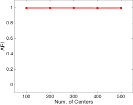
(a) ARI

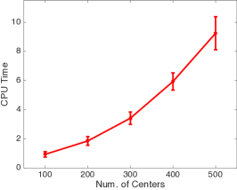
(b) CPU time

Figure 11: Clustering performance and CPU time against the number of kernel centers. Each point and error bar denote the average and standard deviation of (a) ARI and (b) CPU time over $50$ runs, respectively. The dataset used in this figure is the three Gaussian blobs in Section 5.1 when $(D,n)=(5,500)$

This appendix investigates clustering performance and computational costs of LSLDGC when the number of kernel centers is changed. We performed similar experiments in Section 5.1. In the experiments, datasets with the three Gaussian blobs (Fig.6(g)) were used.

Fig.11 shows that LSLDGC with a small number of kernel centers significantly reduces the computation costs without scarifying the clustering performance.

Appendix G Proof of Lemma 12

Proof  For $\epsilon^{\prime}$, the Cauchy-Schwarz inequality gives

$$|\widehat{g}_{j}(\bm{x})-g_{j}(\bm{x})|=|\langle\widehat{g}_{j}-g_{j},k(\cdot,\bm{x})\rangle_{\mathcal{H}}|\leq\|\widehat{g}_{j}-g_{j}\|_{\mathcal{H}}|k(\bm{x},\bm{x})|.$$

Since $k(\bm{x},\bm{x})$ is assumed to be finite,

$$\epsilon^{\prime}=\max_{j}\|\widehat{g}_{j}(\bm{x})-g_{j}(\bm{x})\|_{\infty}\leq O\left(\|\widehat{g}_{j}-g_{j}\|_{\mathcal{H}}\right) =O_{\mathrm{P}}\left(n^{-\min\left\{\frac{1}{4},\frac{\gamma}{2(\gamma+1)}\right\}}\right),$$ (55)

where we applied Theorem 1.

For $\epsilon^{\prime\prime}$, similar computation yields

$$|[\widehat{\mathbf{\Sigma}}^{-1}(\bm{x})]_{ij}-[\mathbf{\Sigma}^{-1}(\bm{x})]_{ij}|$$

$$=|-(\widehat{g}_{i}(\bm{x})\widehat{g}_{j}(\bm{x})-g_{i}(\bm{x})g_{j}(\bm{x}))+[\widehat{\bm{H}}(\bm{x})]_{ij}-[{\bm{H}}(\bm{x})]_{ij}|$$

$$\leq|\widehat{g}_{i}(\bm{x})\widehat{g}_{j}(\bm{x})-g_{i}(\bm{x})g_{j}(\bm{x})|+|[\widehat{\bm{H}}(\bm{x})]_{ij}-[{\bm{H}}(\bm{x})]_{ij}|$$

$$\leq|\widehat{g}_{i}(\bm{x})|\cdot|\widehat{g}_{j}(\bm{x})-g_{j}(\bm{x})|+|g_{j}(\bm{x})|\cdot|\widehat{g}_{i}(\bm{x})-g_{i}(\bm{x})|+|[\widehat{\bm{H}}(\bm{x})]_{ij}-[{\bm{H}}(\bm{x})]_{ij}|$$

$$\leq\left\{|g_{i}(\bm{x})|\cdot\|\widehat{g}_{j}-{g}_{j}\|_{\mathcal{H}}+|\widehat{g}_{j}(\bm{x})|\cdot\|\widehat{g}_{i}-{g}_{i}\|_{\mathcal{H}}+\|[\widehat{\bm{H}}]_{ij}-[{\bm{H}}]_{ij}\|_{\mathcal{H}}\right\}|k(\bm{x},\bm{x})|,$$

where we applied the following inequality on the fourth line:

$$|\widehat{g}_{i}(\bm{x})\widehat{g}_{j}(\bm{x})-g_{i}(\bm{x})g_{j}(\bm{x})| =|\widehat{g}_{i}(\bm{x})\widehat{g}_{j}(\bm{x})-\widehat{g}_{i}(\bm{x})g_{j}(\bm{x})+\widehat{g}_{i}(\bm{x})g_{j}(\bm{x})-g_{i}(\bm{x})g_{j}(\bm{x})|$$

$$=|\widehat{g}_{i}(\bm{x})(\widehat{g}_{j}(\bm{x})-g_{j}(\bm{x}))+g_{j}(\bm{x})(\widehat{g}_{i}(\bm{x})-g_{i}(\bm{x}))|$$

$$\leq|\widehat{g}_{i}(\bm{x})|\cdot|\widehat{g}_{j}(\bm{x})-g_{j}(\bm{x})|+|g_{j}(\bm{x})|\cdot|\widehat{g}_{i}(\bm{x})-g_{i}(\bm{x})|.$$

Thus, we obtain

$$\epsilon^{\prime\prime} =\max_{ij}\max_{\bm{x}}|[\widehat{\mathbf{\Sigma}}^{-1}(\bm{x})]_{ij}-[\mathbf{\Sigma}^{-1}(\bm{x})]_{ij}|$$

$$\leq\max_{ij}O\left(\max(\|\widehat{g}_{j}-{g}_{j}\|_{\mathcal{H}},\|\widehat{g}_{i}-{g}_{i}\|_{\mathcal{H}},\|[\widehat{\bm{H}}]_{ij}-[{\bm{H}}]_{ij}\|_{\mathcal{H}})\right)$$

$$=O_{\mathrm{P}}\left(n^{-\min\left\{\frac{1}{4},\frac{\gamma}{2(\gamma+1)}\right\}}\right),$$ (56)

where it follows from Theorem 1.

For $\epsilon^{\prime\prime\prime}$, we resort to the derivative reproducing property proved in Zhou (2008): For all $f\in\mathcal{H}$,

$$\partial_{j}f(\bm{x})=\langle f,\partial_{j}k(\cdot,\bm{x})\rangle_{\mathcal{H}}.$$

Using this relation, we obtain

$$|[\widehat{\mathbf{\Sigma}}^{-1\prime}(\bm{x})]_{ij}-[\mathbf{\Sigma}^{-1\prime}(\bm{x})]_{ij}| =|\partial_{j}[\text{vec}(\widehat{\mathbf{\Sigma}}^{-1}(\bm{x}))]_{i}-\partial_{j}[\text{vec}(\mathbf{\Sigma}^{-1}(\bm{x}))]_{i}|$$

$$=|\langle[\text{vec}(\widehat{\mathbf{\Sigma}}^{-1})]_{i}-[\text{vec}(\mathbf{\Sigma}^{-1})]_{i},\partial_{j}k(\cdot,\bm{x})\rangle_{\mathcal{H}}|$$

$$\leq\|\text{vec}(\widehat{\mathbf{\Sigma}}^{-1})]_{i}-[\text{vec}(\mathbf{\Sigma}^{-1})]_{i}\|_{\mathcal{H}}|\partial_{i}^{\prime}\partial_{i}k(\bm{x}^{\prime},\bm{x})|_{\bm{x}^{\prime}=\bm{x}}|,$$

where $\partial_{j}^{\prime}$ denote the derivative with respect to the $j$-th coordinate in $\bm{x}^{\prime}$. Since $|\partial_{j}^{\prime}\partial_{j}k|$ is assumed to be finite, (56) provides

$$\epsilon^{\prime\prime\prime} =\max_{ij}\max_{\bm{x}}|[\widehat{\mathbf{\Sigma}}^{-1\prime}(\bm{x})]_{ij}-[\mathbf{\Sigma}^{-1\prime}(\bm{x})]_{ij}|$$

$$\leq\max_{i}O\left(\|[\text{vec}(\widehat{\mathbf{\Sigma}}^{-1})]_{i}-[\text{vec}(\mathbf{\Sigma}^{-1})]_{i}\|_{\mathcal{H}}\right)$$

$$=O_{\mathrm{P}}\left(n^{-\min\left\{\frac{1}{4},\frac{\gamma}{2(\gamma+1)}\right\}}\right),$$

where the last equation comes from (56) because $[\text{vec}(\mathbf{\Sigma}^{-1})(\bm{x})]_{i}$ denotes a single element in $\mathbf{\Sigma}^{-1}(\bm{x})$.

References

- Arias-Castro et al. [2016] E. Arias-Castro, D. Mason, and B. Pelletier. On the estimation of the gradient lines of a density and the consistency of the mean-shift algorithm. Journal of Machine Learning Research, 17:1–28, 2016.
- Bache and Lichman [2013] K. Bache and M. Lichman. UCI machine learning repository, 2013. URL http://archive.ics.uci.edu/ml/.
- Beckner [1975] W. Beckner. Inequalities in Fourier analysis. Annals of Mathematics, 102(1):159–182, 1975.
- Beran [1976] R. Beran. Adaptive estimates for autoregressive processes. Annals of the Institute of Statistical Mathematics, 28(1):77–89, 1976.
- Bowman [1984] A. Bowman. An alternative method of cross-validation for the smoothing of density estimates. Biometrika, 71(2):353–360, 1984.
- Carreira-Perpiñán [2000] M. Carreira-Perpiñán. Reconstruction of sequential data with probabilistic models and continuity constraints. In Advances in neural information processing systems, pages 414–420, 2000.
- Carreira-Perpiñán [2001] M. Carreira-Perpiñán. Continuous latent variable models for dimensionality reduction and sequential data reconstruction. PhD thesis, University of Sheffield, 2001. (Section 7.3).
- Carreira-Perpiñán [2006] M. Carreira-Perpiñán. Acceleration strategies for Gaussian mean-shift image segmentation. In Proceedings of IEEE Computer Society Conference on Computer Vision and Pattern Recognition (CVPR), pages 1160–1167, 2006.
- Carreira-Perpiñán [2007] M. Carreira-Perpiñán. Gaussian mean-shift is an EM algorithm. IEEE Transactions on Pattern Analysis and Machine Intelligence, 29(5):767–776, 2007.
- Carreira-Perpiñán [2015] M. Carreira-Perpiñán. A review of mean-shift algorithms for clustering. arXiv preprint arXiv:1503.00687, 2015.
- Chen et al. [2015a] Y.-C. Chen, C. R. Genovese, S. Ho, and L. Wasserman. Optimal ridge detection using coverage risk. In Advances in Neural Information Processing Systems, pages 316–324, 2015a.
- Chen et al. [2015b] Y.-C. Chen, C. R. Genovese, and L. Wasserman. Asymptotic theory for density ridges. The Annals of Statistics, 43(5):1896–1928, 2015b.
- Chen et al. [2016a] Y.-C. Chen, C. Genovese, R. Tibshirani, and L. Wasserman. Nonparametric modal regression. The Annals of Statistics, 44(2):489–514, 2016a.
- Chen et al. [2016b] Y.-C. Chen, C. Genovese, and L. Wasserman. A comprehensive approach to mode clustering. Electronic Journal of Statistics, 10(1):210–241, 2016b.
- Chen et al. [2016c] Y.-C. Chen, S. Ho, P. Freeman, C. Genovese, and L. Wasserman. Cosmic web reconstruction through density ridges: Method and algorithm. Monthly Notices of the Royal Astronomical Society, 454(1):1140–1156, 2016c.
- Cheng [1995] Y. Cheng. Mean shift, mode seeking, and clustering. IEEE Transactions on Pattern Analysis and Machine Intelligence, 17(8):790–799, 1995.
- Collins [2003] R. T. Collins. Mean-shift blob tracking through scale space. In Proceedings of IEEE Computer Society Conference on Computer Vision and Pattern Recognition (CVPR), pages 234–240, 2003.
- Comaniciu and Meer [2002] D. Comaniciu and P. Meer. Mean shift: A robust approach toward feature space analysis. IEEE Transactions on Pattern Analysis and Machine Intelligence, 24(5):603–619, 2002.
- Comaniciu et al. [2000] D. Comaniciu, V. Ramesh, and P. Meer. Real-time tracking of non-rigid objects using mean shift. In Proceedings of IEEE Conference on Computer Vision and Pattern Recognition (CVPR), pages 142–149, 2000.
- Cox [1985] D. D. Cox. A penalty method for nonparametric estimation of the logarithmic derivative of a density function. Annals of the Institute of Statistical Mathematics, 37(1):271–288, 1985.
- Dempster et al. [1977] A. P. Dempster, N. M. Laird, and D. B. Rubin. Maximum likelihood from incomplete data via the EM algorithm. Journal of the royal statistical society. Series B (methodological), 39(1):1–38, 1977.
- Drinkwater et al. [2004] M. J. Drinkwater, Q. A. Parker, D. Proust, E. Slezak, and H. Quintana. The large scale distribution of galaxies in the shapley supercluster. Publications of the Astronomical Society of Australia, 21(1):89–96, 2004.
- Duong et al. [2008] T. Duong, A. Cowling, I. Koch, and M. P. Wand. Feature significance for multivariate kernel density estimation. Computational Statistics & Data Analysis, 52(9):4225–4242, 2008.
- Eberly [1996] D. Eberly. Ridges in Image and Data Analysis. Springer, 1996.
- Einbeck and Tutz [2006] J. Einbeck and G. Tutz. Modelling beyond regression functions: an application of multimodal regression to speed–flow data. Journal of the Royal Statistical Society: Series C (Applied Statistics), 55(4):461–475, 2006.
- Fashing and Tomasi [2005] M. Fashing and C. Tomasi. Mean shift is a bound optimization. IEEE Transactions on Pattern Analysis and Machine Intelligence, 27(3):471–474, 2005.
- Forina et al. [1983] M. Forina, C. Armanino, S. Lanteri, and E. Tiscornia. Classification of olive oils from their fatty acid composition. In Food research and data analysis, pages 189–214. Applied Science Publishers, London, 1983.
- Fukumizu et al. [2007] K. Fukumizu, F. Bach, and A. Gretton. Statistical consistency of kernel canonical correlation analysis. Journal of Machine Learning Research, 8:361–383, 2007.
- Fukunaga and Hostetler [1975] K. Fukunaga and L. Hostetler. The estimation of the gradient of a density function, with applications in pattern recognition. IEEE Transactions on Information Theory, 21(1):32–40, 1975.
- Gasser et al. [1998] T. Gasser, P. Hall, and B. Presnell. Nonparametric estimation of the mode of a distribution of random curves. Journal of the Royal Statistical Society: Series B (Statistical Methodology), 60(4):681–691, 1998.
- Genovese et al. [2014] C. R. Genovese, M. Perone-Pacifico, I. Verdinelli, and L. Wasserman. Nonparametric ridge estimation. The Annals of Statistics, 42(4):1511–1545, 2014.
- Genovese et al. [2016] C. R. Genovese, M. Perone-Pacifico, I. Verdinelli, and L. Wasserman. Non-parametric inference for density modes. Journal of the Royal Statistical Society: Series B (Statistical Methodology), 78(1):99–126, 2016.
- Ghassabeh [2013] Y. A. Ghassabeh. On the convergence of the mean shift algorithm in the one-dimensional space. Pattern Recognition Letters, 34(12):1423–1427, 2013.
- Ghassabeh et al. [2013] Y. A. Ghassabeh, T. Linder, and G. Takahara. On some convergence properties of the subspace constrained mean shift. Pattern Recognition, 46(11):3140–3147, 2013.
- Godtliebsen et al. [2002] F. Godtliebsen, J. S. Marron, and P. Chaudhuri. Significance in scale space for bivariate density estimation. Journal of Computational and Graphical Statistics, 11(1):1–21, 2002.
- Hubert and Arabie [1985] L. Hubert and P. Arabie. Comparing partitions. Journal of Classification, 2(1):193–218, 1985.
- Hyvärinen [2005] A. Hyvärinen. Estimation of non-normalized statistical models by score matching. Journal of Machine Learning Research, 6:695–709, 2005.
- Kain and Macon [1998] A. Kain and M. W. Macon. Spectral voice conversion for text-to-speech synthesis. In Proceedings of IEEE International Conference on Acoustics, Speech and Signal Processing, pages 285–288, 1998.
- Kanamori et al. [2009] T. Kanamori, S. Hido, and M. Sugiyama. A least-squares approach to direct importance estimation. Journal of Machine Learning Research, 10:1391–1445, 2009.
- Kanamori et al. [2012] T. Kanamori, T. Suzuki, and M. Sugiyama. Statistical analysis of kernel-based least-squares density-ratio estimation. Machine Learning, 86(3):335–367, 2012.
- Kpotufe [2017] S. Kpotufe. Lipschitz density-ratios, structured data, and data-driven tuning. In Proceedings of the 20th International Conference on Artificial Intelligence and Statistics (AISTATS), volume 54, pages 1320–1328, 2017.
- Li et al. [2007] X. Li, Z. Hu, and F. Wu. A note on the convergence of the mean shift. Pattern recognition, 40(6):1756–1762, 2007.
- MacQueen [1967] J. B. MacQueen. Some methods for classification and analysis of multivariate observations. In Proceedings of the 5th Berkeley Symposium on Mathematical Statistics and Probability, volume 1, pages 281–297, Berkeley, CA, USA, 1967. University of California Press.
- Melnykov and Maitra [2010] V. Melnykov and R. Maitra. Finite mixture models and model-based clustering. Statistics Surveys, 4:80–116, 2010.
- Micchelli et al. [2006] C. A. Micchelli, Y. Xu, and H. Zhang. Universal kernels. Journal of Machine Learning Research, 7:2651–2667, 2006.
- Ng et al. [2001] A. Y. Ng, M. I. Jordan, and Y. Weiss. On spectral clustering: Analysis and an algorithm. In Advances in Neural Information Processing Systems, volume 14, pages 849–856, 2001.
- Nguyen et al. [2008] X. Nguyen, M. J. Wainwright, and M. I. Jordan. Estimating divergence functionals and the likelihood ratio by penalized convex risk minimization. In Advances in neural information processing systems (NIPS), pages 1089–1096, 2008.
- Ozertem and Erdogmus [2011] U. Ozertem and D. Erdogmus. Locally defined principal curves and surfaces. Journal of Machine Learning Research, 12:1249–1286, 2011.
- Parzen [1962] E. Parzen. On estimation of a probability density function and mode. The Annals of Mathematical Statistics, 33(3):1065–1076, 1962.
- Pulkkinen [2015] S. Pulkkinen. Ridge-based method for finding curvilinear structures from noisy data. Computational Statistics & Data Analysis, 82:89–109, 2015.
- Sager and Thisted [1982] T. W. Sager and R. A. Thisted. Maximum likelihood estimation of isotonic modal regression. The Annals of Statistics, 10(3):690–707, 1982.
- Sasaki et al. [2014] H. Sasaki, A. Hyvärinen, and M. Sugiyama. Clustering via mode seeking by direct estimation of the gradient of a log-density. In Machine Learning and Knowledge Discovery in Databases Part III- European Conference, ECML/PKDD 2014, volume 8726, pages 19–34, 2014.
- Sasaki et al. [2015] H. Sasaki, Y. K. Noh, and M. Sugiyama. Direct density-derivative estimation and its application in KL-divergence approximation. In Proceedings of the 18th International Conference on Artificial Intelligence and Statistics (AISTATS), pages 809–818, 2015.
- Sasaki et al. [2016] H. Sasaki, Y. Ono, and M. Sugiyama. Modal regression via direct log-density gradient estimation. In Proceedings of the 23th International Conference on Neural Information Processing (ICONIP), volume 9948, pages 108–116. Springer, 2016.
- Sasaki et al. [2017] H. Sasaki, T. Kanamori, and M. Sugiyama. Estimating density ridges by direct estimation of density-derivative-ratios. In Proceedings of the 20th International Conference on Artificial Intelligence and Statistics (AISTATS), volume 54, pages 204–212, 2017.
- Sheather [2004] S. J. Sheather. Density estimation. Statistical Science, 19(4):588–597, 2004.
- Shi and Malik [2000] J. Shi and J. Malik. Normalized cuts and image segmentation. IEEE Transactions on Pattern Analysis and Machine Intelligence, 22(8):888–905, 2000.
- Silverman [1986] B. Silverman. Density Estimation for Statistics and Data Analysis. CRC press, 1986.
- Sriperumbudur et al. [2013] B. Sriperumbudur, K. Fukumizu, A. Gretton, and A. Hyvärinen. Density estimation in infinite dimensional exponential families. arXiv preprint arXiv:1312.3516 (ver.3), 2013.
- Sriperumbudur et al. [2017] B. Sriperumbudur, K. Fukumizu, A. Gretton, A. Hyvärinen, and R. Kumar. Density estimation in infinite dimensional exponential families. Journal of Machine Learning Research, 18(57):1–59, 2017.
- Steinwart and Christmann [2008] I. Steinwart and A. Christmann. Support vector machines. Springer, 2008.
- Strang [1991] G. Strang. Calculus. Wellesley-Cambridge Press, 1991.
- Su et al. [2013] J. Su, A. Srivastava, and F. Huffer. Detection, classification and estimation of individual shapes in 2D and 3D point clouds. Computational Statistics & Data Analysis, 58:227–241, 2013.
- Sugiyama et al. [2008] M. Sugiyama, S. Nakajima, H. Kashima, P. V. Buenau, and M. Kawanabe. Direct importance estimation with model selection and its application to covariate shift adaptation. In Advances in neural information processing systems (NIPS), pages 1433–1440, 2008.
- Sugiyama et al. [2012] M. Sugiyama, T. Suzuki, and T. Kanamori. Density Ratio Estimation in Machine Learning. Cambridge University Press, 2012.
- Sugiyama et al. [2014] M. Sugiyama, G. Niu, M. Yamada, M. Kimura, and H. Hachiya. Information-maximization clustering based on squared-loss mutual information. Neural Computation, 26(1):84–131, 2014.
- Tao et al. [2007] W. Tao, H. Jin, and Y. Zhang. Color image segmentation based on mean shift and normalized cuts. IEEE Transactions on Systems, Man, and Cybernetics, Part B: Cybernetics, 37(5):1382–1389, 2007.
- Tsybakov [2009] A. B. Tsybakov. Introduction to Nonparametric Estimation. Springer, 2009.
- Turney [1993] P. D. Turney. Robust classification with context-sensitive features. In Proceedings of the 6th international conference on Industrial and engineering applications of artificial intelligence and expert systems, pages 268–276. Gordon & Breach Science Publishers, 1993.
- Wang et al. [2004] J. Wang, B. Thiesson, Y. Xu, and M. Cohen. Image and video segmentation by anisotropic kernel mean shift. In Proceedings of European Conference on Computer Vision (ECCV), pages 238–249, 2004.
- Wasserman [2018] L. Wasserman. Topological data analysis. Annual Review of Statistics and Its Application, 5:501–532, 2018.
- Wendland [2004] H. Wendland. Scattered data approximation. Cambridge university press, 2004.
- Yao et al. [2012] W. Yao, B. G. Lindsay, and R. Li. Local modal regression. Journal of nonparametric statistics, 24(3):647–663, 2012.
- You et al. [2011] S. You, E. Bas, D. Erdogmus, and J. Kalpathy-Cramer. Principal curved based retinal vessel segmentation towards diagnosis of retinal diseases. In Proceedings of IEEE International Conference on Healthcare Informatics, Imaging and Systems Biology (HISB), pages 331–337, 2011.
- Zhou [2008] D. Zhou. Derivative reproducing properties for kernel methods in learning theory. Journal of Computational and Applied Mathematics, 220(1-2):456–463, 2008.