Local Nonparametric Estimation for Second-Order Jump-Diffusion Model Using Gamma Asymmetric Kernels

Abstract

This paper discusses the local linear smoothing to estimate the unknown first and second infinitesimal moments in second-order jump-diffusion model based on Gamma asymmetric kernels. Under the mild conditions, we obtain the weak consistency and the asymptotic normality of these estimators for both interior and boundary design points. Besides the standard properties of the local linear estimation such as simple bias representation and boundary bias correction, the local linear smoothing using Gamma asymmetric kernels possess some extra advantages such as variable bandwidth, variance reduction and resistance to sparse design, which is validated through finite sample simulation study. Finally, we employ the estimators for the return of some high frequency financial data.

JEL classification: C13, C14, C22.

Keywords: Return model; Variable bandwidth; Variance reduction; Resistance to sparse design; High frequency financial data.

1 Introduction

Continuous-time models are widely used in economics and finance, such as interest rate and etc., especially the continuous-time diffusion processes with jumps. Jump-diffusion process $X_{t}$ is represented by the following stochastic differential equation:

$$dX_{t}=\mu(X_{t-})dt+\sigma(X_{t-})dW_{t}+\int_{\mathscr{E}}c(X_{t-},z)r(\omega,dt,dz),$$ (1)

which can accommodate the impact of sudden and large shocks to financial markets. Johannes [26] provided the statistical and economic role of jumps in continuous-time interest rate models. However, in empirical finance or physics the current observation usually behaves as the cumulation of all past perturbation such as stock prices by means of returns and exchange rates in Nicolau [34] and the velocity of the particle on the surface of a liquid in Rogers and Williams [39]. Furthermore, in the research field involved with model (1), the scholars mainly considered it for the price of a asset not for the returns of the price. As mentioned in Campbell, Lo and MacKinlay [5], return series of an asset are a complete and scale-free summary of the investment opportunity for average investors, and are easier to handle than price series due to their more attractive statistical properties.

For characterizing this integrated economic phenomenon, moreover, and the return series, Nicolau [33] considered the promising continuous second-order diffusion process (2), which is motivated by unit root processes under the discrete framework of Park and Phillips [36],

$$\left\{\begin{array}[]{ll}dY_{t}=X_{t}dt,\\ dX_{t}=\mu(X_{t})dt+\sigma(X_{t})dW_{t},\end{array}\right.$$ (2)

which may be an alternative model to describe the dynamic of some financial data. Considering empirical properties of return series such as higher peak, fatter tails and etc., here we extend the continuous autoregression of order two (2) to a discontinuous and realistic case with jumps for return series based on model (1), noted as the second-order jump-diffusion process (3) to represent integrated and differentiated processes,

$$\left\{\begin{array}[]{ll}dY_{t}=X_{t-}dt,\\ dX_{t}=\mu(X_{t-})dt+\sigma(X_{t-})dW_{t}+\int_{\mathscr{E}}c(X_{t-},z)r(\omega,dt,dz),\end{array}\right.$$ (3)

where $W_{t}$ is a standard Brownian motion, $\mu(\cdot)$ and $\sigma(\cdot)$ are the infinitesimal conditional drift and variance respectively, $\mathscr{E}=\mathbb{R}\setminus\{0\},$ $r(\omega,dt,dz)=(p-q)(dt,dz),~{}p(dt,dz)$ is a time-homogeneous Poisson random measure on $\mathbb{R}_{+}\times\mathbb{R}$ independent of $W_{t}$, and $q(dt,dz)$ is its intensity measure, that is, $E[p(dt,dz)]=q(dt,dz)=f(z)dzdt$, $f(z)$ is its Lévy density. For empirical financial data, $X_{t}$ represents the continuously compounded return of underlying assets, $Y_{t}$ denotes the asset price by means of the cumulation of the returns plus initial asset value. Note that model (3) is neither a special case of a two-dimensional stochastic differential equation nor a stochastic volatility model without noise in the first coordinate. It is essentially the linear version of the following nonlinear stochastic jump-diffusion equation of order two considered in Özden and Ünal [35]

$$d\dot{X}_{t}=f(t,X_{t},\dot{X}_{t})dt+g(t,X_{t},\dot{X}_{t})dW_{t}+j(t,X_{t},\dot{X}_{t})dN_{t},$$ (4)

where $dN_{t}$ denotes the infinitesimal increment of Poisson process and $f,g,j$ are the coefficient functions.

Model (3) can be used commonly in empirical financial for at least four reasons. Firstly, in contrary to the usual models for the price of a asset such as model (1), model (3) overcomes the difficulties associated with the nondifferentiability of a Brownian motion, which can model integrated and differentiated diffusion processes for the cumulation of all past perturbations in modern econometric phenomena (similarly as unit root processes in a discrete framework). Furthermore, the model (3) can accommodate nonstationary original process and be made stationary by linear combinations such as differencing, which is a more widely adopted technique used in empirical financial. We have verified this property through the Augmented Dickey-Fuller test statistic for the sampling time series before and after the difference in the empirical analysis part. Secondly, compared with the model (2), model (3) accommodates the impact by macroeconomic announcements and a dramatic interest rate cut by the Federal Reserve in combination with jump component. It has been testified the existence of jumps modeling by (2) or (3) for real financial data through the test statistic proposed in Barndorff-Nielsen and Shephard [3] in empirical analysis part. Thirdly, model (3) can directly characterize the returns with heavy tail (or the log return) of a asset to specify general properties for returns (such as stationarity in the mean and weakness in the autocorrelation et al.) more easily than a diffusion univariate process for the price of a asset (such as stock prices and nominal exchange rates). Fourthly, the integro-differential jump-diffusion model (3) can also be employed in finance for integrated volatility in stochastic volatility models with jumps.

For model (3), Özden and Ünal [35] gave the linearization criterion in terms of coefficients for transforming a nonlinear stochastic differential equations into linear ones via invertible stochastic mappings in order to solve exact solutions. However, we do not know beforehand the specific form of the model coefficients to verify these criteria in practical applications, so we should statistically estimate the unknown coefficients in model (3) for modeling the economic and financial phenomena based on the observations. For continuous case (2), Gloter [16] [17] and Ditlevsen and Sørensen [12] presented the parametric and semiparametric estimation from a discretely observed samples. Recently, an inordinate amount of attention has been focused on nonparametric methods in econometrics due to the flexibility for handling the nonlinear conditional moment estimation, not assuming its expression in contrary to parametric estimation. Nicolau [33] and Wang and Lin [47] analyzed the local nonparametric estimations using symmetric kernel and Hanif [22] studied Nadaraya-Watson estimators using Gamma asymmetric kernel. For model (3), Song [43] considered Nadaraya-Watson estimators for the unknown coefficients using Gaussian symmetric kernel in high frequency data.

In the context of nonparametric estimator with finite-dimensional auxiliary variables, local polynomial smoothing become an effective smoothing method, which has excellent properties of full asymptotic minimax efficiency achievement and boundary bias correction automatically, one can refer to Fan and Gijbels [14] for better review. In general, the popular choices for kernels in application of local polynomial estimators are symmetric and compact. However, local nonparametric estimation constructed with symmetric kernels for the nonnegative variables or nonnegative part of the underlying variables in economics and finance is not approximate for the region near the origin without a boundary correction. Furthermore, for finite sample size, Seifert and Gasser [41] found the problem of unbounded variance in sparse regions for local polynomial smoothing employing a compact kernel and proposed local increase of bandwidth in sparse regions of the design to add more information to reduce the corresponding variability. Fortunately, local nonparametric smoothing using asymmetric kernels can effectively solve the above two major problems for nonparametric estimation.

Besides the usual standard properties of the local linear estimation such as the simple bias representation and boundary bias correction, the local linear smoothing using Gamma asymmetric kernel with unbounded support $[0,\infty)$ have some extra benefits as follows such as variable bandwidth, variance reduction and resistance to sparse design. Firstly, the Gamma asymmetric kernel is a kind of adaptive and flexible smoothing, whose curve shapes can vary with the smoothing parameter and the location of the design point similar as the variable bandwidth methods, which is illustrated in FIG 1 for a fixed smoothing parameter. As mentioned in Gospodinov and Hirukawa [18], unlike the variable bandwidth methods, the smoothing method constructed with Gamma asymmetric kernel is achieved by only a single smoothing parameter. Secondly, when the support of Gamma asymmetric kernel matches the support of the curve of the function to be estimated, and the curve has sparse regions, the finite variance of the curve estimation decreases due to the fact that their variances vary along with the location of the design point $x$ and the increase of the effective sample size for estimation. Thirdly, Gamma asymmetric kernels are free from boundary bias (allowing a larger bandwidth to pool more data) and achieve the optimal rate of convergence in mean square error within the class of nonnegative kernel estimators with order two. In conclusion, asymmetric kernels is a combination of a boundary correction device and a “variable bandwidth” method. For a review of application using asymmetric kernels, one should refer to Chen [7] [8] to estimate densities, Chen [9] to estimate a regression curve with bounded support, Bouezmarni and Scaillet [4] to apply the asymmetric kernel density estimators to income data, Kristensen [29] to consider the realized integrated volatility estimation, Gospodinov and Hirukawa [18] to propose an asymmetric kernel-based method for scalar diffusion models of spot interest rates, compared with Stanton [46], to show that asymmetric kernel smoothing is expected to reduce substantially both the bias near the origin and the bias that occurs for high values in the estimation of the drift coefficient. Hanif [21] addressed local linear estimation using Gamma asymmetric kernels for the infinitesimal moments in model (1).

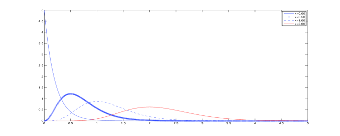
Figure 1: Shapes of the Gamma function with a fixed smoothing parameter (0.2) at various design points ($x=0.0,0.5,1.0,2.0$)

For model (3), although Chen and Zhang [11] discussed the local linear estimators for the unknown functions $\mu(x)$ and $\sigma^{2}(x)+\int_{\mathscr{E}}c^{2}(x,z)f(z)dz$ based on symmetric kernels. More previous works focused on the simplification for the bias representation of the estimator, while less research was considered deeply for the reduction in variance. Gouriéroux and Monfort [19] and Jones and Henderson [27] argued that unlike the symmetric kernels case, the empirical data $X_{t}$ point and the design point $x$ in asymmetric kernels case are not exchangeable. Hence, we cannot establish the asymptotic theorems for the Gamma kernel estimators of unknown coefficients in model (3) by the means of the similar approach as that in Bandi and Nguyen [2] and Chen and Zhang [11]. In this paper, we will propose local linear estimators of $\mu(x)$ and $\sigma^{2}(x)+\int_{\mathscr{E}}c^{2}(x,z)f(z)dz$ in model (3) using Gamma asymmetric kernels for both bias correction, especially for boundary point near the origin, and variance reduction, especially for sparse design point far away from the origin.

For convenience, we note $X_{i}=X_{i\Delta_{n}}$, $\widetilde{X}_{i}=\widetilde{X}_{i\Delta_{n}}$ in the remainder of this paper which is organized as follows. In Section 2, we propose local linear estimators with asymmetric kernels and some ordinary assumptions for model (3). We present the asymptotic results in Section 3. Section 4 presents the finite sample performance through Monte Carlo simulation study. The estimators are illustrated empirically in Section 5. Section 6 concludes. Some technical lemmas and the main proofs are explicitly shown in Section 7.

2 Local Linear Estimators with Asymmetric Kernels and Assumptions

According to the asymmetric kernels used in Chen [8], the Gamma kernel function is defined as

$$K_{G(x/h+1,h)}(u)=\frac{u^{x/h}\exp(-u/h)}{h^{x/h+1}\Gamma(x/h+1)}~{}~{}0\leq u\leq\infty,$$ (5)

where $\Gamma(m)=\int^{\infty}_{0}{y^{m-1}\exp(-y)dy},~{}m>0$ is the Gamma function and $h$ is the smoothing parameter. Note that we use modified Gamma kernel function $K_{G(x/h+1,h)}(u)$ instead of $K_{G(x/h,h)}(u)$ due to the fact $K_{G(x/h,h)}(u)$ is unbounded near at $x=0.$ As is shown in Figure 1, the Gamma function has shapes varying with the design point $x,$ which changes the amount of smoothing applied by the asymmetric kernels since the variance $xh+h^{2}$ of $K_{G(x/h+1,h)}(u)$ is increasing as $x$ away from the boundary. Additionally, as discussed in Bouezmarni and Scaillet [4] the consistency of gamma kernel estimator holds even though the true density is unbounded at $x=0.$ Statistically and theoretically, since the density of Gamma distribution has support $[0,\infty)$, the Gamma kernel function does not generate boundary bias for nonnegative variables or nonnegative part of underlying variables. Furthermore, the asymptotic variance of the nonparametric Gamma kernel estimation depends on the design point $x,$ which yields the optimal rate of convergence in mean integrated squared error of nonnegative kernels.

Different from model (1), nonparametric estimations constructed for the coefficients in second-order jump-diffusion model (3) give rise to new challenges for two main reasons.

On the one hand, we usually get observations $\{Y_{i\Delta_{n}};i=1,2,\cdot\cdot\cdot\}$ rather than $\{X_{i\Delta_{n}};i=1,2,\cdot\cdot\cdot\}.$ The value of $X_{t_{i}}$ cannot be obtained from $Y_{t_{i}}=Y_{0}+\int_{0}^{t_{i}}X_{s}ds$ in a fixed sample intervals. Additionally, nonparametric estimations of the unknown qualities in model (3) cannot in principle be constructed on the observations $\{Y_{i\Delta_{n}};i=1,2,\cdot\cdot\cdot\}$ due to the unknown conditional distribution of $Y$. As Nicolau [33] showed, with observations $\{Y_{i\Delta_{n}};i=1,2,\cdot\cdot\cdot\}$ and given that

$$Y_{{i\Delta_{n}}}-Y_{{(i-1)\Delta_{n}}}=\int_{(i-1)\Delta_{n}}^{i\Delta_{n}}X_{u}du,$$

we can obtain an approximation value of $X_{i\Delta_{n}}$ by

$$\widetilde{X}_{i\Delta_{n}}=\frac{Y_{i\Delta_{n}}-Y_{(i-1)\Delta_{n}}}{\Delta_{n}}.$$ (6)

On the other hand, the Markov properties for statistical inference of unknown qualities in model (3) based on the samples $\{\widetilde{X}_{i\Delta_{n}};i=1,2,\cdot\cdot\cdot\}$ should be built, which are infinitesimal conditional expectations characterized by infinitesimal operators. Fortunately, under Lemma 1 we can build the following infinitesimal conditional expectations for model (3)

$$E[\frac{\widetilde{X}_{(i+1)\Delta_{n}}-\widetilde{X}_{i\Delta_{n}}}{\Delta_{n}}|\mathscr{F}_{(i-1)\Delta_{n}}]=\mu(X_{(i-1)\Delta_{n}})+O_{p}(\Delta_{n}),$$ (7)

$$E[\frac{(\widetilde{X}_{(i+1)\Delta_{n}}-\widetilde{X}_{i\Delta_{n}})^{2}}{\Delta_{n}}|\mathscr{F}_{(i-1)\Delta_{n}}]=\frac{2}{3}\sigma^{2}(X_{(i-1)\Delta_{n}})+\frac{2}{3}\int_{\mathscr{E}}c^{2}(X_{(i-1)\Delta_{n}},z)f(z)dz+O_{p}(\Delta_{n}).$$ (8)

where $\mathscr{F}_{t}=\sigma\{X_{s},s\leq t\}$. One can refer to Appendix A in Song, Lin and Wang [45] for detailed calculations.

Under $\{\widetilde{X}_{i\Delta_{n}};i=0,1,2,\cdot\cdot\cdot\}$, we construct local linear estimators for the unknown coefficients in model (3) based on equations (7) and (8). We consider the following weighted local linear regression to estimate $\mu(x)$ and $M(x)=\sigma^{2}(x)+\int_{\mathscr{E}}c(x,z)f(z)dz$ using asymmetric Gamma kernel, respectively:

$$\arg\min_{a,b}\sum_{i=1}^{n}\Big{(}\frac{\widetilde{X}_{(i+1)\Delta_{n}}-\widetilde{X}_{i\Delta_{n}}}{\Delta_{n}}-a-b(\widetilde{X}_{i\Delta_{n}}-x)\Big{)}^{2}K_{G(x/h+1,h)}\big{(}\widetilde{X}_{(i-1)\Delta_{n}}\big{)},$$ (9)

$$\arg\min_{a,b}\sum_{i=1}^{n}\Big{(}\frac{\frac{3}{2}(\widetilde{X}_{(i+1)\Delta_{n}}-\widetilde{X}_{i\Delta_{n}})^{2}}{\Delta_{n}}-a-b(\widetilde{X}_{i\Delta_{n}}-x)\Big{)}^{2}K_{G(x/h+1,h)}\big{(}\widetilde{X}_{(i-1)\Delta_{n}}\big{)},$$ (10)

where $K_{G(x/h+1,h)}(\cdot)$ is the asymmetric Gamma kernel function.

The solutions for $a$ to (9) and (10) as follows are respectively the local linear estimators of $\mu(x)$ and $M(x)=\sigma^{2}(x)+\int_{\mathscr{E}}c(x,z)f(z)dz,$

$$\hat{\mu}_{n}(x)=\frac{\sum_{i=1}^{n}\omega_{i-1}\Big{(}\frac{\widetilde{X}_{i+1}-\widetilde{X}_{i}}{\Delta_{n}}\Big{)}}{\sum_{i=1}^{n}\omega_{i-1}},$$ (11)

$$\hat{M}_{n}(x)=\frac{\sum_{i=1}^{n}\omega_{i-1}\frac{3}{2}\frac{(\widetilde{X}_{i+1}-\widetilde{X}_{i})^{2}}{\Delta_{n}}}{\sum_{i=1}^{n}\omega_{i-1}}$$ (12)

where

$$\omega_{i-1} = K_{G(x/h+1,h)}\big{(}\widetilde{X}_{i-1}\big{)}(\sum_{j=1}^{n}K_{G(x/h+1,h)}\big{(}\widetilde{X}_{j-1}\big{)}(\widetilde{X}_{j}-x)^{2}$$

$$-(\widetilde{X}_{i}-x)\sum_{j=1}^{n}K_{G(x/h+1,h)}\big{(}\widetilde{X}_{j-1}\big{)}(\widetilde{X}_{j}-x)).$$

There are some differences between the estimators given in this paper and the local linear estimators for the coefficients of model (1) in Hanif [21]. In (9) and (10) the observations in $(\widetilde{X}_{i}-x)$ and $K(\widetilde{X}_{i-1})$ are different for the model (3) which is more complex than the one in Hanif [21], because we need to calculate some meaningful conditional expect values of the estimators in the detailed proof by means of the method introduced by Nicolau [33], but cannot obtain the desired result if they are identical. Fortunately, $\widetilde{X}_{i}$ and $\widetilde{X}_{i-1}$ can both approximate the value of $X_{i-1}$, which guarantees the desired result in the article reasonably from the result in Hanif [21]. However, the local linear smoothing constructed in this paper cannot be extended to the local polynomial cases, which needs more than two values to approximate $X_{(i-1)\Delta_{n}}.$

We now present some assumptions used in the paper. In what follows, let $\mathscr{D}=(l,u)$ with $l\geq-\infty$ and $u\leq\infty$ denote the admissible range of the process $X_{t},$ $K$ denotes $K_{G(x/h+1,h)}.$

Assumption 1

(i) (Local Lipschitz continuity)  For each $n\in\mathbb{N},$ there exist a constant $L_{n}$ and a function $\zeta_{n}~{}:~{}\mathscr{E}\rightarrow\mathbb{R}_{+}$ with $\int_{\mathscr{E}}\zeta_{n}^{2}(z)f(z)dz<\infty$ such that, for any $|x|\leq n,|y|\leq n,~{}z\in\mathscr{E}$,

$$|\mu(x)-\mu(y)|+|\sigma(x)-\sigma(y)|\leq L_{n}|x-y|,~{}~{}~{}|c(x,z)-c(y,z)|\leq\zeta_{n}(z)|x-y|.$$

(ii) (Linear growthness)  For each $n\in\mathbb{N}$, there exist $\zeta_{n}$ as above and $C$, such that for all $x\in\mathbb{R},~{}z\in\mathscr{E}$,

$$|\mu(x)|+|\sigma(x)|\leq C(1+|x|),~{}|c(x,z)|\leq\zeta_{n}(z)(1+|x|).$$

Remark 1

Assumption 1 guarantees the existence and uniqueness of a solution to $X_{t}$ in Eq. (1) on the probability space $(\Omega,\mathscr{F},P)$, see Jacod and Shiryayev [25].

Assumption 2

The process $X_{t}$ is ergodic and stationary with a finite invariant measure $\phi(x)$. Furthermore, The process $X_{t}$ is $\rho-$mixing with $\sum_{i\geq 1}\rho(i\Delta_{n})=O(\frac{1}{\Delta_{n}^{\alpha}}),~{}n\rightarrow\infty,$ where $\alpha<\frac{1}{2}.$

Remark 2

The hypothesis that $X_{t}$ is a stationary process is obviously a plausible assumption because for major integrated time series data, a simple differentiation generally assures stationarity. The same condition yielding information on the rate of decay of $\rho-$mixing coefficients for $X_{t}$ was mentioned the Assumption 3 in Gugushvili and Spereij [20].

Assumption 3

For any 2 $\leq i$ $\leq n$, $g$ is a differentiable function on $\mathbb{R}$ and $\xi_{n,i}=\theta X_{(i-1)\Delta_{n}}+(1-\theta)\widetilde{X}_{(i-1)\Delta_{n}}$, $0\leq\theta\leq 1,$ the conditions hold:

(i)   $\lim_{h\rightarrow 0}E\big{[}~{}|hK^{{}^{\prime}}(\xi_{n,i})g(X_{(i-1)\Delta_{n}})|\big{]}<\infty,$

(ii)  $\lim_{h\rightarrow 0}h^{1/2}E\big{[}~{}|h^{2}K^{{}^{\prime}2}(\xi_{n,i})g(X_{(i-1)\Delta_{n}})|\big{]}<\infty$ for “interior x”,

(iii) $\lim_{h\rightarrow 0}hE\big{[}~{}|h^{2}K^{{}^{\prime}2}(\xi_{n,i})g(X_{(i-1)\Delta_{n}})|\big{]}<\infty$ for “boundary x”.

Remark 3

According to the procedure for assumption 3 in Appendix (7.1), we can easily deduce the following results:

(i)   $\lim_{h\rightarrow 0}E\big{[}~{}|K(X_{(i-1)\Delta_{n}})g(X_{(i-1)\Delta_{n}})|\big{]}<\infty;$

(ii)  $\lim_{h\rightarrow 0}h^{1/2}E\big{[}~{}|K^{2}(X_{(i-1)\Delta_{n}})g(X_{(i-1)\Delta_{n}})|\big{]}<\infty$ for “interior x”;

(iii) $\lim_{h\rightarrow 0}hE\big{[}~{}|K^{2}(X_{(i-1)\Delta_{n}})g(X_{(i-1)\Delta_{n}})|\big{]}<\infty$ for “boundary x”.

Assumption 4

For all $p\geq 1$, $\sup_{t\geq 0}E[|X_{t}|^{p}]<\infty,$ and $\int_{\mathscr{E}}|z|^{p}f(z)dz<\infty.$

Remark 4

This assumption guarantees that Lemma 1 can be used properly throughout the article. If $X_{t}$ is a Lévy process with bounded jumps (i.e., $\sup_{t}|\Delta X_{t}|\leq C<\infty$ almost surely, where C is a nonrandom constant), then $E\{|X_{t}|^{n}\}<\infty~{}\forall n$, that is, $X_{t}$ has bounded moments of all orders, see Protter [37]. This condition is widely used in the estimation of an ergodic diffusion or jump-diffusion from discrete observations, see Florens-Zmirou [15], Kessler [28], Shimizu and Yoshida [42].

Assumption 5

$\Delta_{n}\rightarrow 0,~{}h\rightarrow 0,~{}\frac{n\Delta_{n}}{h}\sqrt{\Delta_{n}\log\Big{(}\frac{1}{\Delta_{n}}\Big{)}}\rightarrow 0,~{}~{}h_{n}n\Delta_{n}^{1+\alpha}\rightarrow\infty,$ as $n\rightarrow\infty.$

Remark 5

The relationship between $h_{n}$ and $\Delta_{n}$ is similar as the stationary case in Hanif [21], (b1) , (b2) of A8 in Nicolau [33] and assumption 7 in Song [43]. Wang and Zhou [48] presented the optimal bandwidth of symmetric kernel nonparametric threshold estimator of diffusion function in jump - diffusion models. We will select the optimal smoothing parameter $h_{n}$ for Gamma asymmetric kernel estimation of second-order jump - diffusion models by means of minimizing the mean square error (MSE) and $k-$block cross-validation method in Remark 7.

3 Large sample properties

Based on the above assumptions and the lemmas in the following proof procedure part, we have the following asymptotic properties. To simplify notations, we define $x\in\mathscr{D}$ to be a

$$``interior~{}x^{\prime\prime}~{}~{}if~{}~{}``x/h_{n}\longrightarrow\infty^{\prime\prime}~{}~{}or~{}~{}``boundary~{}x^{\prime\prime}~{}~{}if~{}~{}``x/h_{n}\longrightarrow\kappa^{\prime\prime}$$

Theorem 1

If Assumptions 1 - 5 hold, then

$$\hat{\mu}_{n}(x)\stackrel{{\scriptstyle p}}{{\rightarrow}}\mu(x),$$

$$\hat{M}_{n}(x)\stackrel{{\scriptstyle p}}{{\rightarrow}}M(x).$$

Theorem 2

(i) Under Assumptions 1 - 5 and for “interior x”, if $h=O((n\Delta_{n})^{-2/5}),$ then

$$\sqrt{n\Delta_{n}h^{1/2}}\big{(}\hat{\mu}_{n}(x)-\mu(x)-hB_{\hat{\mu}_{n}(x)}\big{)}\stackrel{{\scriptstyle d}}{{\rightarrow}}N\Big{(}0,\frac{M(x)}{2\sqrt{\pi}x^{1/2}p(x)}\Big{)},$$

$$\sqrt{n\Delta_{n}h^{1/2}}\big{(}\hat{M}_{n}(x)-M(x)-hB_{\hat{M}_{n}(x)}\big{)}\stackrel{{\scriptstyle d}}{{\rightarrow}}N\Big{(}0,\frac{\int_{\mathscr{E}}c^{4}(x,z)f(z)dz}{2\sqrt{\pi}x^{1/2}p(x)}\Big{)},$$

where $B_{\hat{\mu}_{n}(x)}=\frac{x}{2}\mu^{{}^{\prime\prime}}(x),~{}~{}B_{\hat{M}_{n}(x)}=\frac{x}{2}M^{{}^{\prime\prime}}(x),$

(ii) Under Assumptions 1 - 5 and for “boundary x”, if $h=O((n\Delta_{n})^{-1/5}),$ then

$$\sqrt{n\Delta_{n}h}\big{(}\hat{\mu}_{n}(x)-\mu(x)-h^{2}B^{{}^{\prime}}_{\hat{\mu}_{n}(x)}\big{)}\stackrel{{\scriptstyle d}}{{\rightarrow}}N\Big{(}0,\frac{M(x)\Gamma(2\kappa+1)}{2^{2\kappa+1}\Gamma^{2}(\kappa+1)p(x)}\Big{)},$$

$$\sqrt{n\Delta_{n}h}\big{(}\hat{M}_{n}(x)-M(x)-h^{2}B^{{}^{\prime}}_{\hat{M}_{n}(x)}\big{)}\stackrel{{\scriptstyle d}}{{\rightarrow}}N\Big{(}0,\frac{\int_{\mathscr{E}}c^{4}(x,z)f(z)dz\Gamma(2\kappa+1)}{2^{2\kappa+1}\Gamma^{2}(\kappa+1)p(x)}\Big{)},$$

where $B^{{}^{\prime}}_{\hat{\mu}_{n}(x)}=\frac{1}{2}(2+\kappa)\mu^{{}^{\prime\prime}}(x),~{}~{}B^{{}^{\prime}}_{\hat{M}_{n}(x)}=\frac{1}{2}(2+\kappa)M^{{}^{\prime\prime}}(x).$

Remark 6

In this article, we considered the asymptotic consistency and weak convergence of local linear estimators for the unknown quantities in the second-order jump-diffusion model which can be directly used to model the returns of a asset, based on Gamma asymmetric kernel in Theorem 1 and Theorem 2. The main method to obtain the asymptotic properties for the estimators of model (3) is to approximate the estimator for model (3) by the similar estimator for model (1) in probability. One can refer to Nicolau [33] for the same idea. Fortunately, lemma 2 in the proofs section builds the bridge, which provides us the desired properties of local linear estimator based on Gamma asymmetric kernel for model (1). We only discussed the stationary jump-diffusion in lemma 2. Actually, the similarly theoretical and numerical results as that in Theorem 1 and Theorem 2 also hold for the univariate case: the jump-diffusion model which can be employed to model the price of a asset, whether it is stationary or not. With the similar procedure as Bandi and Nguyen [2], lemma 2 and some conditions on the local time in Wang and Zhou [48], one can easily deduce their asymptotic consistency and normality of the local linear estimators for the unknown quantities in the univariate nonstationary jump-diffusion model based on Gamma asymmetric kernels. It is not our objective in this paper and thus it is less of a concern here. We will take it into consideration in the future work.

Remark 7

Theorems 1 and 2 give the weak consistency and the asymptotic normality of the local linear estimators using Gamma asymmetric kernels. As discussed in Chapman and Pearson [6], the performance of nonparametric kernel estimator depends crucially on the choice of the smoothing parameter $h_{n}.$ Hence, it is very important to consider the choice of the smoothing parameter $h_{n}$ for the nonparametric estimation using asymmetric kernels. Here we will select the optimal smoothing parameter $h_{n}$ based on the mean square error (MSE). Take $\mu(x)$ for example,

for “interior x”, the optimal smoothing parameter $h_{n}$ is

$$h_{n,opt}=\left(\frac{1}{n\Delta_{n}}\cdot\frac{M(x)}{2\sqrt{\pi}x^{1/2}p(x)}\cdot\frac{4}{[x\mu^{{}^{\prime\prime}}(x)]^{2}}\right)^{\frac{2}{5}}=O_{p}\left(\frac{1}{n\Delta_{n}}\right)^{\frac{2}{5}}$$

and the corresponding MSE is $O_{p}\left(\frac{1}{n\Delta_{n}}\right)^{\frac{4}{5}}.$

For “boundary x”, the optimal smoothing parameter $h_{n}$ is

$$h_{n,opt}=\left(\frac{1}{n\Delta_{n}}\cdot\frac{M(x)\Gamma(2\kappa+1)}{2^{2\kappa+1}\Gamma^{2}(\kappa+1)p(x)}\cdot\frac{4}{[(2+\kappa)\mu^{{}^{\prime\prime}}(x)]^{2}}\right)^{\frac{1}{5}}=O_{p}\left(\frac{1}{n\Delta_{n}}\right)^{\frac{1}{5}}$$

and the corresponding MSE is also $O_{p}\left(\frac{1}{n\Delta_{n}}\right)^{\frac{4}{5}}.$ When $h\leq h_{n,opt},$ the bias term contributes to larger part of the mean square error, while the coverage rate contributes to larger part if $h>h_{n,opt}.$ One can observe that $h_{n,opt}$ for “boundary x” is larger than that for “interior x” as $n\rightarrow\infty$ because more sample points are required for boundary bias reduction.

In practice, we can take the plug-in method studied in Fan and Gijbels [13] to obtain an optimal smoothing bandwidth $h_{n}$ on behalf of MSE. As mentioned in Gospodinov and Hirukawa [18], the bandwidth $h_{n}$ constructed above relies on the consistent estimators for these unknown quantities and they are difficult to obtain and may give rise to bias. Moreover, Hagmann and Scaillet [23], regarding global properties, discussed the choice of bandwidth to ameliorate the adaptability of Gamma asymmetric kernel estimators since the bandwidth $h_{n}$ constructed above varies with the change of the design point $x.$ Hence we mention two rules of thumb on selecting a global smoothing bandwidth here. For simplicity, we can use bandwidth selector $h_{n}=c\cdot\hat{S}\cdot T^{-\frac{2}{5}}$ in Xu and Phillips [50], where $\hat{S}$, $T$ denote the standard deviation of the data and the time span and $c$ represents different constants for different estimators to be estimated by means of minimizing the Mean Square Errors (MSE). Or, we can employ the $k-$block cross-validation method proposed by Racine [38] to assess the performance of an estimator via estimating its prediction error. The main idea is to minimize the following expression: $CV(h_{n})=n^{-1}\sum_{i=k+1}^{n-k}\{\frac{\widetilde{X}_{(i+1)\Delta_{n}}-\widetilde{X}_{i\Delta_{n}}}{\Delta_{n}}-\hat{\mu}_{h_{n},-(i-k):-(i+k)}(\widetilde{X}_{i\Delta_{n}})\}^{2}$ with $k=n^{1/4}$ to eliminate the dependence of data, where $\hat{\mu}_{h_{n},-(i-k):-(i+k)}(\widetilde{X}_{i\Delta_{n}})$ is the underlying estimator (11) as a function of bandwidth $h_{n}$, but without using the $i-k$th to $i+k$th observations. In practice, the optimal data-dependent choice of block size $k$ should take into consideration the persistence of the empirical data, which one can refer to in the selection of smoothing parameter part in Gospodinov and Hirukawa [18]. These two rules of thumb on selecting the bandwidth are displayed numerically in simulation and empirical analysis part. For the further study of the optimal value of the bandwidth, one can refer to Aït-Sahalia and Park [1].

Remark 8

In addition, the asymptotic normality of local linear estimator using Gamma asymmetric kernel for $\mu(x)$ in this paper is different from that in Chen and Zhang [11], where their asymptotic normality was

$$\sqrt{h_{n}n\Delta_{n}}(\hat{\mu}_{n}(x)-\mu(x)-h_{n}^{2}\frac{1}{2}\mu^{{}^{\prime\prime}}(x))\stackrel{{\scriptstyle d}}{{\rightarrow}}N(0,V\frac{M(x)}{p(x)})$$

with $V=\frac{(K_{1}^{2})^{2}K_{2}^{0}+(K_{1}^{1})2K_{2}^{2}-2(K_{1}^{1})(K_{1}^{2})K_{2}^{1}}{[K_{1}^{2}-(K_{1}^{1})^{2}]^{2}}$ which is equal to $\frac{1}{2\sqrt{\pi}}$ if the kernel is Gaussian kernel. There are two main differences: on one hand, the convergence rate of local linear estimator using Gamma asymmetric kernel is different for the location of the design point $x$ such as “interior $x$” and “boundary $x$”; on the other hand, the variance of of local linear estimator using Gamma asymmetric kernel is inversely proportional to the design $x,$ which shows that the variance decreases as the design point $x$ increases. Additionally, the optimal bandwidth $h_{n,opt}^{Gaussian}$ is $O(\frac{1}{n\Delta_{n}})^{\frac{1}{5}}$ for any design point $x$ and the corresponding MSE is $O(\frac{1}{n\Delta_{n}})^{\frac{4}{5}}.$ For “interior $x$”, the optimal smoothing parameter $h_{n,opt}^{Gamma}=O(\frac{1}{n\Delta_{n}})^{\frac{2}{5}}=O(h_{n,opt}^{Gaussian})^{2},$ which means that the asymptotic variance of the estimator constructed with Gamma asymmetric kernel is $O(\frac{1}{h_{n,opt}^{Gaussian}n\Delta_{n}})$ the same as that constructed with Gaussian symmetric kernel.

Remark 9

For “interior x”, if the smoothing parameter $h_{n}=O((n\Delta_{n})^{-2/5}),$ the normal confidence interval for $\mu(x)$ using Gamma asymmetric kernel and Gaussian symmetric kernel at the significance level $100(1-\alpha)\%$ are constructed as follows,

$$I_{\mu,\alpha}^{Asym}= \Bigg{[}\hat{\mu}_{n}^{Asym}(x)-h_{n}\cdot\frac{x}{2}\hat{\mu}_{n}^{{}^{\prime\prime}}(x)-z_{1-\alpha/2}\cdot\frac{1}{\sqrt{n\Delta_{n}h_{n}^{1/2}}}\cdot\sqrt{\frac{\hat{M}_{n}^{Asym}(x)}{2\sqrt{\pi}x^{1/2}\hat{p}_{n}^{Asym}(x)}},$$

$$\hat{\mu}_{n}^{Asym}(x)-h_{n}\cdot\frac{x}{2}\hat{\mu}_{n}^{{}^{\prime\prime}}(x)+z_{1-\alpha/2}\cdot\frac{1}{\sqrt{n\Delta_{n}h_{n}^{1/2}}}\cdot\sqrt{\frac{\hat{M}_{n}^{Asym}(x)}{2\sqrt{\pi}x^{1/2}\hat{p}_{n}^{Asym}(x)}}\Bigg{]},$$

$$I_{\mu,\alpha}^{Sym}= \Bigg{[}\hat{\mu}_{n}^{Sym}(x)-h_{n}^{2}\cdot\frac{1}{2}\hat{\mu}_{n}^{{}^{\prime\prime}}(x)-z_{1-\alpha/2}\cdot\frac{1}{\sqrt{n\Delta_{n}h_{n}}}\cdot\sqrt{\frac{\hat{M}_{n}^{Sym}(x)}{2\sqrt{\pi}\hat{p}_{n}^{Sym}(x)}},$$

$$\hat{\mu}_{n}^{Sym}(x)-h_{n}^{2}\cdot\frac{1}{2}\hat{\mu}_{n}^{{}^{\prime\prime}}(x)+z_{1-\alpha/2}\cdot\frac{1}{\sqrt{n\Delta_{n}h_{n}}}\cdot\sqrt{\frac{\hat{M}_{n}^{Sym}(x)}{2\sqrt{\pi}\hat{p}_{n}^{Sym}(x)}}\Bigg{]}.$$

$\hat{\mu}_{n}^{Asym}(x)$, $\hat{M}_{n}^{Asym}(x)$ , $\hat{\mu}_{n}^{Sym}(x)$, $\hat{M}_{n}^{Sym}(x)$ denote the local linear estimators of $\mu(x),M(x)$ in (11) and (12) using Gamma asymmetric kernel or Gaussian symmetric kernel, respectively. $z_{1-\alpha/2}$ is the inverse CDF for the standard normal distribution evaluated at $1-\alpha/2.$ $\hat{p}_{n}^{Asym}(x)=\frac{1}{n}\sum_{i=1}^{n}K_{Gamma(x/h_{n}+1,h)}\big{(}\widetilde{X}_{(i-1)\Delta_{n}}\big{)},~{}\hat{p}_{n}^{Sym}(x)=\frac{1}{nh_{n}}\sum_{i=1}^{n}K_{Gaussian}\Big{(}\frac{x-\widetilde{X}_{(i-1)\Delta_{n}}}{h_{n}}\Big{)}.$ As Fan and Gijbels [14] showed, the derivative $\hat{\mu}_{n}^{{}^{\prime\prime}}(x)$ in $I_{\mu,\alpha}^{Asym}$ can be estimated by taking the second derivative of the local linear estimators of $\mu(x)$ in (11) using Gamma asymmetric kernel. In the similar manner, one can give the normal confidence intervals for $\mu(x)$ of “boundary x” using Gamma asymmetric kernel or Gaussian symmetric kernel. As Xu [49] considered, the resultant normal confidence interval $I_{\mu,\alpha}^{Asym}$ or $I_{\mu,\alpha}^{Sym}$ has more correct coverage rate asymptotically as long as a smoothing parameter $h_{n}$ is used and the bias and variance can be consistently estimated.

Similarly, the normal confidence interval for $M(x)$ at a spatial point $x$ using Gamma asymmetric kernel and Gaussian symmetric kernel at the significance level $100(1-\alpha)\%$ can be constructed. The final interval for $M(x)$ should be taken as the intersection of $I_{M,\alpha}^{Asym}$ or $I_{M,\alpha}^{Sym}$ with $[0,+\infty)$ to coincide with the nonnegativity of the conditional variance $M(x).$

Remark 10

Here we briefly commented the theoretical comparison for lengths of confidence intervals for “interior x” and “boundary x” using Gamma asymmetric kernel or Gaussian symmetric kernel. One can refer to the simulation part for the numerical comparison for lengths of confidence intervals.

Take $\mu(x)$ for example. The dominant factors that affect the length of the confidence interval are the various coverage rate and the different coefficient in the variance.

For “interior $x$”, the coverage rate of the local linear estimator based on Gamma asymmetric kernel is $\frac{1}{\sqrt{n\Delta_{n}h_{n}^{1/2}}}$, which is much smaller than $\frac{1}{\sqrt{n\Delta_{n}h_{n}}}$ of that based on Gaussian symmetric kernel with a given $h_{n}$. Compared with the ones using Gaussian symmetric kernel, the variance of local linear estimator using Gamma asymmetric kernel is inversely proportional to the design $x$, which shows that the length of the confidence interval decreases as the design point $x$ increases.

For “boundary $x$”, although the coverage rate of the local linear estimator based on Gamma asymmetric kernel is the same as that based on Gaussian symmetric kernel, the coefficient in their variance differs a little such as $\frac{\Gamma(2\kappa+1)}{2^{2\kappa+1}\Gamma^{2}(\kappa+1)}$ for Gamma asymmetric kernel while $\frac{1}{2\sqrt{\pi}}$ for Gaussian symmetric kernel. Under numeral calculations, from Table 1 we can conclude that when $\kappa\leq 0.7$, the variance based on Gamma asymmetric kernel is larger while when $\kappa\geq 0.75$, the variance based on Gamma asymmetric kernel is smaller than that based on Gaussian symmetric kernel. This reveals that the closer to the boundary point or the larger bandwidth for fixed “boundary $x$”, the shorter the length of confidence interval based on Gaussian symmetric kernel, which is shown in the simulation result.

Table 1: The difference between $\frac{\Gamma(2\kappa+1)}{2^{2\kappa+1}\Gamma^{2}(\kappa+1)}$ and $\frac{1}{2\sqrt{\pi}}$ in the variance for various $\kappa$.

Value of $\kappa$	0.25	0.3	0.35	0.4	0.45	0.5	0.55	0.6
Difference	0.0993	0.0838	0.0701	0.0577	0.0464	0.0362	0.0269	0.0183
Value of $\kappa$	0.65	0.7	0.75	0.8	0.85	0.9	0.95	1
Difference	0.0103	0.003	-0.004	-0.01	-0.016	-0.022	-0.027	-0.032
Value of $\kappa$	1.25	1.5	1.75	2	2.25	2.5	2.75	3
Difference	-0.053	-0.07	-0.083	-0.095	-0.104	-0.112	-0.12	-0.126
Value of $\kappa$	3.25	3.5	3.75	4	4.25	4.5	4.75	5
Difference	-0.132	-0.137	-0.141	-0.145	-0.149	-0.153	-0.156	-0.159

Remark 11

In contrary to the second-order diffusion model without jumps (Nicolau [33]), the second infinitesimal moment estimator for second-order diffusion model with jumps has a rate of convergence that is the same as the rate of convergence of the first infinitesimal moment estimator. Apparently, this is due to the presence of discontinuous breaks that have an equal impact on all the functional estimates. As Johannes [27] pointed out, for the conditional variance of interest rate changes, not only diffusion play a certain role, but also jumps account for more than half at lower interest level rates, almost two-thirds at higher interest level rates, which dominate the conditional volatility of interest rate changes. Thus, it is extremely important to estimate the conditional variance as $\sigma^{2}(x)$ + $\int_{\mathscr{E}}c^{2}(x,z)f(z)dz$ which reflects the fluctuation of the underlying asset or the return of the underlying asset.

Meanwhile, for the special case of model (1) with compound Poisson jump components, there are several methodologies for the nonparametric estimation to identify the diffusion coefficient $\sigma^{2}(x)$, the jump intensity $\lambda(x)$ and the variance of the jump sizes $\sigma^{2}_{z}$. For single-factor model, one can use the fourth and sixth moments to identify the jump components $\lambda(x)$ and $\sigma^{2}_{z}$, then $\sigma^{2}(x)$ can be identified through second moment like Theorem 3.3, see Johannes [27] as following (14) $\sim$ (16), or one can use the threshold estimation for $\sigma^{2}(x)$ , $\lambda(x)$ and $\sigma^{2}_{z}$, see Mancini and Renò ([32], Theorems 3.2, 3.7).

Nonparametric estimation to identify the diffusion coefficient $\sigma^{2}(x)$, the jump intensity $\lambda(x)$ and the variance of the jump sizes $\sigma^{2}_{z}$ for model (3) is not our objective in this paper and thus it is less of a concern here. However, we give some procedures here to deal with this identification for the special case of model (3) similarly as Johannes [27] :

$$\left\{\begin{array}[]{ll}dY_{t}=X_{t-}dt,\\ dX_{t}=\mu(X_{t-})dt+\sigma(X_{t-})dW_{t}+d\Big{(}\sum_{n=1}^{N_{t}}Z_{t_{n}}\Big{)},\end{array}\right.$$ (13)

where $N_{t}$ is a doubly stochastic point process with jump intensity $\lambda(X_{t-})$, and $Z_{t_{n}}\sim\mathscr{N}(\mu_{z},\sigma_{z})$ with the variance of the jump size $\sigma^{2}_{z}$. We have the following infinitesimal conditions (14) $\sim$ (16) under simple but tedious calculations by virtue of Lemma 1 with $d=2$ :

$$E\Big{[}\frac{\frac{3}{2}(\widetilde{X}_{(i+1)\Delta_{n}}-\widetilde{X}_{i\Delta_{n}})^{2}}{\Delta_{n}}|\mathscr{F}_{(i-1)\Delta_{n}}\Big{]}=\sigma^{2}(X_{(i-1)\Delta_{n}})+\lambda(X_{(i-1)\Delta_{n}})\sigma_{z}^{2}+O_{p}(\Delta_{n}),$$ (14)

$$E\Big{[}\frac{3(\widetilde{X}_{(i+1)\Delta_{n}}-\widetilde{X}_{i\Delta_{n}})^{4}}{\Delta_{n}}|\mathscr{F}_{(i-1)\Delta_{n}}\Big{]}=3\lambda(X_{(i-1)\Delta_{n}})(\sigma_{z}^{2})^{2}+O_{p}(\Delta_{n}),$$ (15)

$$E\Big{[}\frac{3(\widetilde{X}_{(i+1)\Delta_{n}}-\widetilde{X}_{i\Delta_{n}})^{6}}{\Delta_{n}}|\mathscr{F}_{(i-1)\Delta_{n}}\Big{]}=15\lambda(X_{(i-1)\Delta_{n}})(\sigma_{z}^{2})^{3}+O_{p}(\Delta_{n}).$$ (16)

Based on (15) and (16), we can deduce the $\lambda(x)$ and $\sigma^{2}_{z}$ using kernel estimations, finally the diffusion coefficient $\sigma^{2}(x)$ can be easily derived from three other kernel estimations for the conditional variance, jump intensity and the jump variance. We will take their asymptotic weak consistency and normality into consideration in the future work based on the result of Bandi and Nguyen [2].

4 Monte Carlo Simulation Study

In this section, we conduct a simple Monte Carlo simulation experiment aimed at the finite sample performance of the local linear estimators for both drift and conditional variance functions constructed with Gamma asymmetric kernels and those constructed with Gaussian symmetric kernels. Assessment will be made between them by comparing their mean square error (MSE), coverage rate and length of confidence band. Our experiment is based on the following data generating process:

$$\left\{\begin{array}[]{ll}dY_{t}=X_{t-}dt,\\ dX_{t}=(1-10X_{t-})dt+\sqrt{0.1+0.1X_{t-}^{2}}dW_{t}+dJ_{t},\end{array}\right.$$ (17)

where the coefficients of continuous part similar as the ones used in Nicolau ([33]) (here we add a constant of 1 in the drift coefficient , which guarantees the nonnegativity of $X_{t}$ with the initial value of 0.1) and $J_{t}$ is a compound Poisson jump process, that is, $J_{t}=\sum_{n=1}^{N_{t}}Z_{t_{n}}$ with arrival intensity $\lambda\cdot T=20$ or $\lambda\cdot T=50$ and jump size $Z_{n}\sim\mathscr{N}(0,0.036^{2})$ or $Z_{n}\sim\mathscr{N}(0,0.1^{2})$ corresponding to Bandi and Nguyen ([2]), where $t_{n}$ is the $n$th jump of the Poisson process $N_{t}.$ The parameters $\lambda,\sigma^{2}$ for $Z_{n}$ are of particular importance, which represent the intensity and amplitude for the jump component, respectively. For the time series generated, the two values of $\lambda$ chosen indicate the moderate and intense rate of recurrence for jumps, and the two values of $\sigma^{2}$ for $Z_{n}$ chosen mean the slow and high level of jumps.

By taking the integral from 0 to $t$ in the second expression of (17), we obtain

$$X_{t}=0.1+t-10\int_{0}^{t}{X_{s-}}ds+\int_{0}^{t}{\sqrt{0.1+0.1X_{s-}^{2}}dW_{t}}+\sum_{n=1}^{N_{t}}Z_{t_{n}}.$$ (18)

Then we have

$$Y_{t}=\int_{0}^{t}{X_{s-}}ds=-\frac{1}{10}\Big{(}X_{t}-0.1-t-\int_{0}^{t}{\sqrt{0.1+0.1X_{s-}^{2}}dW_{t}}-\sum_{n=1}^{N_{t}}Z_{t_{n}}\Big{)}.$$ (19)

$X_{t}$ can be sampled by the Euler-Maruyama scheme according to (18), which will be detailed in the following Algorithm 1 (one can refer to Cont and Tankov [10]).

Algorithm 1 Simulation for trajectories of second-order jump-diffusion model

0:    Step 1: generate a standard normal random variate $V$ and transform it into $D_{i}=\sqrt{0.1+0.1X_{t_{i-1}}^{2}}*\sqrt{\Delta t_{i}}*V$, where $\Delta t_{i}=t_{i}-t_{i-1}=\frac{T}{n}$ is the observation time frequency; Step 2: generate a Poisson random variate $N$ with intensity $\lambda=2$; Step 3: generate $N$ random variables $\tau_{i}$ uniformly distributed in $[0,T]$, which correspond the jump times; Step 4: generate $N$ random variables $Z_{\tau_{i}}\sim\mathscr{N}(0,0.036^{2})$, which correspond the jump sizes; One trajectory for $X_{t}$ is

$$X_{t_{i}}=X_{t_{i-1}}+(1-10X_{t_{i-1}})*\Delta t_{i}+D_{i}+1_{\{t_{i-1}\leq\tau_{i}<t_{i}\}}*Z_{\tau_{i}}.$$

Step 5: By substitution of $X_{t_{i}}$ in (19), $Y_{t_{i}}$ can be sampled.

One sample trajectory of the differentiated process $X_{t}$ and integrated process $Y_{t}$ with $T=10,~{}n=1000,$ $X_{0}=0.1$ and $Y_{0}=100$ using Algorithm 1 is shown in FIG 2. Through observation on FIG 2(b), we can find the following features of the integrated process $Y_{t}$: absent mean-reversion, persistent shocks, time-dependent mean and variance, nonnormality, etc.

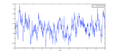
(a) The differentiated process $X_{t}$

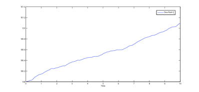
(b) The integrated process $Y_{t}$

Figure 2: the Sample Paths of $X_{t}$ and $Y_{t}$

Throughout this section, we employ Gamma kernel $K_{G(x/h+1,h)}(u)=\frac{u^{x/h}\exp(-u/h)}{h^{x/h+1}\Gamma(x/h+1)}$ and Gaussian kernel $K(x)=\frac{1}{\sqrt{2\pi}}e^{-\frac{x^{2}}{2}}.$ In general, the nonparametric estimation is sensitive to bandwidth choices, hence we select the data-driven bandwidth via the bandwidth selector $h=c\hat{S}(n\Delta_{n})^{-\frac{2}{5}}=c\hat{S}T^{-\frac{2}{5}}$ for “interior x” or $h=c\hat{S}(n\Delta_{n})^{-\frac{1}{5}}=c\hat{S}T^{-\frac{1}{5}}$ for “boundary x” similarly as Xu and Phillips [50], where $\hat{S}$ denotes the standard deviation of the data and c represents different constants for different cases, or cross-validation method in Racine [38] according to Remark 7. We will compare their mean square error (MSE) under various lengths of observation time interval $T~{}(=50,100,500)$ and sample sizes $n~{}(=500,1000,5000)$ with $\Delta_{n}=\frac{T}{n}.$ For comparison of coverage rate and length of confidence band, we will consider three design points such as the boundary point $x=0.05$ and interior point $x=0.15,0.30,$ which fall in the range of the simulated data. Meanwhile, we will also consider five fixed bandwidth $(h_{1},h_{2},h_{3},h_{4},h_{opt})=(0.01,0.02,0.03,0.05,0.0441)$ for estimation of $\mu(x)$ and $(h_{1},h_{2},h_{3},h_{4},h_{opt})=(0.01,0.02,0.04,0.05,0.0294)$ for estimation of $M(x)$ as that in Xu [49], which cover the bandwidths used in practice. In this section, the normal confidence level is assumed to be $95\%.$

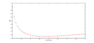
(a) Curve of $MSE(h)$ versus $C$ in $h$ with $C_{opt}=2.8$

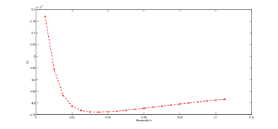
(b) Curve of $CV(h)$ versus $h$ with $h_{cv}=0.035$

Figure 3: Curve for two rules of thumb versus $h$ with $T=10,~{}n=1000$ of $\mu(x)=1-10*x$

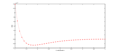
(a) Curve of $MSE(h)$ versus $C$ in $h$ with $C_{opt}=1.7$

(b) Curve of $CV(h)$ versus $h$ with $h_{cv}=0.025$

Figure 4: Curve for two rules of thumb versus $h$ with $T=10,~{}n=1000$ of $M(x)=0.1+0.1*x^{2}+2*0.036^{2}$

Firstly, we select the data-driven bandwidth by calculating MSE or $k-$block CV as a function of $h_{n}$ from a sample with $T=10$ and $n=1000$ under two rules of thumb in Remark 7 for estimation of both $\mu(x)$ and $M(x)$, which are shown in Figure 3 and 4. We can get the optimal bandwidths $h_{n}$ for theses two cases on estimating $\mu(x)$ by means of minimizing MSE or $k-$block CV, which are $h_{opt}=0.0683$ with $c_{opt}=2.8$ which coincides with that in Xu and Phillips [50] and $h_{cv}=0.035.$ Although $h_{cv}$ is smaller than $h_{opt},$ the performance of the estimator with $h_{cv}$ is a little worse than that with $h_{opt},$ which can be tested and verified in Figures 5 and 6.

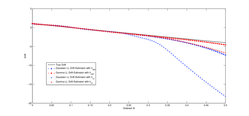
Figure 5: Local Linear Estimators for $\mu(x)=1-10*x$ based on Gaussian and Gamma kernels with $T=10,~{}n=1000,~{}h_{opt}=2.8*\hat{S}*T^{-2/5}=0.0683,~{}h_{cv}=0.035$

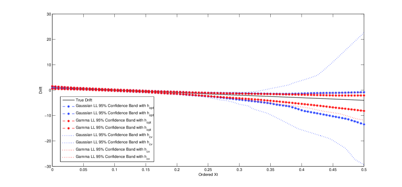
Figure 6: 95% Monte Carlo confidence intervals for $\mu(x)=1-10*x$ based on Gaussian and Gamma kernels with $T=10,~{}n=1000,~{}h_{opt}=2.8*\hat{S}*T^{-2/5}=0.0683,~{}h_{cv}=0.035$

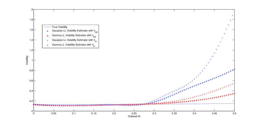
Figure 7: Local Linear Estimators for $M(x)=0.1+0.1*x^{2}+2*0.036^{2}$ based on Gaussian and Gamma kernels with $T=10,~{}n=1000,~{}h_{opt}=1.7*\hat{S}*T^{-2/5}=0.0441,~{}h_{cv}=0.025$

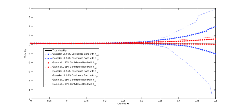
Figure 8: 95% Monte Carlo confidence intervals for $M(x)=0.1+0.1*x^{2}+2*0.036^{2}$ based on Gaussian and Gamma kernels with $T=10,~{}n=1000,~{}h_{opt}=1.7*\hat{S}*T^{-2/5}=0.0441,~{}h_{cv}=0.025$

Figures 5 and 6 represent the local linear estimator and $95\%$ Monte Carlo confidence intervals constructed with Gamma asymmetric kernels and Gaussian symmetric kernels for $\mu(x)$ from a sample with $T=10$ and $n=1000$ under two rules of thumb for $h_{n},$ which show the local linear estimator constructed with Gamma asymmetric kernels performs a little better and the $95\%$ Monte Carlo confidence intervals constructed with Gamma asymmetric kernels are shorter than that constructed with Gaussian symmetric kernels which reveals smaller variability, especially at the sparse design point. In addition, the local linear estimator constructed with $h_{n}=c*\hat{S}*T^{-2/5}$ performs a little better and the $95\%$ Monte Carlo confidence intervals constructed with $h_{n}=c*\hat{S}*T^{-2/5}$ are shorter than that constructed with $h_{cv}.$ In the subsequent numeral calculations such as MSE, coverage rate and lengths of confidence band, we will calculate the estimators with $h_{n}=c*\hat{S}*T^{-2/5}.$ Additionally, from Figure 5 we can observe that the local linear estimator constructed with Gaussian symmetric kernels exhibits a higher downward bias than that constructed with Gamma asymmetric kernels which is practically unbiased, which coincides with that in Gospodinov and Hirukawa [18].

Similar results for estimation of $M(x)$ can be observed from Figure 4, 7 and 8. Inconsistently, the optimal bandwidths $h_{n}$ on estimating $M(x)$ by means of minimizing MSE or $k-$block CV are $h_{opt}=0.0441$ with $c_{opt}=1.7$ which coincides with that in Xu and Phillips [50] and $h_{cv}=0.025.$ Compared with the optimal smoothing parameter for $\mu(x),$ it is observed that a narrower one for $M(x)$, as documented in Chapman and Pearson [6]. From Figure 7, we can observe that the local linear estimator constructed with Gaussian symmetric kernels exhibits a higher upward bias than that constructed with Gamma asymmetric kernels, which may be caused by the discretization bias similarly as the microstructure noise in empirical market.

Remark 12

As proposed in Hirukawa and Sakudo [24], the “rule of thumb” smoothing bandwidth should be under consideration for each cases such as various $T$ and $n,$ which should be determined by the specific financial data. As depicted in Figure 9, contrary to $h_{opt}$ with $c_{opt}=2.8$ for a sample with $T=10$ and $n=1000,$ the estimated parameters $c_{opt}$ in $h_{opt}$ based on a sample with $T=50$ and $n=5000$ or $T=100$ and $n=5000$ are 3 or 3.7. The $c_{opt}$ in $h_{opt}$ get larger as the time span $T$ expands larger, which may be due to the fact that $h_{opt}=c\cdot\hat{S}\cdot T^{-2/5}$ is inversely proportional to $T$ and the fact that the smaller $h_{n}$, the larger bias from Figure 3, 4 and 9. In order to effectively compare the local linear estimator constructed with Gamma asymmetric kernel with that using Gaussian symmetric kernel in terms of MSE, we should calculate the $c_{opt}$ in $h_{opt}$ for various $T$ and $n.$ Here we omit these calculations for $c_{opt}.$

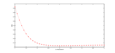
(a) $C_{opt}=3$ for $T=50,~{}n=5000$ with $h_{opt}=0.0441$ (0.0412 if $C=2.8$)

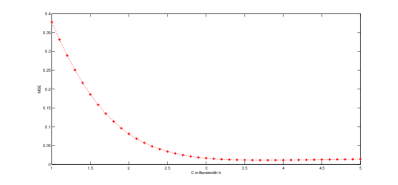
(b) $C_{opt}=3.7$ for $T=100,~{}n=5000$ with $h_{opt}=0.0435$ (0.0329 if $C=2.8$)

Figure 9: Curve for $MSE(h)$ versus $C$ in $h=C*\hat{S}*T^{-2/5}$ under $n=5000$ and various $T$ of $\mu(x)=1-10*x$

We will assess the performance of the local linear estimators constructed with Gamma asymmetric kernels and those constructed with Gaussian symmetric kernels for both drift and conditional variance functions via the Mean Square Errors (MSE)

$$MSE=\frac{1}{m}\sum_{k=0}^{m}\left\{\hat{\mu}(x_{k})-\mu(x_{k})\right\}^{2},$$ (20)

where $\hat{\mu}(x)$ is the estimator of $\mu(x)$ and $\{x_{k}\}_{1}^{m}$ are chosen uniformly to cover the range of sample path of $X_{t}.$ Table 2 gives the results on the MSE of local linear estimator constructed with Gamma asymmetric kernels (MSE-LL(Gamma)) and local linear estimator constructed with Gaussian symmetric kernels (MSE-LL(Gaussian)) for the drift function $\mu(x)$ with jump size $Z_{n}\sim\mathscr{N}(0,0.036^{2})$ over 500 replicates. Table 3 reports the results on MSE-LL(Gamma) and MSE-LL(Gaussian) for $M(x)$.

From Table 2 and 3, we can make the following remarks.

• The local linear estimator for $\mu(x)$ and $M(x)$ constructed with Gamma asymmetric kernels performs a little better than that constructed with Gaussian symmetric kernels in terms of MSE;

• For the same time interval $T$, as the sample sizes $n$ tends larger, the performances of the estimators for $\mu(x)$ or $M(x)$ are improved due to the fact that more information for estimation procedure is sampled as $\Delta_{n}\rightarrow 0;$

• For the same sample sizes $n$, as the time interval $T$ expands larger, the performance of the estimator for $\mu(x)$ is improved due to the fact that the more information about drift coefficient is obtained as the time span get larger, however, the performance of the estimator for $M(x)$ gets worse, especially when $T=100$, due to the fact that more jumps happens in larger time interval $T$ in steps 3 of Algorithm 1;

• To some extent, the previous remark confirms that the drift and conditional variance functions cannot be identified in a fixed time span, which corresponds to the results of Theorem 2.

Table 2: Simulation results on MSE-LL(Gaussian), MSE-LL(Gamma) for three lengths of time interval (T) and three sample sizes for $\mu(x)=1-10x$ with arrival intensity $\lambda\cdot T=20$, jump size $Z_{n}\sim\mathscr{N}(0,0.036^{2})$ and $h_{opt}$ over 500 replicates.

T		$n=500$	$n=1000$	$n=5000$
10	MSE-LL(Gaussian)	0.5818	0.5253	0.0833
	MSE-LL(Gamma)	0.3010	0.1511	0.0424
50	MSE-LL(Gaussian)	0.5075	0.7499	0.1596
	MSE-LL(Gamma)	0.1373	0.0874	0.0154
100	MSE-LL(Gaussian)	0.0364	0.0351	0.0078
	MSE-LL(Gamma)	0.0187	0.0093	0.0022

Table 3: Simulation results on MSE-LL(Gaussian), MSE-LL(Gamma) for three lengths of time interval (T) and three sample sizes for $M(x)=0.1+0.1*x^{2}+\lambda*0.036^{2}$ with arrival intensity $\lambda\cdot T=20$, jump size $Z_{n}\sim\mathscr{N}(0,0.036^{2})$ and $h_{opt}$ over 500 replicates.

T		$n=500$	$n=1000$	$n=5000$
10	MSE-LL(Gaussian)	0.1268	0.0337	0.0019
	MSE-LL(Gamma)	0.0084	0.0047	$3.7014\times 10^{-4}$
50	MSE-LL(Gaussian)	0.1153	0.0169	0.0079
	MSE-LL(Gamma)	0.0079	$5.7058\times 10^{-4}$	$3.1990\times 10^{-4}$
100	MSE-LL(Gaussian)	10.7405	0.0649	0.0089
	MSE-LL(Gamma)	27.9961	0.0025	0.0011

Figure 10 and 11 give the QQ plots for the local linear estimators of the drift function $\mu(x)$ and conditional variance function $M(x)$ constructed with Gamma asymmetric kernels and those constructed with Gaussian symmetric kernels with $T=50$ and $\Delta_{n}=0.01$. This reveals the normality of the local linear estimators of the drift function $\mu(x)$ and conditional variance function $M(x)$ constructed with Gamma asymmetric kernels, which confirms the results in Theorems 2.

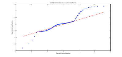
(a) QQ plot using Gaussian kernels

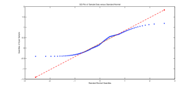
(b) QQ plot using Gamma kernels

Figure 10: QQ plot of local linear estimators for $\mu(x)=1-10*x$ using Gaussian and Gamma kernels with $T=50,~{}n=5000,~{}h_{opt}=3*\hat{S}*T^{-2/5}=0.0441$

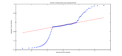
(a) QQ plot using Gaussian kernels

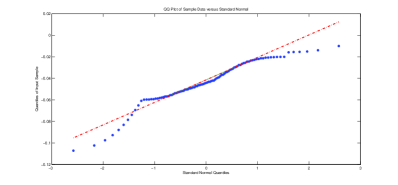
(b) QQ plot using Gamma kernels

Figure 11: QQ plot of local linear estimators for $M(x)=0.1+0.1*x^{2}+20/50*0.036^{2}$ using Gaussian and Gamma kernels with $T=50,~{}n=5000,~{}h_{opt}=1.9*\hat{S}*T^{-2/5}=0.0294$

The computational results about comparison of coverage rate and length of confidence band for drift $\mu(x)$ are summarized in Table 4 - 6 and conditional variance $M(x)$ in Table 9 for various intensity and amplitude of jumps with $T=50,~{}n=5000.$ The confidence intervals are constructed as those in Remark 9. For “boundary $x=0.05$” or “interior $x=0.15$”, we also calculate the adjusted lengths of confidence band for $\mu(x)$ which was argued for in Xu [49]. The adjusted lengths of the calibrated confidence intervals constructed with the actual critical values are presented in Table 7 - 8. The actual critical values marked as $2.5\%$ or $97.5\%$ quantile in Table 7 - 8 are adapt to actual simulation data and no longer 1.96 as that in the standard normal distribution table for asymptotic normality such that the coverage rates are adjusted to $95\%.$ Note that the ratio in tables denotes the ratio of the length of confidence band constructed with Gaussian symmetric kernel (CB-GSK) to that constructed with Gamma asymmetric kernel (CB-GAK). From these six tables, we can obtain the following findings.

• From Table 4, for the drift function, according to the coverage rates in percent, CB-GSK or CB-GAK are more under-covered as $h_{n}$ expands larger, especially at the “boundary $x=0.05$” or the sparse “interior $x=0.30$”. When $x=0.15,$ CB-GSK or CB-GAK has favorable lengths for the bandwidths $h_{n}.$ The reasons behind the phenomenon may be the following three aspects. Firstly, estimations for asymptotic variance at design points $x=0.05,0.30$ based on the formula in Theorem 2 are more slightly below the sample variance of the randomly generated data, which may be the main reason. Secondly, the process visits the design points $x=0.05,0.30$ less frequently such that there are relatively less sample points near their neighborhood to estimate the unknown quantity. The first two reasons coincide with those observed in Xu [49]. Thirdly, as shown in Remark 9, the bias in the normal confidence interval is estimated by taking the second derivative of the local linear estimators,which may give rise to estimation bias. Also, one can see that at the “boundary point x = 0.05”, the coverage rate with GSK is a little better than that with GAK, which may be due to the facts: CB-GSK can allocate weight to the observations less than zero while CB-GAK can’t.

• From Table 4 - 6, the absolute mean of bias and variance for estimator constructed with Gamma asymmetric kernels are less than that constructed with Gaussian symmetric kernels, which indicates that compared with that constructed with Gaussian symmetric kernels, estimator constructed with Gamma asymmetric kernels is practically unbiased and exhibits smaller variability for either the boundary point or the spare design point. This coincides with the discussion of coverage rate in Remark 10, as documented in Gospodinov and Hirukawa [18].

• From Table 4 - 6, it is observed that for the same design point $x$, the ratio is more than 1 under the condition that the confidence rate is approximate, that is CB-GSK is longer than CB-GAK. Meanwhile, CB-GSK or CB-GAK expands larger and the ratio becomes bigger as $x$ increases, especially at the sparse design point $x=0.30.$ One can also find that the ratio becomes smaller as the smoothing parameter $h_{n}$ gets larger, especially at the boundary design point $x=0.05,$ which coincides with the theoretical results discussed in Remark 10. Note that the smaller the smoothing parameter $h_{n}$, the larger the bias. Hence the choice of smoothing parameter $h_{n}$ is not recommended to be too large or too small and should depend on the need for higher coverage rate or lower bias. As the intensity and amplitude of jump increases, CB-GSK or CB-GAK expands larger to improve coverage rate since it needs more information to cover more and larger jump similarly as that mentioned in Bandi and Nguyen [2].

• Here we discuss the adjusted lengths of confidence intervals constructed with various kernels since the two findings above indicate that the reasonably correct coverage rate depends on the choice of smoothing bandwidth $h_{n}$ and the consistently estimated variance. From Table 7 for “boundary $x=0.05$”, after confidence rates are adjusted to $95\%,$ the adjusted lengths of confidence intervals constructed with Gamma asymmetric kernel (ACI-GAK) are shorter than that constructed with Gaussian symmetric kernel (ACI-GSK) with the smoothing parameter $h_{n}=0.01,0.02,0.03,$ however, ACI-GAK are longer than ACI-GSK with $h_{n}=0.0441,0.05,$ which coincides with the conclusion in Remark 10 that the closer to the boundary point or the larger bandwidth for fixed “boundary $x$”, the shorter the length of confidence interval based on Gaussian symmetric kernel. In addition, the lengths of ACI-GAK are more robust as the smoothing parameter $h_{n}$ changes. One can also observe that the absolute critical values for ACI-GAK or ACI-GSK are almost larger than 1.96 for adjusted lengths, which provides a reference point for empirical analysis when constructing the confidence intervals. In Table 8, for “interior $x=0.15$”, ACI-GAK are shorter than ACI-GSK with all $h_{n}$ mentioned and the absolute critical values for ACI-GAK or ACI-GSK are almost larger than 1.96 for adjusted lengths. Constructed with the Gamma asymmetric kernel, the adjustment for $\mu(0.15)$ is milder relative to $\mu(0.05)$ for any given bandwidth or intensity and amplitude of jumps, which is because that there are plenty of sample points used to estimate $\mu(x)$ near the design point $x=0.15$ such that the coverage rate for $\mu(0.15)$ is close to $95\%$ in Table 4 - 6.

• For simplicity, similar observations for the conditional variance $M(x)$ only at “interior $x=0.15$” are shown in Table 9. Similarly as the drift function, the ratio is more than 1 under the condition that the confidence rate is approximate, that is CB-GAK is shorter than CB-GSK. Meanwhile, the ratio becomes smaller as the smoothing parameter $h_{n}$ gets larger and the intensity and amplitude of jump increases. Compared with the mean of bias of the estimator for $\mu(0.15)$ in Table 4 - 6, the mean of bias for $M(0.15)$ constructed with Gamma asymmetric kernels is larger than that constructed with Gaussian symmetric kernels. As mentioned in Theorem 2 and Remark 9, for the estimators constructed with Gamma asymmetric kernels at “interior $x=0.15$”, the bias for ${\mu}(x)$ in model (17) is $h_{n}B_{\hat{\mu}_{n}(x)}=h_{n}\frac{x}{2}\mu^{{}^{\prime\prime}}(x)\equiv 0,$ which is equal to the bias of the estimator constructed with Gaussian symmetric kernels, that is also $0.$ However, the bias for ${M}(x)$ is $h_{n}B_{\hat{M}_{n}(x)}=h_{n}\frac{x}{2}M^{{}^{\prime\prime}}(x)=h_{n}\cdot 0.1\cdot x=O(h_{n})$ which is far greater than the bias of the estimator constructed with Gaussian symmetric kernels, that is $O(h_{n}^{2}).$ Furthermore, this observation does not contradict with the result on MSE considered previously because the variance of the estimator for $M(0.15)$ constructed with Gamma asymmetric kernels is less than that constructed with Gaussian symmetric kernels and the variance dominates the MSE.

Table 4: Estimation for $\mu(x)$ with arrival intensity $\lambda\cdot T=20$, jump size $Z_{n}\sim\mathscr{N}(0,0.036^{2})$ over 500 replicates.

Bandwidth	Coverage Rate		Mean of Bias		Variance		Estimation for Variance				Length of Confidence Band
	Sym	Asym	Sym	Asym	Sym	Asym	Sym	Std	Asym	Std	Sym	Asym	Ratio
x = 0.05
$h_{1}=0.01$	94.6	92.4	0.0045	0.0028	0.0144	0.0067	0.0136	0.0011	0.0057	0.0004	0.457	0.2954	1.5471
$h_{2}=0.02$	94.6	89.6	0.0032	0.0011	0.007	0.0055	0.0069	0.0005	0.0039	0.0002	0.3262	0.2456	1.3282
$h_{3}=0.03$	94.2	88	0.0022	0.0003	0.0049	0.005	0.0048	0.0003	0.0032	0.0002	0.2701	0.2217	1.2183
$h_{4}=0.05$	93.6	84	0.0018	-0.0002	0.0037	0.0046	0.0031	0.0002	0.0025	0.0001	0.2178	0.1976	1.1022
$h_{opt}=0.0441$	93.8	84.6	0.0018	-0.0001	0.0038	0.0047	0.0033	0.0002	0.0026	0.0001	0.2253	0.2012	1.1198
x = 0.15
$h_{1}=0.01$	94.4	94.2	-0.0038	-0.004	0.0139	0.0042	0.0142	0.0013	0.0042	0.0003	0.4659	0.2538	1.8357
$h_{2}=0.02$	95.6	94	-0.005	-0.0036	0.0072	0.0035	0.0072	0.0005	0.0033	0.0002	0.332	0.225	1.4756
$h_{3}=0.03$	93.2	94	-0.0045	-0.0035	0.0051	0.0032	0.0049	0.0003	0.0029	0.0001	0.2745	0.212	1.2948
$h_{4}=0.05$	93.6	93.4	-0.0034	-0.0033	0.0036	0.003	0.0032	0.0002	0.0026	0.0001	0.2208	0.1993	1.1079
$h_{opt}=0.0441$	93.6	93.2	-0.0036	-0.0033	0.0038	0.003	0.0034	0.0002	0.0026	0.0001	0.2285	0.2012	1.1357
x = 0.30
$h_{1}=0.01$	94.4	95	-0.1856	-0.0913	0.863	0.14	0.7196	0.5996	0.125	0.0538	3.1606	1.3587	2.3262
$h_{2}=0.02$	89.6	89.2	-0.1702	-0.0581	0.4349	0.0853	0.2866	0.1626	0.058	0.0196	2.0382	0.9319	2.1871
$h_{3}=0.03$	86.2	87.2	-0.138	-0.0421	0.2695	0.0644	0.1443	0.0607	0.0369	0.0109	1.4629	0.7458	1.9615
$h_{4}=0.05$	76.6	81	-0.0806	-0.0277	0.125	0.0474	0.0477	0.0119	0.0214	0.0052	0.8498	0.5691	1.4932
$h_{opt}=0.0441$	79.6	81.8	-0.0929	-0.0299	0.1486	0.05	0.0596	0.0196	0.0235	0.0064	0.946	0.5962	1.5867

Table 5: Estimation for $\mu(x)$ with arrival intensity $\lambda\cdot T=50$, jump size $Z_{n}\sim\mathscr{N}(0,0.036^{2})$ over 500 replicates.

Bandwidth	Coverage Rate		Mean of Bias		Variance		Estimation for Variance				Length of Confidence Band
	Sym	Asym	Sym	Asym	Sym	Asym	Sym	Std	Asym	Std	Sym	Asym	Ratio
x = 0.05
$h_{1}=0.01$	95.2	92	0.0027	0.0005	0.0138	0.0069	0.0137	0.0013	0.0057	0.0004	0.4586	0.2965	1.5467
$h_{2}=0.02$	95	90	0.0019	0.0006	0.0068	0.0056	0.007	0.0005	0.004	0.0002	0.3271	0.2465	1.3270
$h_{3}=0.03$	94.6	88.8	0.0018	0.0007	0.0049	0.0051	0.0048	0.0003	0.0032	0.0002	0.2709	0.2226	1.2170
$h_{4}=0.05$	92.6	86.4	0.002	0.0009	0.0036	0.0047	0.0031	0.0002	0.0026	0.0001	0.2185	0.1984	1.1013
$h_{opt}=0.0441$	93.8	86.8	0.0019	0.0009	0.0038	0.0047	0.0033	0.0002	0.0027	0.0001	0.2259	0.202	1.1183
x = 0.15
$h_{1}=0.01$	95.4	94.2	-0.0029	-0.0091	0.0134	0.0045	0.0143	0.0013	0.0043	0.0003	0.469	0.2556	1.8349
$h_{2}=0.02$	95.8	93.4	-0.0071	-0.0094	0.007	0.0039	0.0073	0.0005	0.0033	0.0002	0.3343	0.2265	1.4759
$h_{3}=0.03$	94.4	92.6	-0.0085	-0.0095	0.0052	0.0036	0.005	0.0003	0.003	0.0001	0.2764	0.2135	1.2946
$h_{4}=0.05$	92.2	91.2	-0.009	-0.0096	0.004	0.0034	0.0032	0.0002	0.0026	0.0001	0.2222	0.2006	1.1077
$h_{opt}=0.0441$	92.6	91.2	-0.009	-0.0096	0.0042	0.0035	0.0034	0.0002	0.0027	0.0001	0.2299	0.2025	1.1353
x = 0.30
$h_{1}=0.01$	93.4	94	-0.1792	-0.0942	0.8427	0.1411	0.7276	0.6509	0.1244	0.0672	3.1579	1.3501	2.3390
$h_{2}=0.02$	92.2	87.8	-0.1605	-0.06	0.4074	0.0893	0.2826	0.1555	0.0576	0.0217	2.0249	0.9271	2.1841
$h_{3}=0.03$	89.2	83	-0.1365	-0.0431	0.257	0.0679	0.1429	0.058	0.0367	0.0115	1.4564	0.7426	1.9612
$h_{4}=0.05$	76	77.8	-0.083	-0.0275	0.1272	0.0495	0.0476	0.0114	0.0213	0.0054	0.8491	0.5674	1.4965
$h_{opt}=0.0441$	79.2	78.6	-0.0945	-0.0298	0.1483	0.0522	0.0588	0.0187	0.0233	0.0066	0.9396	0.5929	1.5848

Table 6: Estimation for $\mu(x)$ with arrival intensity $\lambda\cdot T=20$, jump size $Z_{n}\sim\mathscr{N}(0,0.1^{2})$ over 500 replicates.

Bandwidth	Coverage Rate		Mean of Bias		Variance		Estimation for Variance				Length of Confidence Band
	Sym	Asym	Sym	Asym	Sym	Asym	Sym	Std	Asym	Std	Sym	Asym	Ratio
x = 0.05
$h_{1}=0.01$	94.2	93.6	-0.0114	-0.0074	0.0142	0.0071	0.0142	0.0014	0.0059	0.0004	0.4671	0.3019	1.5472
$h_{2}=0.02$	95.6	88.6	-0.0068	-0.0056	0.0075	0.006	0.0072	0.0006	0.0041	0.0003	0.3333	0.2509	1.3284
$h_{3}=0.03$	94	86	-0.0045	-0.0046	0.0055	0.0055	0.0050	0.0003	0.0033	0.0002	0.2758	0.2264	1.2182
$h_{4}=0.05$	91.2	83.2	-0.0019	-0.0035	0.004	0.0051	0.0032	0.0002	0.0026	0.0001	0.2222	0.2017	1.1016
$h_{opt}=0.0441$	91.2	83	-0.0022	-0.0036	0.0042	0.0051	0.0034	0.0002	0.0027	0.0001	0.2283	0.2046	1.1158
x = 0.15
$h_{1}=0.01$	95	94.8	-0.0073	-0.005	0.0142	0.0043	0.0147	0.0015	0.0044	0.0003	0.4753	0.2587	1.8373
$h_{2}=0.02$	94.4	94	-0.0062	-0.0045	0.0073	0.0035	0.0075	0.0006	0.0034	0.0002	0.3387	0.2292	1.4777
$h_{3}=0.03$	93.8	94	-0.0055	-0.0043	0.0051	0.0033	0.0051	0.0003	0.003	0.0002	0.2799	0.2159	1.2964
$h_{4}=0.05$	93.4	93.2	-0.0043	-0.004	0.0037	0.0031	0.0033	0.0002	0.0027	0.0001	0.225	0.203	1.1084
$h_{opt}=0.0441$	93.4	93.2	-0.0045	-0.0041	0.0038	0.0031	0.0035	0.0002	0.0027	0.0001	0.2314	0.2045	1.1315
x = 0.30
$h_{1}=0.01$	95	94.4	-0.1758	-0.0828	0.764	0.1299	0.6683	0.5664	0.1073	0.0468	3.0489	1.2594	2.4209
$h_{2}=0.02$	90.8	88.4	-0.1562	-0.0542	0.3728	0.0807	0.2704	0.1552	0.051	0.0176	1.9791	0.8742	2.2639
$h_{3}=0.03$	87.6	84.6	-0.1256	-0.0402	0.2393	0.0616	0.1392	0.0619	0.033	0.0099	1.4352	0.7045	2.0372
$h_{4}=0.05$	80.8	79.8	-0.0734	-0.0275	0.1176	0.0461	0.0475	0.0131	0.0194	0.0049	0.8471	0.5425	1.5615
$h_{opt}=0.0441$	82.6	79.8	-0.0823	-0.0291	0.1355	0.0481	0.0569	0.0199	0.021	0.0058	0.9234	0.5628	1.6407

Table 7: Adjusted length of confidence band for $\mu(0.05)$ over 500 replicates.

Bandwidth	Coverage Rate		Sym Quantile		Asym Quantile		Length of Confidence Band
	Sym	Asym	2.50%	97.50%	2.50%	97.50%	Sym	Asym	Ratio
Arrival intensity $\lambda\cdot T=20$, Jump size $Z_{n}\sim\mathscr{N}(0,0.036^{2})$
$h_{1}=0.01$	95.2	95.2	-2.1465	1.8766	-2.2883	2.2854	0.4703	0.3453	1.362
$h_{2}=0.02$	95.2	95.2	-2.0760	2.0444	-2.3716	2.4169	0.3435	0.3002	1.1442
$h_{3}=0.03$	95.2	95.2	-2.1586	2.1179	-2.5243	2.5791	0.295	0.2888	1.0215
$h_{4}=0.05$	95.2	95.2	-2.1865	2.2459	-2.7060	2.7412	0.2464	0.2746	0.8973
$h_{opt}=0.0441$	95.2	95	-2.1899	2.1468	-2.7222	2.6919	0.2493	0.278	0.8968
	mean		-2.1515	2.0863	-2.5225	2.5429	0.3209	0.2974	1.0791
Arrival intensity $\lambda\cdot T=50$, Jump size $Z_{n}\sim\mathscr{N}(0,0.036^{2})$
$h_{1}=0.01$	95.2	95.2	-1.9490	2.0748	-2.2026	2.2388	0.4721	0.3368	1.4017
$h_{2}=0.02$	95.2	95.2	-2.0882	2.074	-2.4857	2.5502	0.3484	0.3173	1.098
$h_{3}=0.03$	95.2	95.2	-2.0592	2.1506	-2.6234	2.5998	0.2917	0.2883	1.0118
$h_{4}=0.05$	95.2	95.2	-2.3158	2.0811	-2.7272	2.7163	0.2455	0.2758	0.8901
$h_{opt}=0.0441$	95.2	94.8	-2.2977	2.0508	-2.7281	2.6843	0.2508	0.279	0.8989
	mean		-2.142	2.0863	-2.5534	2.5579	0.3217	0.2994	1.0743
Arrival intensity $\lambda\cdot T=20$, Jump size $Z_{n}\sim\mathscr{N}(0,0.1^{2})$
$h_{1}=0.01$	95.2	95.2	-2.0544	1.8202	-2.1361	2.1092	0.4599	0.3258	1.4116
$h_{2}=0.02$	95.2	95.2	-1.8318	1.8576	-2.4108	2.2472	0.3124	0.2973	1.0508
$h_{3}=0.03$	95.2	95.2	-2.0650	1.9779	-2.5856	2.4245	0.2834	0.2811	1.0081
$h_{4}=0.05$	95.2	95.2	-2.1245	2.086	-2.8735	2.5503	0.2381	0.2786	0.8546
$h_{opt}=0.0441$	95.2	95.2	-2.1531	2.0896	-2.8347	2.5017	0.2468	0.2783	0.8868
	mean		-2.0458	1.9663	-2.5681	2.3666	0.3081	0.2922	1.0544

Table 8: Adjusted length of confidence band for $\mu(0.15)$ over 500 replicates.

Bandwidth	Coverage Rate		Sym Quantile		Asym Quantile		Length of Confidence Band
	Sym	Asym	2.50%	97.50%	2.50%	97.50%	Sym	Asym	Ratio
Arrival intensity $\lambda\cdot T=20$, Jump size $Z_{n}\sim\mathscr{N}(0,0.036^{2})$
$h_{1}=0.01$	95.2	95.2	-2.0012	2.0126	-1.9856	2.1802	0.4761	0.2695	1.7666
$h_{2}=0.02$	95.2	95.2	-1.9823	2.0154	-1.9710	2.1613	0.3381	0.237	1.4266
$h_{3}=0.03$	95.2	95.2	-2.0890	2.1366	-1.9350	2.3658	0.2956	0.2325	1.2714
$h_{4}=0.05$	95.2	95.2	-2.0606	2.2294	-1.9769	2.3788	0.2415	0.2214	1.0908
$h_{opt}=0.0441$	95.2	94.8	-2.0697	2.2194	-1.9547	2.3841	0.2498	0.2226	1.1222
	mean		-2.0406	2.1227	-1.9646	2.294	0.3202	0.2366	1.3534
Arrival intensity $\lambda\cdot T=50$, Jump size $Z_{n}\sim\mathscr{N}(0,0.036^{2})$
$h_{1}=0.01$	95.2	95.2	-2.1808	2.0987	-1.9418	2.1174	0.51	0.2638	1.9333
$h_{2}=0.02$	95.2	95.2	-1.9529	2.3189	-2.1120	2.0546	0.363	0.2401	1.5119
$h_{3}=0.03$	95.2	95.2	-1.9840	2.3023	-2.1067	2.0558	0.3013	0.2261	1.3326
$h_{4}=0.05$	95.2	95.2	-2.1573	2.1565	-2.2084	2.101	0.244	0.2201	1.1086
$h_{opt}=0.0441$	95.2	95	-2.1034	2.1938	-2.2020	2.1022	0.2511	0.2218	1.1321
	mean		-2.0757	2.214	-2.1142	2.0862	0.3339	0.2344	1.4245
Arrival intensity $\lambda\cdot T=20$, Jump size $Z_{n}\sim\mathscr{N}(0,0.1^{2})$
$h_{1}=0.01$	95.2	95.2	-2.0582	2.0251	-2.0616	2.2115	0.494	0.2821	1.7512
$h_{2}=0.02$	95.2	95.2	-2.0097	2.1434	-2.1454	2.2018	0.3585	0.2544	1.4092
$h_{3}=0.03$	95.2	95.2	-2.0967	2.1874	-2.1593	2.2739	0.3059	0.2445	1.2511
$h_{4}=0.05$	95.2	95.2	-2.1265	2.2835	-2.1661	2.3895	0.2534	0.2363	1.0724
$h_{opt}=0.0441$	95.2	95.2	-2.0901	2.3064	-2.1598	2.3709	0.2596	0.2367	1.0967
	mean		-2.0762	2.1892	-2.1384	2.2895	0.3343	0.2508	1.3329

Table 9: Estimation for $M(0.15)$ over 500 replicates.

Bandwidth	Coverage Rate		Mean of Bias		Variance ($\times 10^{-4}$)		Estimation for Variance ($\times 10^{-4}$)				Length of Confidence Band
	Sym	Asym	Sym	Asym	Sym	Asym	Sym	Std	Asym	Std	Sym	Asym	Ratio
Arrival intensity $\lambda\cdot T=20$, Jump size $Z_{n}\sim\mathscr{N}(0,0.036^{2})$
$h_{1}=0.01$	94.8	94.8	0.004	0.0049	0.3221	0.0991	0.4581	0.0679	0.1369	0.0125	0.0265	0.0145	1.8276
$h_{2}=0.02$	92	90.4	0.0043	0.0053	0.1669	0.0821	0.233	0.0268	0.108	0.0087	0.0189	0.0129	1.4651
$h_{3}=0.04$	76.4	79.2	0.0048	0.0058	0.0985	0.0731	0.1242	0.0108	0.0895	0.0065	0.0138	0.0117	1.1795
$h_{4}=0.05$	68.6	68.6	0.0051	0.0059	0.0867	0.0714	0.1037	0.0082	0.0852	0.006	0.0126	0.0114	1.1053
$h_{opt}=0.0294$	85	86.2	0.0045	0.0056	0.1237	0.0766	0.1647	0.0162	0.097	0.0073	0.0159	0.0122	1.3033
Arrival intensity $\lambda\cdot T=50$, Jump size $Z_{n}\sim\mathscr{N}(0,0.036^{2})$
$h_{1}=0.01$	94.6	93	0.0034	0.0045	0.329	0.1114	0.4626	0.0692	0.1392	0.0132	0.0266	0.0146	1.8219
$h_{2}=0.02$	91	89.8	0.0038	0.005	0.1807	0.0911	0.2361	0.0276	0.11	0.0094	0.019	0.013	1.4615
$h_{3}=0.04$	79.8	82.6	0.0045	0.0056	0.109	0.0803	0.1263	0.0116	0.0913	0.0071	0.0139	0.0118	1.1780
$h_{4}=0.05$	72.2	72.6	0.0048	0.0057	0.096	0.0784	0.1056	0.0089	0.087	0.0066	0.0127	0.0116	1.0948
$h_{opt}=0.0294$	87	85.4	0.0041	0.0053	0.1356	0.0843	0.1662	0.0168	0.0987	0.0079	0.016	0.0123	1.3008
Arrival intensity $\lambda\cdot T=20$, Jump size $Z_{n}\sim\mathscr{N}(0,0.1^{2})$
$h_{1}=0.01$	95	93.8	0.0038	0.0046	0.5407	0.1829	0.6642	0.3883	0.1961	0.0698	0.0311	0.0171	1.8187
$h_{2}=0.02$	93	91.2	0.004	0.0052	0.3149	0.1456	0.3372	0.1509	0.154	0.0487	0.0224	0.0152	1.4737
$h_{3}=0.04$	85.2	85.2	0.0046	0.0057	0.179	0.1276	0.1778	0.0614	0.1272	0.0371	0.0163	0.0139	1.1727
$h_{4}=0.05$	78.2	79.2	0.0049	0.0058	0.1544	0.1246	0.1481	0.0471	0.1211	0.0347	0.0149	0.0135	1.1037
$h_{opt}=0.0294$	88.6	87.8	0.0043	0.0055	0.2285	0.1339	0.2323	0.0889	0.1373	0.041	0.0186	0.0144	1.2917

5 Empirical Analysis

In this section, we apply the second-order jump-diffusion to model the return of stock index in Shanghai Stock Exchange between July 2014 and Dec 2014 from China under five-minute high frequency data, and then apply the local linear estimators to estimate the unknown coefficients in model (3) based on Gamma asymmetric kernels and Gaussian symmetric kernels. The real-world financial market data set analyzed consists of 6048 observations.

We assume that

$$\left\{\begin{array}[]{ll}d\log Y_{t}=X_{t}dt,\\ dX_{t}=\mu(X_{t-})dt+\sigma(X_{t-})dW_{t}+\int_{\mathscr{E}}c(X_{t-},z)r(\omega,dt,dz),\end{array}\right.$$ (21)

where $\log Y_{t}$ is the log integrated process for stock index and $X_{t}$ is the latent process for the log-returns. According to (6), we can get the proxy of the latent process

$$\widetilde{X}_{i\Delta_{n}}=\frac{\log Y_{i\Delta_{n}}-\log Y_{(i-1)\Delta_{n}}}{\Delta_{n}}.$$ (22)

The plots of the stock index and its proxy (22) from China, i.e. Shanghai Composite Index in high frequency data are shown in Figure 12.

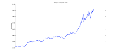
(a) Shanghai Composite Index (2014)

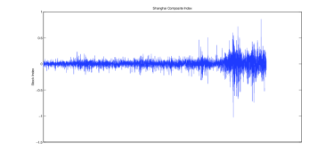
(b) Proxy of Shanghai Composite Index (2014)

Figure 12: Time Series and Proxy of Shanghai Composite Index (2014) from July 01, 2014 to Dec 31, 2014

First, we test the existence of jumps for the proxy $X_{t}$ through the test statistic proposed in Barndorff-Nielsen and Shephard [3] (denoted by BS Statistic). For five-minute high frequency data, the value of BS Statistic is -3.9955, which exceeds [-1.96, 1.96], so there exists jumps in high frequency data at the 5% significance level, which confirms the validity of model (3) not model (2) for the return of stock index by the second-order process. Based on the Augmented Dickey-Fuller test statistic, we can easily get that the null hypothesis of non-stationarity is accepted at the 5% significance level for the stock index $Y_{t}$, but is rejected for the proxy of $X_{t}$, which confirms the assumption of stationary by differencing.

Here we use two alternative smoothing parameters $h_{cv}$ which is selected by the $k-$block cross-validation method, and $h_{T}=c\cdot\hat{S}\cdot T^{-\frac{2}{5}}$ with $c=4$ for drift and $c=2$ for volatility (chosen only for illustration). Figure 13 depicts the curves of CV($h_{cv}$) versus $h_{cv}$ for Shanghai Composite Index showing that CV($h_{cv}$) is minimized at $h_{cv}=0.095$ for drift estimator, $h_{cv}=0.040$ for volatility estimator, respectively.

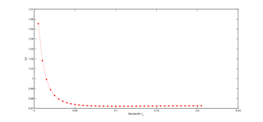
(a) $CV(h_{n})$ for drift estimator

(b) $CV(h_{n})$ for volatility estimator

Figure 13: Curve of $CV(h_{n})$ versus $h_{n}$ for Shanghai Composite Index (2014)

Then, we will employ the local linear estimators based on Gamma asymmetric kernels (11) and (12) to estimate the unknown coefficients under (22) and $\Delta_{n}=\frac{1}{48}$ for five-minute data (t = 1 meaning one day) with various bandwidth such as $h_{cv}$ and $h_{T}.$ The estimation curves for unknown qualities in five-minute high frequency data are displayed in Figure 14.

It is observed that the linear shape with negative coefficient for drift estimator in FIG 14 (a) & (b) for various bandwidths which indicates that the higher log-return increments correspond to the lower drift in the latent process (this fact coincides with the economic phenomenon of mean reversion), which reveals a negative correlation. It is also shown the quadratic form with positive coefficient for volatility estimator with a minimum at 0.3 in FIG 14 (c) & (d) which reveals that the higher absolute value of log-return increments correspond to the higher volatility in the latent process (this fact coincides with the economic phenomenon of volatility smile). These findings are consistent with those in Nicolau [34].

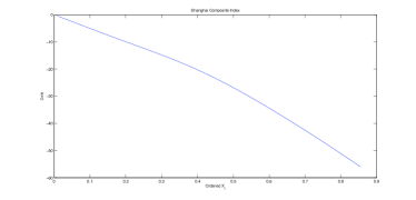
(a) Drift estimator with $h_{cv}$

(b) Drift estimator with $h_{T}$

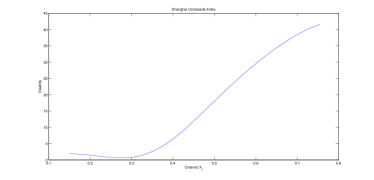
(c) Volatility estimator with $h_{cv}$

(d) Volatility estimator with $h_{T}$

Figure 14: Local linear estimators of the drift and volatility coefficients for Shanghai Composite Index (2014) based on Gamma kernels using various bandwidths

Finally, we will construct 95% normal confidence intervals for the unknown coefficients based on Gamma asymmetric kernels and Gaussian symmetric kernels under (22) and $\Delta_{n}=\frac{1}{48}$ for five-minute data (t = 1 meaning one day) with various bandwidth such as $h_{cv}$ and $h_{T}.$ The 95% normal confidence bands for the drift and volatility functions are demonstrated in Figure 15. All the quantities are computed at 120 equally spaced nonnegative ordered $\widetilde{X}_{i\Delta_{n}}$ from 0.01 to 0.601. For a more intuitive comparison of the lengths of normal confidence intervals of the drift and volatility coefficients based on Gaussian kernels and Gamma kernels for Shanghai Composite Index (2014) using various bandwidths, here the ratios of the length of confidence band constructed with Gaussian symmetric kernel (CB-GSK) to that constructed with Gamma asymmetric kernel (CB-GAK) are shown in Figure 16. Note that the blue dotted lines in Figure 16 represent the ratio value of one.

From Figures 15 and 16, we can observe the following findings.

• As for the quantities close to zero, the ratios are less than one, which coincides with the discussion in Remark 10 that the closer to the boundary point or the larger bandwidth for fixed “boundary $x$”, the shorter the length of confidence interval based on Gaussian symmetric kernel.

• As the points increase, especially at the sparse points, CB-GSK tends to be longer than CB-GAK and the ratios gradually become larger and greater than 1, which effectively verifies the efficiency gains and resistance to sparse points of local linear smoothing using Gamma asymmetric kernel through the real high frequency financial data.

• Note that some values for the ratios in Figure 16 are zero, which is due to the fact that the local linear estimators based on Gaussian symmetric kernel for conditional variance and conditional fourth moment are negative. Fortunately, the local linear estimators based on Gamma asymmetric kernel for conditional variance and conditional fourth moment are positive.

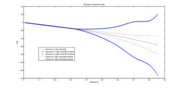
(a) Drift confidence band with $h_{cv}$

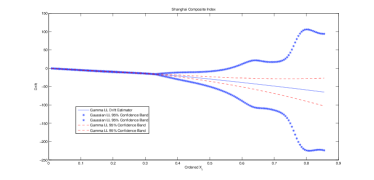
(b) Drift confidence band with $h_{T}$

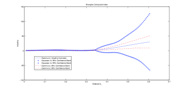
(c) Volatility confidence band with $h_{cv}$

(d) Volatility confidence band with $h_{T}$

Figure 15: 95% normal confidence intervals of the drift and volatility coefficients for Shanghai Composite Index (2014) based on Gamma kernels and Gaussian kernels using various bandwidths

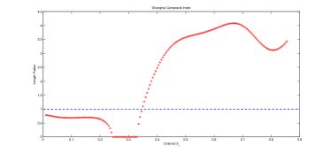
(a) Length Ratios for Drift with $h_{cv}$

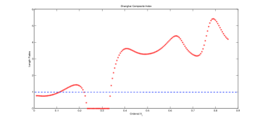
(b) Length Ratios for Drift with $h_{T}$

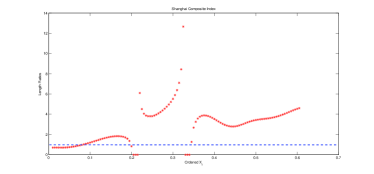
(c) Length Ratios for Volatility with $h_{cv}$

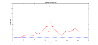
(d) Length Ratios for Volatility with $h_{T}$

Figure 16: The ratios between the lengths of normal confidence intervals of the drift and volatility coefficients based on Gaussian kernels and Gamma kernels for Shanghai Composite Index (2014) using various bandwidths

6 Conclusion

In this paper, the local linear estimators based on Gamma asymmetric kernels for the unknown drift and conditional variance in second-order jump-diffusion model. Besides the standard properties of the local linear estimation constructed with Gaussian symmetric kernels such as simple bias representation and boundary bias correction, the local linear smoothing using Gamma asymmetric kernels possesses some extra advantages such as variable bandwidth, variance reduction and resistance to sparse design, which is validated through finite sample simulation study. Theoretically, under appropriate regularity conditions, we prove that the estimators constructed with Gamma asymmetric kernels possess the consistency and asymptotic normality for large sample and verify the advantages such as bias reduction, robustness and shorter length of confidence band through simulation experiments for finite sample.

Empirically, the estimators are illustrated through stock index in China under five-minute high-frequency data and possess some advantages mentioned above. This means the second-order jump-diffusion model may be an alternative model to describe the dynamic of some financial data, especially to explain integrated economic phenomena that the current observation in empirical finance usually behaves as the cumulation of all past perturbations.

7 Proofs

7.1 Procedure for Assumption 3

Notice that the expectation with respect to the distribution of $\xi_{n,i}$ depends on the stationary densities of $X_{n,i}$ and $\widetilde{X}_{n,i}$ because $\xi_{n,i}$ is a convex linear combination of $X_{n,i}$ and $\widetilde{X}_{n,i}.$

For the case (i): $E\big{[}~{}|hK^{{}^{\prime}}(X_{(i-1)\Delta_{n}})|\big{]}<\infty.$ For $K_{G(x/h+1,h)}(u),$ its first-order derivative has the form of $K^{{}^{\prime}}_{G(x/h+1,h)}(u)=\Big{(}\frac{x}{h}\Big{)}\frac{u^{x/h-1}\exp(-u/h)}{h^{x/h+1}\Gamma(x/h+1)}-\Big{(}\frac{1}{h}\Big{)}\frac{u^{x/h}\exp(-u/h)}{h^{x/h+1}\Gamma(x/h+1)}:=\frac{1}{h}K_{1}(u)+\frac{1}{h}K_{2}(u).$ Then using the well-known properties of the $\Gamma$ function, the mean of Gamma distribution and the derivative of the function $gp(x):=g(x)\cdot p(x)$ for stationary process $X_{t}$, we have

$$E\big{[}~{}|hK^{{}^{\prime}}(X_{(i-1)\Delta_{n}})g(X_{(i-1)\Delta_{n}})|\big{]}$$

$$= E\big{[}~{}|K_{1}(X_{(i-1)\Delta_{n}})g(X_{(i-1)\Delta_{n}})|\big{]}+E\big{[}~{}|K_{2}(X_{(i-1)\Delta_{n}})g(X_{(i-1)\Delta_{n}})|\big{]}$$

$$= x\frac{h^{x/h}\Gamma(x/h)}{h^{x/h+1}\Gamma(x/h+1)}\int_{0}^{\infty}{\frac{y^{x/h-1}\exp(-y/h)}{h^{x/h}\Gamma(x/h)}gp(y)}dy$$

$$+\int_{0}^{\infty}{\frac{y^{x/h}\exp(-y/h)}{h^{x/h+1}\Gamma(x/h+1)}gp(y)}dy$$

$$= \int_{0}^{\infty}{\frac{y^{x/h-1}\exp(-y/h)}{h^{x/h}\Gamma(x/h)}gp(y)}dy+\int_{0}^{\infty}{\frac{y^{x/h}\exp(-y/h)}{h^{x/h+1}\Gamma(x/h+1)}gp(y)}dy$$

$$= E[gp(\xi_{1})]+E[gp(\xi_{2})]$$

$$= E[gp(E(\xi_{1})+\xi_{1}-E(\xi_{1}))]+E[gp(E(\xi_{2})+\xi_{2}-E(\xi_{2}))]$$

$$= 2gp(x)+O(h)<\infty,$$

where $\xi_{1}\stackrel{{\scriptstyle\mathcal{D}}}{{=}}G(x/h,h)$, $\xi_{2}\stackrel{{\scriptstyle\mathcal{D}}}{{=}}G(x/h+1,h)$ and $G$ denotes the Gamma distribution.

For the case (ii):

$E\big{[}~{}|h^{2}K^{{}^{\prime}2}(X_{(i-1)\Delta_{n}})g(X_{(i-1)\Delta_{n}})|\big{]}\leq 2E\big{[}~{}|K^{2}_{1}(X_{(i-1)\Delta_{n}})g(X_{(i-1)\Delta_{n}})|\big{]}+2E\big{[}~{}|K^{2}_{2}(X_{(i-1)\Delta_{n}})g(X_{(i-1)\Delta_{n}})|\big{]}.$

Now we only deal with the first part (the second part can be dealt with in the similar way). Note that $K_{1}(u)=\frac{u^{x/h-1}\exp(-u/h)}{h^{x/h}\Gamma(x/h)}$ can be considered as a density function for a random variable $\xi_{1}\stackrel{{\scriptstyle\mathcal{D}}}{{=}}G(x/h,h).$ By the property of the $\Gamma$ function, we have with $\eta_{x}\stackrel{{\scriptstyle\mathcal{D}}}{{=}}G(2x/h-1,h),$

$$E\big{[}~{}|K^{2}_{1}(X_{(i-1)\Delta_{n}})g(X_{(i-1)\Delta_{n}})|\big{]}$$

$$= B_{b}(x)E[gp(\eta_{x})]$$

$$= B_{b}(x)E[gp(E(\xi_{1})+\xi_{1}-E(\xi_{1}))]=B_{b}(x)gp(x)$$

$$\approx gp(x)\Big{\{}\begin{array}[]{ll}\frac{1}{2\sqrt{\pi}}h^{-1/2}x^{-1/2}~{}~{}~{}if~{}x/b\rightarrow\infty~{}(``interior~{}x^{\prime\prime});\\ h^{-1}\frac{\Gamma(2\kappa-1)}{2^{2\kappa-1}\Gamma^{2}(\kappa)}~{}~{}~{}if~{}x/b\rightarrow\kappa~{}(``boundary~{}x^{\prime\prime}),\end{array}$$

where $B_{b}(x)=\frac{h^{-1}\Gamma(2x/h-1)}{2^{2x/b-1}\Gamma^{2}(x/h+1)}$ and the last equation follows from Chen ([8], P474). Hence, the results of $\lim_{h\rightarrow 0}h^{1/2}E\big{[}~{}|h^{2}K^{{}^{\prime}2}(\xi_{n,i})g(\xi_{n,i})|\big{]}<\infty$ for “interior x” and $\lim_{h\rightarrow 0}hE\big{[}~{}|h^{2}K^{{}^{\prime}2}(\xi_{n,i})g(\xi_{n,i})|\big{]}<\infty$ for “boundary x” hold.

7.2 Some Technical Lemmas with Proofs

We lay out some notations. For $x=(x_{1},\cdot\cdot\cdot,x_{d})$, $\partial_{x_{j}}:=\frac{\partial}{\partial{x_{j}}}$, $\partial^{2}_{x_{j}}:=\frac{\partial^{2}}{\partial{x_{j}^{2}}}$, $\partial^{2}_{x_{i}x_{j}}:=\frac{\partial^{2}}{\partial{x_{i}}\partial{x_{j}}}$, $\partial{x}:=(\partial_{x_{1}},\cdot\cdot\cdot,\partial{x_{d}})^{\ast}$, and $\partial^{2}_{x}=\big{(}\partial^{2}_{x_{i}x_{j}}\big{)}_{1\leq i,j\leq d}$, where $\ast$ stands for the transpose.

Lemma 1

(Shimizu and Yoshida [42]) Let $Z$ be a $d$-dimensional solution-process to the stochastic differential equation

$$Z_{t}=Z_{0}+\int_{0}^{t}\mu(Z_{s-})ds+\int_{0}^{t}\sigma(Z_{s-})dW_{s}+\int_{0}^{t}\int_{\mathscr{E}}c(Z_{s-},z)r(\omega,dt,dz),$$

where $Z_{0}$ is a random variable, $\mathscr{E}=\mathbb{R}^{d}\setminus\{0\}$, $\mu(x),c(x,z)$ are $d$-dimensional vectors defined on $\mathbb{R}^{d},\mathbb{R}^{d}\times\mathscr{E}$ respectively, $\sigma(x)$ is a $d\times d$ diagnonal matrix defined on $\mathbb{R}^{d}$, and $W_{t}$ is a $d$-dimensional vector of independent Brownian motions.

Let $g$ be a $C^{2(l+1)}$-class function whose derivatives up to 2$(l+1)$th are of polynomial growth. Assume that the coefficients $\mu(x),\sigma(x),$ and $c(x,z)$ are $C^{2l}$-class function whose derivatives with respective to $x$ up to 2$l$th are of polynomial growth. Under Assumption 5, the following expansion holds

$$E[g(Z_{t})|\mathscr{F}_{s}]=\sum_{j=0}^{l}L^{j}g(Z_{s})\frac{\Delta_{n}^{j}}{j!}+R,$$ (24)

for $t>s$ and $\Delta_{n}=t-s$, where $R=\int_{0}^{\Delta_{n}}\int_{0}^{u_{1}}\dots\int_{0}^{u_{l}}E[L^{l+1}g(Z_{s+u_{l+1}})|\mathscr{F}_{s}]du_{1}\dots du_{l+1}$ is a stochastic function of order $\Delta_{n}^{l+1},Lg(x)=\partial_{x}^{\ast}g(x)\mu(x)+\frac{1}{2}tr[\partial_{x}^{2}g(x)\sigma(x)\sigma^{\ast}(x)]+\int_{\mathscr{E}}\{g(x+c(x,z))-g(x)-\partial_{x}^{\ast}g(x)c(x,z)\}f(z)dz.$

Remark 13

Consider a particularly important model:

$$\left\{\begin{array}[]{ll}dY_{t}=X_{t-}dt,\\ dX_{t}=\mu(X_{t-})dt+\sigma(X_{t-})dW_{t}+\int_{\mathscr{E}}c(X_{t-},z)r(w,dt,dz).\end{array}\right.$$

As $d$ = 2, we have

$$\begin{array}[]{ll}Lg(x,y)=x(\partial g/\partial y)+\mu(x)(\partial g/\partial x)+\frac{1}{2}\sigma^{2}(x)(\partial^{2}g/\partial x^{2})\\ ~{}~{}~{}~{}~{}~{}~{}~{}~{}~{}~{}~{}~{}+\int_{\mathscr{E}}\{g(x+c(x,z),y)-g(x,y)-\frac{\partial g}{\partial x}\cdot c(x,z)\}f(z)dz.\end{array}$$ (25)

Based on the second-order infinitesimal operator (25), we can calculate many mathematical expectations involving $\widetilde{X}_{i\Delta_{n}}$, for instance (7) and (8) which provide the basis for estimators (9) and (10).

Lemma 2

Under Assumption 1, 2 and 5, let

$$\mu_{n}^{\ast}(x)=\frac{\sum_{i=1}^{n}w_{i-1}^{\ast}(\frac{X_{i}-X_{i-1}}{\Delta_{n}})}{\sum_{i=1}^{n}w_{i-1}^{\ast}}$$

and

$$M_{n}^{\ast}(x)=\frac{\sum_{i=1}^{n}w_{i-1}^{\ast}\frac{(X_{i}-X_{i-1})^{2}}{\Delta_{n}}}{\sum_{i=1}^{n}w_{i-1}^{\ast}}.$$

where

$$w_{i}^{\ast} = K_{G(x/h+1,h)}(X_{i})(\sum_{j=1}^{n}K_{G(x/h+1,h)}(X_{j-1})(X_{j-1}-x)^{2}$$

$$-(X_{i}-x)\sum_{j=1}^{n}K_{G(x/h+1,h)}(X_{j-1})(X_{j-1}-x))$$

then

$$\mu_{n}^{\ast}(x)\stackrel{{\scriptstyle p}}{{\rightarrow}}\mu(x),~{}~{}~{}M_{n}^{\ast}(x)\stackrel{{\scriptstyle p}}{{\rightarrow}}M(x).$$

Furthermore, for “interior x”, if $h=O((n\Delta_{n})^{-2/5}),$ then

$$\sqrt{n\Delta_{n}h^{1/2}}\big{(}\mu_{n}^{\ast}(x)-\mu(x)-hB_{\mu_{n}^{\ast}(x)}\big{)}\stackrel{{\scriptstyle d}}{{\rightarrow}}N\Big{(}0,\frac{M(x)}{2\sqrt{\pi}x^{1/2}p(x)}\Big{)},$$

$$\sqrt{n\Delta_{n}h^{1/2}}\big{(}M_{n}^{\ast}(x)-M(x)-hB_{M_{n}^{\ast}(x)}\big{)}\stackrel{{\scriptstyle d}}{{\rightarrow}}N\Big{(}0,\frac{\int_{\mathscr{E}}c^{4}(x,z)f(z)dz}{2\sqrt{\pi}x^{1/2}p(x)}\Big{)},$$

for “boundary x”, if $h=O((n\Delta_{n})^{-1/5}),$ then

$$\sqrt{n\Delta_{n}h}\big{(}\mu_{n}^{\ast}(x)-\mu(x)-h^{2}B^{{}^{\prime}}_{\mu_{n}^{\ast}(x)}\big{)}\stackrel{{\scriptstyle d}}{{\rightarrow}}N\Big{(}0,\frac{M(x)\Gamma(2\kappa+1)}{2^{2\kappa+1}\Gamma^{2}(\kappa+1)p(x)}\Big{)},$$

$$\sqrt{n\Delta_{n}h}\big{(}M_{n}^{\ast}(x)-M(x)-h^{2}B^{{}^{\prime}}_{M_{n}^{\ast}(x)}\big{)}\stackrel{{\scriptstyle d}}{{\rightarrow}}N\Big{(}0,\frac{\int_{\mathscr{E}}c^{4}(x,z)f(z)dz\Gamma(2\kappa+1)}{2^{2\kappa+1}\Gamma^{2}(\kappa+1)p(x)}\Big{)},$$

where $B_{\mu_{n}^{\ast}(x)},~{}B^{{}^{\prime}}_{\mu_{n}^{\ast}(x)},~{}B_{M_{n}^{\ast}(x)},~{}B^{{}^{\prime}}_{M_{n}^{\ast}(x)}$ denotes the bias of the estimators of $\mu_{n}^{\ast}(x),~{}M_{n}^{\ast}(x),$ respectively, that is

$$B_{\mu_{n}^{\ast}(x)}=\frac{x}{2}\mu^{{}^{\prime\prime}}(x),~{}~{}~{}~{}~{}B^{{}^{\prime}}_{\mu_{n}^{\ast}(x)}=\frac{1}{2}(2+\kappa)\mu^{{}^{\prime\prime}}(x)$$

$$B_{M_{n}^{\ast}(x)}=\frac{x}{2}M^{{}^{\prime\prime}}(x),~{}~{}~{}~{}~{}B^{{}^{\prime}}_{M_{n}^{\ast}(x)}=\frac{1}{2}(2+\kappa)M^{{}^{\prime\prime}}(x).$$

Remark 14

This lemma considered the asymptotic properties of the local linear estimation for stationary jump-diffusion model (1) using Gamma asymmetric kernels, which is different from that in Hanif [21].

After carefully sketching the paper of Hanif [21], we found that the part $S_{n,k}$ of the weight $\omega_{i}^{LL}(x,b)$ (that is $w_{i}^{\ast}$ here) in (2.8) or (2.9) in Hanif [21] should be $S_{n,k}=\sum_{i=1}^{n}K_{G(x/b+1,b)}(X_{i\Delta_{n,T}})\cdot(X_{i\Delta_{n,T}}-x)^{k}$ , not $S_{n,k}=\sum_{i=1}^{n}K_{G(x/b+1,b)}(X_{i\Delta_{n,T}})\cdot(X_{i\Delta_{n,T}})^{k}.$ So in the detailed proof of Lemma 4, Theorem 1 and Theorem 2 in Hanif [21], we should consider $K_{G(x/b+1,b)}(X_{i\Delta_{n,T}})\cdot(X_{i\Delta_{n,T}}-x)^{k}$ and $K_{G(x/b+1,b)}(X_{s-})\cdot(X_{s-}-x)^{k}$, not $K_{G(x/b+1,b)}(X_{i\Delta_{n,T}})\cdot(X_{i\Delta_{n,T}})^{k}$ or $K_{G(x/b+1,b)}(X_{s-})\cdot(X_{s-})^{k}.$ According to the similar approach as Chen [9], we will give a modified proof to the stationary results of Lemma 4, Theorem 1 and Theorem 2 in Hanif [21]. Hence, the central limit theorems of $\mu_{n}^{\ast}(x)$ and $M_{n}^{\ast}(x)$ are different from those in Hanif [21] for the stationary case.

Proof.

For convenience, we still use the same notations as that in Hanif [21]. The part $S_{n,k}$ of the weight $\omega_{i}^{LL}(x,b)$ in (2.8) or (2.9) in Hanif [21] should be $S_{n,k}=\sum_{i=1}^{n}K_{G(x/b+1,b)}(X_{i\Delta_{n,T}})\cdot(X_{i\Delta_{n,T}}-x)^{k}$ , not $S_{n,k}=\sum_{i=1}^{n}K_{G(x/b+1,b)}(X_{i\Delta_{n,T}})\cdot(X_{i\Delta_{n,T}})^{k}.$ So in the detailed proof of Lemma 4, Theorem 1 and Theorem 2 in Hanif [21], we should consider $K_{G(x/b+1,b)}(X_{i\Delta_{n,T}})\cdot(X_{i\Delta_{n,T}}-x)^{k}$ and $K_{G(x/b+1,b)}(X_{s-})\cdot(X_{s-}-x)^{k}$, not $K_{G(x/b+1,b)}(X_{i\Delta_{n,T}})\cdot(X_{i\Delta_{n,T}})^{k}$ or $K_{G(x/b+1,b)}(X_{s-})\cdot(X_{s-})^{k}.$

The key point of the detailed proof for stationary case of Lemma 4 in Hanif [21] is

$$\frac{1}{T}\int_{0}^{T}K_{G(x/b+1,b)}(X_{s-})(X_{s-}-x)^{k}\frac{d[X]^{c}_{s}}{\sigma^{2}(X_{s-})}$$

$$= \frac{1}{T}\int_{0}^{\infty}K_{G(x/b+1,b)}(a)(a-x)^{k}\frac{L_{X}(T,a)}{\sigma^{2}(a)}da$$

$$= \int_{0}^{\infty}K_{G(x/b+1,b)}(a)(a-x)^{k}\frac{\bar{L}_{X}(T,a)}{T}da$$

$$= \int_{0}^{\infty}K_{G(x/b+1,b)}(a)(a-x)^{k}p(a)da$$

$$= E[(\xi-x)^{k}p(\xi)]:=\alpha_{k}(x),$$

where $k=0,1,2$, $\xi\stackrel{{\scriptstyle\mathcal{D}}}{{=}}G(x/h+1,h)$ and $G$ denotes the Gamma distribution.

According to the result (A.1) and (A.2) in Chen ([9], P321), it can be shown that

$$\alpha_{k}(x)=\sum_{j=0}^{2-k}p^{(j)}(x)E(\xi-x)^{j+k}/j!+o_{p}\{E(\xi-x)^{2}\}.$$

As $\xi$ is the $G(x/h+1,h)$ random variable, $E(\xi-x)=h_{n}$, $E(\xi-x)^{2}=xh_{n}+2h_{n}^{2}$ and $E(\xi-x)^{l}=O(h_{n}^{2})$ for $3\leq l.$ Thus, we can deduce

$$\alpha_{0}(x)=p(x)+p^{(1)}(x)h_{n}+\frac{p^{(2)}(x)}{2}[xh_{n}+2h_{n}^{2}]+o_{p}(h_{n}^{2}),$$ (26)

$$\alpha_{1}(x)=p(x)h_{n}+p^{(1)}(x)[xh_{n}+2h_{n}^{2}]+o_{p}(h_{n}^{2}),$$ (27)

$$\alpha_{2}(x)=p(x)[xh_{n}+2h_{n}^{2}]+o_{p}(h_{n}^{2}).$$ (28)

$\bf{Firstly},$ we calculate the bias $A_{22}$ for $\hat{M}_{LL}^{1}(x,b)-M^{1}(x)$ in Hanif ([21], P966). We write $A_{22}$ as (4.6) in Hanif ([21], P966)

$$A_{22} = \frac{\sum_{i=1}^{n}w_{i-1}^{\ast}(\frac{X_{i}-X_{i-1}}{\Delta_{n}}-\mu(x))}{\sum_{i=1}^{n}w_{i-1}^{\ast}}$$

$$= \frac{\sum_{i=1}^{n}[S_{n,2}-S_{n,1}\cdot(X_{i\Delta_{n,T}}-x)]K_{G(x/b+1,b)}(X_{i\Delta_{n,T}})\Delta_{n,T}(\mu(X_{i\Delta_{n,T}})-\mu(x))+o_{a.s.}(1)}{\Delta_{n,T}(S_{n,0}\cdot S_{n,2}-S^{2}_{n,1})}$$

$$= \frac{\frac{1}{n^{2}}\sum_{i=1}^{n}[S_{n,2}-S_{n,1}\cdot(X_{i\Delta_{n,T}}-x)]K_{G(x/b+1,b)}(X_{i\Delta_{n,T}})(\mu(X_{i\Delta_{n,T}})-\mu(x))+o_{a.s.}(1)}{\frac{1}{n^{2}}(S_{n,0}\cdot S_{n,2}-S^{2}_{n,1})},$$

where $S_{n,k}=\sum_{i=1}^{n}K_{G(x/b+1,b)}(X_{i\Delta_{n,T}})\cdot(X_{i\Delta_{n,T}}-x)^{k}.$

Substituting results (26) - (28) to the denominator of $A_{22}$, we may derive

$$A_{22}^{Den}=\alpha_{0}(x)\cdot\alpha_{2}(x)-\alpha^{2}_{1}(x)=p^{2}(x)[xh_{n}+2h_{n}^{2}]+o(h^{2}_{n}).$$

Taylor expanding $\mu(X_{i\Delta_{n,T}})$ at $x$ for the numerator of $A_{22}$,

$$A_{22}^{Num} = \frac{1}{n^{2}}\sum_{i=1}^{n}[S_{n,2}-S_{n,1}\cdot(X_{i\Delta_{n,T}}-x)]K_{G(x/b+1,b)}(X_{i\Delta_{n,T}})(\mu(X_{i\Delta_{n,T}})-\mu(x))$$

$$= \frac{1}{n^{2}}\sum_{i=1}^{n}[S_{n,2}-S_{n,1}\cdot(X_{i\Delta_{n,T}}-x)]K_{G(x/b+1,b)}(X_{i\Delta_{n,T}})\Big{(}\mu^{{}^{\prime}}(x)(X_{i\Delta_{n,T}}-x)$$

$$+\frac{1}{2}\mu^{{}^{\prime\prime}}(X_{i\Delta_{n,T}})(X_{i\Delta_{n,T}}-x)^{2}+\frac{1}{6}\mu^{{}^{\prime\prime\prime}}(\zeta_{n,i})(X_{i\Delta_{n,T}}-x)^{3}\Big{)}$$

$$= \frac{1}{n^{2}}\sum_{i=1}^{n}[S_{n,2}-S_{n,1}\cdot(X_{i\Delta_{n,T}}-x)]K_{G(x/b+1,b)}(X_{i\Delta_{n,T}})\Big{(}\frac{1}{2}\mu^{{}^{\prime\prime}}(X_{i\Delta_{n,T}})(X_{i\Delta_{n,T}}-x)^{2}$$

$$+\frac{1}{6}\mu^{{}^{\prime\prime\prime}}(\zeta_{n,i})(X_{i\Delta_{n,T}}-x)^{3}\Big{)}$$

by virtue of the fact that

$$\sum_{i=1}^{n}\omega_{i}^{\ast}\times({X}_{i}-x)$$

$$= \sum_{i=1}^{n}K_{G(x/h+1,h)}\big{(}{X}_{i}\big{)}({X}_{i}-x)\times\sum_{j=1}^{n}K_{G(x/h+1,h)}\big{(}{X}_{j-1}\big{)}({X}_{j-1}-x)^{2}$$

$$-\sum_{i=1}^{n}K_{G(x/h+1,h)}\big{(}{X}_{i}\big{)}({X}_{i}-x)^{2}\times\sum_{j=1}^{n}K_{G(x/h+1,h)}\big{(}{X}_{j-1}\big{)}({X}_{j-1}-x)$$

$$= 0,$$

where $\zeta_{n,i}=\theta x+(1-\theta)X_{i\Delta_{n,T}}.$

With $K_{G(x/b+1,b)}(\cdot)g(\cdot)(\cdot-x)^{k}$ instead of $K_{G(x/b+1,b)}(\cdot)(\cdot-x)^{k}$ in Lemma 4 of Hanif [21], we can similarly deduce

$$\frac{1}{n}\sum_{i=1}^{n}K_{G(x/b+1,b)}(X_{i\Delta_{n,T}})g(X_{i\Delta_{n,T}})(X_{i\Delta_{n,T}}-x)^{k}\stackrel{{\scriptstyle P}}{{\rightarrow}}E[g(\xi)(\xi-x)^{k}p(\xi)]:=\beta_{k}(x),$$

where $k=0,1,2$, $\xi\stackrel{{\scriptstyle\mathcal{D}}}{{=}}G(x/h+1,h)$, $G$ denotes the Gamma distribution and $g(\cdot)=\frac{1}{2}\mu^{{}^{\prime\prime}}(\cdot).$

According to the result (A.1) and (A.3) in Chen ([9], P321), it can be shown that with $r(x)=g(x)\cdot p(x)$

$$\beta_{k}(x)=\sum_{j=0}^{2-k}r^{(j)}(x)E(\xi-x)^{j+k}/j!+o_{p}\{E(\xi-x)^{2}\}.$$

As $\xi$ is the $G(x/h+1,h)$ random variable, $E(\xi-x)=h_{n}$, $E(\xi-x)^{2}=xh_{n}+2h_{n}^{2}$ and $E(\xi-x)^{l}=O(h_{n}^{2})$ for $3\leq l.$ Thus, we can deduce

$$\beta_{0}(x)=r(x)+r^{(1)}(x)h_{n}+\frac{r^{(2)}(x)}{2}[xh_{n}+2h_{n}^{2}]+o_{p}(h_{n}^{2}),$$ (29)

$$\beta_{1}(x)=r(x)h_{n}+r^{(1)}(x)[xh_{n}+2h_{n}^{2}]+o_{p}(h_{n}^{2}),$$ (30)

$$\beta_{2}(x)=r(x)[xh_{n}+2h_{n}^{2}]+o_{p}(h_{n}^{2}),$$ (31)

$$\beta_{3}(x)=O(h_{n}^{2}).$$ (32)

Substituting results (29) - (32) to the numerator of $A_{22}$, we may derive

$$A_{22}^{Num}=\alpha_{2}(x)\cdot\beta_{2}(x)-\alpha_{1}(x)\cdot\beta_{3}(x)=\frac{1}{2}\mu^{{}^{\prime\prime}}(x)\cdot p^{2}(x)[xh_{n}+2h_{n}^{2}]^{2}+o(h^{2}_{n}).$$

So the bias for $\hat{M}_{LL}^{1}(x,b)-M^{1}(x)$ in Hanif ([21], P966) is

$$A_{22} = \frac{A_{22}^{Num}}{A_{22}^{Den}}$$

$$= \frac{\frac{1}{2}\mu^{{}^{\prime\prime}}(x)\cdot p^{2}(x)[xh_{n}+2h_{n}^{2}]^{2}+o(h^{2}_{n})}{p^{2}(x)[xh_{n}+2h_{n}^{2}]+o(h^{2}_{n})}$$

$$= \frac{1}{2}\mu^{{}^{\prime\prime}}(x)[xh_{n}+2h_{n}^{2}]+o(h^{2}_{n})$$

$$= \Big{\{}\begin{array}[]{ll}\frac{x}{2}\mu^{{}^{\prime\prime}}(x)h_{n}+o(h_{n})~{}~{}~{}if~{}x/b\rightarrow\infty~{}(``interior~{}x^{\prime\prime});\\ h_{n}^{2}[\frac{1}{2}\mu^{{}^{\prime\prime}}(x)(2+\kappa)]~{}~{}~{}if~{}x/b\rightarrow\kappa~{}(``boundary~{}x^{\prime\prime})\end{array}$$

$\bf{Secondly},$ we calculate two parts $[B_{22},B_{22}]$ and $[C_{22},C_{22}]$ related to the variance of the asymptotic normality for $\hat{M}_{LL}^{1}(x,b)-M^{1}(x)$ in Hanif ([21], P966).

$$[B_{22},B_{22}]$$

$$= \frac{\sum_{i=1}^{n}[\Delta_{n,T}S_{n,2}-\Delta_{n,T}S_{n,1}\cdot(X_{i\Delta_{n,T}}-x)]^{2}K^{2}_{G(x/b+1,b)}(X_{i\Delta_{n,T}})\int_{i\Delta_{n,T}}^{(i+1)\Delta_{n,T}}\sigma^{2}(X_{s-})ds}{\left(\Delta^{2}_{n,T}(S_{n,0}\cdot S_{n,2}-S^{2}_{n,1})\right)^{2}}$$

$$= \frac{\sum_{i=1}^{n}[\Delta_{n,T}S_{n,2}-\Delta_{n,T}S_{n,1}\cdot(X_{i\Delta_{n,T}}-x)]^{2}K^{2}_{G(x/b+1,b)}(X_{i\Delta_{n,T}})\Delta_{n,T}\sigma^{2}(X_{i\Delta_{n,T}})+o_{a.s.}(1)}{\left(\Delta^{2}_{n,T}(S_{n,0}\cdot S_{n,2}-S^{2}_{n,1})\right)^{2}}.$$

Due to $A_{22}^{Den}$, we have

$$[B_{22},B_{22}]^{Den}=p^{4}(x)[xh_{n}+2h_{n}^{2}]^{2}+o(h^{4}_{n}).$$

As for $[B_{22},B_{22}]^{Num}$, we have

$$[B_{22},B_{22}]^{Num}$$

$$= \sum_{i=1}^{n}[\Delta^{2}_{n,T}S^{2}_{n,2}-2\Delta^{2}_{n,T}S_{n,2}S_{n,1}\cdot(X_{i\Delta_{n,T}}-x)$$

$$+\Delta^{2}_{n,T}S^{2}_{n,1}\cdot(X_{i\Delta_{n,T}}-x)^{2}]K^{2}_{G(x/b+1,b)}(X_{i\Delta_{n,T}})\Delta_{n,T}\sigma^{2}(X_{i\Delta_{n,T}})$$

$$= [B_{22},B_{22}]^{Num}_{1}+[B_{22},B_{22}]^{Num}_{2}+[B_{22},B_{22}]^{Num}_{3}.$$

According to (26) - (32) with $g(\cdot)=\sigma^{2}(\cdot)$ and $A_{h_{n}}(x)$ in Chen ([8], P474), it can be shown that $[B_{22},B_{22}]^{Num}_{1}$ is larger than the others (which has the lowest infinitesimal order). Under the similar calculus as $\beta_{0}(x)$, the dominant one has the following expression

$$[B_{22},B_{22}]^{Num}_{1}=A_{h_{n}}(x)\sigma^{2}(x)p^{3}(x)[xh_{n}+2h_{n}^{2}]^{2}+o(h^{4}_{n}).$$

Hence, we get

$$[B_{22},B_{22}]=\frac{A_{h_{n}}(x)\sigma^{2}(x)p^{3}(x)[xh_{n}+2h_{n}^{2}]^{2}+o(h^{4}_{n})}{p^{4}(x)[xh_{n}+2h_{n}^{2}]^{2}+o(h^{4}_{n})}=A_{h_{n}}(x)\frac{\sigma^{2}(x)}{p(x)}.$$

Similarly, we can prove

$$[C_{22},C_{22}]=A_{h_{n}}(x)\frac{\int_{\mathscr{E}}c^{2}(x,z)f(z)dz}{p(x)}.$$

So the variance of the asymptotic normality for $\hat{M}_{LL}^{1}(x,b)-M^{1}(x)$ in Hanif ([21], P966) should be $A_{h_{n}}(x)\frac{M(x)}{p(x)}.$

The modified proof of Theorem 2 in Hanif [21] is similar to that of Theorem 1, so we omit it. One can refer to Song [44] for similar procedure.    

7.3 The proof of Theorem 1

Proof.

Here we only prove the first result; the second is analogical. By Lemma 2, it suffice to show that :

$$\hat{\mu}_{n}(x)-\mu^{\ast}_{n}(x)\stackrel{{\scriptstyle p}}{{\rightarrow}}0.$$

$\bf{Firstly}$, we prove that

$$\frac{1}{n^{2}}\sum_{i=1}^{n}w_{i-1}-\frac{1}{n^{2}}\sum_{i=1}^{n}w_{i-1}^{\ast}\stackrel{{\scriptstyle p}}{{\rightarrow}}0.$$ (34)

To this end, we should prove that

$$\frac{1}{n}\sum_{i=1}^{n}K(\tilde{X}_{i-1})-\frac{1}{n}\sum_{i=1}^{n}K(X_{i-1})\stackrel{{\scriptstyle p}}{{\rightarrow}}0,$$ (35)

$$\frac{1}{n}\sum_{i=1}^{n}K(\tilde{X}_{i-1})(\tilde{X}_{i-1}-x)-\frac{1}{n}\sum_{i=1}^{n}K(X_{i-1})(X_{i-1}-x)\stackrel{{\scriptstyle p}}{{\rightarrow}}0,$$ (36)

$$\frac{1}{n}\sum_{i=1}^{n}K(\tilde{X}_{i-1})(\tilde{X}_{i}-x)^{2}-\frac{1}{n}\sum_{i=1}^{n}K(X_{i-1})(X_{i-1}-x)^{2}\stackrel{{\scriptstyle p}}{{\rightarrow}}0.$$ (37)

For (35), let $\varepsilon_{1,n}=\frac{1}{n}\sum_{i=1}^{n}K_{G(x/h+1,h)}\big{(}\widetilde{X}_{(i-1)\Delta_{n}}\big{)}-\frac{1}{n}\sum_{i=1}^{n}K_{G(x/h+1,h)}\big{(}X_{(i-1)\Delta_{n}}\big{)}.$

$$\max_{1\leq i\leq n}\big{|}\widetilde{X}_{(i-1)\Delta_{n}}-{X}_{(i-1)\Delta_{n}}\big{|}$$ (38)

$$\leq \max_{1\leq i\leq n}\frac{1}{\Delta_{n}}\big{|}\int_{(i-2)\Delta_{n}}^{(i-1)\Delta_{n}}(X_{s-}-{X}_{(i-1)\Delta_{n}})ds\big{|}$$

$$\leq \max_{1\leq i\leq n}\sup_{(i-2)\Delta_{n}\leq s\leq(i-1)\Delta_{n}}\big{|}X_{s-}-{X}_{(i-1)\Delta_{n}}\big{|}$$

$$= O_{a.s.}(\sqrt{\Delta_{n}\log(1/\Delta_{n})}),$$

the last asymptotic equation for the order of magnitude, one can refer Bandi and Nguyen ([2], equations 94 and 95).

By the mean-value theorem, stationarity, Assumptions 3, 5 and (38), we obtain

$$E[|\varepsilon_{1,n}|] \leq E[\frac{1}{n}\sum_{i=1}^{n}|K^{{}^{\prime}}(\xi_{n,i})\big{(}\widetilde{X}_{(i-1)\Delta_{n}}-{X}_{(i-1)\Delta_{n}}\big{)}|]$$

$$= E[|K^{{}^{\prime}}(\xi_{n,2})\big{(}\widetilde{X}_{\Delta_{n}}-{X}_{\Delta_{n}}\big{)}|]$$

$$\leq \sqrt{\Delta_{n}\log(1/\Delta_{n})}E[|K^{{}^{\prime}}(\xi_{n,2})|]$$

$$= \frac{\sqrt{\Delta_{n}\log(1/\Delta_{n})}}{h}E[|hK^{{}^{\prime}}(\xi_{n,2})|]\rightarrow 0,$$

where $\xi_{n,2}$ = $\theta X_{\Delta_{n}}+(1-\theta)\widetilde{X}_{\Delta_{n}}~{}0\leq\theta\leq 1.$ Hence, (35) follows from Chebyshev’s inequality.

For (36) we should prove that

$$\delta_{1,n}=\frac{1}{n}\sum_{i=1}^{n}K(\tilde{X}_{i-1})(\tilde{X}_{i}-x)-\frac{1}{n}\sum_{i=1}^{n}K(X_{i-1})(\tilde{X}_{i}-x)\stackrel{{\scriptstyle p}}{{\rightarrow}}0,$$ (39)

and

$$\delta_{2,n}=\frac{1}{n}\sum_{i=1}^{n}K(X_{i-1})(\tilde{X}_{i}-x)-\frac{1}{n}\sum_{i=1}^{n}K(X_{i-1})(X_{i-1}-x)\stackrel{{\scriptstyle p}}{{\rightarrow}}0.$$ (40)

Under Assumption 3 and 5, we have

$$\big{|}E[\delta_{1,n}]\big{|} = \big{|}E[\frac{1}{n}\sum_{i=1}^{n}\big{\{}K(\tilde{X}_{i-1})-K(X_{i-1})\big{\}}(\tilde{X}_{i}-x)]\big{|}$$

$$= \big{|}E[\big{\{}K(\tilde{X}_{i-1})-K(X_{i-1})\big{\}}E[\tilde{X}_{i}-x\big{|}\mathscr{F}_{i-1}]]\big{|}$$

$$= |E[K^{\prime}(\xi_{n,i})(X_{i-1}-\tilde{X}_{i-1})(X_{i-1}-x+O_{P}(\Delta_{n}))]|$$

$$\leq \sqrt{\Delta_{n}\log(1/\Delta_{n})}E[|K^{\prime}(\xi_{n,i})(X_{i-1}-x+O_{P}(\Delta_{n}))|]$$

$$= \frac{\sqrt{\Delta_{n}\log(1/\Delta_{n})}}{h_{n}}E[|h_{n}K^{\prime}(\xi_{n,i})(X_{i-1}-x+O_{P}(\Delta_{n}))|]$$

$$\rightarrow 0,$$

by stationarity, the mean-value theorem and Remark 13. So $E[\delta_{1,n}]\rightarrow 0.$

If we can prove $Var[\delta_{1,n}]\rightarrow 0$, then (39) holds. Now we calculate $Var[\delta_{1,n}]$

$$Var[\delta_{1,n}] = \frac{1}{nh_{n}}Var[\frac{1}{\sqrt{n}}\sum_{i=1}^{n}\sqrt{h_{n}}K^{{}^{\prime}}(\xi_{n,i})(\widetilde{X}_{i-1}-X_{i-1})(\widetilde{X}_{i}-x)]$$

$$=: \frac{1}{nh_{n}}Var[\frac{1}{\sqrt{n}}\sum_{i=1}^{n}f_{i}].$$

where $f_{i}:=\sqrt{h_{n}}K^{{}^{\prime}}(\xi_{n,i})(\widetilde{X}_{i-1}-X_{i-1})(\widetilde{X}_{i}-x).$

By Remark 13 and Assumption 3 and 5, we get

$$E[f_{i}^{2}] = E\big{[}h_{n}K^{{}^{\prime}2}(\xi_{n,i})(\widetilde{X}_{i-1}-X_{i-1})^{2}E[(\widetilde{X}_{i}-x)^{2}|\mathscr{F}_{i-1}]\big{]}$$

$$\leq \frac{\Delta_{n}\log(1/\Delta_{n})}{h_{n}}E\big{[}h^{2}_{n}K^{{}^{\prime}2}(\xi_{n,i})((X_{i}-x)^{2}+O_{p}(\Delta_{n}))\big{]}$$

$$= \frac{\Delta_{n}\log(1/\Delta_{n})}{h_{n}}\Big{\{}\begin{array}[]{ll}\frac{1}{h_{n}^{1/2}}\cdot h_{n}^{1/2}E\Big{[}h_{n}^{2}K^{{}^{\prime}2}(\xi_{n,i})((X_{i}-x)^{2}+O_{p}(\Delta_{n}))\Big{]}\\ ~{}~{}~{}\big{(}if~{}x/b\rightarrow\infty~{}:~{}``interior~{}x^{\prime\prime}\big{)};\\ \frac{1}{h_{n}}\cdot h_{n}E\Big{[}h_{n}^{2}K^{{}^{\prime}2}(\xi_{n,i})((X_{i}-x)^{2}+O_{p}(\Delta_{n}))\Big{]}\\ ~{}~{}~{}\big{(}if~{}x/b\rightarrow\kappa~{}:~{}``boundary~{}x^{\prime\prime}\big{)}\end{array}$$

$$\approx C\Big{\{}\begin{array}[]{ll}\frac{\Delta_{n}\log(1/\Delta_{n})}{h_{n}^{3/2}}~{}~{}~{}if~{}x/b\rightarrow\infty~{}(``interior~{}x^{\prime\prime});\\ \frac{\Delta_{n}\log(1/\Delta_{n})}{h_{n}^{2}}~{}~{}~{}if~{}x/b\rightarrow\kappa~{}(``boundary~{}x^{\prime\prime})\end{array}$$

$$< \infty$$

We notice that $f_{i}$ is stationary under Assumption 2 and $\rho$-mixing with the same size as process $\{\tilde{X}_{i\Delta_{n}};i=1,2,...\}$ and $\{X_{i\Delta_{n}};i=1,2,...\}$. So from Lemma 10.1.c with p=q=2 in Lin and Bai([30], p. 132), we have

$$\big{|}Var[\frac{1}{\sqrt{n}}\sum_{i=1}^{n}f_{i}]\big{|} = \big{|}\frac{1}{n}[\sum_{i=1}^{n}Var(f_{i})+2\sum_{j=1}^{n-1}\sum_{i=j+1}^{n}(Ef_{i}f_{j}-Ef_{i}Ef_{j})]\big{|}$$

$$= Var(f_{i})+\frac{2}{n}\big{|}\sum_{j=1}^{n-1}\sum_{i=j+1}^{n}(Ef_{i}f_{j}-Ef_{i}Ef_{j})]\big{|}$$

$$\leq Var(f_{i})+\frac{2}{n}\sum_{j=1}^{n-1}\sum_{i=j+1}^{n}\big{|}Ef_{i}f_{j}-Ef_{i}Ef_{j}\big{]}$$

$$\leq Var(f_{i})+\frac{8}{n}\sum_{j=1}^{n-1}\sum_{i=j+1}^{n}\rho((i-j)\Delta_{n})(Ef^{2}_{i})^{\frac{1}{2}}(Ef^{2}_{j})^{\frac{1}{2}}$$

$$= Var(f_{i})+\frac{8}{n}\sum_{j=1}^{n-1}\sum_{i=j+1}^{n}\rho((i-j)\Delta_{n})Ef^{2}_{i}$$

We have proved $Ef_{i}^{2}<\infty$ above, so the first part in the last equality $Var(f_{i})<\infty$. Moreover, under Assumption 2, we have $\sum_{j=i+1}^{n}\rho((j-i)\Delta_{n})=O(\frac{1}{\Delta^{\alpha}_{n}})$. So $Var(\delta_{1,n})=\frac{1}{nh_{n}\Delta^{\alpha}_{n}}\rightarrow 0$ as $nh_{n}\Delta^{1+\alpha}_{n}\rightarrow\infty.$

Similar to the proof of (39), we prove (40) by verifying $E[\delta_{2,n}]\rightarrow 0$ and $Var[\delta_{2,n}]\rightarrow 0$. From the stationarity, Remark 13 and Assumptions 3 and 5, we have

$$E[\delta_{2,n}] = E\big{[}K(X_{i-1})E\big{[}\widetilde{X}_{i}-X_{i-1}|\mathscr{F}_{i-1}\big{]}\big{]}$$

$$= \Delta_{n}E\big{[}K(X_{i-1})\mu({X}_{i-1})\big{]}+O(\Delta_{n}^{2})\rightarrow 0.$$

and

$$Var[\delta_{2,n}] = \frac{\Delta_{n}}{nh_{n}}Var\big{[}\frac{1}{\sqrt{n}}\sum_{i=1}^{n}\sqrt{h_{n}}K(X_{i-1})\frac{1}{\sqrt{\Delta_{n}}}(\widetilde{X}_{i}-X_{i-1})\big{]}$$

$$=: \frac{\Delta_{n}}{nh_{n}}Var[\frac{1}{\sqrt{n}}\sum_{i=1}^{n}g_{i}],$$

where

$$E\big{[}g_{i}^{2}\big{]} = E\big{[}h_{n}K^{2}(X_{i-1})E\big{[}\frac{(\widetilde{X}_{i}-X_{i-1})^{2}}{\Delta_{n}}|\mathscr{F}_{i-1}\big{]}\big{]}$$

$$= \frac{1}{3}E\big{[}h_{n}K^{2}(X_{i-1})\big{(}\sigma^{2}({X}_{i-1})+\int_{\mathscr{E}}c^{2}({X}_{i-1},z)f(z)dz\big{)}\big{]}$$

$$\approx \Big{\{}\begin{array}[]{ll}O(h^{1/2}_{n})~{}~{}~{}if~{}x/b\rightarrow\infty~{}(``interior~{}x^{\prime\prime});\\ O(1)~{}~{}~{}if~{}x/b\rightarrow\kappa~{}(``boundary~{}x^{\prime\prime})\end{array}$$

$$< \infty.$$

by the Remark 13 and Assumption 1, 3. Hence, $Var[\delta_{2,n}]=O(\frac{\Delta^{1-\alpha}_{n}}{nh_{n}})\rightarrow 0$ under Assumption 5.

The proof of (37) is similar to that of (36), so we omit it.

$\bf{Secondly}$, we prove

$$\delta_{n}:=\frac{1}{n^{2}}\sum_{i=1}^{n}w_{i-1}\frac{\widetilde{X}_{i+1}-\widetilde{X}_{i}}{\Delta_{n}}-\frac{1}{n^{2}}\sum_{i=1}^{n}w^{\ast}_{i-1}\frac{X_{i}-X_{i-1}}{\Delta_{n}}\stackrel{{\scriptstyle p}}{{\rightarrow}}0.$$ (44)

which suffice to prove

$$\frac{1}{n^{2}}\sum_{i=1}^{n}w^{\ast}_{i-1}\frac{\widetilde{X}_{i+1}-\widetilde{X}_{i}}{\Delta_{n}}-\frac{1}{n^{2}}\sum_{i=1}^{n}w^{\ast}_{i-1}\frac{X_{i}-X_{i-1}}{\Delta_{n}}\stackrel{{\scriptstyle p}}{{\rightarrow}}0,$$ (45)

and

$$\frac{1}{n^{2}}\sum_{i=1}^{n}w_{i-1}\frac{\widetilde{X}_{i+1}-\widetilde{X}_{i}}{\Delta_{n}}-\frac{1}{n^{2}}\sum_{i=1}^{n}w^{\ast}_{i-1}\frac{\widetilde{X}_{i+1}-\widetilde{X}_{i}}{\Delta_{n}}\stackrel{{\scriptstyle p}}{{\rightarrow}}0.$$ (46)

For (45), we need only prove

$$\delta_{3,n}=\frac{1}{n}\sum_{i=1}^{n}K(X_{i-1})\Big{[}\frac{\widetilde{X}_{i+1}-\widetilde{X}_{i}}{\Delta_{n}}-\frac{X_{i}-X_{i-1}}{\Delta_{n}}\Big{]}\stackrel{{\scriptstyle p}}{{\rightarrow}}0,$$ (47)

and

$$\delta_{4,n}=\frac{1}{n}\sum_{i=1}^{n}K(X_{i-1})(X_{i-1}-x)\Big{[}\frac{\widetilde{X}_{i+1}-\widetilde{X}_{i}}{\Delta_{n}}-\frac{X_{i}-X_{i-1}}{\Delta_{n}}\Big{]}\stackrel{{\scriptstyle p}}{{\rightarrow}}0.$$ (48)

the proof of (47) and (48) are similar, so we just prove (48)

By Lemma 13, we can get

$$E[\varepsilon_{1,n}] := E\Big{[}\Big{(}\frac{(\widetilde{X}_{i+1}-\widetilde{X}_{i})}{\Delta_{n}}-\frac{({X}_{i}-{X}_{i-1})}{\Delta_{n}}\Big{)}\Big{|}\mathscr{F}_{i-1}\Big{]}$$

$$= E\Big{\{}E\Big{[}\Big{(}\frac{(\widetilde{X}_{i+1}-\widetilde{X}_{i})}{\Delta_{n}}-\frac{({X}_{i}-{X}_{i-1})}{\Delta_{n}}\Big{)}\Big{|}\mathscr{F}_{i}\Big{]}\Big{|}\mathscr{F}_{i-1}\Big{\}}$$

$$= \frac{\Delta_{n}}{2}\Big{\{}\mu(X_{i-1})\mu^{{}^{\prime}}(X_{i-1})+\frac{1}{2}\sigma^{2}(X_{i-1})\mu^{{}^{\prime\prime}}(X_{i-1})$$

$$+\int_{\mathscr{E}}\big{\{}\mu(X_{i-1}+c(X_{i-1},z))-\mu(X_{i-1})-\mu^{{}^{\prime}}(X_{i-1})\cdot c(X_{i-1},z)\big{\}}f(z)dz\Big{\}},$$

so by stationarity and assumption 3, we have

$$E[\delta_{4,n}(x)] = E\Big{\{}E\Big{[}K(X_{i-1})(X_{i-1}-x)\Big{(}\frac{(\widetilde{X}_{i+1}-\widetilde{X}_{i})}{\Delta_{n}}-\frac{({X}_{i}-{X}_{i-1})}{\Delta_{n}}\Big{)}|\mathscr{F}_{i-1}\Big{]}\Big{\}}$$

$$= \frac{\Delta_{n}}{2}E\Big{[}K(X_{i-1})(X_{i-1}-x)\Big{(}\mu(X_{i-1})\mu^{{}^{\prime}}(X_{i-1})+\frac{1}{2}\sigma^{2}(X_{i-1})\mu^{{}^{\prime\prime}}(X_{i-1})$$

$$+\int_{\mathscr{E}}\big{\{}\mu(X_{i-1}+c(X_{i-1},z))-\mu(X_{i-1})-\mu^{{}^{\prime}}(X_{i-1})\cdot c(X_{i-1},z)\big{\}}f(z)dz\Big{)}\Big{]}$$

$$= O(\Delta_{n})$$

and

$$Var[\delta_{4,n}(x)]$$

$$= \frac{1}{nh_{n}\Delta_{n}}Var\Big{[}\frac{1}{\sqrt{n}}\sum_{i=1}^{n}{h^{1/2}_{n}K(X_{i-1})\sqrt{\Delta_{n}}(X_{i-1}-x)\Big{(}\frac{(\widetilde{X}_{i+1}-\widetilde{X}_{i})}{\Delta_{n}}-\frac{({X}_{i\Delta_{n}}-{X}_{i-1})}{\Delta_{n}}\Big{)}}\Big{]}$$

$$=: \frac{1}{nh_{n}\Delta_{n}}Var\Big{[}\frac{1}{\sqrt{n}}\sum_{i=1}^{n}g_{i}\Big{]}.$$

By the similar analysis as above, we can easily obtains $Var[\delta_{4,n}(x)]\rightarrow 0$ under Assumption 2 if $E[g_{i}^{2}]<\infty$. In fact by Assumption 1, 3 and 4, we have

$$E[g_{i}^{2}] = E\Big{[}h_{n}K^{2}(X_{i-1})\Delta_{n}(X_{i-1}-x)^{2}\Big{(}\frac{(\widetilde{X}_{i+1}-\widetilde{X}_{i})}{\Delta_{n}}-\frac{({X}_{i}-{X}_{i-1})}{\Delta_{n}}\Big{)}^{2}\Big{]}$$

$$= E\Big{\{}h_{n}K^{2}(X_{i-1})(X_{i-1}-x)^{2}E\Big{[}\Delta_{n}\Big{(}\frac{\tilde{X}_{i+1}-\tilde{X}_{i}}{\Delta_{n}}-\frac{X_{i}-X_{i-1}}{\Delta_{n}}\Big{)}^{2}|\mathscr{F}_{i-1}\Big{]}\Big{\}}$$

$$= E\Big{\{}h_{n}K^{2}(X_{i-1})(X_{i-1}-x)^{2}\times\frac{2}{3}\Big{[}\sigma^{2}(X_{i-1})+\int_{\mathscr{E}}c^{2}(X_{i-1},z)f(z)dz+O_{P}(\Delta_{n})\Big{]}\Big{\}}$$

$$\approx \Big{\{}\begin{array}[]{ll}O(h^{1/2}_{n})~{}~{}~{}if~{}x/b\rightarrow\infty~{}(``interior~{}x^{\prime\prime});\\ O(1)~{}~{}~{}if~{}x/b\rightarrow\kappa~{}(``boundary~{}x^{\prime\prime})\end{array}$$

$$< \infty.$$

The proof of (4.10) is similar to that of (46). Combination (34) and (44), the relationship $\mu^{\ast}_{n}(x)-\hat{\mu}_{n}(x)\stackrel{{\scriptstyle p}}{{\rightarrow}}0$ holds, so by Lemma 13 we have $\hat{\mu}_{n}(x)\stackrel{{\scriptstyle p}}{{\rightarrow}}\mu(x).$   

7.4 The proof of Theorem 2

Proof. Here we only prove the result for $\mu(x)$; the other is analogical.

By Lemma 2, for “interior x”, if $h=O((n\Delta_{n})^{-2/5}),$ then

$$U_{n}^{\ast}(x):=\sqrt{n\Delta_{n}h^{1/2}}\big{(}\mu_{n}^{\ast}(x)-\mu(x)-hB_{\mu_{n}^{\ast}(x)}\big{)}\stackrel{{\scriptstyle d}}{{\rightarrow}}N\Big{(}0,\frac{M(x)}{2\sqrt{\pi}x^{1/2}p(x)}\Big{)},$$

for “boundary x”, if $h=O((n\Delta_{n})^{-1/5}),$ then

$$U_{n}^{\ast}(x):=\sqrt{n\Delta_{n}h}\big{(}\mu_{n}^{\ast}(x)-\mu(x)-h^{2}B^{{}^{\prime}}_{\mu_{n}^{\ast}(x)}\big{)}\stackrel{{\scriptstyle d}}{{\rightarrow}}N\Big{(}0,\frac{M(x)\Gamma(2\kappa+1)}{2^{2\kappa+1}\Gamma^{2}(\kappa+1)p(x)}\Big{)},$$

where $B_{\mu_{n}^{\ast}(x)},~{}B^{{}^{\prime}}_{\mu_{n}^{\ast}(x)}$ denotes the bias of the estimators of $\mu_{n}^{\ast}(x),$ respectively, that is

$$B_{\mu_{n}^{\ast}(x)}=\frac{x}{2}\mu^{{}^{\prime\prime}}(x),~{}~{}~{}~{}~{}B^{{}^{\prime}}_{\mu_{n}^{\ast}(x)}=\frac{1}{2}(2+\kappa)\mu^{{}^{\prime\prime}}(x).$$

So by the asymptotic equivalence theorem, it suffices to prove that

$$\hat{U}_{n}(x)-U_{n}^{\ast}(x)=\sqrt{h_{n}n\Delta_{n}}(\hat{\mu}_{n,T}(x)-\mu_{n,T}^{\ast}(x))\stackrel{{\scriptstyle p}}{{\rightarrow}}0,$$

where $\hat{U}_{n}(x):=\sqrt{n\Delta_{n}h}\big{(}\hat{\mu}_{n}(x)-\mu(x)-h^{2}B_{\hat{\mu}_{n}(x)}\big{)}$ or $\sqrt{n\Delta_{n}h}\big{(}\hat{\mu}_{n}(x)-\mu(x)-h^{2}B^{{}^{\prime}}_{\hat{\mu}_{n}(x)}\big{)}.$

In fact, from the proof of Theorem 1 such as (34) and (44), we know that

$$\hat{U}_{n}(x)-U_{n}^{\ast}(x)$$

$$= \sqrt{h_{n}n\Delta_{n}}(\hat{\mu}_{n,T}(x)-\mu_{n,T}^{\ast}(x))$$

$$= \sqrt{h_{n}n\Delta_{n}}\left(\frac{\delta_{n}}{\frac{1}{n^{2}}\sum_{i=1}^{n}w^{\ast}_{i-1}}+\frac{\sum_{i=1}^{n}w_{i-1}\left(\frac{\widetilde{X}_{i+1}-\widetilde{X}_{i}}{\Delta_{n}}\right)}{\sum_{i=1}^{n}w_{i-1}}-\frac{\sum_{i=1}^{n}w_{i-1}\left(\frac{\widetilde{X}_{i+1}-\widetilde{X}_{i}}{\Delta_{n}}\right)}{\sum_{i=1}^{n}w^{\ast}_{i-1}}\right)$$

$$= \sqrt{h_{n}n\Delta_{n}}\left(\frac{\delta_{n}}{\frac{1}{n^{2}}\sum_{i=1}^{n}w^{\ast}_{i-1}}\right)+o_{p}(1).$$

Due to the stationary case of Lemma 3 in Hanif [21], we have

$$\frac{1}{n}\sum_{i=1}^{n}K(X_{i-1})\stackrel{{\scriptstyle p}}{{\rightarrow}}p(x).$$ (50)

We first write

$$\frac{1}{n}\sum_{i=1}^{n}K(X_{i-1})(X_{i-1}-x)$$

$$= \frac{1}{n}\sum_{i=1}^{n}E\big{[}K(X_{i-1})(X_{i-1}-x)\big{]}+\frac{1}{n}\sum_{i=1}^{n}K(X_{i-1})(X_{i-1}-x)-\frac{1}{n}\sum_{i=1}^{n}E\big{[}K(X_{i-1})(X_{i-1}-x)\big{]}$$

$$:= \frac{1}{n}\sum_{i=1}^{n}E\big{[}K(X_{i-1})(X_{i-1}-x)\big{]}+\frac{1}{n}\sum_{i=1}^{n}\eta_{i-1}.$$

According to the result (A.2) in Chen ([9], P321), it is shown that

$$\frac{1}{n}\sum_{i=1}^{n}E\big{[}K(X_{i-1})(X_{i-1}-x)\big{]}$$

$$= p(x)E(\xi-x)+p^{{}^{\prime}}(x)E(\xi-x)^{2}+o_{p}(E(\xi-x)^{2})$$

$$= p(x)h_{n}+p^{{}^{\prime}}(x)h_{n}(x+2h_{n})+o_{p}(h_{n}),$$

where $\xi\stackrel{{\scriptstyle\mathcal{D}}}{{=}}G(x/h+1,h)$ and $G$ denotes the Gamma distribution.

With the same procedure as the proof details of Lemma 3.3 in Lin, Song and Yi [31], we can prove $\frac{1}{n}\sum_{i=1}^{n}\eta_{i-1}\stackrel{{\scriptstyle a.s.}}{{\rightarrow}}0.$ Hence, we get

$$\frac{1}{n}\sum_{i=1}^{n}K(X_{i-1})(X_{i-1}-x)\stackrel{{\scriptstyle p}}{{\rightarrow}}p(x)h_{n}+p^{{}^{\prime}}(x)h_{n}(x+2h_{n}).$$ (51)

In the similar procedure, we can obtain

$$\frac{1}{n}\sum_{i=1}^{n}K(X_{i-1})(X_{i-1}-x)^{2}\stackrel{{\scriptstyle p}}{{\rightarrow}}p(x)h_{n}(x+2h_{n}).$$ (52)

According the results of (50) - (52), we have

$$\frac{1}{n^{2}}\sum_{i=1}^{n}w^{\ast}_{i-1}$$

$$= \frac{1}{n^{2}}\sum_{i=1}^{n}K(X_{i-1})\left(\sum_{j=1}^{n}K(X_{j-1})(X_{j-1}-x)^{2}-(X_{i-1}-x)\sum_{j=1}^{n}K(X_{j-1})(X_{j-1}-x)\right)$$

$$= \frac{1}{n^{2}}\sum_{i=1}^{n}K(X_{i-1})\sum_{j=1}^{n}K(X_{j-1})(X_{j-1}-x)^{2}-\frac{1}{n^{2}}\left(\sum_{i=1}^{n}K(X_{i-1})(X_{i-1}-x)\right)^{2}$$

$$\stackrel{{\scriptstyle p}}{{\rightarrow}} h_{n}p^{2}(x)\cdot(x+2h_{n})+h^{2}_{n}[p(x)+p^{{}^{\prime}}(x)\cdot x]^{2}$$

$$= h_{n}p^{2}(x)\cdot x+o_{p}(h_{n}).$$

Hence,

$$\hat{U}_{n}(x)-U^{\ast}_{n}(x)=\sqrt{h_{n}n\Delta_{n}}O_{p}\Big{(}\frac{\Delta_{n}}{h_{n}}\Big{)}\stackrel{{\scriptstyle p}}{{\rightarrow}}0$$

by assumption 5.

References

• [1] AΓ―t-Sahalia, Y. and Park, J. Bandwidth selection and asymptotic properties of local nonparametric estimators in possibly nonstationary continuous-time models. Journal of Econometrics, (2016), 192, 119-138.
• [2] Bandi, F. and Nguyen, T. On the functional estimation of jump diffusion models. Journal of Econometrics, (2003), 116, 293-328.
• [3] Barndorff-Nielsen, O.E. and Shephard, N. Econometrics of testing for jumps in financial economics using bipower variation. Journal of Financial Econometrics, (2006), 4, 1-30.
• [4] Bouezmarni, T. and Scaillet, O. Consistency of asymmetric kernel density estimators and smoothed histograms with application to income data. Econometric Theory, (2005), 21, 390-412.
• [5] Campbell, J., Lo, A. and MacKinlay, A. The Econometrics of Financial Markets. Princeton University Press, Princeton, NJ, (1997).
• [6] Chapman, D. and Pearson, N. Is the short rate drift actually nonlinear ? Journal of Finance, (2000), 55, 355-388.
• [7] Chen, S. X. Beta kernel estimators for density functions. Computational Statistics and Data Analysis, (1999), 31, 131-145.
• [8] Chen, S. X. Probability density function estimation using Gamma kernels. Annals of the Institute of Statistical Mathematics, (2000), 52, 471-480.
• [9] Chen, S. X. Local linear smoothers using asymmetric kernels. Annals of the Institute of Statistical Mathematics, (2002), 54, 312-323.
• [10] Cont, R. and Tankov, P. Financial modeling with jump processes. Chapman and Hall/CRC (2004).
• [11] Chen, Y. and Zhang, L. Local linear estimation of second-order jump-diffusion model. Communications in Statistics - Theory and Methods, (2015), 44, 3903-3920.
• [12] Ditlevsen, S. and SΓΈrensen, M. Inference for observations of integrated diffusion processes. Scandinavian Journal of Statistics, (2004), 31, 417-429.
• [13] Fan, J. and Gijbels, I. Data-driven bandwidth selection in local polynomial fitting: Variable bandwidth and spatial adaptation. Journal of the Royal Statistical Society: Series B, (1995), 57, 371-394.
• [14] Fan, J. and Gijbels, I. Local Polynomial Modeling and its Applications. Chapman and Hall, London, (1996).
• [15] Florens-Zmirou, D. Approximate discrete time schemes for statistics of diffusion processes. Statistics, (1989), 20, 547-557.
• [16] Gloter, A. Parameter estimation for a discret sampling of an integrated Ornstein-Uhlenbeck process. Statistics , (2001), 35, 225-243.
• [17] Gloter, A. Parameter estimation for a discretly observed integrated diffusion process. Scandinavian Journal of Statistics , (2006), 33, 83-104.
• [18] Gospodinovy, N. and Hirukawa, M. Nonparametric estimation of scalar diffusion processes of interest rates using asymmetric kernels. Journal of Empirical Finance, (2012), 19, 595-609.
• [19] GouriΓ©roux, C. and Monfort, A. Non-consistency of the Beta kernel estimator for recovery rate distribution. Journal of Empirical Finance, (2006), CREST. Discussion paper 2006-31.
• [20] Gugushvili, S. and Spereij, P. Parametric inference for stochastic differential equations: a smooth and match approach. Latin American Journal of Probability $\&$ Mathematical Statistics, (2012), 9, 609-635.
• [21] Hanif, M. Local linear estimation of jump-diffusion models by using asymmetric kernels. Stochastic Analysis and Applications, (2013), 31, 956-974.
• [22] Hanif, M. Nonparametric estimation of second-order diffusion equation by using asymmetric kernels. Communications in Statistics - Theory and Methods, (2015), 44, 1896-1910.
• [23] Hagmann, M. and Scaillet, O. Local multiplicative bias correction for asymmetric kernel density estimators. Journal of Econometrics, (2007), 141, 213-249.
• [24] Hirukawa, M. and Sakudo, M. Nonnegative bias reduction methods for density estimation using asymmetric kernels. Computational Statistics and Data Analysis, (2014), 75, 112-123.
• [25] Jacod, J. and Shiryaev, A. Limit Theorems for Stochastic Processes, 2nd ed. Grundlehren der Mathematischen Wissenschaften 288. Springer, Berlin, (2003).
• [26] Johannes, M.S. The economic and statistical role of jumps to interest rates. Journal of Finance, (2004), 59, 227-260.
• [27] Jones, M. and Henderson, D. Kernel-type density estimation on the unit interval. Biometrika, (2007), 24, 977-984.
• [28] Kessler, M. Estimation of an ergodic diffusion from discrete observations. Scandinavian Journal of Statistics, (1997), 24, 211-229.
• [29] Kristensen, D. Nonparametric filtering of the realized spot volatility: a kernel-based approach. Econometric Theory, (2010), 26, 60-93.
• [30] Lin, Z. and Bai, Z. Probability Inequalities. Science Press, Beijing, (2010).
• [31] Lin, Z., Song, Y. and Yi, J. Local linear estimator for stochastic differential equations driven by $\alpha$-stable LΓ©vy motions. Science China Mathematics, (2014), 57, 609 - 626.
• [32] Mancini, C. and RenΓ², R. Threshold estimation of Markov models with jumps and interest rate modeling. Journal of Econometrics, (2011), 160, 77-92.
• [33] Nicolau, J. Nonparametric estimation of second-order stochastic differential equations. Econometric theory, (2007), 23, 880-898.
• [34] Nicolau, J. Modeling financial time series thriugh second-order stochastic differential equations. Statistics and Probability Letters, (2008), 78, 2700-2704.
• [35] Γ–zden, E. and Ünal, G. Linearization of second-order jump-diffusion equations. International Journal of Dynamics and Control, (2013), 1, 60-63.
• [36] Park, J. and Phillips, P. Nonlinear regressions with integrated time series. Econometrica, (2001), 69, 117-161.
• [37] Protter, P. Stochastic integration and differential equations, 2nd ed. Applications of Mathematics (New York) 21. Springer, Berlin, (2004).
• [38] Racine, J. Consistent cross-validatory model-selection for dependent data: hv-block cross-validation. Journal of Econometrics, (2000), 99, 39-61.
• [39] Rogers, L. and Williams, D. Diffusions, Markov processes and Martingales: Volume 2, ItΓ΄ calculus, Cambridge University Press (2000).
• [40] Ruppert, D. and Wand, M. Multivariate locally weighted least squares regression. Annals of Statistics , (1994), 22, 1346-1370.
• [41] Seifert, B and Gasser, T. Finite sample variance of local polynomials: Analysis and solutions. Journal of the American Statistical Association , (1996), 91, 267-275.
• [42] Shimizu, Y. and Yoshida, N. Estimation of parameters for diffusion processes with jumps from discrete observations. Statistical Inference for Stochastic Processes , (2006), 9, 227-277.
• [43] Song, Y. Nonparametric estimation for second-order jump-diffusion model in high frequency data. (2017), Accepted by Singapore Economic Reviews.
• [44] Song, Y. Variance reduction estimation for second-order diffusion model with jump using Gamma asymmetric kernels. (2017), Working Paper.
• [45] Song, Y., Lin, Z. and Wang, H. Re-weighted Nadaraya-Watson estimation of second-order jump-diffusion model. Journal of Statistical Planning and Inference, (2013), 143, 730-744.
• [46] Stanton, R. A nonparametric model of term structure dynamics and the market price of interest rate risk. Journal of Finance, (1997), 52, 1973-2002.
• [47] Wang, H. and Lin, Z. Local linear estimation of second-order diffusion models Comm. Statist. Theory Methods, (2011), 40, 394-407.
• [48] Wang H. and Zhou L. Bandwidth selection of nonparametric threshold estimator in jump-diffusion models. Computers & Mathematics with Applications, (2017), 73, 211-219.
• [49] Xu K. Empirical likelihood based inference for nonparametric recurrent diffusions. Journal of Econometrics, (2009), 153, 65-82.
• [50] Xu K. and Phillips, P. Tilted nonparametric estimation of volatility functions with empirical applications. Journal of Business $\&$ Economic Statistics, (2011), 29, 518-528.