The Matroid Structure of Representative Triple Sets and Triple-Closure Computation

Abstract

The closure $\operatorname{cl}(R)$ of a consistent set $R$ of triples (rooted binary trees on three leaves) provides essential information about tree-like relations that are shown by any supertree that displays all triples in $R$. In this contribution, we are concerned with representative triple sets, that is, subsets $R^{\prime}$ of $R$ with $\operatorname{cl}(R^{\prime})=\operatorname{cl}(R)$. In this case, $R^{\prime}$ still contains all information on the tree structure implied by $R$, although $R^{\prime}$ might be significantly smaller. We show that representative triple sets that are minimal w.r.t. inclusion form the basis of a matroid. This in turn implies that minimal representative triple sets also have minimum cardinality. In particular, the matroid structure can be used to show that minimum representative triple sets can be computed in polynomial time with a simple greedy approach. For a given triple set $R$ that “identifies” a tree, we provide an exact value for the cardinality of its minimum representative triple sets. In addition, we utilize the latter results to provide a novel and efficient method to compute the closure $\operatorname{cl}(R)$ of a consistent triple set $R$ that improves the time complexity $\mathcal{O}(|R||L_{R}|^{4})$ of the currently fastest known method proposed by Bryant and Steel (1995). In particular, if a minimum representative triple set for $R$ is given, it can be shown that the time complexity to compute $\operatorname{cl}(R)$ can be improved by a factor up to $|R||L_{R}|$. As it turns out, collections of quartets (unrooted binary trees on four leaves) do not provide a matroid structure, in general.

Keywords: Rooted Triple, Closure, Matroid, Ahograph, BUILD, Greedy, Phylogeny, Quartet

1 Introduction

Inference of phylogenetic relationships between genes or species based on genomic sequence information is one of the main issues in phylogenomics [52]. The evolutionary history of genes and species is usually represented as a tree. One of the possible building blocks for the reconstruction of the histories of both, genes and species, are provided by triples (rooted binary trees on three leaves) [32, 28, 42, 44, 16, 24, 38, 61, 30, 56, 8]. Such triples can be obtained directly from sequence data and are combined to a “supertree” that provides then the information of the history of the respective genes or species [31, 29, 23, 43, 10, 11, 41, 21, 12, 39, 9]. In this contribution, we consider consistent sets $R$ of triples, that is, all triples of $R$ fit into a common supertree, which enforces further tree-like relations to hold [25, 13, 6]. This allows one to define a closure operation $\operatorname{cl}(R)$ for $R$ that comprises all triples that are displayed by every proper supertree for $R$. The closure of sets of rooted or unrooted trees has been extensively studied in the last decades [13, 6, 25, 5, 34, 4, 15] and has various applications in phylogenomics [53, 31, 55, 19, 35, 20, 46, 47, 62].

Here, we are particularly interested in the computation of the closure and representative sets $R^{\prime}$ for consistent triple sets $R$, that is, subsets $R^{\prime}$ of $R$ that satisfy $\operatorname{cl}(R^{\prime})=\operatorname{cl}(R)$. Such representative sets $R^{\prime}$ are of particular interest, since on the one hand, they can reduce the space complexity to store all information on the tree-like relationships that is also provided by $R$ and, on the other hand, will significantly improve the time complexity to compute the closure, as we shall see later. Natural optimization problems within this context aim at finding representative sets $R^{\prime}$ that are minimal w.r.t. inclusion or have minimum size among all representative subsets of $R$. Grünewald, Steel and Swenson [25] established important results to the latter problems. In particular, they characterized minimal representative triple sets $R^{\prime}\subseteq R$ for the case that $R$ “identifies” a given tree $T$ and gave lower bounds $B(T)$ on their cardinalities. Moreover, Mike Steel showed that all minimal “tree-defining” sets of rooted triples must have the same size [58]. However, for an arbitrary consistent triple set $R$ it is still unclear whether the (decision version of the) problem of finding a representative subset $R^{\prime}\subseteq R$ of minimum size is NP-complete or polynomial-time solvable.

In this contribution, we show that minimum representative subset $R^{\prime}\subseteq R$ can be computed in polynomial time. To this end, we show that minimal representative sets $R^{\prime}\subseteq R$ form the basis of the matroid $(R,\mathbb{F}_{R})$ [50, 40]. Since all basis elements of a matroid have the same size and since minimum representative sets are minimal, it turns out that minimum representative sets can be computed with a simple greedy algorithm. We emphasize that there is a clear difference between the closure operator $\operatorname{cl}(R)$ for rooted triple sets $R$ and the respective matroid closure operator, although $\operatorname{cl}(R)$ is used to define the matroid $(R,\mathbb{F}_{R})$, see [5] or Section 4 for further details. We exploit the techniques we used to prove the matroid structure and provide a novel algorithm to compute the closure $\operatorname{cl}(R)$ of a consistent set $R$ of triples. Let $L_{R}$ denote the set of leaves on which $R$ is defined on. If $R$ is large sized, that is, $|R|=\Theta(L_{R}^{3})$, then our algorithm has the same asymptotic time complexity as the method proposed by Bryant and Steel which runs in $\mathcal{O}(|R||L_{R}|^{4})\subseteq\mathcal{O}(|R|^{5})$ time [6]. However, our algorithm has a time complexity of $\mathcal{O}(|R|^{2}|L_{R}|)\subseteq\mathcal{O}(|R|^{3})$ and thus, significantly improves the computational effort for moderately sized input triple sets $R$. Further runtime improvements (up to a factor of $|R||L_{R}|$) can be achieved whenever minimum representative subset $R^{\prime}\subseteq R$ are used as input triple set. It should be noted that Bryant and Steel established this algorithm in order to show that $\operatorname{cl}(R)$ can be computed in polynomial-time rather than to be efficient. Nevertheless, they supposed that “a far more efficient algorithm could be found”. However, over the last two decades no such algorithm appeared in the literature. We wish to point out that the theory of matroids has touched phylogenetics also in many other contexts, see e.g. [3, 17, 49, 59, 48, 51, 2, 27, 22].

This contribution is organized as follows: In Section 2, we present the basic and relevant concepts used in this paper. In particular, we review important results for closure operations on rooted triple sets established by Bryant and Steel [6, 5]. A key property that will play a major role in this paper is provided by the graph representation of triple sets (Ahograph) and its connected components. In Section 3, we are concerned with structural properties of representative subsets $R^{\prime}\subseteq R$ that are closely related to the structure of the Ahograph. The latter results will be used in Section 4 to show that minimal representative sets $R^{\prime}\subseteq R$ (and its subsets) form a matroid $(R,\mathbb{F}_{R})$. In Section 5, we present a novel method to compute the closure $\operatorname{cl}(R)$. Finally, we discuss in Section 6 further results. We give sufficient conditions that are quite useful to check whether an arbitrary triple is contained in all minimal representative sets and if $R$ is already minimal. Moreover, we review and generalize some of the results established for triple sets $R$ that “identify” or “define” a tree. In addition, we address the problem of finding minimal representative sets $Q^{\prime}\subseteq Q$ of a collection $Q$ of quartets (unrooted binary tree on four leaves). As it turns out, such sets do not provide a matroid structure. We conclude with a short discussion about the established results and open problems in Section 7.

2 Preliminaries

We consider undirected graphs $G=(V,E)$ with non-empty vertex set $V$ and edge set $E$. A graph $G=(V,E)$ is connected if for any two vertices $x,y\in V$ there is a sequence of vertices $(x,v_{1},\dots,v_{n},y)$, called walk, such that the edges $(x,v_{1}),(v_{n},y)$ and $(v_{i},v_{i+1})$, $1\leq i\leq n-1$ are contained in $E$. A walk $(x,v_{1},\dots,v_{n},y)$ in which all vertices are pairwise distinct is called a path and denoted by $P_{xy}$. A cycle is a walk $(x,v_{1},\dots,v_{n},x)$ for which $n\geq 2$ and $(x,v_{1},\dots,v_{n})$ is a path. A graph $H=(W,F)$ is a subgraph of $G=(V,E)$, in symbols $H\subseteq G$, if $W\subseteq V$ and $F\subseteq E$. The subgraph $H=(W,F)$ is an induced subgraph of $G=(V,E)$, if $x,y\in W$ and $(x,y)\in E$ implies $(x,y)\in F$. If $H=(W,F)$ is an induced subgraph of $G$ we write $\langle W\rangle_{G}$ or simply $\langle W\rangle$ if there is no risk of confusion. A connected component of a graph $G=(V,E)$ is a subset $W\subseteq V$ such that $\langle W\rangle_{G}$ is connected and maximal w.r.t. inclusion.

A tree $T=(V,E)$ is a connected graph that does not contain cycles. The leaf set $L\subseteq V$ of $T$ comprises all vertices that have degree 1. The vertices that are contained in $V^{0}\coloneqq V\setminus L$ are called inner vertices. The set of inner edges $E^{0}$ contains all edges $(x,y)\in E$ for which $x,y\in V^{0}$. A rooted tree $T=(V,E)$ is a tree with one distinguished inner vertex $\rho_{T}\in V$ called root of $T$. If every inner vertex of an unrooted tree has degree 3, the tree is called binary. A rooted tree is called binary if the degree of each inner vertex $v\neq\rho_{T}$ is 3 and the degree of the root $\rho_{T}$ is 2. In what follows, we consider rooted trees $T=(V,E)$ such that all inner vertices that are distinct from the root have degree at least three. For every vertex $v\in V$ we denote by $C(v)$ the leaf set of the subtree of $T$ rooted at $v$ and put $\mathcal{C}(T)=\bigcup_{v\in V}\{C(v)\}$, called the hierarchy of $T$. We say that a rooted tree $T^{\prime}$ refines $T$, in symbols $T\leq T^{\prime}$, if $\mathcal{C}(T)\subseteq\mathcal{C}(T^{\prime})$.

A triple $\mathtt{ab|c}$ is a binary rooted tree $T$ on three leaves $a,b$ and $c$ such that the path from $a$ to $b$ does not intersect the path from $c$ to the root $\rho_{T}$. A rooted tree $T$ with leaf set $L$ displays a triple $\mathtt{ab|c}$, if $a,b,c\in L$ and the path from $a$ to $b$ does not intersect the path from $c$ to the root $\rho_{T}$. Note, that no distinction is made between $\mathtt{ab|c}$ and $\mathtt{ba|c}$. The set of all triples that are displayed by the rooted tree $T$ is denoted by $\mathcal{R}(T)$. An arbitrary collection $R$ of triples is called triple set. A triple set $R$ is consistent if there is a rooted tree $T$ such that $R\subseteq\mathcal{R}(T)$. In the latter case, we say that $T$ displays $R$. The set $L_{R}:=\cup_{\mathtt{ab|c}\in R}\{a,b,c\}$ is the union of the leaf set of each triple in $R$. A triple set $R$ identifies a rooted tree $T$ with leaf set $L_{R}$, if $T$ displays $R$ and any other tree that displays $R$ refines $T$. A triple set $R$ defines a rooted tree $T$ with leaf set $L_{R}$, if $T$ is the unique tree (up to isomorphism) that displays $R$.

There is a polynomial-time algorithm, which is customarily referred to as BUILD [57, 60], that was established by Aho, Sagiv, Szymanski, and Ullman [1]. BUILD either constructs a rooted tree $T$ that displays $R$ or recognizes that $R$ is inconsistent [1]. The runtime of BUILD is $\mathcal{O}(|L_{R}||R|)$ [57]. Further practical implementations and improvements have been discussed in [37, 14, 54, 33]. BUILD is a top-down, recursive algorithm [1, 6] that uses an auxiliary graph that is also known as Ahograph [36], clustering graph [57] or cluster graph [18]. We will use the term “Ahograph”. This graph is used to represent the structure of a collection of triples: For a given triple set $R$ and an arbitrary subset $\mathcal{L}\subseteq L_{R}$, the Ahograph $[R,\mathcal{L}]$ has vertex set $\mathcal{L}$ and two vertices $a,b\in\mathcal{L}$ are linked by an edge, if there is a triple $\mathtt{ab|c}\in R$ with $c\in\mathcal{L}$. Based on connectedness properties of the graph $[R,\mathcal{L}]$ for particular subsets $\mathcal{L}\subseteq L_{R}$, the algorithm BUILD determines whether $R$ is consistent or not. In particular, this algorithm makes use of the following well-known theorem.

Theorem 2.1 ([1, 6]).

A set of triples $R$ is consistent if and only if for each subset $\mathcal{L}\subseteq L_{R}$ with $|\mathcal{L}|>1$ the graph $[R,\mathcal{L}]$ is disconnected.

Since we will use the Ahograph and its key features as a frequent tool in upcoming proofs, we now summarize some of its basic properties.

Lemma 2.2 ([6]).

If $R^{\prime}$ is a subset of the triple set $R$ and $L^{\prime}\subseteq L\subseteq L_{R}$, then $[R^{\prime},L^{\prime}]$ is a subgraph of $[R,L]$.

Lemma 2.3.

Let $R$ be a triple set and $\mathcal{L}\subseteq L_{R}$. Assume that $A\subseteq\mathcal{L}_{A}\subseteq\mathcal{L}$ and $B\subseteq\mathcal{L}_{B}\subseteq\mathcal{L}$ such that the induced subgraphs $\langle A\rangle_{[R,\mathcal{L}_{A}]}$ and $\langle B\rangle_{[R,\mathcal{L}_{B}]}$ in $[R,\mathcal{L}_{A}]$ and $[R,\mathcal{L}_{B}]$, respectively, are connected. If $A\cap B\neq\emptyset$, then $\langle A\cup B\rangle_{G}$ is connected in $G$, where $G=[R,\mathcal{L}_{A}\cup\mathcal{L}_{B}]$ or $G=[R,\mathcal{L}]$.

Proof.

Let $A\subseteq\mathcal{L}_{A}\subseteq\mathcal{L}$, $B\subseteq\mathcal{L}_{B}\subseteq\mathcal{L}$ and assume that the induced subgraphs $\langle A\rangle$ of $[R,\mathcal{L}_{A}]$ and $\langle B\rangle$ of $[R,\mathcal{L}_{B}]$ are connected. By Lemma 2.2, $[R,\mathcal{L}_{A}]$ and $[R,\mathcal{L}_{B}]$ are subgraphs of $[R,\mathcal{L}_{A}\cup\mathcal{L}_{B}]$. Let $x\in A\cap B$. Thus, every vertex $y\in A\cup B$ is reachable from $x$ by a walk in $[R,\mathcal{L}_{A}\cup\mathcal{L}_{B}]$. Hence, any two vertices $y,y^{\prime}\in A\cup B$ are reachable by a walk (over $x$) in $[R,\mathcal{L}_{A}\cup\mathcal{L}_{B}]$ and therefore, $\langle A\cup B\rangle_{[R,\mathcal{L}_{A}\cup\mathcal{L}_{B}]}$ is a connected subgraph in $[R,\mathcal{L}_{A}\cup\mathcal{L}_{B}]$. Since $\mathcal{L}_{A},\mathcal{L}_{B}\subseteq\mathcal{L}$ we can apply Lemma 2.2 and conclude that $[R,\mathcal{L}_{A}\cup\mathcal{L}_{B}]$ is a subgraph of $[R,\mathcal{L}]$ from what the statement follows. ∎

The requirement that a set $R$ of triples is consistent, and thus, that there is a tree displaying all triples, allows to infer new triples from the trees that display $R$ and to define a closure operation for $R$. Let $\operatorname{span}(R)$ be the set of all rooted trees with leaf set $L_{R}$ that display $R$. The closure of a consistent triple set $R$ is defined as

$$\operatorname{cl}(R)=\bigcap_{T\in\operatorname{span}(R)}\mathcal{R}(T).$$

Hence, a triple $r$ is contained in the closure $\operatorname{cl}(R)$ if all trees that display $R$ also display $r$. This operation satisfies the usual three properties of a closure operator [6], namely:

• $R\subseteq\operatorname{cl}(R)$,

• $\operatorname{cl}(\operatorname{cl}(R))=\operatorname{cl}(R)$, and

• if $R^{\prime}\subseteq R$, then $\operatorname{cl}(R^{\prime})\subseteq\operatorname{cl}(R)$.

There is a simple polynomial time algorithm to compute the closure that is based on the following lemmas.

Lemma 2.4 ([6, Prop. 9(1)]).

Let $R$ be a consistent triple set. If $\operatorname{cl}(R)$ does not contain any triples with leaves $\{a,b,c\}$, then $\operatorname{cl}(R)\cup\{\mathtt{ab|c}\}$, $\operatorname{cl}(R)\cup\{\mathtt{ac|b}\}$ and $\operatorname{cl}(R)\cup\{\mathtt{bc|a}\}$ are all consistent.

Lemma 2.5.

Let $R$ be consistent. For all $\{a,b,c\}\in\binom{L_{R}}{3}$ exactly one of $R\cup\{\mathtt{ab|c}\}$, $R\cup\{\mathtt{ac|b}\}$ and $R\cup\{\mathtt{bc|a}\}$ is consistent (say $R\cup\{\mathtt{ab|c}\}$) if and only if $\mathtt{ab|c}\in\operatorname{cl}(R)$.

Proof.

Assume that only $R\cup\{\mathtt{ab|c}\}$ is consistent while $R\cup\{\mathtt{ac|b}\}$ and $R\cup\{\mathtt{bc|a}\}$ are not. Since the latter two sets are not consistent, there is no tree that displays $R$ and, in addition, $\mathtt{ac|b}$, resp., $\mathtt{bc|a}$. Thus, $\mathtt{ac|b},\mathtt{bc|a}\notin\operatorname{cl}(R)$. Assume for contradiction that additionally $\mathtt{ab|c}\notin\operatorname{cl}(R)$. Hence, $\operatorname{cl}(R)$ does not contain any triples with the leaves $\{{a,b,c}\}$. Lemma 2.4 implies that $\operatorname{cl}(R)\cup\{\mathtt{ac|b}\}$ is consistent. However, this implies that there is a tree $T$ that display all triples of $\operatorname{cl}(R)$ and the triple $\mathtt{ac|b}$. Since $R\subseteq\operatorname{cl}(R)$ this tree $T$ displays $R\cup\{\mathtt{ac|b}\}$; a contradiction.

Conversely, let $\mathtt{ab|c}\in\operatorname{cl}(R)$. Thus, every tree that displays $R$ must also display $\mathtt{ab|c}$. Therefore, any tree that displays $R$ does not display $\mathtt{ac|b}$ and $\mathtt{bc|a}$. Hence, there is no tree that displays $R$ and in addition, $\mathtt{ac|b}$ (resp. $\mathtt{bc|a}$), which implies that $R\cup\{\mathtt{ac|b}\}$ and $R\cup\{\mathtt{bc|a}\}$ are not consistent. ∎

Based on the latter result, the closure of a given consistent set $R$ can be computed in $\mathcal{O}(|R||L_{R}|^{4})$ time [6] as follows: For any three distinct leaves $a,b,c\in L_{R}$ test whether exactly one of the sets $R\cup\{\mathtt{ab|c}\}$, $R\cup\{\mathtt{ac|b}\}$, $R\cup\{\mathtt{bc|a}\}$ is consistent (e.g. with the $\mathcal{O}(|L_{R}||R|)$-time algorithm BUILD), and if so, add the respective triple to the closure $\operatorname{cl}(R)$ of $R$. A further characterization of the closure by means of the Ahograph is given by Bryant [5, Cor. 3.9].

Theorem 2.6.

For a consistent triple set $R$ we have $\mathtt{ab|c}\in\operatorname{cl}(R)$ if and only if there is a subset $\mathcal{L}\subseteq L_{R}$ such that the Ahograph $[R,\mathcal{L}]$ has exactly two connected components, one containing $a$ and $b$ and the other containing $c$.

We complete this section with a last result for later reference.

Lemma 2.7.

Let $R$ be consistent and $R^{\prime}\subseteq R$. Then $R^{\prime}\subseteq\operatorname{cl}(R\setminus R^{\prime})$ if and only if $\operatorname{cl}(R\setminus R^{\prime})=\operatorname{cl}(R)$. In particular, if $\operatorname{cl}(R\setminus R^{\prime})=\operatorname{cl}(R)$, then $\operatorname{cl}(R\setminus\{r\})=\operatorname{cl}(R)$ for any triple $r\in R^{\prime}$.

Proof.

If $R^{\prime}\subseteq\operatorname{cl}(R\setminus R^{\prime})$, then clearly $\operatorname{cl}(R\setminus R^{\prime})=\operatorname{cl}(R\setminus R^{\prime})\cup R^{\prime}$. Therefore, $\operatorname{cl}(R\setminus R^{\prime})=\operatorname{cl}(\operatorname{cl}(R\setminus R^{\prime}))=\operatorname{cl}(\operatorname{cl}(R\setminus R^{\prime})\cup R^{\prime})$. Theorem 3.1(8) in [5] states that $\operatorname{cl}(\operatorname{cl}(A)\cup B)=\operatorname{cl}(A\cup B)$. Hence, $\operatorname{cl}(\operatorname{cl}(R\setminus R^{\prime})\cup R^{\prime})=\operatorname{cl}((R\setminus R^{\prime})\cup R^{\prime})=\operatorname{cl}(R)$. Conversely, if $\operatorname{cl}(R\setminus R^{\prime})=\operatorname{cl}(R)$, then $R^{\prime}\subseteq R\subseteq\operatorname{cl}(R)$ implies that $R^{\prime}\subseteq\operatorname{cl}(R\setminus R^{\prime})$.

Now let $R^{\prime}\subseteq R$, $r\in R^{\prime}$ and assume that $\operatorname{cl}(R\setminus R^{\prime})=\operatorname{cl}(R)$. Since $R\setminus R^{\prime}\subseteq R\setminus\{r\}$, we have $\operatorname{cl}(R)=\operatorname{cl}(R\setminus R^{\prime})\subseteq\operatorname{cl}(R\setminus\{r\})\subseteq\operatorname{cl}(R)$. Thus, $\operatorname{cl}(R\setminus\{r\})=\operatorname{cl}(R)$. ∎

3 Representative Triple Sets

The closure $\operatorname{cl}(R)$ provides all information of further triples that are implied by a consistent triple set $R$. Nevertheless, there might be subsets $R^{\prime}\subseteq R$ that provide the same information, that is, $\operatorname{cl}(R^{\prime})=\operatorname{cl}(R)$. See Figure 1 for an example.

Definition 3.1.

Let $R$ be a consistent triple set. A set $R^{\prime}\subseteq R$ is representative for $R$ if $\operatorname{cl}(R)=\operatorname{cl}(R^{\prime})$. The set $\mathfrak{sc}(R)$ comprises all representative triple sets of $R$. Moreover, we put

$$\operatorname{min}(\mathfrak{sc}(R))\coloneqq\{R^{\prime}\in\mathfrak{sc}(R)\colon R^{\prime}\text{ is minimal w.r.t.\ inclusion }\}$$

and

$$\operatorname{MIN}(\mathfrak{sc}(R))\coloneqq\{R^{\prime}\in\mathfrak{sc}(R)\colon|R^{\prime}|\leq|R^{\prime\prime}|\text{ for any }R^{\prime\prime}\in\mathfrak{sc}(R)\}.\,$$

It is easy to see that $\operatorname{MIN}(\mathfrak{sc}(R))\subseteq\operatorname{min}(\mathfrak{sc}(R))$. As we shall see later, even $\operatorname{MIN}(\mathfrak{sc}(R))=\operatorname{min}(\mathfrak{sc}(R))$ is satisfied. In order to investigate the sets $\operatorname{MIN}(\mathfrak{sc}(R))$ and $\operatorname{min}(\mathfrak{sc}(R))$ in more detail, we utilize the Ahograph and, in particular, Theorem 2.6. Note, Theorem 2.6 implies that $\mathtt{ab|c}\in\operatorname{cl}(R)$ if and only if there is a subset $\mathcal{L}\subseteq L_{R}$ such that $[R,\mathcal{L}]$ has exactly two connected components $A$ and $B$, one containing $a,b$ and the other $c$. These two connected components will play a major role in the proof for matroid properties. Since there might be several subsets $\mathcal{L}$ of $L_{R}$ that satisfy the properties of Theorem 2.6 for a given triple $\mathtt{ab|c}$, we collect the respective connected components $A$ and $B$ in the set $\mathfrak{L}_{\mathtt{ab|c}}(R)$.

Definition 3.2.

Let $R$ be a consistent triple set and $\mathtt{ab|c}$ a triple with $a,b,c\in L_{R}$. The set

$$\mathfrak{L}_{\mathtt{ab|c}}(R)$$

comprises all sets $\{A,B\}$ for which $A,B\subseteq L_{R}$ and $[R,A\cup B]$ has exactly two connected components $A$ and $B$, one containing $a$ and $b$ and the other containing $c$.

We emphasize that we do not assume that $\mathtt{ab|c}\in R$ in Definition 3.2. The following lemma is an immediate consequence of Definition 3.2 and Theorem 2.6.

Lemma 3.3.

Let $R$ be a consistent triple set. Then,

$$\mathfrak{L}_{\mathtt{ab|c}}(R)\neq\emptyset\text{ if and only if }\mathtt{ab|c}\in\operatorname{cl}(R).\,$$

In what follows, we show that elements $\{A^{\star},B^{\star}\}\in\mathfrak{L}_{\mathtt{ab|c}}(R)$ with $|A^{\star}\cup B^{\star}|\geq|A\cup B|$ for all $\{A,B\}\in\mathfrak{L}_{\mathtt{ab|c}}(R)$ are unique in $\mathfrak{L}_{\mathtt{ab|c}}(R)$ and that $A$ must be a subset of $A^{\star}$ (resp. $B^{\star}$) while $B$ is a subset of $B^{\star}$ (resp. $A^{\star}$). In other words, the Ahograph $[R,A\cup B]$ must be a subgraph of $[R,A^{\star}\cup B^{\star}]$, where one of the two connected components of $[R,A\cup B]$ is entirely contained in $A^{\star}$ and the other in $B^{\star}$. To this end, we start with the following lemma.

Lemma 3.4.

Let $R$ be a consistent triple set and $\mathtt{ab|c},\mathtt{a^{\prime}b^{\prime}|c^{\prime}}\in\operatorname{cl}(R)$. Assume that $\{A,B\}\in\mathfrak{L}_{\mathtt{ab|c}}(R)$ and $\{A^{\prime},B^{\prime}\}\in\mathfrak{L}_{\mathtt{a^{\prime}b^{\prime}|c^{\prime}}}(R)$. If $A\cap A^{\prime}\neq\emptyset$ and $B\cap B^{\prime}\neq\emptyset$, then $\{A\cup A^{\prime},B\cup B^{\prime}\}\in\mathfrak{L}_{\mathtt{ab|c}}(R)\cap\mathfrak{L}_{\mathtt{a^{\prime}b^{\prime}|c^{\prime}}}(R)$.

Proof.

Let $R$ be consistent and $\mathtt{ab|c},\mathtt{a^{\prime}b^{\prime}|c^{\prime}}\in\operatorname{cl}(R)$. By Lemma 3.3, there are $\{A,B\}\in\mathfrak{L}_{\mathtt{ab|c}}(R)$ and $\{A^{\prime},B^{\prime}\}\in\mathfrak{L}_{\mathtt{a^{\prime}b^{\prime}|c^{\prime}}}(R)$. Assume that $A\cap A^{\prime}\neq\emptyset$ and $B\cap B^{\prime}\neq\emptyset$ and let $\mathcal{L}^{\prime}=A\cup A^{\prime}\cup B\cup B^{\prime}$.

By Lemma 2.2, both $[R,A\cup B]$ and $[R,A^{\prime}\cup B^{\prime}]$ are subgraphs of $[R,\mathcal{L}^{\prime}]$. Moreover, by definition, $[R,A\cup B]$ and $[R,A^{\prime}\cup B^{\prime}]$ have two connected components $A,B$, resp., $A^{\prime},B^{\prime}$. Furthermore, since $A\cap A^{\prime}\neq\emptyset$ and $B\cap B^{\prime}\neq\emptyset$ we can apply Lemma 2.3 and conclude that the induced subgraphs $\langle A\cup A^{\prime}\rangle_{[R,\mathcal{L}^{\prime}]}$ and $\langle B\cup B^{\prime}\rangle_{[R,\mathcal{L}^{\prime}]}$ form connected subgraphs in $[R,\mathcal{L}^{\prime}]$. Moreover, since $R$ is consistent, Theorem 2.1 implies that $[R,\mathcal{L}^{\prime}]$ cannot be connected. Hence, $A\cup A^{\prime}$ and $B\cup B^{\prime}$ must be the connected components in $[R,\mathcal{L}^{\prime}]$, still one containing $a$ and $b$ (resp. $a^{\prime},b^{\prime}$) and the other $c$ (resp. $c^{\prime}$) and therefore, $\{A\cup A^{\prime},B\cup B^{\prime}\}\in\mathfrak{L}_{\mathtt{ab|c}}(R)$ (resp.  $\{A\cup A^{\prime},B\cup B^{\prime}\}\in\mathfrak{L}_{\mathtt{a^{\prime}b^{\prime}|c^{\prime}}}(R)$). ∎

Figure 1: Given the set $R=\{\mathtt{ab|c},\mathtt{ac|d},\mathtt{bc|d}\}$, there is only one tree $T$ that displays $R$ (shown left). Thus, $\operatorname{cl}(R)=\mathcal{R}(T)=\{\mathtt{ab|c},\mathtt{ac|d},\mathtt{bc|d},\mathtt{ab|d}\}$. The subsets $R_{1}=\{\mathtt{ab|c},\mathtt{ac|d}\}$ and $R_{2}=\{\mathtt{ab|c},\mathtt{bc|d}\}$ are representative triple sets for $R$. In particular, both $R_{1}$ and $R_{2}$ are minimal and have minimum size. However, not all subsets of $R$ with size two are representative. By way of example consider $R_{3}=\{\mathtt{ac|d},\mathtt{bc|d}\}$. Although $T$ displays $R_{3}$, there are three further trees $T_{1},T_{2}$ and $T_{3}$ that display $R_{3}$ as well. Thus, $\operatorname{cl}(R_{3})=\mathcal{R}(T)\cap\mathcal{R}(T_{1})\cap\mathcal{R}(T_{2})\cap\mathcal{R}(T_{3})=\{\mathtt{ac|d},\mathtt{bc|d},\mathtt{ab|d}\}\neq\operatorname{cl}(R)$.

Lemma 3.5.

Let $R$ be a consistent triple set with $\mathtt{ab|c}\in\operatorname{cl}(R)$. Let $\{A^{\star},B^{\star}\}\in\mathfrak{L}_{\mathtt{ab|c}}(R)$ such that $|A^{\star}\cup B^{\star}|\geq|A\cup B|$ for all $\{A,B\}\in\mathfrak{L}_{\mathtt{ab|c}}(R)$. Then, either $A\subseteq A^{\star}$ and $B\subseteq B^{\star}$ or $B\subseteq A^{\star}$ and $A\subseteq B^{\star}$.

Moreover, the element $\{A^{\star},B^{\star}\}$ in $\mathfrak{L}_{\mathtt{ab|c}}(R)$ with $|A^{\star}\cup B^{\star}|\geq|A\cup B|$ for all $\{A,B\}\in\mathfrak{L}_{\mathtt{ab|c}}(R)$ is unique.

Proof.

Let $R$ be a consistent triple set and $\mathtt{ab|c}\in\operatorname{cl}(R)$. By Lemma 3.3, the set $\mathfrak{L}_{\mathtt{ab|c}}(R)$ is not empty, and thus, there is an element $\{A^{\star},B^{\star}\}\in\mathfrak{L}_{\mathtt{ab|c}}(R)$ such that $|A^{\star}\cup B^{\star}|\geq|A\cup B|$ for all $\{A,B\}\in\mathfrak{L}_{\mathtt{ab|c}}(R)$. W.l.o.g. assume that $a,b\in A$ and $c\in B$ for some $\{A,B\}\in\mathfrak{L}_{\mathtt{ab|c}}(R)$. There are two cases, either $a,b\in A^{\star}$ and $c\in B^{\star}$ or, $c\in A^{\star}$ and $a,b\in B^{\star}$. Let us first assume that $a,b\in A^{\star}$ and $c\in B^{\star}$. Thus, $A\cap A^{\star}\neq\emptyset$ and $B\cap B^{\star}\neq\emptyset$. Lemma 3.4 implies that $\{A\cup A^{\star},B\cup B^{\star}\}\in\mathfrak{L}_{\mathtt{ab|c}}(R)$ and, by choice of $A^{\star}$ and $B^{\star}$, $|A^{\star}\cup B^{\star}|\geq|\mathcal{L}^{\prime}|$ where $\mathcal{L}^{\prime}=A^{\star}\cup A\cup B^{\star}\cup B$.

We continue to show that $A\subseteq A^{\star}$ and $B\subseteq B^{\star}$. Since $\{A\cup A^{\star},B\cup B^{\star}\}\in\mathfrak{L}_{\mathtt{ab|c}}(R)$ we can conclude that $(A\cup A^{\star})\cap(B\cup B^{\star})=\emptyset$. Now, assume for contradiction that $A\not\subseteq A^{\star}$. Thus, there is an $x\in A\setminus(A^{\star}\cup B^{\star})$ and therefore, $A^{\star}\cup B^{\star}\subsetneq(A\cup A^{\star})\cup(B\cup B^{\star})$. Hence, $|(A\cup A^{\star})\cup(B\cup B^{\star})|>|A^{\star}\cup B^{\star}|$; a contradiction. Analogously, $B\subseteq B^{\star}$.

The latter arguments immediately imply that for any $\{A^{\star}_{1},B^{\star}_{1}\},\{A^{\star}_{2},B^{\star}_{2}\}\in\mathfrak{L}_{\mathtt{ab|c}}(R)$ with $|A^{\star}_{1}\cup B^{\star}_{1}|=|A^{\star}_{2}\cup B^{\star}_{2}|\geq|A\cup B|$ for all $\{A,B\}\in\mathfrak{L}_{\mathtt{ab|c}}(R)$ it must hold $\{A^{\star}_{1},B^{\star}_{1}\}=\{A^{\star}_{2},B^{\star}_{2}\}$. ∎

For our results it will be convenient to explicitly name the unique element $\{A^{\star},B^{\star}\}$ that has maximum cardinality $|A^{\star}\cup B^{\star}|$ in $\mathfrak{L}_{\mathtt{ab|c}}(R)$ as defined next.

Definition 3.6.

Let $R$ be a consistent triple set with $\mathtt{ab|c}\in\operatorname{cl}(R)$. Then,

$$\ell^{\star}_{\mathtt{ab|c}}(R)$$

denotes the unique element $\{A^{\star},B^{\star}\}\in\mathfrak{L}_{\mathtt{ab|c}}(R)$ for which $|A^{\star}\cup B^{\star}|\geq|A\cup B|$ for all $\{A,B\}\in\mathfrak{L}_{\mathtt{ab|c}}(R)$.

Moreover, for a subset $R^{\prime}\subseteq\operatorname{cl}(R)$ we set

$$\mathfrak{L}^{\star}_{R^{\prime}}(R)\coloneqq\bigcup_{\mathtt{ab|c}\in R^{\prime}}\{\ell^{\star}_{\mathtt{ab|c}}(R)\}.\,$$

It is easy to verify that $|\mathfrak{L}^{\star}_{R}(R)|\leq|R|$. In what follows, we will show that for any consistent set $R$ the sets $\mathfrak{L}^{\star}_{R}(R),\mathfrak{L}^{\star}_{\operatorname{cl}(R)}(R)$ and $\mathfrak{L}^{\star}_{\operatorname{cl}(R)}(\operatorname{cl}(R))$ are identical. This in turn is used to show that $\mathfrak{L}^{\star}_{R}(R)=\mathfrak{L}^{\star}_{R^{\prime}}(R^{\prime})$ whenever $\operatorname{cl}(R^{\prime})=\operatorname{cl}(R)$ for some $R^{\prime}\subseteq R$. In particular, the elements in $\mathfrak{L}^{\star}_{R}(R)$ and $\mathfrak{L}^{\star}_{R^{\prime}}(R^{\prime})$ are identical w.r.t. to a given triple $\mathtt{ab|c}\in\operatorname{cl}(R)$, that is, $\ell^{\star}_{\mathtt{ab|c}}(R)=\ell^{\star}_{\mathtt{ab|c}}(R^{\prime})$ for any $\mathtt{ab|c}\in\operatorname{cl}(R)$. Hence, if $\ell^{\star}_{\mathtt{ab|c}}(R)=\{A,B\}$ and $\ell^{\star}_{\mathtt{ab|c}}(R^{\prime})=\{A^{\prime},B^{\prime}\}$, then $[R,A\cup B]$ and $[R^{\prime},A^{\prime}\cup B^{\prime}]$ have the same two connected components. Note, the latter does not imply that the Ahographs $[R,A\cup B]$ and $[R^{\prime},A^{\prime}\cup B^{\prime}]$ are isomorphic. We refer to Figure 2 for an illustrative example. To establish these results we provide first the following lemma.

Lemma 3.7.

Let $R$ be a consistent triple set. Assume that there are distinct $\{A^{\prime},B^{\prime}\},\{A,B\}\in\mathfrak{L}^{\star}_{R}(R)$. If $A^{\prime}\cap(A\cup B)\neq\emptyset$ and $B^{\prime}\cap(A\cup B)\neq\emptyset$, then $A^{\prime}\cup B^{\prime}\subseteq A$ or $A^{\prime}\cup B^{\prime}\subseteq B$.

Proof.

If $\{A,B\},\{A^{\prime},B^{\prime}\}$ are distinct elements of $\mathfrak{L}^{\star}_{R}(R)$, then there are distinct triples $\mathtt{ab|c}$ and $\mathtt{a^{\prime}b^{\prime}|c^{\prime}}$ in $R$ such that $\ell^{\star}_{\mathtt{ab|c}}(R)=\{A,B\}$ and $\ell^{\star}_{\mathtt{a^{\prime}b^{\prime}|c^{\prime}}}(R)=\{A^{\prime},B^{\prime}\}$. Assume that $A^{\prime}\cap(A\cup B)\neq\emptyset$ and $B^{\prime}\cap(A\cup B)\neq\emptyset$.

First consider the case $A^{\prime}\cap A\neq\emptyset$ and $A^{\prime}\cap B\neq\emptyset$. Lemma 2.3 implies that the induced subgraph $\langle A^{\prime}\cup A\cup B\rangle$ of $[R,A\cup B\cup A^{\prime}\cup B^{\prime}]$ is connected. Since $B^{\prime}\cap(A\cup B)\neq\emptyset$ and $B^{\prime}$ is a connected component in $[R,A^{\prime}\cup B^{\prime}]$, we can apply Lemma 2.2 and 2.3 and conclude that $[R,A\cup B\cup A^{\prime}\cup B^{\prime}]$ is a connected graph; a contradiction to Theorem 2.6. Hence, the case $A^{\prime}\cap A\neq\emptyset$ and $A^{\prime}\cap B\neq\emptyset$ cannot occur. Similarly, $B^{\prime}\cap A\neq\emptyset$ and $B^{\prime}\cap B\neq\emptyset$ is not possible. Thus, we have either $A^{\prime}\cap A\neq\emptyset$ or $A^{\prime}\cap B\neq\emptyset$ as well as, either $B^{\prime}\cap A\neq\emptyset$ or $B^{\prime}\cap B\neq\emptyset$.

First assume that $A^{\prime}\cap A\neq\emptyset$ and $B^{\prime}\cap B\neq\emptyset$. By Lemma 3.4, $\{A\cup A^{\prime},B\cup B^{\prime}\}\in\mathfrak{L}_{\mathtt{ab|c}}(R)\cap\mathfrak{L}_{\mathtt{a^{\prime}b^{\prime}|c^{\prime}}}(R)$. Thus, by Lemma 3.5 we have, on the one hand, $A\cup A^{\prime}\subseteq A$ and $B\cup B^{\prime}\subseteq B$ and, one the other hand, $A\cup A^{\prime}\subseteq A^{\prime}$ and $B\cup B^{\prime}\subseteq B^{\prime}$. Hence, $A=A^{\prime}$ and $B=B^{\prime}$; a contradiction since we assumed that $\{A,B\}$ and $\{A^{\prime},B^{\prime}\}$ are distinct. Thus, the case $A^{\prime}\cap A\neq\emptyset$ and $B^{\prime}\cap B\neq\emptyset$ cannot occur. Similarly, the case $B^{\prime}\cap A\neq\emptyset$ and $A^{\prime}\cap B\neq\emptyset$ is impossible.

Therefore, we are left with two exclusive cases: (1) $A^{\prime}\cap A\neq\emptyset$ and $B^{\prime}\cap A\neq\emptyset$ or (2) $A^{\prime}\cap B\neq\emptyset$ and $B^{\prime}\cap B\neq\emptyset$. Let us assume case (1) $A^{\prime}\cap A\neq\emptyset$ and $B^{\prime}\cap A\neq\emptyset$. Repeated application of Lemma 2.3 shows that the induced subgraph $\langle A\cup A^{\prime}\cup B^{\prime}\rangle$ of $[R,A\cup B\cup A^{\prime}\cup B^{\prime}]$ is connected. Since $R$ is consistent, Theorem 2.6 implies that the graph $[R,A\cup B\cup A^{\prime}\cup B^{\prime}]$ must be disconnected. Hence, $[R,A\cup B\cup A^{\prime}\cup B^{\prime}]$ has as connected components $A\cup A^{\prime}\cup B^{\prime}$ and $B$. Therefore, $\{A\cup A^{\prime}\cup B^{\prime},B\}\in\mathfrak{L}_{\mathtt{ab|c}}(R)$. Now it must hold that $A^{\prime}\cup B^{\prime}\subseteq A$ as otherwise $|A\cup A^{\prime}\cup B^{\prime}\cup B|>|A\cup B|=\ell^{\star}_{\mathtt{ab|c}}(R)$ would yield a contradiction. In case (2) it is shown analogously that $A^{\prime}\cup B^{\prime}\subseteq B$. ∎

Lemma 3.7 immediately implies the following

Corollary 3.8.

Let $R$ be a consistent triple set. Assume that there are distinct $\{A,B\},\{A^{\prime},B^{\prime}\}\in\mathfrak{L}^{\star}_{R}(R)$. If $A\cap A^{\prime}\neq\emptyset$, then $B\cap B^{\prime}=\emptyset$.

Proof.

Assume that $A\cap A^{\prime}\neq\emptyset$ and $B\cap B^{\prime}\neq\emptyset$. Hence, $A^{\prime}\cap(A\cup B)\neq\emptyset$ and $B^{\prime}\cap(A\cup B)\neq\emptyset$. Lemma 3.7 implies that $A^{\prime}\cup B^{\prime}\subseteq A$ or $A^{\prime}\cup B^{\prime}\subseteq B$. W.l.o.g. assume that $A^{\prime}\cup B^{\prime}\subseteq A$. Analogously, Lemma 3.7 implies that $A\cup B\subseteq A^{\prime}$ or $A\cup B\subseteq B^{\prime}$. Now, $A^{\prime}\cup B^{\prime}\subseteq A$ and $A\cup B\subseteq A^{\prime}$ would imply that $B^{\prime}\subseteq A^{\prime}$; a contradiction. Furthermore, if $A\cup B\subseteq B^{\prime}$, then $A^{\prime}\cup B^{\prime}\subseteq A$ would imply that $B\subseteq A$; again a contradiction. ∎

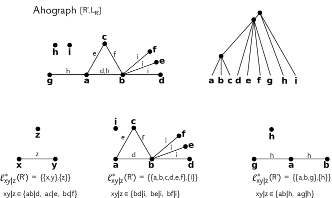
Figure 2: Consider the triple set $R=\{\mathtt{ab|d},\mathtt{ab|h},\mathtt{ac|e},\mathtt{ag|h},\mathtt{bc|f},\mathtt{bc|i},\mathtt{bd|i},\mathtt{be|i},\mathtt{bf|i},\mathtt{bg|h}\}$ and let $R^{\prime}=R\setminus\{\mathtt{bc|i},\mathtt{bg|h}\}$. In this example, $L_{R^{\prime}}=L_{R}$. Clearly, any tree that display $R^{\prime}$ and thus, $\{\mathtt{bc|f},\mathtt{bf|i}\}$, resp., $\{\mathtt{ab|h},\mathtt{ag|h}\}$, must also display $\mathtt{bc|i}$, resp., $\mathtt{bg|h}$ [13]. Thus, $\{\mathtt{bc|i},\mathtt{bg|h}\}\subseteq\operatorname{cl}(R^{\prime})=\operatorname{cl}(R\setminus\{\mathtt{bc|i},\mathtt{bg|h}\})$. Lemma 2.7 implies that $\operatorname{cl}(R^{\prime})=\operatorname{cl}(R)$ and therefore, $R^{\prime}\in\mathfrak{sc}(R)$. The Ahograph $[R^{\prime},L_{R^{\prime}}]$ and a tree $T$ that displays $R^{\prime}$ is shown on the top of this figure. In $[R^{\prime},L_{R^{\prime}}]$ each edge $(x,y)$ is labeled with $z$ that corresponds to the respective triple $\mathtt{xy|z}$ that supports the edge $(x,y)$.
Since $R\subseteq\operatorname{cl}(R)=\operatorname{cl}(R^{\prime})$, the tree $T$ also displays $R$. The respective maximal elements $\ell^{\star}_{\mathtt{xy|z}}(R^{\prime})=\{A,B\}\in\mathfrak{L}^{\star}_{R^{\prime}}(R^{\prime})$ with corresponding Ahographs $[R^{\prime},A\cup B]$ are depicted below. It is easy to verify that each triple $\mathtt{xy|z}\in R^{\prime}$ is a bridge in the respective Ahograph $[R^{\prime},A\cup B]$ and hence, $R^{\prime}$ is minimal (cf. Lemma 4.6). By Theorem 4.8, $R^{\prime}$ has also minimum cardinality. Note, $\operatorname{cl}(R^{\prime})=\operatorname{cl}(R)$ and Theorem 3.9 imply that $\mathfrak{L}^{\star}_{R^{\prime}}(R^{\prime})=\mathfrak{L}^{\star}_{\operatorname{cl}(R)}(\operatorname{cl}(R))=\mathfrak{L}^{\star}_{R}(R)$. In this example, $\mathfrak{L}^{\star}_{R}(R)=\big{\{}\big{\{}\{a,b\},\{d\}\big{\}},\big{\{}\{a,c\},\{e\}\big{\}},\big{\{}\{b,c\},\{f\}\big{\}},\big{\{}\{a,b,c,d,e,f\},\{i\}\big{\}},\big{\{}\{a,b,g\},\{h\}\big{\}}\big{\}}$. In order to determine $\operatorname{cl}(R)$ it suffices to add for each $\{A,B\}\in\mathfrak{L}^{\star}_{R}(R)$ all triples $\mathtt{xy|z}$ with $x,y\in A,z\in B$ or $z\in A,x,y\in B$ to $\operatorname{cl}(R)$ (cf.  Thm.  5.1). Finally, application of Theorem 6.4 shows that $R^{\prime}$ does not identify $T$, since $9=B(T)>|R^{\prime}|=8$ and thus, $\operatorname{cl}(R^{\prime})\neq\mathcal{R}(T)$. Moreover, since $\operatorname{cl}(R)=\operatorname{cl}(R^{\prime})$ neither $R$ identifies $T$.

Theorem 3.9.

For any consistent triple set $R$ it holds that

$$\mathfrak{L}^{\star}_{R}(R)=\mathfrak{L}^{\star}_{\operatorname{cl}(R)}(R)=\mathfrak{L}^{\star}_{\operatorname{cl}(R)}(\operatorname{cl}(R)).\,$$

Proof.

We start with showing $\mathfrak{L}^{\star}_{R}(R)=\mathfrak{L}^{\star}_{\operatorname{cl}(R)}(R)$. Since $R\subseteq\operatorname{cl}(R)$, we also have $\mathfrak{L}^{\star}_{R}(R)\subseteq\mathfrak{L}^{\star}_{\operatorname{cl}(R)}(R)$.

To see that $\mathfrak{L}^{\star}_{\operatorname{cl}(R)}(R)\subseteq\mathfrak{L}^{\star}_{R}(R)$, let $\{A,B\}\in\mathfrak{L}^{\star}_{\operatorname{cl}(R)}(R)$. Hence, there is a triple $\mathtt{ab|c}\in\operatorname{cl}(R)$ with $\ell^{\star}_{\mathtt{ab|c}}(R)=\{A,B\}\in\mathfrak{L}_{\mathtt{ab|c}}(R)$. By definition, $[R,A\cup B]$ has two connected components and at least one contains 2 or more vertices. First, assume for contradiction that there is no triple $\mathtt{a^{\prime}b^{\prime}|c^{\prime}}\in R$ with $\{A,B\}\in\mathfrak{L}_{\mathtt{a^{\prime}b^{\prime}|c^{\prime}}}(R)$. Since $|A|>1$ or $|B|>1$ and $A,B$ are connected components in $[R,A\cup B]$, all edges $(x,y)$ within $\langle A\rangle_{[R,A\cup B]}$ and $\langle B\rangle_{[R,A\cup B]}$ are, therefore, provided by triples $\mathtt{xy|z}\in R$ such that either $x,y,z\in A$ or $x,y,z\in B$. But then $[R,A]$ or $[R,B]$ is connected; contradicting Theorem 2.1. Thus, there must be a triple $\mathtt{a^{\prime}b^{\prime}|c^{\prime}}\in R$ with $\{A,B\}\in\mathfrak{L}_{\mathtt{a^{\prime}b^{\prime}|c^{\prime}}}(R)$. We continue with showing that $\ell^{\star}_{\mathtt{a^{\prime}b^{\prime}|c^{\prime}}}(R)=\{A,B\}$. If this was not the case, then there is an $\ell^{\star}_{\mathtt{a^{\prime}b^{\prime}|c^{\prime}}}(R)=\{A^{\star},B^{\star}\}$ with $|A^{\star}\cup B^{\star}|>|A\cup B|$. Since $\ell^{\star}_{\mathtt{ab|c}}(R)=\{A,B\}\in\mathfrak{L}_{\mathtt{ab|c}}(R)$, one of $A$ and $B$ is containing $a,b$ and the other $c$. Moreover, Lemma 3.5 implies that $A\subseteq A^{\star}$ and $B\subseteq B^{\star}$ or $B\subseteq A^{\star}$ and $A\subseteq B^{\star}$. Taken the latter two arguments together, one of $A^{\star}$ and $B^{\star}$ is containing $a,b$ and the other $c$. Therefore, $\{A^{\star},B^{\star}\}\in\mathfrak{L}_{\mathtt{ab|c}}(R)$. However, since $|A^{\star}\cup B^{\star}|>|A\cup B|$, we have $\ell^{\star}_{\mathtt{ab|c}}(R)\neq\{A,B\}$; a contradiction to the assumption $\ell^{\star}_{\mathtt{ab|c}}(R)=\{A,B\}$. Therefore, $\ell^{\star}_{\mathtt{a^{\prime}b^{\prime}|c^{\prime}}}(R)=\{A,B\}$ and thus, $\{A,B\}\in\mathfrak{L}^{\star}_{R}(R)$. Hence, $\mathfrak{L}^{\star}_{R}(R)=\mathfrak{L}^{\star}_{\operatorname{cl}(R)}(R)$.

Now we show that $\mathfrak{L}^{\star}_{\operatorname{cl}(R)}(R)=\mathfrak{L}^{\star}_{\operatorname{cl}(R)}(\operatorname{cl}(R))$. Let $\{A,B\}=\ell^{\star}_{\mathtt{ab|c}}(R)\in\mathfrak{L}^{\star}_{\operatorname{cl}(R)}(R)$. Since $R\subseteq\operatorname{cl}(R)$ and by Lemma 2.2, $[R,A\cup B]$ is a subgraph of $[\operatorname{cl}(R),A\cup B]$. Since $\{A,B\}=\ell^{\star}_{\mathtt{ab|c}}(R)$, the graph $[R,A\cup B]$ has exactly two connected components $A$ and $B$. Thus, $[\operatorname{cl}(R),A\cup B]$ has at most two connected components. Still, the induced subgraphs $\langle A\rangle$ and $\langle B\rangle$ of $[\operatorname{cl}(R),A\cup B]$ are connected. However, since $\operatorname{cl}(R)$ is consistent we can apply Theorem 2.1 and conclude that $[\operatorname{cl}(R),A\cup B]$ must be disconnected, and thus, has as connected components $A$ and $B$. Therefore, $\{A,B\}\in\mathfrak{L}_{\mathtt{ab|c}}(\operatorname{cl}(R))$. Assume now for contradiction that $\ell^{\star}_{\mathtt{ab|c}}(\operatorname{cl}(R))=\{A^{\star},B^{\star}\}\neq\{A,B\}$. By Lemma 3.5, $|A^{\star}\cup B^{\star}|>|A\cup B|$ and either $A\subseteq A^{\star}$ and $B\subseteq B^{\star}$ or $B\subseteq A^{\star}$ and $A\subseteq B^{\star}$. W.l.o.g. assume that $A\subseteq A^{\star}$ and $B\subseteq B^{\star}$ and $a,b\in A$, $c\in B$. Hence, there is a vertex $d\in(A^{\star}\cup B^{\star})\setminus(A\cup B)$. If $d\in A^{\star}$, then Theorem 2.6 and $a\in A^{\star}$, $c\in B^{\star}$ imply that $\mathtt{ad|c}\in\operatorname{cl}(\operatorname{cl}(R))=\operatorname{cl}(R)$. Again, Theorem 2.6 implies that there is a subset $\mathcal{L}\subseteq L_{R}$ such that $[R,\mathcal{L}]$ has exactly two connected components $A^{\prime}$, $B^{\prime}$ with $a,d\in A^{\prime}$ and $c\in B^{\prime}$. Thus, $\{A^{\prime},B^{\prime}\}\in\mathfrak{L}_{\mathtt{ad|c}}(R)$. Recap that $\{A,B\}\in\mathfrak{L}_{\mathtt{ab|c}}(R)$. Since $A\cap A^{\prime}\neq\emptyset$ and $B\cap B^{\prime}\neq\emptyset$ we can apply Lemma 3.4 and conclude that $\{A\cup A^{\prime},B\cup B^{\prime}\}\in\mathfrak{L}_{\mathtt{ab|c}}(R)$. However, since $d\in A^{\prime}\setminus A$ it holds that $|A\cup A^{\prime}\cup B\cup B^{\prime}|>|A\cup B|$; a contradiction to $\{A,B\}=\ell^{\star}_{\mathtt{ab|c}}(R)$. By similar arguments one derives a contradiction if $d\in B^{\star}$. Thus, $\ell^{\star}_{\mathtt{ab|c}}(\operatorname{cl}(R))=\{A^{\star},B^{\star}\}=\{A,B\}$ and therefore, $\{A,B\}\in\mathfrak{L}^{\star}_{\operatorname{cl}(R)}(\operatorname{cl}(R))$. Hence, $\mathfrak{L}^{\star}_{\operatorname{cl}(R)}(R)\subseteq\mathfrak{L}^{\star}_{\operatorname{cl}(R)}(\operatorname{cl}(R))$.

Finally, let $\{A,B\}=\ell^{\star}_{\mathtt{ab|c}}(\operatorname{cl}(R))\in\mathfrak{L}^{\star}_{\operatorname{cl}(R)}(\operatorname{cl}(R))$. By Lemma 3.3 and since $\mathtt{ab|c}\in\operatorname{cl}(R)$, we have $\mathfrak{L}_{\mathtt{ab|c}}(R)\neq\emptyset$. Thus, there is a maximal element $\ell^{\star}_{\mathtt{ab|c}}(R)=\{A^{\star},B^{\star}\}\in\mathfrak{L}^{\star}_{\operatorname{cl}(R)}(R)\subseteq\mathfrak{L}^{\star}_{\operatorname{cl}(R)}(\operatorname{cl}(R))$. Assume that $\{A,B\}$ and $\{A^{\star},B^{\star}\}$ are distinct. Since both $\{A,B\}$ and $\{A^{\star},B^{\star}\}$ are contained in $\mathfrak{L}^{\star}_{\operatorname{cl}(R)}(\operatorname{cl}(R))$ and $A\cap(A^{\star}\cup B^{\star})\neq\emptyset$, $B\cap(A^{\star}\cup B^{\star})\neq\emptyset$ we can apply Lemma 3.7 and conclude that $A\cup B\subseteq A^{\star}$ or $A\cup B\subseteq B^{\star}$. If $A\cup B\subseteq A^{\star}$, then $a,b,c\in A^{\star}$; a contradiction, since one of $A^{\star}$ and $B^{\star}$ contains $a,b$ and the other $c$. Analogously, $A\cup B\subseteq B^{\star}$ cannot occur. Hence, $\{A,B\}$ and $\{A^{\star},B^{\star}\}$ must be equal and therefore, $\ell^{\star}_{\mathtt{ab|c}}(R)=\ell^{\star}_{\mathtt{ab|c}}(\operatorname{cl}(R))=\{A,B\}\in\mathfrak{L}^{\star}_{\operatorname{cl}(R)}(R)$. Thus, $\mathfrak{L}^{\star}_{\operatorname{cl}(R)}(R)=\mathfrak{L}^{\star}_{\operatorname{cl}(R)}(\operatorname{cl}(R))$. ∎

Theorem 3.10.

Let $R$ be a consistent triple set. If $R^{\prime}\in\mathfrak{sc}(R)$, then $\mathfrak{L}^{\star}_{R}(R)=\mathfrak{L}^{\star}_{R^{\prime}}(R^{\prime})$. In particular, for every $\mathtt{ab|c}\in cl(R)$ and $R^{\prime}\in\mathfrak{sc}(R)$, it holds that $\ell^{\star}_{\mathtt{ab|c}}(R^{\prime})=\ell^{\star}_{\mathtt{ab|c}}(R)$.

Proof.

Let $R^{\prime}\in\mathfrak{sc}(R)$ and thus, $\operatorname{cl}(R^{\prime})=\operatorname{cl}(R)$. Therefore,

$$\mathfrak{L}^{\star}_{R}(R)\stackrel{{\scriptstyle\textrm{Thm.\ \ref{thm:equals}}}}{{=}}\mathfrak{L}^{\star}_{\operatorname{cl}(R)}(\operatorname{cl}(R))=\mathfrak{L}^{\star}_{\operatorname{cl}(R^{\prime})}(\operatorname{cl}(R^{\prime}))\stackrel{{\scriptstyle\textrm{Thm.\ \ref{thm:equals}}}}{{=}}\mathfrak{L}^{\star}_{R^{\prime}}(R^{\prime}).\,$$

Now let $\ell^{\star}_{\mathtt{ab|c}}(R)=\{A^{\star},B^{\star}\}\in\mathfrak{L}^{\star}_{\operatorname{cl}(R)}(R)$. Note, Theorem 3.9 implies that $\mathfrak{L}^{\star}_{\operatorname{cl}(R)}(R)=\mathfrak{L}^{\star}_{R}(R)$ and therefore, $\{A^{\star},B^{\star}\}\in\mathfrak{L}^{\star}_{R}(R)=\mathfrak{L}^{\star}_{R^{\prime}}(R^{\prime})$. Since $\mathtt{ab|c}\in\operatorname{cl}(R)=\operatorname{cl}(R^{\prime})$ we can apply Lemma 3.3 and conclude that $\mathfrak{L}_{\mathtt{ab|c}}(R^{\prime})\neq\emptyset$. Let $\ell^{\star}_{\mathtt{ab|c}}(R^{\prime})=\{A,B\}\in\mathfrak{L}^{\star}_{\operatorname{cl}(R^{\prime})}(R^{\prime})\stackrel{{\scriptstyle\textrm{Thm.\ \ref{thm:equals}}}}{{=}}\mathfrak{L}^{\star}_{R^{\prime}}(R^{\prime})$. Thus, both $\{A^{\star},B^{\star}\}$ and $\{A,B\}$ are contained in $\mathfrak{L}^{\star}_{R^{\prime}}(R^{\prime})$ and $A\cap(A^{\star}\cup B^{\star})\neq\emptyset$, $B\cap(A^{\star}\cup B^{\star})\neq\emptyset$. Now we can argue analogously as in the last part of the proof of Theorem 3.3 to conclude that $\{A,B\}=\{A^{\star},B^{\star}\}$ which implies that $\ell^{\star}_{\mathtt{ab|c}}(R^{\prime})=\ell^{\star}_{\mathtt{ab|c}}(R)$. ∎

4 The Matroid Structure of Minimal and Minimum Representative Triple Sets

By definition, $R^{\prime}\in\operatorname{min}(\mathfrak{sc}(R))$ if and only if there is no subset $R^{\prime\prime}\subsetneq R^{\prime}$ with $\operatorname{cl}(R^{\prime\prime})=\operatorname{cl}(R)$. Furthermore, since any minimum representative triple set is, in particular, minimal, we have $\operatorname{MIN}(\mathfrak{sc}(R))\subseteq\operatorname{min}(\mathfrak{sc}(R))$. The computation of a minimal representative set $R^{\prime}$ of $R$ can be done in combination with the $\mathcal{O}(|R||L_{R}|^{4})$ method to compute the closure [6] in polynomial time as follows: Set $R^{\prime}=R$ and as long as there is a triple $r\in\operatorname{cl}(R^{\prime}\setminus r)$ remove $r$ from $R^{\prime}$. By Lemma 2.7, removal of $r$ from $R^{\prime}$ still preserves $\operatorname{cl}(R)=\operatorname{cl}(R^{\prime})$. However, the computational complexity of finding a minimum representative set $R^{\prime}$ of $R$ is still an open problem. We show that one can determine minimum representative sets in polynomial time. To this end, we give the following

Definition 4.1.

A matroid is an ordered pair $(E,\mathbb{F}_{E})$ consisting of a finite set $E$ and a collection $\mathbb{F}_{E}$ of subsets of $E$ having the following three properties:

• $\emptyset\in\mathbb{F}_{E}$;

• If $I\in\mathbb{F}_{E}$ and $I^{\prime}\subseteq I$, then $I^{\prime}\in\mathbb{F}_{E}$;

• If $I_{1},I_{2}\in\mathbb{F}_{E}$ and $|I_{1}|<|I_{2}|$, then there is an element $x\in I_{2}\setminus I_{1}$ such that $I_{1}\cup\{x\}\in\mathbb{F}_{E}$.

The elements in $\mathbb{F}_{E}$ are called independent in $(E,\mathbb{F}_{E})$. Maximal independent elements of a matroid are called a basis of $(E,\mathbb{F}_{E})$. Every matroid $(E,\mathbb{F}_{E})$ is determined by its collection of its bases. We refer the reader to [50, 40] for more detailed background on matroid theory.

In what follows, we show that $\operatorname{min}(\mathfrak{sc}(R))$ forms the collection of bases of a matroid. In this case, $\operatorname{MIN}(\mathfrak{sc}(R))=\operatorname{min}(\mathfrak{sc}(R))$ since all basis elements of a matroid have the same cardinality [50, 40]. A useful characterization is given by the next result.

Lemma 4.2 ([50, Cor. 1.2.5]).

Let $\mathcal{B}$ be a collection of subsets of $E$. Then $\mathcal{B}$ is the collection of bases of a matroid $(E,\mathbb{F}_{E})$ if and only if it has the following properties:

• $\mathcal{B}\neq\emptyset$;

• If $B_{1},B_{2}\in\mathcal{B}$ and $x\in B_{1}\setminus B_{2}$, then there is an element $y\in B_{2}\setminus B_{1}$ such $(B_{1}\setminus\{x\})\cup\{y\}\in\mathcal{B}$.

Definition 4.3.

In what follows, $(R,\mathbb{F}_{R})$ denotes the ordered pair where

1. $R$ is a consistent triple set and

2. $\mathbb{F}_{R}=\{R^{\prime\prime}\subseteq R^{\prime}\colon R^{\prime}\in\operatorname{min}(\mathfrak{sc}(R))\}$ is the collection of all subsets of the minimal representative sets of $R$.

It is easy to see that $(R,\mathbb{F}_{R})$ is an independent system, that is, it satisfies Conditions (I1) and (I2). Moreover, the collection of bases of $(R,\mathbb{F}_{R})$ is the set $\operatorname{min}(\mathfrak{sc}(R))$. We will utilize Lemma 4.2 to show $\mathcal{B}=\operatorname{min}(\mathfrak{sc}(R))$ satisfies (B1) and (B2). To this end, we give the notion of “bridges” in the Ahograph, that is, triples $\mathtt{ab|c}$ for which the Ahograph $[R\setminus\{\mathtt{ab|c}\},\mathcal{L}]$ has more connected components than $[R,\mathcal{L}]$ . As it turns out, elements $R^{\prime}\in\operatorname{min}(\mathfrak{sc}(R))$ are characterized by the bridge-property of triples $\mathtt{ab|c}\in R^{\prime}$. We first give the following result.

Lemma 4.4.

Let $R$ be a consistent triple set and $R^{\prime}\in\mathfrak{sc}(R)$. Then $R^{\prime}\in\operatorname{min}(\mathfrak{sc}(R))$ if and only if $\operatorname{cl}(R^{\prime})\neq\operatorname{cl}(R^{\prime}\setminus\{r\})$ for all $r\in R^{\prime}$.

Proof.

Let $R$ be a consistent triple set and $R^{\prime}\in\mathfrak{sc}(R)$ and thus, $\operatorname{cl}(R^{\prime})=\operatorname{cl}(R)$. Clearly, if $\operatorname{cl}(R)=cl(R^{\prime})=\operatorname{cl}(R^{\prime}\setminus\{r\})$ for any $r\in R^{\prime}$, then $R^{\prime}\notin\operatorname{min}(\mathfrak{sc}(R))$. Conversely, if $R^{\prime}\notin\operatorname{min}(\mathfrak{sc}(R))$, then there is a subset $R^{\prime\prime}\subsetneq R^{\prime}$ with $\operatorname{cl}(R^{\prime\prime})=\operatorname{cl}(R)$. Since $R^{\prime}\in\mathfrak{sc}(R)$, it also holds that $\operatorname{cl}(R^{\prime})=\operatorname{cl}(R)=\operatorname{cl}(R^{\prime\prime})$. Let $r\in R^{\prime}\setminus R^{\prime\prime}$. Since $R^{\prime\prime}\subseteq R^{\prime}\setminus\{r\}\subsetneq R^{\prime}$, we have $\operatorname{cl}(R^{\prime\prime})\subseteq\operatorname{cl}(R^{\prime}\setminus\{r\})\subseteq\operatorname{cl}(R^{\prime})=\operatorname{cl}(R^{\prime\prime})$ and therefore, $\operatorname{cl}(R^{\prime}\setminus\{r\})=\operatorname{cl}(R^{\prime})$. ∎

Definition 4.5.

Let $R$ be a consistent triple set, $\mathtt{ab|c}\in R$ and $\mathcal{L}\subseteq L_{R}$ such that $a,b,c\in\mathcal{L}$. The triple $\mathtt{ab|c}$ is called bridge in $[R,\mathcal{L}]$ if $a,b$ are in different connected components of $[R\setminus\{\mathtt{ab|c}\},\mathcal{L}]$.

Lemma 4.6.

Let $R$ be a consistent triple set and $R^{\prime}\in\mathfrak{sc}(R)$. Then, $R^{\prime}\in\operatorname{min}(\mathfrak{sc}(R))$ if and only if every $\mathtt{ab|c}\in R^{\prime}$ is a bridge in $[R^{\prime},A\cup B]$ with $\{A,B\}=\ell^{\star}_{\mathtt{ab|c}}(R^{\prime})$. In particular, $[R^{\prime}\setminus\{\mathtt{ab|c}\},A\cup B]$ must have three connected components $\alpha,\beta,\gamma$ with $a\in\alpha$, $b\in\beta$ and $c\in\gamma$, that is, either $A=\alpha\cup\beta$ and $B=\gamma$ or $B=\alpha\cup\beta$ and $A=\gamma$.

Proof.

Let $R^{\prime}\in\operatorname{min}(\mathfrak{sc}(R))$, $\mathtt{ab|c}\in R^{\prime}$ and $\ell^{\star}_{\mathtt{ab|c}}(R^{\prime})=\{A,B\}$. By definition, $[R^{\prime},A\cup B]$ has exactly two connected components, one containing $a,b$ and the other $c$. Assume for contradiction that $\mathtt{ab|c}$ is not a bridge in $[R^{\prime},A\cup B]$. Thus, $a$ and $b$ are still connected by a walk in $[R^{\prime}\setminus\{\mathtt{ab|c}\},A\cup B]$. Note, by Lemma 2.2 the Ahograph $[R^{\prime}\setminus\{\mathtt{ab|c}\},A\cup B]$ is a subgraph of $[R^{\prime},A\cup B]$ that differs from $[R^{\prime},A\cup B]$ only by the edge $(a,b)$. Therefore, $[R^{\prime}\setminus\{\mathtt{ab|c}\},A\cup B]$ still consists of the two connected components $A$ and $B$, one containing $a,b$ and the other $c$. Theorem 2.6 implies that $\{\mathtt{ab|c}\}\in\operatorname{cl}(R^{\prime}\setminus\{\mathtt{ab|c}\})$. Lemma 2.7 implies that $\operatorname{cl}(R^{\prime}\setminus\{\mathtt{ab|c}\})=\operatorname{cl}(R^{\prime})=\operatorname{cl}(R)$; a contradiction to $R^{\prime}\in\operatorname{min}(\mathfrak{sc}(R))$.

Conversely, assume that $R^{\prime}\not\in\operatorname{min}(\mathfrak{sc}(R))$. Thus, there is some triple $\mathtt{ab|c}\in R^{\prime}$ such that $\operatorname{cl}(R^{\prime}\setminus\{\mathtt{ab|c}\})=\operatorname{cl}(R)$. Since $R^{\prime}\in\mathfrak{sc}(R)$, we can apply Theorem 3.10 and conclude that $\ell^{\star}_{\mathtt{ab|c}}(R^{\prime}\setminus\{\mathtt{ab|c}\})=\ell^{\star}_{\mathtt{ab|c}}(R^{\prime})=\{A,B\}$. Thus, $[R^{\prime}\setminus\{\mathtt{ab|c}\},A\cup B]$ has two connected components $A$ and $B$. Therefore, $\mathtt{ab|c}$ is not a bridge in $[R^{\prime},A\cup B]$.

For the last statement, observe that $R^{\prime}\in\operatorname{min}(\mathfrak{sc}(R))$ and $\{A,B\}=\ell^{\star}_{\mathtt{ab|c}}(R^{\prime})$ implies that the graph $[R^{\prime},A\cup B]$ has exactly two connected components, one containing $a,b$ (say $A$) and the other ($B$) contains $c$. Since $\mathtt{ab|c}\in R^{\prime}$ is a bridge in $[R^{\prime},A\cup B]$, $a$ and $b$ are in distinct connected components $\alpha$ and $\beta$ of $[R^{\prime}\setminus\{\mathtt{ab|c}\},A\cup B]$, respectively. However, since only the edge $(a,b)$ has been removed from $[R^{\prime},A\cup B]$ to obtain $[R^{\prime}\setminus\{\mathtt{ab|c}\},A\cup B]$ it is clear that the set $A$ decomposes into these connected components $\alpha,\beta$, i.e., $A=\alpha\cup\beta$. Besides the edge $(a,b)$ no other edge has been removed or added to $[R^{\prime}\setminus\{\mathtt{ab|c}\},A\cup B]$ and thus, $B=\gamma$ is still a connected component in $[R^{\prime}\setminus\{\mathtt{ab|c}\},A\cup B]$ with $c\in\gamma$. ∎

We are now in the position to show that is a matroid.

Theorem 4.7.

If $R$ is a consistent triple set, then $(R,\mathbb{F}_{R})$ is a matroid.

Proof.

In order to show that $(R,\mathbb{F}_{R})$ is a matroid, we show that its collection of bases $\mathcal{B}=\operatorname{min}(\mathfrak{sc}(R))$ satisfies the Conditions (B1) and (B2) of Lemma 4.2. Recall that $(R,\mathbb{F}_{R})$ is an independent system with collection of bases $\mathcal{B}=\operatorname{min}(\mathfrak{sc}(R))$ and $\operatorname{min}(\mathfrak{sc}(R))\neq\emptyset$. Thus, Condition (B1) is trivially satisfied. The proof of Condition (B2) consists of several steps (Claim 1 - 5).

We fix the notion as follows: We assume that $R_{1},R_{2}\in\mathcal{B}$, $\mathtt{ab|c}\in R_{1}\setminus R_{2}$ and $\ell^{\star}_{\mathtt{ab|c}}(R_{1})=\{A,B\}\in\mathfrak{L}^{\star}_{R_{1}}(R_{1})$. Moreover, we will frequently make use of $\mathfrak{L}^{\star}_{R_{1}}(R_{1})=\mathfrak{L}^{\star}_{R}(R)=\mathfrak{L}^{\star}_{R_{2}}(R_{2})$, which is because of $\operatorname{cl}(R_{1})=\operatorname{cl}(R)=\operatorname{cl}(R_{2})$ and Theorem 3.10. Furthermore, Lemma 4.6 implies that $\mathtt{ab|c}$ is a bridge in $[R_{1},A\cup B]$ and that $[R_{1}\setminus\{\mathtt{ab|c}\},A\cup B]$ decomposes into the connected components $\alpha,\beta,\gamma$ with $a\in\alpha$, $b\in\beta$ and $c\in\gamma$. W.l.o.g. we will assume that $a,b\in A,c\in B$ and thus, $A=\alpha\cup\beta$ and $B=\gamma$.

Claim 1:

There exists a triple $\mathtt{a^{\prime}b^{\prime}|c^{\prime}}\in R_{2}$ with $a^{\prime}\in\alpha$, $b^{\prime}\in\beta$ and $c^{\prime}\in\gamma$.

Proof of Claim 1. We begin by showing that there is a triple $\mathtt{a^{\prime}b^{\prime}|c^{\prime}}\in R_{2}$ such that $a^{\prime}\in\alpha$, $b^{\prime}\in\beta$ and $c^{\prime}\in A\cup B$ and then show that $c^{\prime}\in\gamma$.

Assume for contradiction that there is no triple $\mathtt{a^{\prime}b^{\prime}|c^{\prime}}\in R_{2}$ such that $a^{\prime}\in\alpha$, $b^{\prime}\in\beta$ and $c^{\prime}\in A\cup B$. Hence, there is no edge $(x,y)$ in $[R_{2},A\cup B]$ for any $x\in\alpha$ and $y\in\beta$, that is, $\langle A\rangle$ is disconnected in $[R_{2},A\cup B]$. But then $\{A,B\}\notin\mathfrak{L}^{\star}_{R_{2}}(R_{2})$; contradicting $\mathfrak{L}^{\star}_{R_{1}}(R_{1})=\mathfrak{L}^{\star}_{R_{2}}(R_{2})$. Thus there is a triple $\mathtt{a^{\prime}b^{\prime}|c^{\prime}}\in R_{2}$ such that $a^{\prime}\in\alpha$, $b^{\prime}\in\beta$ and $c^{\prime}\in A\cup B$.

We continue to show that $c^{\prime}\in\gamma$. Assume for contradiction that $c^{\prime}\notin\gamma$. Since $\gamma=B$, we have $c^{\prime}\in A$. Let $\ell^{\star}_{\mathtt{a^{\prime}b^{\prime}|c^{\prime}}}(R_{2})=\{A^{\prime},B^{\prime}\}\in\mathfrak{L}^{\star}_{R_{2}}(R_{2})$. Note, since $\mathfrak{L}^{\star}_{R_{1}}(R_{1})=\mathfrak{L}^{\star}_{R_{2}}(R_{2})$ we also have $\{A^{\prime},B^{\prime}\}\in\mathfrak{L}^{\star}_{R_{1}}(R_{1})$ and hence, the graph $[R_{1},A^{\prime}\cup B^{\prime}]$ has the two connected components $A^{\prime}$ and $B^{\prime}$, one containing $a^{\prime},b^{\prime}$ and the other $c^{\prime}$. Furthermore, since $a^{\prime},b^{\prime},c^{\prime}\in A$ we have $A\cap A^{\prime}\neq\emptyset$ and $A\cap B^{\prime}\neq\emptyset$. Hence, $A^{\prime}\cap(A\cup B)\neq\emptyset$ and $B^{\prime}\cap(A\cup B)\neq\emptyset$, and we can apply Lemma 3.7 to conclude that $A^{\prime}\cup B^{\prime}\subseteq A$. Therefore, Lemma 2.2 implies that $[R_{1},A^{\prime}\cup B^{\prime}]\subseteq[R_{1},A\cup B]$. In particular, both $\langle A^{\prime}\rangle\subseteq\langle A\rangle$ and $\langle B^{\prime}\rangle\subseteq\langle A\rangle$ are connected subgraphs in $[R_{1},A\cup B]$. Since $c\notin A$ we have $c\notin A^{\prime}\cup B^{\prime}$ and thus, $[R_{1}\setminus\{\mathtt{ab|c}\},A^{\prime}\cup B^{\prime}\}]=[R_{1},A^{\prime}\cup B^{\prime}]$. Hence, $\langle A^{\prime}\rangle$ and $\langle B^{\prime}\rangle$ remain connected subgraphs in $[R_{1}\setminus\{\mathtt{ab|c}\},A\cup B\}]$. Since $\ell^{\star}_{\mathtt{a^{\prime}b^{\prime}|c^{\prime}}}(R_{2})=\{A^{\prime},B^{\prime}\}$ it holds that either $a^{\prime},b^{\prime}\in A^{\prime}$ and $c^{\prime}\in B^{\prime}$ or $a^{\prime},b^{\prime}\in B^{\prime}$ and $c^{\prime}\in A^{\prime}$. Assume that $a^{\prime},b^{\prime}\in A^{\prime}$. By choice of $\mathtt{a^{\prime}b^{\prime}|c^{\prime}}\in R_{2}$ we have $a^{\prime}\in\alpha$ and $b^{\prime}\in\beta$. Since $A^{\prime},\alpha$ and $\beta$ induce a connected subgraph in $[R_{1}\setminus\{\mathtt{ab|c}\},A\cup B\}]$, respectively, and since $a^{\prime}\in A^{\prime}\cap\alpha$ and $b^{\prime}\in A^{\prime}\cap\beta$, the induced subgraph $\langle A^{\prime}\cup\alpha\cup\beta\rangle$ is connected in $[R_{1}\setminus\{\mathtt{ab|c}\},A\cup B\}]$. However, since $a\in\alpha$ and $b\in\beta$, the triple $\mathtt{ab|c}$ is not a bridge in $[R_{1},A\cup B]$; a contradiction to Lemma 4.6. By analogous arguments one obtains a contradiction if $a^{\prime},b^{\prime}\in B^{\prime}$. Therefore, there is a triple $\mathtt{a^{\prime}b^{\prime}|c^{\prime}}\in R_{2}$ such that $a^{\prime}\in\alpha$, $b^{\prime}\in\beta$ and $c^{\prime}\in\gamma$.

${}_{\textrm{\footnotesize{-- End Proof Claim 1 -- }}}$

In what follows, let $\mathtt{a^{\prime}b^{\prime}|c^{\prime}}\in R_{2}$ be chosen such that $a^{\prime}\in\alpha$, $b^{\prime}\in\beta$ and $c^{\prime}\in\gamma$.

Claim 2:

It holds that $\mathtt{a^{\prime}b^{\prime}|c^{\prime}}\in R_{2}\setminus R_{1}$.

Proof of Claim 2. Recall that $\mathtt{ab|c}\in R_{1}\setminus R_{2}$ and thus, the triples $\mathtt{ab|c}$ and $\mathtt{a^{\prime}b^{\prime}|c^{\prime}}$ must be distinct. Assume for contradiction that $\mathtt{a^{\prime}b^{\prime}|c^{\prime}}\in R_{1}$. In this case, one can easily verify that there are either two edges $(a,b)$ and $(a^{\prime},b^{\prime})$ in $[R_{1},A\cup B]$ connecting $\alpha$ and $\beta$ or, if $(a,b)=(a^{\prime},b^{\prime})$, then the edge $(a,b)$ is supported by two triples. In either case, $\mathtt{ab|c}$ is not a bridge in $[R_{1},A\cup B]$; a contradiction to Lemma 4.6. ${}_{\textrm{\footnotesize{-- End Proof Claim 2 -- }}}$

In what follows, we set $R_{\operatorname{new}}\coloneqq(R_{1}\setminus\{\mathtt{ab|c}\})\cup\{\mathtt{a^{\prime}b^{\prime}|c^{\prime}}\}$.

Claim 3:

It holds that $R_{\operatorname{new}}\in\mathfrak{sc}(R)$.

Proof of Claim 3. Clearly, $R_{\operatorname{new}}\subseteq R$. Hence, in order to show that $R_{\operatorname{new}}\in\mathfrak{sc}(R)$ it remains to show that $\operatorname{cl}(R_{\operatorname{new}})=\operatorname{cl}(R)$. To this end, recap that $[R_{1}\setminus\{\mathtt{ab|c}\},A\cup B]$ has the connected components $\alpha,\beta,\gamma$ with $a,a^{\prime}\in\alpha$, $b,b^{\prime}\in\beta$ and $c,c^{\prime}\in\gamma$. Moreover, Lemma 2.2 implies that $[R_{1}\setminus\{\mathtt{ab|c}\},A\cup B]$ is a subgraph of $[R_{\operatorname{new}},A\cup B]$ and thus, $\langle\alpha\rangle$ and $\langle\beta\rangle$ remain connected subgraphs in $[R_{\operatorname{new}},A\cup B]$. However, since $a^{\prime},b^{\prime},c^{\prime}\in A\cup B$ and $\mathtt{a^{\prime}b^{\prime}|c^{\prime}}\in R_{\operatorname{new}}$ we have an additional edge in $[R_{\operatorname{new}},A\cup B]$ that connects $\langle\alpha\rangle$ and $\langle\beta\rangle$ by the edge $(a^{\prime},b^{\prime})$. Hence, $A=\alpha\cup\beta$ induces a connected subgraph in $[R_{\operatorname{new}},A\cup B]$, while $\langle B\rangle=\langle\gamma\rangle$ remains unchanged and thus still provides a connected component in $[R_{\operatorname{new}},A\cup B]$. In summary, $[R_{\operatorname{new}},A\cup B]$ has two connected components, where $a,b\in A$ and $c\in B$. Theorem 2.6 implies that $\mathtt{ab|c}\in\operatorname{cl}(R_{\operatorname{new}})$. Application of Lemma 2.7 yields $\operatorname{cl}(R_{\operatorname{new}})=\operatorname{cl}(R_{1}\setminus\{\mathtt{ab|c}\})\cup\{\mathtt{a^{\prime}b^{\prime}|c^{\prime}}\})=\operatorname{cl}(R_{1}\cup\{\mathtt{a^{\prime}b^{\prime}|c^{\prime}}\})$. Moreover, it holds that $\operatorname{cl}(R)=\operatorname{cl}(R_{1})\subseteq\operatorname{cl}(R_{1}\cup\{\mathtt{a^{\prime}b^{\prime}|c^{\prime}}\})=\operatorname{cl}(R_{\operatorname{new}})\subseteq\operatorname{cl}(R)$ and therefore, $\operatorname{cl}(R)=\operatorname{cl}(R_{\operatorname{new}})$. Thus, $R_{\operatorname{new}}\in\mathfrak{sc}(R)$. ${}_{\textrm{\footnotesize{-- End Proof Claim 3 -- }}}$

In what follows, we want to show that all triples $\mathtt{xy|z}\in R_{\operatorname{new}}$ are bridges in $[R_{\operatorname{new}},A^{\prime\prime}\cup B^{\prime\prime}]$ where $\ell^{\star}_{\mathtt{xy|z}}(R_{\operatorname{new}})=\{A^{\prime\prime},B^{\prime\prime}\}$ (see Claim 5). In this case, Lemma 4.6 would imply that $R_{\operatorname{new}}\in\operatorname{min}(\mathfrak{sc}(R))$. To this end, however, we first need to prove Claim 4.

Claim 4:

Assume there is a triple $\mathtt{xy|z}\in R_{\operatorname{new}}$ which is not a bridge in $[R_{\operatorname{new}},A^{\prime\prime}\cup B^{\prime\prime}]$ where $\ell^{\star}_{\mathtt{xy|z}}(R_{\operatorname{new}})=\{A^{\prime\prime},B^{\prime\prime}\}$. Then, $\mathtt{xy|z}\neq\mathtt{a^{\prime}b^{\prime}|c^{\prime}}$; $a^{\prime},b^{\prime},c^{\prime}\in A^{\prime\prime}\cup B^{\prime\prime}$; $x$ and $y$ are connected by a path in in $[R_{\operatorname{new}}\setminus\{\mathtt{xy|z}\},A^{\prime\prime}\cup B^{\prime\prime}]$ and every path $P_{xy}$ in $[R_{\operatorname{new}}\setminus\{\mathtt{xy|z}\},A^{\prime\prime}\cup B^{\prime\prime}]$ contains the edge $(a^{\prime},b^{\prime})$; and $\{A^{\prime\prime},B^{\prime\prime}\}\neq\{A,B\}$.

Proof of Claim 4. Assume that $\mathtt{xy|z}\in R_{\operatorname{new}}$ is not a bridge in $[R_{\operatorname{new}},A^{\prime\prime}\cup B^{\prime\prime}]$. First, we show that $\mathtt{xy|z}\neq\mathtt{a^{\prime}b^{\prime}|c^{\prime}}$. Assume for contradiction that $\mathtt{xy|z}=\mathtt{a^{\prime}b^{\prime}|c^{\prime}}$. Now, we show that in this case $\{A^{\prime\prime},B^{\prime\prime}\}=\{A,B\}$. Note, since $\ell^{\star}_{\mathtt{a^{\prime}b^{\prime}|c^{\prime}}}(R_{\operatorname{new}})=\{A^{\prime\prime},B^{\prime\prime}\}$ and $R_{\operatorname{new}}\in\mathfrak{sc}(R)$, we can apply Theorem 3.10 and conclude that $\{A^{\prime\prime},B^{\prime\prime}\}=\ell^{\star}_{\mathtt{a^{\prime}b^{\prime}|c^{\prime}}}(R)$. Since $\ell^{\star}_{\mathtt{ab|c}}(R)=\{A,B\}$, we have $\{A,B\},\{A^{\prime\prime},B^{\prime\prime}\}\in\mathfrak{L}^{\star}_{R}(R)$. Moreover, since by construction $a,b,a^{\prime},b^{\prime}\in A$ and $c^{\prime}\in B$, we have $A\cap(A^{\prime\prime}\cup B^{\prime\prime})\neq\emptyset$ and $B\cap(A^{\prime\prime}\cup B^{\prime\prime})\neq\emptyset$. Hence, we can argue analogously as in the last part of the proof of Theorem 3.3 to conclude that $\{A,B\}=\{A^{\prime\prime},B^{\prime\prime}\}$. Now, since $\mathtt{xy|z}=\mathtt{a^{\prime}b^{\prime}|c^{\prime}}$, the triple $\mathtt{a^{\prime}b^{\prime}|c^{\prime}}$ is not a bridge in $[R_{\operatorname{new}},A^{\prime\prime}\cup B^{\prime\prime}]$. Thus, there is a path $P_{a^{\prime}b^{\prime}}$ in $[R_{\operatorname{new}}\setminus\{\mathtt{a^{\prime}b^{\prime}|c^{\prime}}\},A^{\prime\prime}\cup B^{\prime\prime}]=[R_{\operatorname{new}}\setminus\{\mathtt{a^{\prime}b^{\prime}|c^{\prime}}\},A\cup B]=[R_{1}\setminus\{\mathtt{ab|c}\},A\cup B]$. However, this implies that $P_{a^{\prime}b^{\prime}}$ connects $a^{\prime}\in\alpha$ and $b^{\prime}\in\beta$ in $[R_{1}\setminus\{\mathtt{ab|c}\},A\cup B]$ and therefore, $\mathtt{ab|c}$ is not a bridge in $[R_{1},A\cup B]$; a contradiction to $R_{1}\in\operatorname{min}(\mathfrak{sc}(R))$ and Lemma 4.6. Hence $\mathtt{xy|z}\neq\mathtt{a^{\prime}b^{\prime}|c^{\prime}}$.

We continue to show that every path $P_{xy}$ in $[R_{\operatorname{new}}\setminus\{\mathtt{xy|z}\},A^{\prime\prime}\cup B^{\prime\prime}]$ contains the edge $(a^{\prime},b^{\prime})$. Since $\mathtt{xy|z}\in R_{\operatorname{new}}$ is not a bridge in $[R_{\operatorname{new}},A^{\prime\prime}\cup B^{\prime\prime}]$ there must be a path $P_{xy}$ in $[R_{\operatorname{new}}\setminus\{\mathtt{xy|z}\},A^{\prime\prime}\cup B^{\prime\prime}]$. Assume for contradiction that $P_{xy}$ does not contain the edge $(a^{\prime},b^{\prime})$. Hence, $P_{xy}$ still connects $x$ and $y$ in $[R_{\operatorname{new}}\setminus\{\mathtt{xy|z},\mathtt{a^{\prime}b^{\prime}|c^{\prime}}\},A^{\prime\prime}\cup B^{\prime\prime}]$. Since $R_{\operatorname{new}}\setminus\{\mathtt{xy|z},\mathtt{a^{\prime}b^{\prime}|c^{\prime}}\}\subseteq R_{1}\setminus\{\mathtt{xy|z}\}$ and by Lemma 2.2, the graph $[R_{\operatorname{new}}\setminus\{\mathtt{xy|z},\mathtt{a^{\prime}b^{\prime}|c^{\prime}}\},A^{\prime\prime}\cup B^{\prime\prime}]$ is a subgraph of $[R_{1}\setminus\{\mathtt{xy|z}\},A^{\prime\prime}\cup B^{\prime\prime}]$. Therefore, the path $P_{xy}$ connects $x$ and $y$ in $[R_{1}\setminus\{\mathtt{xy|z}\},A^{\prime\prime}\cup B^{\prime\prime}]$. Note, Theorem 3.10 implies that $\ell^{\star}_{\mathtt{xy|z}}(R_{1})=\{A^{\prime\prime},B^{\prime\prime}\}$. Since $\mathtt{a^{\prime}b^{\prime}|c^{\prime}}\neq\mathtt{xy|z}\in R_{\operatorname{new}}$, we have $\mathtt{xy|z}\in R_{1}$. But then $\mathtt{xy|z}$ is not a bridge in $[R_{1},A^{\prime\prime}\cup B^{\prime\prime}]$; a contradiction to Lemma 4.6.

The latter, in particular, implies that $a^{\prime},b^{\prime}\in A^{\prime\prime}\cup B^{\prime\prime}$. Now, assume for contradiction that $c^{\prime}\notin A^{\prime\prime}\cup B^{\prime\prime}$. Hence, $[R_{\operatorname{new}}\setminus\{\mathtt{xy|z},\mathtt{a^{\prime}b^{\prime}|c^{\prime}}\},A^{\prime\prime}\cup B^{\prime\prime}]=[R_{\operatorname{new}}\setminus\{\mathtt{xy|z}\},A^{\prime\prime}\cup B^{\prime\prime}]$. By the preceding arguments, every path $P_{xy}$ in $[R_{\operatorname{new}}\setminus\{\mathtt{xy|z}\},A^{\prime\prime}\cup B^{\prime\prime}]$ contains the edge $(a^{\prime},b^{\prime})$. Again, since $[R_{\operatorname{new}}\setminus\{\mathtt{xy|z},\mathtt{a^{\prime}b^{\prime}|c^{\prime}}\},A^{\prime\prime}\cup B^{\prime\prime}]$ is a subgraph of $[R_{1}\setminus\{\mathtt{xy|z}\},A^{\prime\prime}\cup B^{\prime\prime}]$ this path is also contained in $[R_{1}\setminus\{\mathtt{xy|z}\},A^{\prime\prime}\cup B^{\prime\prime}]$ and the triple $\mathtt{xy|z}$ is not a bridge in $[R_{1},A^{\prime\prime}\cup B^{\prime\prime}]$; a contradiction to Lemma 4.6 and $\ell^{\star}_{\mathtt{xy|z}}(R_{1})=\{A^{\prime\prime},B^{\prime\prime}\}$. Thus, $c^{\prime}\in A^{\prime\prime}\cup B^{\prime\prime}$

Finally, we show that $\{A^{\prime\prime},B^{\prime\prime}\}\neq\{A,B\}$. Assume for contradiction that $\{A^{\prime\prime},B^{\prime\prime}\}=\{A,B\}$. W.l.o.g. let $A^{\prime\prime}=A=\alpha\cup\beta$ and $B^{\prime\prime}=B=\gamma$. First, we show that neither $x\in\gamma$ nor $y\in\gamma$. Assume w.l.o.g. that $x\in\gamma$. Note the path $P_{xy}$ with edge $(a^{\prime},b^{\prime})$ in $[R_{\operatorname{new}}\setminus\{\mathtt{xy|z}\},A^{\prime\prime}\cup B^{\prime\prime}]$ is also contained $[R_{\operatorname{new}},A^{\prime\prime}\cup B^{\prime\prime}]$. However, since $a^{\prime},b^{\prime}\in A^{\prime\prime}$ and $x\in\gamma=B^{\prime\prime}$ this path $P_{xy}$ connects the two connected components $A^{\prime\prime},B^{\prime\prime}$ in $[R_{\operatorname{new}},A^{\prime\prime}\cup B^{\prime\prime}]$; a contradiction.
We continue to show that neither $x,y\in\alpha$ nor $x,y\in\beta$. Assume for contradiction that $x,y\in\alpha$. Since $[R_{\operatorname{new}}\setminus\{\mathtt{xy|z}\},A^{\prime\prime}\cup B^{\prime\prime}]$ contains a path $P_{xy}$ with edge $(a^{\prime},b^{\prime})$, and $x,y\in\alpha$ there must be a second edge $(a^{\prime\prime},b^{\prime\prime})$ distinct from $(a^{\prime},b^{\prime})$ in $P_{xy}$ where $a^{\prime\prime}\in\alpha,b^{\prime\prime}\in\beta$. Since $R_{\operatorname{new}}\setminus\{\mathtt{xy|z}\}=(R_{1}\setminus\{\mathtt{ab|c},\mathtt{xy|z}\})\cup\{\mathtt{a^{\prime}b^{\prime}|c^{\prime}}\}$, $\{A^{\prime\prime},B^{\prime\prime}\}=\{A,B\}$ and removal of $\{\mathtt{a^{\prime}b^{\prime}|c^{\prime}}\}$ would still preserve the edge $(a^{\prime\prime},b^{\prime\prime})$, this edge $(a^{\prime\prime},b^{\prime\prime})$ must also be contained in $[R_{1}\setminus\{\mathtt{ab|c},\mathtt{xy|z}\},A\cup B]$. Since $[R_{1}\setminus\{\mathtt{ab|c},\mathtt{xy|z}\},A\cup B]$ is a subgraph of $[R_{1}\setminus\{\mathtt{ab|c}\},A\cup B]$, the latter graph contains the edge $(a^{\prime\prime},b^{\prime\prime})$ that connects the components $\alpha$ and $\beta$. But then $\mathtt{ab|c}$ is not a bridge in $[R_{1},A\cup B]$; a contradiction to $R_{1}\in\operatorname{min}(\mathfrak{sc}(R))$ and Lemma 4.6. Hence, $x$ and $y$ cannot be both in $\alpha$, and by similar arguments, not both in $\beta$.
Thus, there are only two cases left: $x\in\alpha$ and $y\in\beta$, or $y\in\alpha$ and $x\in\beta$. Assume w.l.o.g. that $x\in\alpha$ and $y\in\beta$. Since $\mathtt{xy|z}\in R_{1}\setminus\{\mathtt{ab|c}\}$, there must be the edge $(x,y)$ in $[R_{1}\setminus\{\mathtt{ab|c}\},A\cup B]$, in which case $\alpha$ and $\beta$ form a connected component. Again, $\mathtt{ab|c}$ is not a bridge in $[R_{1},A\cup B]$ and we obtain a contradiction to $R_{1}\in\operatorname{min}(\mathfrak{sc}(R))$ and Lemma 4.6.
Therefore, if $\{A^{\prime\prime},B^{\prime\prime}\}=\{A,B\}$, then $x,y\notin\alpha\cup\beta\cup\gamma=A^{\prime\prime}\cup B^{\prime\prime}$; a contradiction since we assumed that $\ell^{\star}_{\mathtt{xy|z}}(R_{\operatorname{new}})=\{A^{\prime\prime},B^{\prime\prime}\}$ and hence, $x,y\in A^{\prime\prime}\cup B^{\prime\prime}$. ${}_{\textrm{\footnotesize{-- End Proof Claim 4 -- }}}$

Claim 5:

$R_{\operatorname{new}}\in\operatorname{min}(\mathfrak{sc}(R))$.

Proof of Claim 5. In order to show that $R_{\operatorname{new}}\in\operatorname{min}(\mathfrak{sc}(R))$ we use Lemma 4.6 and show that each triple $\mathtt{xy|z}\in R_{\operatorname{new}}$ must be a bridge in $[R_{\operatorname{new}},A^{\prime\prime}\cup B^{\prime\prime}]$ where $\ell^{\star}_{\mathtt{xy|z}}(R_{\operatorname{new}})=\{A^{\prime\prime},B^{\prime\prime}\}$.

Assume for contradiction, that there is a triple $\mathtt{xy|z}\in R_{\operatorname{new}}$ that is not a bridge in $[R_{\operatorname{new}},A^{\prime\prime}\cup B^{\prime\prime}]$. Claim 4. implies that $\mathtt{xy|z}\neq\mathtt{a^{\prime}b^{\prime}|c^{\prime}}$ and thus, in particular, $\mathtt{xy|z}\in R_{1}\setminus\{\mathtt{ab|c}\}$. Moreover, $a^{\prime},b^{\prime},c^{\prime}\in A^{\prime\prime}\cup B^{\prime\prime}$, $\{A^{\prime\prime},B^{\prime\prime}\}\neq\{A,B\}$ and every path $P_{xy}$ in $[R_{\operatorname{new}}\setminus\{\mathtt{xy|z}\},A^{\prime\prime}\cup B^{\prime\prime}]$ contains the edge $(a^{\prime},b^{\prime})$. Recap that $a,a^{\prime}\in\alpha$, $b,b^{\prime}\in\beta$, $c,c^{\prime}\in\gamma$, $A=\alpha\cup\beta$ and $B=\gamma$.

Recap that $\ell^{\star}_{\mathtt{ab|c}}(R_{1})=\{A,B\}\in\mathfrak{L}^{\star}_{R_{1}}(R_{1})$. Claim 3 implies that $R_{\operatorname{new}}\in\mathfrak{sc}(R)$. Thus, we can apply Theorem 3.10 and conclude that $\{A^{\prime\prime},B^{\prime\prime}\}=\ell^{\star}_{\mathtt{xy|z}}(R_{\operatorname{new}})=\ell^{\star}_{\mathtt{xy|z}}(R)=\ell^{\star}_{\mathtt{xy|z}}(R_{1})$. Hence, $\{A^{\prime\prime},B^{\prime\prime}\}\in\mathfrak{L}^{\star}_{R_{1}}(R_{1})$. Moreover, since $a^{\prime},b^{\prime},c^{\prime}\in A^{\prime\prime}\cup B^{\prime\prime}$ as well as $a^{\prime},b^{\prime}\in A$ and $c^{\prime}\in B$ it holds that $A\cap(A^{\prime\prime}\cup B^{\prime\prime})\neq\emptyset$ and $B\cap(A^{\prime\prime}\cup B^{\prime\prime})\neq\emptyset$. Thus, we can apply Lemma 3.7 and conclude that $A\cup B\subseteq A^{\prime\prime}$ or $A\cup B\subseteq B^{\prime\prime}$. W.l.o.g. assume $A\cup B\subseteq A^{\prime\prime}$.

Denote one of the paths in $[R_{\operatorname{new}}\setminus\{\mathtt{xy|z}\},A^{\prime\prime}\cup B^{\prime\prime}]$ that connect $x$ and $y$ by $P_{xy}$. Claim 4 implies that $P_{xy}$ contains the edge $(a^{\prime},b^{\prime})$. Since $a^{\prime},b^{\prime}\in A^{\prime\prime}$ it must hold that $x,y\in A^{\prime\prime}$ as otherwise $P_{xy}$ would connect $A^{\prime\prime}$ and $B^{\prime\prime}$ in $[R_{\operatorname{new}},A^{\prime\prime}\cup B^{\prime\prime}]$. Therefore, $z\in B^{\prime\prime}$ and hence $z\notin A\cup B$. Since $P_{xy}$ contains the edge $(a^{\prime},b^{\prime})$, it can be decomposed into the paths $P_{xa^{\prime}}$ and $P_{b^{\prime}y}$ (resp. $P_{xb^{\prime}}$ and $P_{ya^{\prime}}$) and the edge $(a^{\prime},b^{\prime})$. W.l.o.g. assume that $P_{xy}$ is composed of $P_{xa^{\prime}}$, $(a^{\prime},b^{\prime})$ and $P_{b^{\prime}y}$. Note, since neither $P_{xa^{\prime}}$ nor $P_{b^{\prime}y}$ contains the edge $(a^{\prime},b^{\prime})$, we can conclude that both paths are contained in $[R_{\operatorname{new}}\setminus\{\mathtt{xy|z},\mathtt{a^{\prime}b^{\prime}|c^{\prime}}\},A^{\prime\prime}\cup B^{\prime\prime}]=[R_{1}\setminus\{\mathtt{xy|z},\mathtt{ab|c}\},A^{\prime\prime}\cup B^{\prime\prime}]\subseteq[R_{1}\setminus\{\mathtt{xy|z}\},A^{\prime\prime}\cup B^{\prime\prime}]$. Furthermore, since $\alpha$ and $\beta$ induce connected subgraphs in $[R_{1}\setminus\mathtt{ab|c},A\cup B]$ and $a,a^{\prime}\in\alpha$, $b,b^{\prime}\in\beta$, there are paths $P_{aa^{\prime}}$ and $P_{bb^{\prime}}$ in $[R_{1}\setminus\{\mathtt{ab|c}\},A\cup B]$. Since $z\notin A\cup B$ and $A\cup B\subseteq A^{\prime\prime}$, we have $[R_{1}\setminus\{\mathtt{ab|c}\},A\cup B]=[R_{1}\setminus\{\mathtt{ab|c},\mathtt{xy|z}\},A\cup B]\subseteq[R_{1}\setminus\{\mathtt{xy|z}\},A^{\prime\prime}\cup B^{\prime\prime}]$. Hence, the paths $P_{aa^{\prime}}$ and $P_{bb^{\prime}}$ are also contained in $[R_{1}\setminus\{\mathtt{xy|z}\},A^{\prime\prime}\cup B^{\prime\prime}]$. In summary, $[R_{1}\setminus\{\mathtt{xy|z}\},A^{\prime\prime}\cup B^{\prime\prime}]$ contains the paths $P_{aa^{\prime}}$, $P_{bb^{\prime}}$, $P_{xa^{\prime}}$ and $P_{b^{\prime}y}$ but also the edge $(a,b)$, since $\mathtt{ab|c}\in R_{1}\setminus\{\mathtt{xy|z}\}$ and $a,b,c\in A\cup B\subseteq A^{\prime\prime}$. Hence, we can combine the four paths and the edge $(a,b)$ to a walk in $[R_{1}\setminus\{\mathtt{xy|z}\},A^{\prime\prime}\cup B^{\prime\prime}]$ that connects $x$ and $y$. However, this implies that $\mathtt{xy|z}$ is not a bridge in $[R_{1},A^{\prime\prime}\cup B^{\prime\prime}]$; a contradiction to $\ell^{\star}_{\mathtt{xy|z}}(R_{1})=\{A^{\prime\prime},B^{\prime\prime}\}$ and Lemma 4.6.

In summary, for all cases for which there is a triple $\mathtt{xy|z}\in R_{\operatorname{new}}$ that is not a bridge in $[R_{\operatorname{new}},A^{\prime\prime}\cup B^{\prime\prime}]$ we obtain a contradiction. Hence, each triple $\mathtt{xy|z}\in R_{\operatorname{new}}$ must be a bridge in $[R_{\operatorname{new}},A^{\prime\prime}\cup B^{\prime\prime}]$ and we can apply Lemma 4.6 to conclude that $R_{\operatorname{new}}\in\operatorname{min}(\mathfrak{sc}(R))$. ${}_{\textrm{\footnotesize{-- End Proof Claim 5 -- }}}$

We have shown that for any $R_{1},R_{2}\in\mathcal{B}=\operatorname{min}(\mathfrak{sc}(R))$ and $\mathtt{ab|c}\in R_{1}\setminus R_{2}$ there is a triple $\mathtt{a^{\prime}b^{\prime}|c^{\prime}}\in R_{2}\setminus R_{1}$ such that $R_{\operatorname{new}}=(R_{1}\setminus\{\mathtt{ab|c}\})\cup\{\mathtt{a^{\prime}b^{\prime}|c^{\prime}}\}\in\mathcal{B}$. Hence, we can apply Lemma 4.2 to conclude that $(R,\mathbb{F}_{R})$ is a matroid. ∎

In order to avoid confusion, we emphasize that the closure operator $\operatorname{cl}(R)$ for rooted triple sets $R$ defined here is not a matroid closure operator $\operatorname{cl}_{M}$ [50, 40]. Note, since $M=(R,\mathbb{F}_{R})$ is a matroid, the following property must be satisfied for $\operatorname{cl}_{M}$, cf. [50, Lemma 1.4.3]:

$$X\subseteq R,r\in R\text{ and }r^{\prime}\in\operatorname{cl}_{M}(X\cup\{r\})\setminus\operatorname{cl}_{M}(X)\implies r\in\operatorname{cl}_{M}(X\cup\{r^{\prime}\}).\,$$

To see that $\operatorname{cl}(R)$ does not fulfill this property in general, consider the example in Figure 1. To recap, $R_{1}=\{\mathtt{ab|c},\mathtt{ac|d}\}$, $R_{3}=\{\mathtt{ac|d},\mathtt{bc|d}\}$ and $\operatorname{cl}(R_{1})=\operatorname{cl}(R)=\{\mathtt{ab|c},\mathtt{ac|d},\mathtt{bc|d},\mathtt{ab|d}\}$, but $\operatorname{cl}(R_{3})=\operatorname{cl}(R)\setminus\mathtt{ab|c}$. Now, put $X=\{\mathtt{ac|d}\}$ and $r=\mathtt{ab|c}$. Thus, $r^{\prime}=\mathtt{bc|d}\in\operatorname{cl}(X\cup\{r\})\setminus\operatorname{cl}(X)=\operatorname{cl}(R_{1})\setminus\{\mathtt{ab|c}\}$. However, $r=\mathtt{ab|c}\notin\operatorname{cl}(X\cup\{r^{\prime}\})=\operatorname{cl}(R_{3})$. The latter result has already been observed by David Bryant [5], however, the matroid structure of $(R,\mathbb{F}_{R})$ was not discovered.

Note, each minimum representative set $R^{\prime}\in\operatorname{MIN}(\mathfrak{sc}(R))$ is also minimal. Thus, $\operatorname{MIN}(\mathfrak{sc}(R))\subseteq\operatorname{min}(\mathfrak{sc}(R))$. However, since $(R,\mathbb{F}_{R})$ is a matroid with collection of bases $\operatorname{min}(\mathfrak{sc}(R))$, all elements in $\operatorname{min}(\mathfrak{sc}(R))$ have the same cardinality [50]. Therefore, all basis elements of the matroid $(R,\mathbb{F}_{R})$ are of minimum size. We summarize this observation in the following

Theorem 4.8.

If $R$ is a consistent triple set, then $\operatorname{min}(\mathfrak{sc}(R))=\operatorname{MIN}(\mathfrak{sc}(R))$.

In order to find a minimum representative set $R^{\prime}$ of $R$ one can apply a simple greedy algorithm. Algorithm 1 computes a basis element of the matroid $(R,\mathbb{F}_{R})$ and can easily be adapted to find maximum weighted bases, an issue that might be important for applications in phylogenetics, where the weight of a rooted triple corresponds to a statistical confidence value or any other measure associated with the underlying triples.

Lemma 4.9.

Algorithm 1 computes a subset $R^{\prime}\subseteq R$ with $\operatorname{cl}(R^{\prime})=\operatorname{cl}(R)$ of minimum size in $\mathcal{O}(|R|^{2}|L_{R}|)$.

Proof.

By Lemma 2.5, it suffices to decide whether a triple $\mathtt{ab|c}$ is contained in $\operatorname{cl}(R\setminus(R_{\operatorname{tmp}}\cup\{\mathtt{ab|c}\}))$ by the two consistency checks in the IF-condition.

Let $R_{\operatorname{tmp}}=\{r_{1},\dots,r_{k}\}$ where the indices of the triples are chosen w.r.t. the order in which they are added to $R_{\operatorname{tmp}}$. By construction, $r_{i}\in R_{\operatorname{tmp}}$ if $r_{i}\in\operatorname{cl}(R\setminus\{r_{1},\dots,r_{i}\})$. Lemma 2.7 implies that for the first triple $r_{1}\in\operatorname{cl}(R\setminus\{r_{1}\})$ it holds that $\operatorname{cl}(R\setminus\{r_{1}\})=\operatorname{cl}(R)$. Next, $r_{2}$ is added to $R_{\operatorname{tmp}}$ that is, $r_{2}\in\operatorname{cl}(R\setminus\{r_{1},r_{2}\})$ and again by Lemma 2.7, $\operatorname{cl}(R\setminus\{r_{1},r_{2}\})=\operatorname{cl}(R\setminus\{r_{1}\})=\operatorname{cl}(R)$. Inductively, when $r_{k}$ is chosen we have $r_{k}\in\operatorname{cl}(R\setminus R_{\operatorname{tmp}}\})=\operatorname{cl}(R\setminus\{r_{1},\dots,r_{k-1}\})=\cdots=\operatorname{cl}(R\setminus\{r_{1}\})=\operatorname{cl}(R)$. Since by construction, $R_{\min}=R\setminus R_{\operatorname{tmp}}$, it holds that $\operatorname{cl}(R_{\min})=\operatorname{cl}(R\setminus R_{\operatorname{tmp}})=\operatorname{cl}(R)$.

We continue to show that $R_{\min}\in\operatorname{min}(\mathfrak{sc}(R))$. Assume for contradiction that there is a subset $R^{\prime\prime}\subsetneq R_{\min}$ with $\operatorname{cl}(R^{\prime\prime})=\operatorname{cl}(R)$. Note, $R^{\prime\prime}=R_{\min}\setminus R^{\prime}$ for some non-empty subset $R^{\prime}\subseteq R_{\min}$. Thus, $\operatorname{cl}(R_{\min}\setminus R^{\prime})=\operatorname{cl}(R)=\operatorname{cl}(R_{\min})$. Lemma 2.7 implies that there is a triple $r\in R^{\prime}$ such that $\operatorname{cl}(R_{\min}\setminus\{r\})=\operatorname{cl}(R_{\min})$. Note, since $r\in R^{\prime}\subseteq R_{\min}=R\setminus R_{\operatorname{tmp}}$ it holds that $r\notin R_{\operatorname{tmp}}$.

Consider the step when $r$ is chosen in Alg. 1. If $R_{\operatorname{tmp}}=\emptyset$ before this step, we would have $r\notin\operatorname{cl}(R\setminus\{r\})$, since $r$ is not added to $R_{\operatorname{tmp}}$. However, since $r\in R_{\min}$ and $R_{\min}\setminus\{r\}\subseteq R\setminus\{r\}$ and it must hold that $r\in\operatorname{cl}(R_{\min})=\operatorname{cl}(R_{\min}\setminus\{r\})\subseteq\operatorname{cl}(R\setminus\{r\})$; a contradiction. If $R_{\operatorname{tmp}}$ is not empty and thus, $R_{\operatorname{tmp}}=\{r_{1},\dots,r_{i}\}$ before the step when $r$ is chosen in Alg. 1, we would have $r\notin\operatorname{cl}(R\setminus\{r_{1},\dots,r_{i},r\})$, since $r$ is not added to $R_{\operatorname{tmp}}$. However, since $r\in R_{\min}$ and $R_{\min}\setminus\{r\}=R\setminus\{r_{1},\dots,r_{k},r\}\subseteq R\setminus\{r_{1},\dots,r_{i},r\}$ it must hold that $r\in\operatorname{cl}(R_{\min})=\operatorname{cl}(R_{\min}\setminus\{r\})\subseteq\operatorname{cl}(R\setminus\{r_{1},\dots,r_{i},r\})$; a contradiction. Therefore, $R_{\min}$ is minimal and we can apply Theorem 4.8 to conclude that $R_{\min}$ is of minimum size.

Concerning the time complexity, observe that the for-loop runs $|R|$ times. In each step of the for-loop, we have to check for consistency which can be done with BUILD in $\mathcal{O}(|R||L_{R}|)$ time. Thus, we end in an overall time complexity $\mathcal{O}(|R|^{2}|L_{R}|)$. ∎

Algorithm 1 GREEDY for Minimal/Minimum Representative Triple Sets

1:Consistent triple set $R$;

2:Minimal Representative Triple set $R_{\min}$;

3:$R_{\operatorname{tmp}}\leftarrow\emptyset$;

4:for all $\mathtt{ab|c}\in R$ do

5:    $R^{\prime}\leftarrow R\setminus R_{\operatorname{tmp}}$;

6:    if $R^{\prime}\setminus\{\mathtt{ab|c}\}\cup\{\mathtt{bc|a}\}$ and $R^{\prime}\setminus\{\mathtt{ab|c}\}\cup\{\mathtt{ac|b}\}$ are not consistent then $\triangleright$ Thus, $\mathtt{ab|c}\in\operatorname{cl}(R\setminus(R_{\operatorname{tmp}}\cup\{\mathtt{ab|c}\}))$

7:        $R_{\operatorname{tmp}}\leftarrow R_{\operatorname{tmp}}\cup\{\mathtt{ab|c}\}$;     

8:return $R_{\min}\leftarrow R\setminus R_{\operatorname{tmp}}$;

As a consequence, we obtain the following result:

Theorem 4.10.

Let $R_{1},R_{2}$ be consistent triple sets such that $\operatorname{cl}(R_{1})=\operatorname{cl}(R_{2})$. For each $R^{\prime}_{1}\in\operatorname{min}(\mathfrak{sc}(R_{1}))$ and $R^{\prime}_{2}\in\operatorname{min}(\mathfrak{sc}(R_{2}))$ it holds that $|R^{\prime}_{1}|=|R^{\prime}_{2}|$.

Proof.

Let $R_{1}$ and $R_{2}$ be consistent triple sets such that $\operatorname{cl}(R_{1})=\operatorname{cl}(R_{2})$. Set $R=\operatorname{cl}(R_{1})$ and apply the greedy method with input $R$. Since $\operatorname{cl}(R_{1})=\operatorname{cl}(R)$ and since the choice of the triples assigned to $R_{\operatorname{tmp}}$ is arbitrary as long as $\operatorname{cl}(R\setminus R_{\operatorname{tmp}})=\operatorname{cl}(R)$, it is possible to obtain greedily a set $R_{\operatorname{tmp}}$ for which $R^{\prime}=R_{1}=R\setminus R_{\operatorname{tmp}}\subseteq R$ (in Step 5 of Alg. 1). Now Alg. 1 continues with $R_{1}$ in order to find a subset $R^{\prime}\subseteq R_{1}$ such that $R^{\prime}\in\operatorname{min}(\mathfrak{sc}(R))=\operatorname{min}(\mathfrak{sc}(\operatorname{cl}(R_{1})))$. Note, $R^{\prime}\in\operatorname{min}(\mathfrak{sc}(R_{1}))$ as otherwise there would be a subset $R^{\prime\prime}\subsetneq R^{\prime}\subseteq R_{1}\subseteq\operatorname{cl}(R_{1})$ such that $\operatorname{cl}(R^{\prime\prime})=\operatorname{cl}(R_{1})$; a contradiction to $R^{\prime}\in\operatorname{min}(\mathfrak{sc}(\operatorname{cl}(R_{1})))$ and the correctness of Alg. 1. Hence, for any $R^{\prime}_{1}\in\operatorname{min}(\mathfrak{sc}(\operatorname{cl}(R_{1})))$ with $R^{\prime}_{1}\subseteq R_{1}$ we also have $R^{\prime}_{1}\in\operatorname{min}(\mathfrak{sc}(R_{1}))$. The same applies to $R_{2}$, that is, $R^{\prime}_{2}\in\operatorname{min}(\mathfrak{sc}(R_{2}))$ for any $R^{\prime}_{2}\in\operatorname{min}(\mathfrak{sc}(\operatorname{cl}(R_{2})))$ with $R^{\prime}_{2}\subseteq R_{2}$. Since $\operatorname{cl}(R_{1})=\operatorname{cl}(R_{2})$, it holds that $\operatorname{min}(\mathfrak{sc}(\operatorname{cl}(R_{1})))=\operatorname{min}(\mathfrak{sc}(\operatorname{cl}(R_{2})))$. The latter together with Theorem 4.8 implies that $|R^{\prime}_{1}|=|R^{\prime}_{2}|$. ∎

5 Computing the Closure

The currently fastest algorithm to determine the closure has a time complexity of $\mathcal{O}(|R||L_{R}|^{4})$ and was proposed by Bryant and Steel [6]. In this section, we provide a novel and efficient algorithm to compute the closure. This method is based on the techniques we used to prove the matroid structure. In particular, the proposed algorithm will rely on computing the set $\mathfrak{L}^{\star}_{R}(R)$ and usage of the following theorem.

Theorem 5.1.

Let $R$ be a consistent triple set and define $\mathcal{R}_{A,B}=\{\mathtt{ab|c}\colon a,b\in A,c\in B\text{ or }a,b\in B,c\in A\}$ for any $A,B\subseteq L_{R}$. Then,

$$\operatorname{cl}(R)=\bigcup_{\{A,B\}\in\mathfrak{L}^{\star}_{R}(R)}\mathcal{R}_{A,B}.\,$$

Moreover, for any distinct $\{A,B\},\{A^{\prime},B^{\prime}\}\in\mathfrak{L}^{\star}_{R}(R)$ it holds that $\mathcal{R}_{A,B}\cap\mathcal{R}_{A^{\prime},B^{\prime}}=\emptyset$. In particular,

$$\sum_{\{A,B\}\in\mathfrak{L}^{\star}_{R}(R)}|R_{A,B}|\leq|L_{R}|^{3}.\,$$

Proof.

Theorem 2.6 immediately implies that $\bigcup_{\{A,B\}\in\mathfrak{L}^{\star}_{R}(R)}\mathcal{R}_{A,B}\subseteq\operatorname{cl}(R)$. Thus, it remains to show that $\operatorname{cl}(R)\subseteq\bigcup_{\{A,B\}\in\mathfrak{L}^{\star}_{R}(R)}\mathcal{R}_{A,B}$. Let $\mathtt{ab|c}\in\operatorname{cl}(R)$. Lemma 3.3 implies that $\mathfrak{L}_{\mathtt{ab|c}}(R)\neq\emptyset$. Thus, there is also a maximal element $\ell^{\star}_{\mathtt{ab|c}}(R)=\{A,B\}\in\mathfrak{L}^{\star}_{\operatorname{cl}(R)}(R)$. Theorem 3.9 implies that $\mathfrak{L}^{\star}_{\operatorname{cl}(R)}(R)=\mathfrak{L}^{\star}_{R}(R)$ and hence, it particularly holds that $\{A,B\}\in\mathfrak{L}^{\star}_{R}(R)$ for which $\mathtt{ab|c}\in\mathcal{R}_{A,B}$. Therefore, $\mathtt{ab|c}\in\bigcup_{\{A,B\}\in\mathfrak{L}^{\star}_{R}(R)}\mathcal{R}_{A,B}$ and thus, $\operatorname{cl}(R)=\bigcup_{\{A,B\}\in\mathfrak{L}^{\star}_{R}(R)}\mathcal{R}_{A,B}$.

We continue by showing that for any distinct $\{A,B\},\{A^{\prime},B^{\prime}\}\in\mathfrak{L}^{\star}_{R}(R)$ we have $\mathcal{R}_{A,B}\cap\mathcal{R}_{A^{\prime},B^{\prime}}=\emptyset$. Assume for contradiction that $\mathtt{ab|c}\in\mathcal{R}_{A,B}\cap\mathcal{R}_{A^{\prime},B^{\prime}}$ for some distinct $\{A,B\},\{A^{\prime},B^{\prime}\}\in\mathfrak{L}^{\star}_{R}(R)$. Thus, $A\cap(A^{\prime}\cup B^{\prime})\neq\emptyset$ and $B\cap(A^{\prime}\cup B^{\prime})\neq\emptyset$, as well as $A^{\prime}\cap(A\cup B)\neq\emptyset$ and $B^{\prime}\cap(A\cup B)\neq\emptyset$. Lemma 3.7 implies that either $A\cup B\subseteq A^{\prime}$ or $A\cup B\subseteq B^{\prime}$ and either $A^{\prime}\cup B^{\prime}\subseteq A$ or $A^{\prime}\cup B^{\prime}\subseteq B$. W.l.o.g. assume that $A^{\prime}\cup B^{\prime}\subseteq A$ and therefore, $A^{\prime},B^{\prime}\subseteq A$. If $A\cup B\subseteq A^{\prime}$ (resp. $A\cup B\subseteq B^{\prime}$), then $B^{\prime}\subseteq A^{\prime}$ (resp. $A^{\prime}\subseteq B^{\prime}$); a contradiction to the disjointedness of $A^{\prime},B^{\prime}$. Hence, $\mathcal{R}_{A,B}\cap\mathcal{R}_{A^{\prime},B^{\prime}}=\emptyset$.

Finally, since $\mathcal{R}_{A,B}\cap\mathcal{R}_{A^{\prime},B^{\prime}}=\emptyset$ are disjoint for distinct $\{A,B\},\{A^{\prime},B^{\prime}\}\in\mathfrak{L}^{\star}_{R}(R)$, the closure $\operatorname{cl}(R)$ is the disjoint union $\uplus_{\{A,B\}\in\mathfrak{L}^{\star}_{R}(R)}\mathcal{R}_{A,B}$ and therefore, $|\operatorname{cl}(R)|=\sum_{\{A,B\}\in\mathfrak{L}^{\star}_{R}(R)}|R_{A,B}|$. Since $\operatorname{cl}(R)$ can have at most $|L_{R}|^{3}$ triples, that is, one triple for each of three-element subsets of $L_{R}$, the assertion follows. ∎

Lemma 5.2.

Let $R$ be a consistent triple set and $\mathtt{ab|c}\in R$. Moreover, assume that there is a subset $\mathcal{L}\subseteq L_{R}$ with $a,b,c\in\mathcal{L}$ such that $a,b$ are contained together in some connected component $\mathcal{C}_{a,b}$ of $[R,\mathcal{L}]$. Let $\mathcal{C}_{c}$ denote the connected component in $[R,\mathcal{L}]$ that contains $c$. Note, we don’t claim that $\mathcal{C}_{a,b}\neq\mathcal{C}_{c}$.

Then, $\mathcal{L}^{\prime}\subseteq\mathcal{C}_{a,b}\cup\mathcal{C}_{c}$ for all $\mathcal{L}^{\prime}\subseteq\mathcal{L}$ for which $[R,\mathcal{L}^{\prime}]$ has exactly two connected components, one containing $a,b$ and the other $c$.

Proof.

Assume for contradiction that there is a subset $\mathcal{L}^{\prime}=A\cup B\subseteq\mathcal{L}$ such that $[R,\mathcal{L}^{\prime}]$ has exactly two connected components $A$ and $B$ with $a,b\in A$ and $c\in B$, but $\mathcal{L}^{\prime}\not\subseteq\mathcal{C}_{a,b}\cup\mathcal{C}_{c}$. Thus, there is a vertex $d\in\mathcal{L}^{\prime}\setminus(\mathcal{C}_{a,b}\cup\mathcal{C}_{c})$. Therefore, $d$ is either contained in $A$ or in $B$, that is, there is either a path $P_{da}$ or $P_{dc}$ in $[R,\mathcal{L}^{\prime}]$. Since $[R,\mathcal{L}^{\prime}]$ is a subgraph of $[R,\mathcal{L}]$ these paths are also contained in $[R,\mathcal{L}]$. But then, $d\in\mathcal{C}_{a,b}$ or $d\in\mathcal{C}_{c}$; a contradiction. ∎

Algorithm 2 Compute $\mathfrak{L}^{\star}_{R}(R)$

1:A consistent triple set $R$;

2:$\mathfrak{L}^{\star}_{R}(R)$;

3:$\mathfrak{L}^{\star}_{R}(R)\leftarrow\emptyset$;

4:for all $\mathtt{ab|c}\in R$ do

5:    $\mathcal{C}\leftarrow L_{R}$;

6:    while $[R,\mathcal{C}]$ does not have exactly two connected components $A,B$, one containing $a,b$ and the other $c$ do

7:        $\mathcal{C}_{a,b}\leftarrow$ connected component in $[R,\mathcal{C}]$ that contains $a,b$;

8:        $\mathcal{C}_{c}\leftarrow$ connected component in $[R,\mathcal{C}]$ that contains $c$;

9:        $\mathcal{C}\leftarrow\mathcal{C}_{a,b}\cup\mathcal{C}_{c}$;     

10:    $\mathfrak{L}^{\star}_{R}(R)\leftarrow\mathfrak{L}^{\star}_{R}(R)\cup\{A,B\}$;

11:return $\mathfrak{L}^{\star}_{R}(R)\leftarrow\mathfrak{L}^{\star}_{R}(R)$;

Algorithm 3 Compute Closure $\operatorname{cl}(R)$

1:A consistent triple set $R$;

2:$\operatorname{cl}(R)$;

3:Compute $\mathfrak{L}^{\star}_{R}(R)$ with Algorithm 2;

4:$\operatorname{cl}(R)\leftarrow\emptyset$;

5:for all $\{A,B\}\in\mathfrak{L}^{\star}_{R}(R)$ do

6:    Compute $\mathcal{R}_{A,B}$ (cf.  Theorem 5.1);

7:    $\operatorname{cl}(R)\leftarrow\operatorname{cl}(R)\cup\mathcal{R}_{A,B}$;

8:return $\operatorname{cl}(R)$;

The latter lemma immediately offers a way to compute $\mathfrak{L}^{\star}_{R}(R)$ that is summarized in Algorithm 2. For each triple $\mathtt{ab|c}\in R$ start with $[R,L_{R}]$. If $[R,L_{R}]$ has already two connected components $A$ and $B$, one containing $a,b$ and the other $c$, then $L_{R}=A\cup B$ clearly maximizes $|A\cup B|$. Thus, $\{A,B\}=\ell^{\star}_{\mathtt{ab|c}}(R)\in\mathfrak{L}^{\star}_{R}(R)$. If $[R,L_{R}]$ does not have these two connected components $A$ and $B$, it is, however, still disconnected (cf.  Theorem 2.1). Hence, $[R,L_{R}]$ has two or more connected components. Nevertheless, $a,b$ must be in one connected component $\mathcal{C}_{a,b}$ due to the edge $(a,b)$ implied by $\mathtt{ab|c}\in R$. Moreover, there is a connected component $\mathcal{C}_{c}$ that contains $c$. Note, $\mathcal{C}_{a,b}=\mathcal{C}_{c}$ might be possible. Now set $\mathcal{C}=\mathcal{C}_{a,b}\cup\mathcal{C}_{c}\subsetneq L_{R}$. By Lemma 5.2 it holds $\mathcal{L}^{\prime}\subseteq\mathcal{C}$ for all $\mathcal{L}^{\prime}\subseteq L_{R}$ for which $[R,\mathcal{L}^{\prime}]$ satisfies the conditions of Theorem 2.6 when applied to $\mathtt{ab|c}\in R$. Hence, we stepwisely look at these components $\mathcal{C}$ until we have found one $\mathcal{C}$ such that for the particular subset $\mathcal{C}^{*}=\mathcal{C}_{a,b}\cup\mathcal{C}_{c}\subsetneq\mathcal{C}$, the Ahograph $[R,\mathcal{C}^{*}]$ has two connected components $A$ and $B$, one containing $a,b$ and the other $c$. Hence, $\mathcal{C}^{*}=A\cup B$. Since this is the first occurrence of such a set $\mathcal{C}^{*}\subseteq L_{R}$ and any further $\mathcal{L}^{\prime}\subseteq\mathcal{L}$ for which $[R,\mathcal{L}^{\prime}]$ has exactly two connected components, one containing $a,b$ and the other $c$, must be contained in $\mathcal{C}^{*}$, $\mathcal{C}^{*}=A\cup B$ maximizes $|A\cup B|$. Thus, $\{A,B\}=\ell^{\star}_{\mathtt{ab|c}}(R)\in\mathfrak{L}^{\star}_{R}(R)$. By Theorem 2.6 and since $\mathtt{ab|c}\in R\subseteq\operatorname{cl}(R)$, there is indeed a subset $[R,\mathcal{L}^{\prime}]$ that satisfies the conditions of Theorem 2.6 when applied to $\mathtt{ab|c}\in R$. The latter arguments show that Algorithm 2 is correct.

Lemma 5.3.

Let $R$ be a consistent triple set. Algorithm 2 computes $\mathfrak{L}^{\star}_{R}(R)$ in $\mathcal{O}(|R|^{2}|L_{R}|)$ time.

Proof.

The correctness of the Algorithms follows from Lemma 5.2 and the discussion above.

The FOR-loop runs $\mathcal{O}(|R|)$ times. The WHILE-condition is repeated at most $|L_{R}|$ times, since $\mathcal{C}$ will in each step have at least one vertex less as otherwise $[R,\mathcal{C}]$ will be connected; a contradiction to Theorem 2.1. For each call of the WHILE-condition we have to construct $[R,\mathcal{C}]$ and keep track of the connected components $\mathcal{C}_{a,b}$ and $\mathcal{C}_{c}$. The latter task can be done while constructing $[R,\mathcal{C}]$. Thus, both tasks take $\mathcal{O}(|L_{R}|+|R|)$ time. Since $|L_{R}|\leq 3|R|$, we have $\mathcal{O}(|L_{R}|+|R|)=\mathcal{O}(|R|)$. Thus, we end in an overall time complexity $\mathcal{O}(|R|^{2}|L_{R}|))$. ∎

Lemma 5.4.

Algorithm 3 computes the closure $\operatorname{cl}(R)$ of a consistent triple set $R$ in $\mathcal{O}(|R|^{2}|L_{R}|)$ time.

Proof.

Given a consistent triple set $R$, the set $\mathfrak{L}^{\star}_{R}(R)$ is computed. For each $\{A,B\}\in\mathfrak{L}^{\star}_{R}(R)$ the respective set $\mathcal{R}_{A,B}$ is constructed and attached to $\operatorname{cl}(R)$. By Theorem 5.1, $\operatorname{cl}(R)$ is correctly computed.

Concerning the time complexity, first observe that Algorithm 2 runs in $\mathcal{O}(|R|^{2}|L_{R}|)$ time. Furthermore, Theorem 5.1 implies that $\mathcal{R}_{A,B}\cap\mathcal{R}_{A^{\prime},B^{\prime}}=\emptyset$ for distinct $\{A,B\},\{A^{\prime},B^{\prime}\}\in\mathfrak{L}^{\star}_{R}(R)$. That is, each triple of $\operatorname{cl}(R)$ is computed exactly once in the entire run of the FOR-loop. Since $\operatorname{cl}(R)$ can have at most $|L_{R}|^{3}$ triples, the FOR-loop has a time complexity of $\mathcal{O}(|L_{R}|^{3})$. Thus, we end in an overall time complexity $\mathcal{O}(|R|^{2}|L_{R}|+|L_{R}|^{3})$. Since $|L_{R}|\leq 3|R|$, we have therefore $\mathcal{O}(|R|^{2}|L_{R}|+|L_{R}|^{3})=\mathcal{O}(|R|^{2}|L_{R}|)$. ∎

The overall time complexity to compute the closure for a given triple set $R$ is $\mathcal{O}(|R|^{2}|L_{R}|)$. In a worst case, $|R|$ is close to $\binom{L_{R}}{3}=\mathcal{O}(|L_{R}|^{3})$, in which we end in $\mathcal{O}(|L_{R}|^{7})$ time. In this case, the time complexity of our approach is the same as the complexity $\mathcal{O}(|R||L_{R}|^{4})=\mathcal{O}(|L_{R}|^{7})$ of the method proposed by Bryant and Steel [6]. In a best case, however, we have $\mathcal{O}(|R|)=\mathcal{O}(|L_{R}|)$ and then we obtain $\mathcal{O}(|R|^{2}|L_{R}|)=\mathcal{O}(|L_{R}|^{3})$, while the method of Bryant and Steel has a time complexity of $\mathcal{O}(|R||L_{R}|^{4})=\mathcal{O}(|L_{R}|^{5})$. Thus, although the time complexities are asymptotically the same whenever $|R|$ is close to $\binom{L_{R}}{3}$, our methods outperforms the approach of Bryant and Steel [6] for moderately sized $R$. In particular, since $|L_{R}|\leq 3|R|$, our method has always time complexity $\mathcal{O}(|R|^{2}|L_{R}|)\subseteq\mathcal{O}(|R|^{3})$, while the method of Bryant and Steel has complexity $\mathcal{O}(|R||L_{R}|^{4})\subseteq\mathcal{O}(|R|^{5})$.

For the sake of time complexity one can apply Algorithm 2 and 3 directly on an arbitrary given set $R^{\prime}\in\operatorname{MIN}(\mathfrak{sc}(R))$, since $\mathfrak{L}^{\star}_{R}(R)=\mathfrak{L}^{\star}_{R^{\prime}}(R^{\prime})$ (cf. Thm. 3.10). Note, in many cases $R^{\prime}\in\operatorname{MIN}(\mathfrak{sc}(R))$ will have cardinality strictly less than $|R|$. By way of example, consider the set of all rooted triples $\mathcal{R}(T)$ that are displayed by a binary rooted tree $T$. In this case, $\mathcal{R}(T)$ is closed and defines $T$ and for any $R^{\prime}\in\min(\mathfrak{sc}(\mathcal{R}(T)))$ we have $|R^{\prime}|=|L_{R}|-2$ [25, 58]. Hence, for any subset $R\subseteq\mathcal{R}(T)$ that contains $R^{\prime}$ the cardinality can vary between $|L_{R}|-2$ and $\binom{L_{R}}{3}\in\mathcal{O}(|L_{R}|^{3})$. Note, $\operatorname{cl}(\mathcal{R}(T))=\operatorname{cl}(R^{\prime})\subseteq\operatorname{cl}(R)\subseteq\operatorname{cl}(\mathcal{R}(T))=\mathcal{R}(T)$ and thus, $\operatorname{cl}(R^{\prime})=\operatorname{cl}(R)=\mathcal{R}(T)$ and $R^{\prime}\in\min(\mathfrak{sc}(R))$. Therefore, for any such set $R\subseteq\mathcal{R}(T)$ there is a minimal representative set $R^{\prime}$ that can have cardinality significantly less compared to $|R|$, while $R^{\prime}$ still contains all information of the tree structure $T$ that is also provided by $R$ and $\mathcal{R}(T)$. On the one hand, this strongly reduces the space complexity to store the information that is needed to recover $T$. On the other hand, the closure can be computed in the latter case in $\mathcal{O}(|R^{\prime}|^{2}|L_{R}|)=\mathcal{O}(|L_{R}|^{3})$ time, whenever $R^{\prime}$ is given, which improves the time complexity $\mathcal{O}(|R||L_{R}|^{4})$ to compute $\operatorname{cl}(R)$ by a factor of $|R||L_{R}|$. A similar argument applies to the set of all triples $\mathcal{R}(T)$ that are displayed by a non-binary rooted tree $T$. In this case, $\mathcal{R}(T)$ identifies $T$. Still, $\mathcal{R}(T)$ can be close to $\binom{L_{R}}{3}\in\mathcal{O}(|L_{R}|^{3})$, while for any $R^{\prime}\in\min(\mathfrak{sc}(\mathcal{R}(T)))$ the cardinality is bounded by $B(T)\in\mathcal{O}(|L_{R}|^{2})$, cf. Cor. 6.5.

6 Further Results

6.1 Sufficient Conditions for Minimum Representative Triple Sets

We provide in this subsection easy verifiable conditions that are quite useful to identify triples in $R$ that must be contained in every representative set of $R$ and to check whether $R$ is already a minimal representative of $R$. In particular, these conditions helped us to construct many (counter)examples when we wrote this paper. For instance, the sets $R^{\prime}_{1}$ and $R^{\prime}_{2}$ in Figure 3 are easily verified to be minimal representatives by using the following results.

Lemma 6.1.

Let $R$ be a consistent triple set and $\mathtt{ab|c}\in R$. Furthermore, let $C_{a,b}$ (resp. $C_{c}$) be the connected component in $[R,L_{R}]$ that contains $a$ and $b$ (resp. $c$). Note, $C_{a,b}=C_{c}$ is possible. Then,

$$\mathtt{ab|c}\in\bigcap_{R^{\prime}\in\operatorname{min}(\mathfrak{sc}(R))}R^{\prime}$$

whenever the following two conditions are satisfied:

1. $[R,L_{R}]$ does not contain cycles.

2. If $\mathtt{ab|d}\in R$ with $c\neq d$, then $d\notin C_{a,b}\cup C_{c}$.

Moreover, it holds that

$$\bigcap_{R^{\prime}\in\operatorname{min}(\mathfrak{sc}(R))}R^{\prime}=\bigcap_{R^{\prime}\in\mathfrak{sc}(R)}R^{\prime}.$$

Proof.

Assume that Conditions S1 and S2 are satisfied, but that there exists a triple set $R^{\prime}\in\operatorname{min}(\mathfrak{sc}(R))$ such that $\mathtt{ab|c}\notin R^{\prime}$. Let $\{A,B\}=\ell^{\star}_{\mathtt{ab|c}}(R^{\prime})$ and assume w.l.o.g. that $a,b\in A$ and $c\in B$. Lemma 5.2 implies that $A\cup B\subseteq C_{a,b}\cup C_{c}$. Lemma 2.2 implies that $[R^{\prime},A\cup B]$ is a subgraph of $[R,L_{R}]$.

Since $a,b\in A$ there is a path $P_{ab}$ from $a$ to $b$ in $[R^{\prime},A\cup B]$. Note, this path must be the edge $(a,b)$, otherwise $[R,L_{R}]$ would contain a cycle. Thus, there must be another triple $\mathtt{ab|d}\in R^{\prime}$ with $c\neq d$ and $d\in A\cup B\subseteq C_{a,b}\cup C_{c}$ that supports the edge $(a,b)$ in $[R^{\prime},A\cup B]$; a contradiction to Condition S2.

To verify the last equation, we set $M=\bigcap_{R^{\prime}\in\operatorname{min}(\mathfrak{sc}(R))}R^{\prime}$ and $N=\bigcap_{R^{\prime}\in\mathfrak{sc}(R)}R^{\prime}$. Observe first that $\operatorname{min}(\mathfrak{sc}(R))\subseteq\mathfrak{sc}(R)$ implies that $N\subseteq M$. Now assume that there is a triple $r\in R$ such $r\notin N$. Thus, there is a triple set $R^{\prime}\in\mathfrak{sc}(R)$ with $r\notin R^{\prime}$. Therefore, $r\notin R^{\prime\prime}$ for all $R^{\prime\prime}\in\operatorname{min}(\mathfrak{sc}(R^{\prime}))$. Since $R^{\prime\prime}$ is already minimal and $\operatorname{cl}(R^{\prime\prime})=\operatorname{cl}(R^{\prime})=\operatorname{cl}(R)$, we have $r\notin M$. Hence, $M\subseteq N$ and thus, $M=N$. ∎

Corollary 6.2.

Let $R$ be a consistent triple set. Then, $\operatorname{min}(\mathfrak{sc}(R))=\{R\}$ whenever Condition S1 and S2 in Lemma 6.1 are satisfied for all triples in $R$.

Note, the example in Figure 2 shows that the Conditions S1 and S2 are not necessary for minimal representatives.

6.2 Triple Sets that Define and Identify a Tree

Here, we are concerned with results established in [58] and [25]. First recall, a triple set $R$ identifies a rooted tree $T$ with leaf set $L_{R}$, if $T$ displays $R$ and any other tree that displays $R$ refines $T$.

In [25] a tight lower bound for the cardinality of triple sets that identify a rooted tree was given. To this end, let $c(v)$ denote the number of children of a vertex $v$ in $T=(V,E)$ and set

$$B(T)=\sum_{(u,v)\in E^{0}}(c(u)-1)(c(v)-1).\,$$

Theorem 6.3 ([25]).

Let $R$ be a consistent triple set. The following properties are satisfied:

1. $\operatorname{cl}(R)=\mathcal{R}(T)$ if and only if $R$ identifies $T$.

2. If $R$ identifies $T$, then $|R|\geq B(T)$.

3. For every rooted tree $T$, there is a triple set $R$ such that $R$ identifies $T$ and $|R|=B(T)$.

These results allow us to give an exact value and an upper bound for the cardinality of minimal representative triple sets that identify a tree.

Theorem 6.4.

Let $T$ be a tree with maximum degree $\Delta$. Any minimal (and thus, minimum) consistent triple set $R$ that identifies $T$ has cardinality $B(T)\in\mathcal{O}(\Delta\cdot|L_{R}|)\subseteq\mathcal{O}(|L_{R}|^{2})$.

Proof.

Let $R$ be a minimal consistent triple set $R$ that identifies $T$. Theorem 6.3(1) implies that $R\in\operatorname{min}(\mathfrak{sc}(\mathcal{R}(T)))$. Theorem 4.8 implies that $R$ has minimum cardinality. Combining Theorem 6.3(2,3) and Theorem 4.8 implies that each $R\in\operatorname{min}(\mathfrak{sc}(\mathcal{R}(T)))$ has cardinality $|R|=B(T)$.

We continue to show that $|B(T)|\in\mathcal{O}(|L_{R}|^{2})$. We will use that $|V^{0}|\leq|L_{R}|-1$, cf. [31, Lemma 1]. Note $\Delta\leq|L_{R}|$. Moreover, the notation for edges $(u,v)$ is chosen such that $u$ is closer to the root than $v$.

$$B(T) =\sum_{(u,v)\in E^{0}}(c(u)-1)(c(v)-1)\leq\sum_{(u,v)\in E^{0}}\deg(u)(c(v)-1)\leq\Delta\cdot\sum_{v\in V^{0}}(c(v)-1)$$

$$=\Delta\cdot\Big{(}-|V^{0}|+\sum_{v\in V^{0}}c(v)\Big{)}=\Delta\cdot(-|V^{0}|+|E|)$$

$$=\Delta\cdot(-|V^{0}|+|V^{0}|+|L_{R}|-1)=\Delta\cdot(|L_{R}|-1)\in\mathcal{O}(|L_{R}|^{2}).$$

∎

Figure 3: Shown is a tree $T$ on the leaf set $\{a,b,c,d,e,f\}$. Let $R_{2}=\mathcal{R}(T)$ and $R_{1}=\{\mathtt{ab|d},\mathtt{ab|e},\mathtt{ab|f},\mathtt{bc|e},\mathtt{bc|f}\}$. Although $R_{1}\subseteq R_{2}$, we can observe that for the minimal representative sets $R^{\prime}_{1}=R_{1}\in\operatorname{min}(\mathfrak{sc}(R_{1}))$ and $R^{\prime}_{2}=\{\mathtt{ab|d},\mathtt{bc|d},\mathtt{cd|e},\mathtt{de|f}\}\in\operatorname{min}(\mathfrak{sc}(R_{2}))$ it holds that $|R^{\prime}_{1}|>|R^{\prime}_{2}|$.

Corollary 6.5.

Let $R$ be a triple set that identifies the tree $T$. Then, for any $R^{\prime}\in\operatorname{min}(\mathfrak{sc}(R))$ we have $|R^{\prime}|=B(T)\in\mathcal{O}(|L_{R}|^{2})$.

Proof.

Note, $\mathcal{R}(T)$ is closed and therefore, $\operatorname{cl}(\mathcal{R}(T))=\mathcal{R}(T)$. Theorem 6.3 implies that $\operatorname{cl}(R)=\mathcal{R}(T)$. Now, if $R^{\prime}\in\operatorname{min}(\mathfrak{sc}(R))$ and $R^{\prime\prime}\in\operatorname{min}(\mathfrak{sc}(\mathcal{R}(T)))$, then $\operatorname{cl}(R^{\prime})=\operatorname{cl}(R^{\prime\prime})$. Hence, we can apply Theorem 6.4 and 4.10 to conclude that $|R^{\prime}|=|R^{\prime\prime}|=B(T)$. ∎

Note, for a rooted binary tree $T$ on $L_{R}$ and thus, $c(u)=2$ for each interior vertex, we obtain $B(T)=|L_{R}|-2$. Moreover, $B(T)=|L_{R}|-2$ shows that $B(T)\in\mathcal{O}(|L_{R}|)$ is possible. On the other hand, if $T$ is tree for which the root $\rho$ has $c(\rho)=n$ children and each child of $\rho$ is adjacent to exactly two leaves (and hence, $|E^{0}|=n$ and $|L_{R}|=2n$), then we have $B(T)=n(n-1)$ and therefore, indeed $B(T)\in\Theta(|L_{R}|^{2})$ and thus, $B(T)\not\in\mathcal{O}(|L_{R}|)$ is possible.

We conjecture that for an arbitrary triple set $R$ and $R^{\prime}\in\min(\mathfrak{sc}(R))$ it always holds that $R^{\prime}$ is bounded above by $\mathcal{O}(|L_{R}|^{2})$. However, a main difficulty in proving this is the following fact: $R_{1}\subseteq R_{2}$ and $R^{\prime}_{i}\in\min(\mathfrak{sc}(R_{i}))$ with $i=1,2$ does not imply that $|R^{\prime}_{1}|\leq|R^{\prime}_{2}|$; see Figure 3.

Now consider triple sets $R$ that define a rooted tree $T$ with leaf set $L_{R}$, that is, $T$ is the unique tree (up to isomorphism) that displays $R$ and thus, $T$ must be binary and $\operatorname{span}(R)=\{T\}$. In [58] it was shown that Theorem 4.8 is always satisfied for triple sets that define a tree.

Theorem 6.6 ([58, Cor. on Page 111]).

If $R$ is a triple set that defines the rooted tree $T=(V,E)$ with leaf set $L$, then $|R^{\prime}|=|L|-2$ for any $R^{\prime}\in\operatorname{min}(\mathfrak{sc}(R))$.

Note, every triple set $R$ that defines a tree $T$ also identifies $T$ and, by the discussion above and Corollary 6.5, we can conclude that every minimal triple set $R$ that defines $T$ must have cardinality $|R|=B(T)=|L_{R}|-2$. Thus, Theorem 6.6 is an immediate consequence of Theorem 4.8 and Corollary 6.5.

A further interesting result is given by Semple [56] and Grünewald et at. [25]:

Lemma 6.7.

For any subset $R$ of $\mathcal{R}(T)$, $\operatorname{cl}(R)=\mathcal{R}(T)$ if and only if $R$ identifies $T$.

Furthermore, let $A_{R}$ denote the unique tree obtained from BUILD with input $R$. For two sets $R_{1}$ and $R_{2}$ with $\operatorname{cl}(R_{1})=\operatorname{cl}(R_{2})$ we have $A_{R_{1}}=A_{R_{2}}$. Moreover, if $R$ identifies $T$, then $A_{R}=T$.

The latter result left us with the question if the set $\mathfrak{L}^{\star}_{R}(R)$ can be used to obtain similar results. In particular, the question arises under which conditions $\mathfrak{L}^{\star}_{R}(R)$ provides the essential information of a hierarchy $\mathcal{C}(T)$ of $T$. Let

$$\mathbb{C}(R)\coloneqq\bigcup_{\{A,B\}\in\mathfrak{L}^{\star}_{R}(R)}\{A,B\}\cup L_{R}\cup\Big{\{}\{x\}\colon x\in L_{R}\Big{\}}.$$

There are many examples that show $\mathbb{C}(R)=\mathcal{C}(T)$ for some tree $T$, in which case $\mathbb{C}(R)$ provides already all information to re-build $T$. As a simple example consider the set $R_{1}=\{\mathtt{ab|c}\}$ where $\mathcal{C}(T)=\mathbb{C}(R_{1})=\{\{a,b\},\{c\}\}\cup L_{R_{1}}\cup\{\{a\},\{b\},\{c\}\}$ provides the hierarchy of the unique tree $A_{R_{1}}=\mathtt{ab|c}$ that displays $R_{1}$. A further example is given in Figure 4. Contrary, for $R_{2}=\{\mathtt{ab|d},\mathtt{bc|e}\}$ the tree obtained with BUILD is $A_{R_{2}}=((a,b,c),d,e)$ (given in Newick format). However, the set $\mathbb{C}(R_{2})$ does not contain the element $\{a,b,c\}$. Moreover, $\mathbb{C}(R_{2})$ contains the elements $\{a,b\}$ and $\{b,c\}$. Hence, $\mathbb{C}(R_{2})$ is not a hierarchy. The difference between $R_{1}$ and $R_{2}$ is simple: $R_{1}$ identifies $A_{R_{1}}$ and $R_{2}$ does not identify $A_{R_{2}}$. The latter observation leads us to the following result.

Figure 4: Shown are two trees $T_{1}$ (left) and $T_{2}$ (right) that display $R=\{\mathtt{ab|e},\mathtt{cd|e}\}$. None of the trees is a refinement of the other one. Hence, $R$ neither identifies $T_{1}$ nor $T_{2}$. Nevertheless, $\mathbb{C}(R)=\mathcal{C}(T_{2})$ and therefore, contains all information to uniquely recover $T_{2}$. This example also shows that the converse of Statement (2) in Lemma 6.8 is not satisfied.

Lemma 6.8.

Let $R$ be a consistent triple set and $T\in\operatorname{span}(R)$. Two vertices $u,v\in V(T)$ form a pair of siblings $\{u,v\}$, if $u$ and $v$ have a common adjacent vertex $w$ such that $\mathcal{C}(u),\mathcal{C}(v)\subsetneq\mathcal{C}(w)$ and $|\mathcal{C}(u)\cup\mathcal{C}(v)|>2$, i.e., $w$ is closer to the root than $u$ and $v$ and at least one of $u$ and $v$ is an inner vertex. We denote with $\mathcal{S}(T)$ the set of all such pairs of siblings in $T$. The following statements are satisfied:

1. $R$ identifies $T$ if and only if $\mathfrak{L}^{\star}_{R}(R)=\bigcup_{\{u,v\}\in\mathcal{S}(T)}\{\{\mathcal{C}(u),\mathcal{C}(v)\}\}$

2. If $R$ identifies $T$, then $\mathbb{C}(R)=\mathcal{C}(T)$.

Proof.

Let $R$ be a consistent triple set and $T\in\operatorname{span}(R)$. By Lemma 6.7, $R$ identifies $T$ if and only if $\operatorname{cl}(R)=\mathcal{R}(T)$.

We prove first Item (1). Assume that $R$ identifies $T$. Let $\ell^{\star}_{\mathtt{ab|c}}(R)=\{A,B\}\in\mathfrak{L}^{\star}_{R}(R)$. W.l.o.g. assume that $a,b\in A$ and $c\in B$. By construction of $\mathfrak{L}^{\star}_{R}(R)$ and Theorem 2.6, we have $\mathtt{ab|c}\in\operatorname{cl}(R)$. Note, $\mathtt{ab|c}\in\operatorname{cl}(R)=\mathcal{R}(T)$ if and only if there is a pair of siblings $\{u,v\}\in\mathcal{S}(T)$ such that $a,b\in\mathcal{C}(u)$ and $c\in\mathcal{C}(v)$.

In what follows, we show that $A=\mathcal{C}(u)$ and $B=\mathcal{C}(v)$. Assume for contradiction that $A\not\subseteq\mathcal{C}(u)$. Hence, there is an element $x\in A\setminus\mathcal{C}(u)$. By definition of $\ell^{\star}_{\mathtt{ab|c}}(R)=\{A,B\}$ and Theorem 2.6, $\mathtt{ax|c}\in\operatorname{cl}(R)=\mathcal{R}(T)$. But this immediately implies that $x\in\mathcal{C}(u)$; a contradiction. Hence, $A\subseteq\mathcal{C}(u)$ and, analogously, $B\subseteq\mathcal{C}(v)$. Assume for contradiction that $A\subsetneq\mathcal{C}(u)$. Again, there is an element $x\in\mathcal{C}(u)\setminus A$, which implies that $\mathtt{ax|c}\in\mathcal{R}(T)=\operatorname{cl}(R)$. Thus, Lemma 3.5 implies that there exists a unique element $\ell^{\star}_{\mathtt{ax|c}}(R)=\{A^{\prime},B^{\prime}\}\in\mathfrak{L}^{\star}_{R}(R)$ such that w.l.o.g. $a,x\in A^{\prime}$ and $c\in B^{\prime}$. Thus, $A\neq A^{\prime}$ as otherwise, $x\in A$. Note, $c\in B\cap B^{\prime}$. However, Corollary 3.8 implies that $B\cap B^{\prime}$ must be empty, since $A\cap A^{\prime}\neq\emptyset$; a contradiction. Therefore, $A=\mathcal{C}(u)$ and, analogously, $B=\mathcal{C}(v)$. In summary, $\mathfrak{L}^{\star}_{R}(R)\subseteq\bigcup_{\{u,v\}\in\mathcal{S}(T)}\{\{\mathcal{C}(u),\mathcal{C}(v)\}\}$

Now, let $\{u,v\}\in\mathcal{S}(T)$. Since, $|\mathcal{C}(u)\cup\mathcal{C}(v)|>2$ we can assume that at least one of $\mathcal{C}(u)$ or $\mathcal{C}(v)$ contains at least two elements, say $\mathcal{C}(u)$. Thus, there are $a,b\in\mathcal{C}(u)$ and $c\in\mathcal{C}(v)$, which implies that $\mathtt{ab|c}\in\mathcal{R}(T)=\operatorname{cl}(R)$. Lemma 3.5 implies that there exists a unique element $\ell^{\star}_{\mathtt{ab|c}}(R)=\{A,B\}\in\mathfrak{L}^{\star}_{R}(R)$. Now we can re-use exactly the same arguments as before to show that $\mathcal{C}(u)=A$ and $\mathcal{C}(v)=B$. Thus, $\bigcup_{\{u,v\}\in\mathcal{S}(T)}\{\{\mathcal{C}(u),\mathcal{C}(v)\}\}\subseteq\mathfrak{L}^{\star}_{R}(R)$ and therefore, $\bigcup_{\{u,v\}\in\mathcal{S}(T)}\{\{\mathcal{C}(u),\mathcal{C}(v)\}\}=\mathfrak{L}^{\star}_{R}(R)$

Conversely, assume that $\mathfrak{L}^{\star}_{R}(R)=\bigcup_{\{u,v\}\in\mathcal{S}(T)}\{\{\mathcal{C}(u),\mathcal{C}(v)\}\}$. Let $\mathtt{ab|c}\in\mathcal{R}(T)$. Again, there must be a pair of siblings $\{u,v\}\in\mathcal{S}(T)$ such that $a,b\in\mathcal{C}(u)$ and $c\in\mathcal{C}(v)$. Hence, $\{\mathcal{C}(u),\mathcal{C}(v)\}\in\mathfrak{L}^{\star}_{R}(R)$. Since $\ell^{\star}_{\mathtt{ab|c}}(R)\in\mathfrak{L}_{\mathtt{ab|c}}(R)$, we can apply Lemma 3.3 to conclude that $\mathtt{ab|c}\in\operatorname{cl}(R)$ and hence, $\mathcal{R}(T)\subseteq\operatorname{cl}(R)$. Moreover, $T\in\operatorname{span}(R)$ implies that $\operatorname{cl}(R)\subseteq\mathcal{R}(T)$ and therefore, $\mathcal{R}(T)=\operatorname{cl}(R)$. Lemma 6.7 implies that $R$ identifies $T$.

We continue to prove Item (2). Assume that $R$ identifies $T$. Hence, $\mathfrak{L}^{\star}_{R}(R)=\bigcup_{\{u,v\}\in\mathcal{S}(T)}\{\{\mathcal{C}(u),\mathcal{C}(v)\}\}$. Now it is easy to see that $\mathcal{C}^{*}\coloneqq\bigcup_{v\in V^{0}\setminus\{\rho_{T}\}}\{\mathcal{C}(v)\}=\bigcup_{\{u,v\}\in\mathcal{S}(T)}\{\mathcal{C}(u),\mathcal{C}(v)\}$. Since $L_{T}=L_{R}$ we obtain $\mathcal{C}(T)=\mathcal{C}^{*}\cup L_{T}\cup\left\{\{x\}\colon x\in L_{T}\right\}=\mathbb{C}(R)$. ∎

Note, the converse of Statement (2) in Lemma 6.8 is not satisfied in general, see Figure 4.

6.3 Quartets

Here, we consider unrooted trees in which every inner vertex has degree at least $3$. Splits and quartets (unrooted binary trees on four leaves) serve as building blocks for unrooted trees. To be more precise, each edge $e\in E(T)$ of an unrooted tree $T$ gives rise to a split $A|B$, that is, if one removes $e$ from $T$ one obtains two distinct trees $T_{1}$ and $T_{2}$ with leaf sets $A=L(T_{1})$ and $B=L(T_{2})$. A tree can be reconstructed in linear time from its set of splits [45, 26, 7]

If there is a split $A|B$ in $T$ such that $a,a^{\prime}\in A$ and $b,b^{\prime}\in B$, we say that the quartet $aa^{\prime}|bb^{\prime}$ is displayed in $T$. Equivalently, the quartet $aa^{\prime}|bb^{\prime}$ is displayed in $T$, if $a,a^{\prime},b,b^{\prime}\in L(T)$ and the path from $a$ to $a^{\prime}$ does not intersect the path from $b$ to $b^{\prime}$ in $T$. If $Q$ contains all quartets that are displayed in an unrooted tree $T$, then $T$ is uniquely determined by $Q$ and can be reconstructed in polynomial time [19]. An arbitrary set of quartets $Q$ is called consistent, if there is a tree that displays each quartet in $Q$, see [57, 60] for further details. Determining whether an arbitrary set of quartets is consistent is an NP-complete problem [58].

Analogously as for rooted triples, we can define the set $\operatorname{span}(Q)$, the closure $\operatorname{cl}(Q)$ and the two sets $\operatorname{min}(\mathfrak{sc}(Q))$ and $\operatorname{MIN}(\mathfrak{sc}(Q))$. Now, consider the ordered pair $(Q,\mathbb{F}_{Q})$ where $Q$ is a consistent set of quartets and $\mathbb{F}_{Q}=\{Q^{\prime\prime}\subseteq Q^{\prime}\colon Q^{\prime}\in\operatorname{min}(\mathfrak{sc}(Q))\}$. Of course, one might ask whether $(Q,\mathbb{F}_{Q})$ is a matroid as well and thus, whether minimal representative sets $Q^{\prime}\in\operatorname{min}(\mathfrak{sc}(Q))$ have all the same cardinality.

A counterexample, which we recall here for the sake of completeness, is given in [58]: Let $\mathcal{Q}(T)$ be the set of all quartets that are displayed in a binary unrooted tree $T$ with leaf set $L$. Thus, $\operatorname{span}(\mathcal{Q}(T))=\{T\}$. Proposition 2(3) in [58] implies that there is a minimal subset $Q^{\prime}\subseteq\mathcal{Q}(T)$ of size $|Q^{\prime}|=|L|-3$ such that $\operatorname{span}(Q^{\prime})=\{T\}$ and hence, $\operatorname{cl}(\mathcal{Q}(T))=\operatorname{cl}(Q^{\prime})$. Thus, for the tree $T$ in Figure 5 there is a minimal representative quartet set of size $4$. However, the set $Q^{\prime}=\{{57|24,15|67,12|35,47|13,34|56}\}$ is also a minimal representative quartet set of $Q(T)$, but has size $5$. Thus, the basis elements of $(Q,\mathbb{F}_{Q})$ don’t have the same size, in general. Therefore, $(Q,\mathbb{F}_{Q})$ is not a matroid.

Figure 5: Shown is a binary unrooted tree $T$ with leaf set $L=\{1,2,\dots,7\}$.

7 Conclusion and Outlook

In this contribution, we were concerned with minimum representative triple sets, that is, subsets $R^{\prime}\subseteq R$ that have minimum cardinality and for which $\operatorname{cl}(R^{\prime})=\operatorname{cl}(R)$. We have shown that it is possible to compute minimum representative triple sets in polynomial time via a simple greedy approach. To prove the correctness of this method, we showed that minimal representative sets (and its subsets) form a matroid $(R,\mathbb{F}_{R})$. Minimal representative sets contain minimum representative sets and since they form the basis of the matroid $(R,\mathbb{F}_{R})$, they all must have the same cardinality. The techniques we used to show the matroid structure have been utilized to provide a novel and efficient method to compute the closure $\operatorname{cl}(R)$ of a consistent triple set $R$. For this algorithm, minimum representative triple sets $R^{\prime}\in\operatorname{min}(\mathfrak{sc}(R))$ can be used as input, which significantly improves the runtime of the closure computation. Hence, a particular problem that might be addressed in future work is the design of a more efficient algorithm to compute $R^{\prime}\in\min(\mathfrak{sc}(R))$. Furthermore, the size of $R^{\prime}\in\operatorname{min}(\mathfrak{sc}(R))$ is not known a priori. Boundaries for such sets $R^{\prime}$ have not been established so-far, except for some rare examples as “defining” or “identifying” triple sets [25, 58]. Thus, in order to understand minimal representative triple sets in more detail, a more thorough analysis of the structure of the matroid $(R,\mathbb{F}_{R})$, its collection of bases $\min(\mathfrak{sc}(R))$ or its dual $(R,\mathbb{F}_{R})^{*}$ is needed.

We also assume that the runtime of Algorithm 2 can be improved, which would immediately lead to a faster method to compute $\operatorname{cl}(R)$.

An interesting starting point for future research might be the investigation of the sets $\mathfrak{L}^{\star}_{R}(R)$ in more detail and finding a characterization for sets $R$ where $\mathbb{C}(R)$ provides a hierarchy $\mathcal{C}(T)$ of some tree $T$.

Moreover, generalizations of the established results would be of interest, for instance, is there still a matroid structure if one does not insist that for the subset $R^{\prime}$ of $R$ we have $\operatorname{cl}(R^{\prime})=\operatorname{cl}(R)$? What can be said about the structure of representative sets for non-consistent triple sets, see e.g. [25]? Although minimal representative sets of quartets do not provide a matroid structure, it might be useful to figure out which of the other established result are satisfied for quartets as well.

References

- [1] A. V. Aho, Y. Sagiv, T. G. Szymanski, and J. D. Ullman. Inferring a tree from lowest common ancestors with an application to the optimization of relational expressions. SIAM J. Comput., 10:405–421, 1981.
- [2] Federico Ardila. Subdominant matroid ultrametrics. Annals of Combinatorics, 8(4):379–389, Jan 2005.
- [3] Federico Ardila and Caroline J. Klivans. The bergman complex of a matroid and phylogenetic trees. Journal of Combinatorial Theory, Series B, 96(1):38 – 49, 2006.
- [4] S. Böcker, D. Bryant, A.W.M. Dress, and M.A. Steel. Algorithmic aspects of tree amalgamation. Journal of Algorithms, 37(2):522 – 537, 2000.
- [5] D. Bryant. Building trees, hunting for trees, and comparing trees: theory and methods in phylogenetic analysis. PhD thesis, University of Canterbury, 1997.
- [6] D. Bryant and M. Steel. Extension operations on sets of leaf-labelled trees. Adv. Appl. Math., 16(4):425–453, 1995.
- [7] Peter Buneman. A characterisation of rigid circuit graphs. Discrete Mathematics, 9(3):205 – 212, 1974.
- [8] Jaroslaw Byrka, Sylvain Guillemot, and Jesper Jansson. New results on optimizing rooted triplets consistency. Discrete Applied Mathematics, 158(11):1136 – 1147, 2010.
- [9] Miklós Csűrös. Fast recovery of evolutionary trees with thousands of nodes. Journal of Computational Biology, 9(2):277–297, 2002.
- [10] Miklós Csűrös and Ming-Yang Kao. Recovering evolutionary trees through harmonic greedy triplets. In Proceedings of the Tenth Annual ACM-SIAM Symposium on Discrete Algorithms, SODA ’99, pages 261–270, Philadelphia, PA, USA, 1999. Society for Industrial and Applied Mathematics.
- [11] Miklós Csűrös and Ming-Yang Kao. Provably fast and accurate recovery of evolutionary trees through harmonic greedy triplets. SIAM Journal on Computing, 31(1):306–322, 2001.
- [12] Michael DeGiorgio and James H. Degnan. Fast and consistent estimation of species trees using supermatrix rooted triples. Molecular Biology and Evolution, 27(3):552–569, 2010.
- [13] M. C. H. Dekker. Reconstruction methods for derivation trees. Master’s thesis, Vrije Universiteit, Amsterdam, Netherlands, 1986.
- [14] Yu Deng and David Fernández-Baca. Fast Compatibility Testing for Rooted Phylogenetic Trees. In Roberto Grossi and Moshe Lewenstein, editors, 27th Annual Symposium on Combinatorial Pattern Matching (CPM 2016), volume 54 of Leibniz International Proceedings in Informatics (LIPIcs), pages 12:1–12:12, Dagstuhl, Germany, 2016. Schloss Dagstuhl–Leibniz-Zentrum fuer Informatik.
- [15] Tobias Dezulian and Mike Steel. Phylogenetic closure operations and homoplasy-free evolution. In David Banks, Frederick R. McMorris, Phipps Arabie, and Wolfgang Gaul, editors, Classification, Clustering, and Data Mining Applications: Proceedings of the Meeting of the International Federation of Classification Societies (IFCS), Illinois Institute of Technology, Chicago, 15–18 July 2004, pages 395–416. Springer Berlin Heidelberg, Berlin, Heidelberg, 2004.
- [16] Riccardo Dondi, Nadia El-Mabrouk, and Manuel Lafond. Correction of weighted orthology and paralogy relations-complexity and algorithmic results. In International Workshop on Algorithms in Bioinformatics, pages 121–136. Springer, 2016.
- [17] Andreas Dress, Katharina Huber, and Mike Steel. A matroid associated with a phylogenetic tree. Discrete Mathematics & Theoretical Computer Science, Vol. 16 no. 2, 2014.
- [18] Andreas Dress, Katharina T. Huber, Jacobus Koolen, Vincent Moulton, and Andreas Spillner. Basic Phylogenetic Combinatorics. Oxford University Press, 2012.
- [19] P. L. Erdős, M. A. Steel, L. Székely, and T. J. Warnow. A few logs suffice to build (almost) all trees (I). Random Structures & Algorithms, 14(2):153–184, 1999.
- [20] P. L. Erdős, M. A. Steel, L. Székely, and T. J. Warnow. A few logs suffice to build (almost) all trees: Part ii. Theoretical Computer Science, 221(1):77 – 118, 1999.
- [21] Gregory B. Ewing, Ingo Ebersberger, Heiko A. Schmidt, and Arndt von Haeseler. Rooted triple consensus and anomalous gene trees. BMC Evolutionary Biology, 8(1):118, Apr 2008.
- [22] Alexandre P. Francisco, Miguel Bugalho, Mário Ramirez, and João A. Carriço. Global optimal eburst analysis of multilocus typing data using a graphic matroid approach. BMC Bioinformatics, 10(1):152, May 2009.
- [23] M. Geiß, J. Anders, P.F. Stadler, N. Wieseke, and M. Hellmuth. Reconstructing gene trees from fitch’s xenology relation. J. Math. Biology, 2018. (to appear, arXiv:1711.02152).
- [24] Ilan Gronau and Shlomo Moran. On the hardness of inferring phylogenies from triplet-dissimilarities. Theoretical Computer Science, 389(1):44 – 55, 2007.
- [25] S. Grünewald, M. Steel, and M.S. Swenson. Closure operations in phylogenetics. Mathematical Biosciences, 208(2):521 – 537, 2007.
- [26] Dan Gusfield. Efficient algorithms for inferring evolutionary trees. Networks, 21(1):19–28, 1991.
- [27] Dan Gusfield. Haplotyping as perfect phylogeny: Conceptual framework and efficient solutions. In Proceedings of the Sixth Annual International Conference on Computational Biology, RECOMB ’02, pages 166–175, New York, NY, USA, 2002. ACM.
- [28] M. Hellmuth, M. Hernandez-Rosales, K. T. Huber, V. Moulton, P. F. Stadler, and N. Wieseke. Orthology relations, symbolic ultrametrics, and cographs. J. Math. Biology, 66(1-2):399–420, 2013.
- [29] M. Hellmuth and N. Wieseke. From sequence data including orthologs, paralogs, and xenologs to gene and species trees. In P. Pontarotti, editor, Evolutionary Biology: Convergent Evolution, Evolution of Complex Traits, Concepts and Methods, pages 373–392, Cham, 2016. Springer.
- [30] Marc Hellmuth. Biologically feasible gene trees, reconciliation maps and informative triples. Algorithms for Molecular Biology, 12(1):23, 2017.
- [31] Marc Hellmuth, Nicolas Wieseke, Marcus Lechner, Hans-Peter Lenhof, Martin Middendorf, and Peter F. Stadler. Phylogenomics with paralogs. Proceedings of the National Academy of Sciences, 112(7):2058–2063, 2015. DOI: 10.1073/pnas.1412770112.
- [32] M. Hernandez-Rosales, M. Hellmuth, N. Wieseke, K. T. Huber, and P. F. Moulton, V.and Stadler. From event-labeled gene trees to species trees. BMC Bioinformatics, 13(Suppl 19):S6, 2012.
- [33] J. Holm, K. de Lichtenberg, and M. Thorup. Poly-logarithmic deterministic fully-dynamic algorithms for connectivity, minimum spanning tree, 2-edge, and biconnectivity. J. ACM, 48(4):723–760, 2001.
- [34] K.T. Huber, V. Moulton, C. Semple, and M. Steel. Recovering a phylogenetic tree using pairwise closure operations. Applied mathematics letters, 18(3):361–366, 2005.
- [35] D. H. Huson, T. Dezulian, T. Klopper, and M. A. Steel. Phylogenetic super-networks from partial trees. IEEE/ACM Transactions on Computational Biology and Bioinformatics, 1(4):151–158, 2004.
- [36] Daniel H Huson, Regula Rupp, and Celine Scornavacca. Phylogenetic networks: concepts, algorithms and applications. Cambridge University Press, 2010.
- [37] J Jansson, J. H.-K. Ng, K. Sadakane, and W.-K. Sung. Rooted maximum agreement supertrees. Algorithmica, 43:293–307, 2005.
- [38] Jesper Jansson and Wing-Kin Sung. Inferring a level-1 phylogenetic network from a dense set of rooted triplets. Theoretical Computer Science, 363(1):60 – 68, 2006. Computing and Combinatorics.
- [39] Sampath K. Kannan, Eugene L. Lawler, and Tandy J. Warnow. Determining the evolutionary tree using experiments. Journal of Algorithms, 21(1):26 – 50, 1996.
- [40] Bernhard Korte and Jens Vygen. Combinatorial optimization, volume 2. Springer, Berlin Heidelberg, 2012.
- [41] Anne Kupczok, Heiko A. Schmidt, and Arndt von Haeseler. Accuracy of phylogeny reconstruction methods combining overlapping gene data sets. Algorithms for Molecular Biology, 5(1):37, Dec 2010.
- [42] Manuel Lafond, Riccardo Dondi, and Nadia El-Mabrouk. The link between orthology relations and gene trees: a correction perspective. Algorithms for Molecular Biology, 11(1):1, 2016.
- [43] Manuel Lafond and Nadia El-Mabrouk. Orthology and paralogy constraints: satisfiability and consistency. BMC Genomics, 15(6):S12, 2014.
- [44] Manuel Lafond and Nadia El-Mabrouk. Orthology relation and gene tree correction: complexity results. In International Workshop on Algorithms in Bioinformatics, pages 66–79. Springer, 2015.
- [45] C. A. Meacham and G. F. Estabrook. Compatibility methods in systematics. Annual Review of Ecology and Systematics, 16(1):431–446, 1985.
- [46] Christopher A. Meacham. Theoretical and computational considerations of the compatibility of qualitative taxonomic characters. In Joseph Felsenstein, editor, Numerical Taxonomy, pages 304–314. Springer Berlin Heidelberg, Berlin, Heidelberg, 1983.
- [47] Elchanan Mossel and Mike Steel. A phase transition for a random cluster model on phylogenetic trees. Mathematical Biosciences, 187(2):189 – 203, 2004.
- [48] Vincent Moulton, Charles Semple, and Mike Steel. Optimizing phylogenetic diversity under constraints. Journal of Theoretical Biology, 246(1):186 – 194, 2007.
- [49] Vincent Moulton and Andreas Spillner. Phylogenetic diversity and the maximum coverage problem. Applied Mathematics Letters, 22(10):1496 – 1499, 2009.
- [50] J. Oxley. Matroid Theory. Oxford University Press, Oxford, UK, 2011.
- [51] Fabio Pardi and Nick Goldman. Species choice for comparative genomics: Being greedy works. PLOS Genetics, 1(6):1–1, 12 2005.
- [52] Hervé Philippe and Mathieu Blanchette. Overview of the first phylogenomics conference. BMC Evolutionary Biology, 7(1):S1, 2007.
- [53] Vincent Ranwez, Vincent Berry, Alexis Criscuolo, Pierre-Henri Fabre, Sylvain Guillemot, Celine Scornavacca, and Emmanuel J. P. Douzery. PhySIC: A veto supertree method with desirable properties. Systematic Biology, 56(5):798, 2007.
- [54] Monika Rauch Henzinger, Valerie King, and Tandy Warnow. Constructing a tree from homeomorphic subtrees, with applications to computational evolutionary biology. Algorithmica, 24:1–13, 1999.
- [55] C. Scornavacca, V. Berry, and V. Ranwez. Building species trees from larger parts of phylogenomic databases. Information and Computation, 209(3):590 – 605, 2011.
- [56] Charles Semple. Reconstructing minimal rooted trees. Discrete Applied Mathematics, 127(3):489 – 503, 2003.
- [57] Charles Semple and Mike Steel. Phylogenetics, volume 24 of Oxford Lecture Series in Mathematics and its Applications. Oxford University Press, Oxford, UK, 2003.
- [58] Michael Steel. The complexity of reconstructing trees from qualitative characters and subtrees. Journal of Classification, 9(1):91–116, 1992.
- [59] Mike Steel. Phylogenetic diversity and the greedy algorithm. Systematic Biology, 54(4):527–529, 2005.
- [60] Mike Steel. Phylogeny: Discrete and Random Processes in Evolution. CBMS-NSF Regional conference series in Applied Mathematics. SIAM, Philadelphia, USA, 2016.
- [61] L. van Iersel, J. Keijsper, S. Kelk, L. Stougie, F. Hagen, and T. Boekhout. Constructing level-2 phylogenetic networks from triplets. IEEE/ACM Transactions on Computational Biology and Bioinformatics, 6(4):667–681, 2009.
- [62] Mark Wilkinson, James A. Cotton, and Joseph L. Thorley. The information content of trees and their matrix representations. Systematic Biology, 53(6):989, 2004.