Phased array observations with infield phasing

Abstract

We present results from pulsar observations using the Giant Metrewave Radio Telescope (GMRT) as a phased array with infield phasing. The antennas were kept in phase throughout the observation by applying antenna based phase corrections derived from visibilities that were obtained in parallel with the phased array beam data, and which were flagged and calibrated in real time using a model for the continuum emission in the target field. We find that, as expected, the signal to noise ratio (SNR) does not degrade with time. In contrast observations in which the phasing is done only at the start of the observation show a clear degradation of the SNR with time. We find that this degradation is well fit by a function of the form SNR($\tau$) = $\alpha+\beta e^{-(\tau/\tau_{0})^{5/3}}$, which corresponds to the case where the phase drifts are caused by Kolmogorov type turbulence in the ionosphere. We also present general formulae (i.e. including the effects of correlated sky noise, imperfect phasing and self noise) for the SNR and synthesized beam size for phased arrays (as well as corresponding formulae for incoherent arrays). These would be useful in planning observations with large array telescopes.

1 Introduction

High spatial resolution images in radio astronomy are generally made by the use of interferometric arrays. In situations where high time resolution is critical and imaging is not that important (for example in observations of pulsars) the signals from the individual antennas in the array are usually combined together to produce a single high time resolution time series (nice92, ). For maximum sensitivity the signals coming from the direction of interest should be added up in phase; in ideal circumstances for an array of N identical antennas, this would improve the signal to noise ratio (SNR) by a factor of N vanleeuwen10 .

At the GMRT this phasing has so far been achieved by interleaving observations of the target field with observations of a standard calibrator (bhattacharyya08, ). The antenna based gains (which contain both ionospheric and instrumental contributions) are determined using the data on the calibrator and then the same are used when observing the target source. This approach has a number of drawbacks, viz. (1) the ionospheric contribution to the phase in the direction of the calibrator source could be different from that in the direction of the target (2) the observations have to be periodically interrupted in order to phase up the antennas and (3) since one would like to keep these interuptions to a minimum, the phasing interval is generally relatively long ($\sim 1$ hour), which could lead to a non negligible change in the SNR from the start to the end of the observations and (4) since the phase generally changes fastest on the long baselines (nice92, ), the more distant antennas are often excluded from the phased array, which reduces the SNR from the ideal maximum.

In this paper we describe infield phasing for the GMRT, where the antenna phases are determined in real time using a model for the intensity distribution in the target field. This method has none of the disadvantages listed above. We present the methodology that has been adopted, and also show some sample results. We derive general formulae (i.e. allowing for the possibility of correlated sky noise, imperfect phasing, non negligible self noise, etc.) for the expected SNR of phased and incoherent arrays. We also derive an analytical formula for the the expected degradation of the SNR for a phased array where the antenna phases drift with time. Finally, we compare the time variation in SNR observed at the GMRT with that predicted by the analytical formula we derive. As most of the upcoming (e.g. ASKAP, MEERKAT) and planned (e.g. SKA) future large radio telescopes are arrays, these forumale, as well as the technique of infield phasing discussed in this paper would also be of interest to astronomers planning pulsar observations with these telescopes.

2 Methodology

The GMRT digital backend can simultaneously produce both the visibilities in the target field as well as a phased array beam towards a direction of interest (roy10, ). The observed visibilties along with a sky model for the sources in the target field can be used to generate antenna based phase solutions (i.e. via “self-calibration, see e.g. schwab80 ; cornwell81 ; cornwell89 ). The model for the target field can be obtained either from previous observations (in cases where a field is being observed repeatedly - for example, for pulsar timing purposes, such observations are generally available), or from the current observations themselves. In the absence of baseline based errors and dominant non-isoplanatic effects (which is a reasonable assumption for the GMRT and for the frequencies being considered here), the observed visibilities $V_{ij}$ can be written as

$$V_{ij}=g_{i}g_{j}^{*}\widehat{V}_{ij}$$ (1)

where $\hat{V}_{ij}$ are the true visibilities, which are given by

$$\widehat{V}_{ij}=\int\int\frac{\widehat{I}(l,m)B(l,m)e^{-2{\pi}i(ul+vm+wn)}}{\sqrt{1-l^{2}+m^{2}}}\,dl\,dm$$ (2)

where $\widehat{I}(l,m)$ is the true intensity distribution in the target field, $B(l,m)$ is the antenna primary beam pattern and $g_{i}$ are the antenna based complex gains. In practise if a model is available for the field, this can be substituted for $\widehat{I}(l,m)$, to get the model visibilities. In general the set of equations Eqn. (1) form an overdetermined system (since there are many more baselines than antennas, see e.g. thompson01 ) and hence the solutions $g_{i}$ can be found as those which minimize

$$L=\sum_{i=1}^{N}\sum_{j=i+1}^{N}w_{ij}|V_{ij}-g_{i}g_{j}^{*}\widehat{V}_{ij}|^{2}$$ (3)

where $w_{ij}$ are suitable weights. In our case these solutions were obtained using the flagcal pipeline (flagcal, ; flagcal1, ). As described in more detail in these references flagcal is a multi-threaded flagging and calibration pipeline that first identifies and flags out discrepant data before determining the gains using an iterative steepest descent based algorithm. The model used by flagcal can be specified either in the form of a AIPS format clean component (”CC”) table, or in the form a CASA style model, where the model is specified in the form of a pixellated image. As mentioned above, the assumptions of isoplanaticity as well as the absence of baseline based errors which is built into eqn.( 3) generally hold for the GMRT at this observation frequency. At lower frequencies, the isoplanatic assumption may break down, nonethelss the antenna based gains that one would determine using infield phasing would still provide a better approximation to the phase towards the target source than the phases obtained from some more distant phase calibrator, observed at a time different from that of the target source observations.

3 Observations and Results

We present here results of observations taken for PSR B0740-28. Two different observations were made, one with continuous infield phasing and one without. The details of the observations are given in Table 1.

Observation Date	22 Mar 2016	15 Nov 2016
Phasing	At Start	Continous
Centre Frequency	606.7 MHz	606.7 MHz
Bandwidth	31.3 MHz	31.3 MHz
No of Channels	512	256
No. of antennas used	28	26
Non working antennas	W06,S06	C01,E03,W03,S05

Table 1: Observational Details

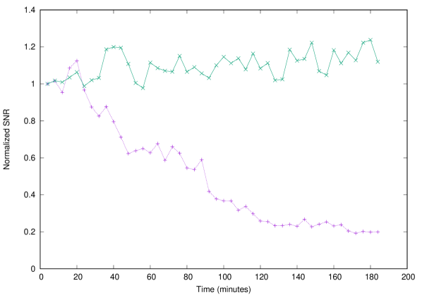
Figure 1: The variation of the normalized SNR with time for the case in which the array is phased only at the start of the observations (dotted line) as well as the case in which the array is re-phased every 4 min. (solid line) using phases derived from the measured visibilities and a model of the target field. The normalized SNR is computed over 4 min. intervals and normalized by the value of the SNR in the first 4 min.

For the observations with continuous infield phasing, a model image of the field was made using data from earlier observations and a CASA based imaging pipeline (Kudale & Chengalur, in preparation). Note that model generation was a one time operation, and the same model was used for all phasing cycles. The brightest source in the field had a flux of $\sim 80$ mJy, while the observed flux of the pulsar itself was $\sim 14$ mJy (these are the observed fluxes, i.e. without correction for the primary beam. Since the phasing is being done for the same telescope as the one from which the model was derived, it is the observed, and not the primary beam corrected flux that is of relevance). flagcal was run on a workstation with a 32 core intel processor running at 2.6 GHz with 256 GB of RAM. It takes about $\sim 60$ seconds to flag and calibrate $\sim 3$ minutes of data. We chose to compute and update the calibration solutions on a time scale of 4 min. The antenna based phase corrections determined by flagcal were uploaded to the correlator at the end of each 4 min. cycle. flagcal provides both amplitude and phase corrections for each antenna, however only the phases were updated. This is in keeping with the practise in conventional phasing, where only the phase derived from the phase calibrator is used to phase up the array. The phase update also correctly accounts for the fact that the phases determined by flagcal are an incremental correction over the phases that are currently loaded into the correlator. For the observations without continuous phasing, the phases were calculated (using the same model as for the observations with infield phasing) and applied only at the start of the observations.

The phased array data was de-dispersed using a dispersion measure of $73.782$ pc cm^-3 (i.e. the dispersion measure listed for PSR B0740-28 in the ATNF pulsar catalog (http://www.atnf.csiro.au/people/pulsar/psrcat/), and then each 4 min. time series was folded to obtain the average pulse profile over that time interval. We show in Fig. 1 the normalized SNR for the two observations. The normalized SNR is the observed SNR in a given 4 min. interval divided by the SNR for the first 4 min. interval. As can be seen in the case of infield phasing the SNR is maintained over a period of several hours, whereas in the absence of phasing the SNR rapidly degrades. In the next section we derive an general analytical expression for the time variation of the degradation of the SNR and compare it with the observed one.

3.1 Time variation of the SNR in the absence of continuous re-phasing

Because of drifts in the instrumental phase as well as changes in the ionospheric conditions, one would expect that in the absence of re-phasing the SNR of a phased array would gradually decrease with time. In Appendix A we derive from first principles the relative SNR expected for various different kinds of arrays, including phased arrays in which the phasing is not perfect. We show that under the assumption that (1) the self noise from the source is negligible and (2) the phase error on all baselines can be characterized as a Gaussian random variable with variance $\sigma^{2}$, the SNR for an N identical element array scales as

$$\frac{GS+(N-1)(GS)e^{-\sigma^{2}/2}}{({\rm T}_{\rm A}+{\rm T}_{\rm R})}$$ (4)

where T_R is the “receiver” temperature of the antenna (i.e. the noise contribution from the LNA and any other sources that are independent for different antennas) and T_A is the “antenna temperature”, i.e. the noise contribution from the sky and any other sources that are correlated between the different antennas.

In the case that we are interested in here, viz. that the antennas are initially phased, but slowly get dephased, the change in the phase with time can be characterized by the structure function

$$\sigma^{2}_{\phi}=<(\phi(t+\tau)-\phi(t))^{2}>$$ (5)

For Kolmogorov turbulence in the “frozen in” approximation, the structure function is given by $D(\tau)\sim\tau^{5/3}$ (thompson01, ). The signal to noise ratio will hence vary as

$${\rm SNR}(\tau)=\frac{(GS)+(N-1)(GS)e^{-(\tau/\tau_{0})^{5/3}}}{({\rm T}_{\rm A}+{\rm T}_{\rm R})}$$ (6)

where $\tau_{0}$ is some constant.

We have assumed above that variance of the phase is the same for all the baselines in the array. In general however, the phase variation is faster on the longer baselines (nice92, ). For an array like the GMRT which has about half of the antennas in a compact “central square” and the remainder in sparse extended “Y” shaped arms (swarup91, ), the central square antennas generally maintain their phase coherence for significantly longer than the arm antennas. If we make the simplifying assumption that over the observing interval some fraction of the antennas remain phased (i.e. $\sigma^{2}_{\phi}\approx 0$), while the phase drifts on the remaining antennas, the degradation in the SNR can then be generically approximated as

$${\rm SNR}(\tau)=\alpha+\beta e^{-(\tau/\tau_{0})^{5/3}}$$ (7)

The functional form given in Eqn. (7) was fit to the data in Fig. 1 without continuous infield phasing and the resulting best fit along with the original data are shown in Fig. 2. As can be seen the expression in Eqn. (7) gives an excellent fit to the data. The best fit values of the different parameters are $\alpha=0.18\pm 0.02,\beta=0.87\pm 0.03,\tau_{0}=82.1\pm 4.4$ minutes. In situations where either conventional phasing is done, or the time interval between two successive infield phasing cycles is large, Eqn. (7) allows one to estimate the degradation in SNR in the time interval between the phase updates. We note that, in general, $\alpha$, $\beta$ and $\tau_{0}$ would depend on the baseline length distribution in the array as well as the observing frequency. It would be interesting to try and determine the frequency dependence of these parameters using future GMRT observations.

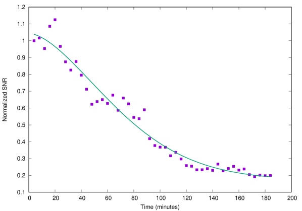
Figure 2: The variation of the SNR with time (solid points) in the case that phasing is done only at the start of the observation. The solid line shows the best fit function of the form ${\rm SNR}(\tau)=\alpha+\beta e^{-(\tau/\tau_{0})^{5/3}}$. See the text for more details.

4 Discussion and Conclusions

We presented a scheme for infield phasing for the GMRT where the visibility data obtained in parallel with the observations are used to phase up the voltages used to form the phased array beam. The primary requirement for such a scheme to work is that there is sufficient flux in the background continuum sources to allow for reliable calibration solutions to be found for integration times of the order of a few minutes. Experience at the GMRT indicates that this is generally the case in most fields at frequencies of 610 MHz or lower.

We also present (in the appendix) the expected SNR for different kinds of arrays, in particular for a phased array in which the phasing is not perfect. This allows us also to derive a generic expression for the degradation in the SNR as the antenna phases drift away from alignment due to ionospheric changes. We note that the dephasing not only degrades the SNR, but would also affect the phased array beam; phase errors would have the effect of broadening the synthesized beam. It is interesting to check if there is a trade off here – would introduction of a slight amount of dephasing (either on purpose, or indavertently) lead to a faster survey speed? Or does the decrease in signal to noise ratio out weigh the change in the field of view?

These questions are difficult to answer in general case where the phase variation is different on different baselines. However, as discussed above, it is generally the case that the phase errors increase with baseline length. In order to derive a simple analytical formula, we make the assumption that the phase errors are such that $\sigma_{\phi}^{2}(u,v)\sim 2a^{2}(u^{2}+v^{2})$ and further that the baseline density distribution is also Gaussian (i.e. $e^{-b^{2}(u^{2}+v^{2})}$). In this case both the degradation in the SNR and the increase in the synthesized beam size can be analytically computed. In the absence of phase errors, the synthesized beam (i.e. the image corresponding to a point source of unit flux at the phase centre) is given by

$$\int_{-\infty}^{\infty}\int_{-\infty}^{\infty}dudv\ e^{-b^{2}(u^{2}+v^{2})}e^{-i2\pi(ul+vm)}\sim e^{-\pi^{2}(l^{2}+m^{2})/b^{2}}$$ (8)

Where we have ignorned the normalization, and focussed only on the shape of the synthesized beam. The area covered at the half maximum level is clearly $\propto b^{2}$. In the presense of phase errors, the visbility on a baseline with separation (u,v) instead of being unity would be $e^{-\sigma_{\phi}^{2}(u,v)/2}$ (see Sec. A.2). The synthesized beam would then be given by

$$\int_{-\infty}^{\infty}\int_{-\infty}^{\infty}dudv\ e^{-a^{2}(u^{2}+v^{2})}e^{-b^{2}(u^{2}+v^{2})}e^{-i2\pi(ul+vm)}\sim e^{-\pi^{2}(l^{2}+m^{2})/(a^{2}+b^{2})}$$ (9)

for which the field of view at the half power level scales as $(a^{2}+b^{2})$. The field of view on dephasing hence increases by $\frac{a^{2}+b^{2}}{b^{2}}$. To get the degradation in the signal to noise ratio we need to compute the baseline weighted average of $e^{-\sigma_{\phi}^{2}(u,v)/2}$. This is given by

$$<e^{-\sigma_{\phi}^{2}}> = \frac{\int_{-\infty}^{\infty}\int_{-\infty}^{\infty}dudv\ e^{-(a^{2}+b^{2})(u^{2}+v^{2})}}{\int_{-\infty}^{\infty}\int_{-\infty}^{\infty}dudv\ e^{-b^{2}(u^{2}+v^{2})}}$$ (10)

$$= \frac{b^{2}}{a^{2}+b^{2}}$$ (11)

That is, the SNR degrades by the factor $b^{2}/(a^{2}+b^{2})$, which means that one would have to integrate longer by the square of this factor in order to reach the same SNR as that of a perfectly phased array. The ratio of survey speeds for the perfectly phased array to partially dephased array is hence $b^{2}/(a^{2}+b^{2})$, i.e. the partially dephased array has a slower survey speed than the perfectly phased one.

To summarize, we present data from pulsar observations done at the GMRT using infield phasing with phase corrections derived from the visibilities obtained towards the target field, and updated every 4 min. We find that, as expected, with this quasi-continuous phasing the sensitivity of the phased array can be sustained over long periods of time. In contrast, the sensitivity in the situation where the array is phased only at the start of the observations falls rapidly. We find that the drop in sensitivity is consistent with that expected for phase fluctuations caused by Kolmogorov type turbulence in the ionosphere. Infield phasing has the advantage of not only maintaining the sensitivity of the array, but also of (1) improving the observing efficiency (since one does not have to periodically slew to a calibrator source) and also, (2) for the same reason enabling long continuous data runs on a given target.

Appendix A APPENDIX: Array Signal to Noise Ratios

We derive here from first principles the degradation in the signal to noise ratio (SNR) for an imperfectly phased array. For completeness we present the derivation also for an incoherent array. The derivation has (as would be expected) similarities with the SNR for imaging arrays (thompson01, ; rohlfs96, ) but we briefly summarize all the steps in the derivation, so that this presentation stands by itself.

Consider an array of N identical antennas, with “receiver” temperature T_R  (defined more precisely below) and gain G (in units of K/Jy). That is an unresolved 1 Jy source at the centre of the primary beam produces an antenna temperature of G K. Let us assume that all of the antennas are observing a source of flux S that is located at the centre of primary beam of all the antennas which is also the phase centre of the observations. We further assume that the sky is empty apart from the source at the phase center. (We relax these requirements below). Since our primary aim is to compare the SNR in different scenarios , we ignore the effect of other parameters such as the bandwidth, integration time, number of polarisations, etc. which we will assume to be kept the same for all the situations that we discuss.

The voltage signal v_i from an individual element is given by ${\rm v}_{\rm i}={\rm s}_{\rm i}+{\rm e}_{\rm i}$, where s_i is the signal voltage and e_i is the noise voltage. We will assume that both of these have a zero mean Gaussian distribution. So $<{\rm s}_{\rm i}>=<{\rm e}_{\rm i}>=0$. Further since the signal and noise, as well as the noise from different antennas are independent, we have $<{\rm s}_{\rm i}{\rm e}_{\rm i}>=0$, and $<{\rm e}_{\rm i}{\rm e}_{\rm j}>=0$ for $i\neq j$. Here we are explicitly assuming that e_i contains no component that is correlated between antennas, i.e. arises entirely from the receiver noise, including ground pickup etc.(We discuss below the modifications that arise when these assumptions are relaxed). Under the assumptions listed above, we have $<{\rm s}_{\rm i}{\rm s}_{\rm j}^{*}>={\rm GS}$ and $<{\rm e}_{\rm i}{\rm e}_{\rm i}^{*}>={\rm T}_{\rm R}$.

A.1 Incoherent Arrays

The power p_i measured by antenna $i$ is given by ${\rm p}_{\rm i}={\rm v}_{\rm i}^{2}$. If the power from the incoherent array is $y$, we have

$$y=\sum\limits_{i=1}^{N}{\rm p}_{\rm i}$$

We hence have

$$<y>=\sum\limits_{i}<{\rm s}_{\rm i}^{2}+{\rm e}_{\rm i}^{*}{\rm s}_{\rm i}+{\rm s}_{\rm i}^{*}{\rm e}_{\rm i}+{\rm e}_{\rm i}^{2}>={\rm N(GS+{\rm T}_{\rm R})}$$ (12)

The “signal” part of this is NGS. In order to compute the “noise” part we need to compute the variance of $y$. As a first step we compute $<y^{2}>$. We have

$$<y^{2}> = <\sum\limits_{i}({\rm s}_{\rm i}+{\rm e}_{\rm i})^{2}\sum\limits_{j}({\rm s}_{\rm j}+{\rm e}_{\rm j})^{2}>$$ (13)

$$= <\sum\limits_{i}\sum\limits_{j}({\rm s}_{\rm i}+{\rm e}_{\rm i})({\rm s}_{\rm i}^{*}+{\rm e}_{\rm i}^{*})({\rm s}_{\rm j}+{\rm e}_{\rm j})({\rm s}_{\rm j}^{*}+{\rm e}_{\rm j}^{*})>$$ (14)

For a Gaussian distribution, the fourth moment can be written in terms of products of the second moment, (see e.g. shynk12 ) viz.

$$\begin{split}<({\rm s}_{\rm i}+{\rm e}_{\rm i})({\rm s}_{\rm i}^{*}+{\rm e}_{\rm i}^{*})({\rm s}_{\rm j}+{\rm e}_{\rm j})({\rm s}_{\rm j}^{*}+{\rm e}_{\rm j}^{*})>&=<({\rm s}_{\rm i}+{\rm e}_{\rm i})({\rm s}_{\rm i}^{*}+{\rm e}_{\rm i}^{*})><({\rm s}_{\rm j}+{\rm e}_{\rm j})({\rm s}_{\rm j}^{*}+{\rm e}_{\rm j}^{*})>\\ &+<({\rm s}_{\rm i}+{\rm e}_{\rm i})({\rm s}_{\rm j}+{\rm e}_{\rm j})><({\rm s}_{\rm i}^{*}+{\rm e}_{\rm i}^{*})({\rm s}_{\rm j}^{*}+{\rm e}_{\rm j}^{*})>\\ &+<({\rm s}_{\rm i}+{\rm e}_{\rm i})({\rm s}_{\rm j}^{*}+{\rm e}_{\rm j}^{*})><({\rm s}_{\rm i}^{*}+{\rm e}_{\rm i}^{*})({\rm s}_{\rm j}+{\rm e}_{\rm j})>\end{split}$$ (15)

The second term in the sum is zero. To evaluate the remaing two terms, let us consider two separate cases, one when $i=j$, and the other when $i\neq j$. When $i=j$, the sum evaluates to 2(GS +T_R)², and there are N such terms. A term with $i\neq j$ evaluates to $(GS)^{2}+(GS+{\rm T}_{\rm R})^{2}$ (where we have used the fact that ${\rm s}_{\rm i}={\rm s}_{\rm j}$, i.e. the sky signal is 100% correlated). There are N(N-1) terms with $i\neq j$. Putting all of this together we get

$$<y^{2}>=2N({\rm GS+{\rm T}_{\rm R}})^{2}+N(N-1)[({\rm GS+{\rm T}_{\rm R}})^{2}+({\rm GS})^{2}]$$ (16)

and hence

$$\sigma_{y}^{2}=<y^{2}>-<y>^{2}=N[({\rm GS+{\rm T}_{\rm R}})^{2}+(N-1)(GS)^{2}]$$ (17)

The signal to noise ratio for the incoherent array is hence

$${\rm SNR}=\frac{\sqrt{N}{\rm GS}}{[({\rm GS+{\rm T}_{\rm R}})^{2}+(N-1)({\rm GS})^{2}]^{1/2}}$$ (18)

Let us now relax the condition that there is only one source in the sky. To understand the situation where we have multiple sources (or wide spread diffuse emission) it is useful to first consider the situation where we still have only one source of flux S in the sky, except that it is not at the phase and pointing center. For the $i^{th}$ antenna let $\Delta\tau_{i}$ be the differential geometric delay between the phase center and the position of the source. It is assumed that all delay measurements are with respect to some reference position in the array, and the delays can hence be treated as being antenna based. If s_i is the signal voltage at the $i^{th}$ antenna, we then have $<{\rm s}_{\rm i}{\rm s}_{\rm i}^{*}>=\rm G^{{}^{\prime}}S$, where $\rm G^{{}^{\prime}}$ is the gain in the direction of the source. Further

$$<{\rm s}_{\rm i}{\rm s}_{\rm j}^{*}>=\rm G^{{}^{\prime}}Se^{-i2\pi\nu\Delta\tau_{ij}}$$ (19)

where $\Delta\tau_{ij}=\Delta\tau_{i}-\Delta\tau_{j}$. Clearly, $<{\rm s}_{\rm j}{\rm s}_{\rm i}^{*}>=\rm G^{{}^{\prime}}Se^{i2\pi\nu\Delta\tau_{ij}}$. Using these relations to compute $<y>$ and $<y^{2}>$ as above, we find that the non zero phase terms cancel out and the only change is that G is to be replaced by $\rm G^{{}^{\prime}}$. This is again understandable, since we are dealing with the power from each antenna, and the signal phase clearly cannot make a difference to the total power. One assumption that we have made is that the bandwidth and the integration time are such that time and bandwidth smearing effects can be ignored, which is a reasonable assumption for sources within the main beam of the individual antennas. For a collection of point sources, the power from each source is additive, so if we have multiple point sources in the sky, Eqn. (18) continues to hold, except that the term GS in the denominator has to be replaced by T_A, the antenna temperature. Similarly diffuse emission can be regarded as emission from a collection of point sources distributed uniformly across the sky, and so once again Eqn. (18) applies with GS replaced by T_A. In general therefore, the signal to noise ratio of an incoherent array becomes

$${\rm SNR}=\frac{\sqrt{N}{\rm GS}}{[({\rm{\rm T}_{\rm A}+{\rm T}_{\rm R}})^{2}+(N-1){\rm T}_{\rm A}^{2}]^{1/2}}$$ (20)

Clearly in situations where the sky noise is negligible the SNR will improve as $\sqrt{N}$; in the opposite extreme when the total noise is sky dominated, the SNR is independent of $N$ for large $N$. An plot of the increase in the SNR with N for different values of ${\rm T}_{\rm A}/{\rm T}_{\rm R}$ is shown in Fig. 3. As can be seen in situations where T_A is a reasonable fraction of T_R one quickly reaches a stage where the SNR saturates and there is diminishing returns from adding further antennas into the array. In such situations, surveys would benefit from using a “fly’s eye” mode of observation with sub-arrays (i.e. where different sub-arrays look at different regions of the sky) instead of adding further antennas into the array.

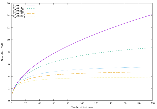
Figure 3: The variation of the SNR of an incoherent array as a function of the number of elements $N$. The solid line shows the ideal case where the SNR increases as $\sqrt{N}$ (which requires ${\rm T}_{\rm A}=0$), the thick dashed line is for ${\rm T}_{\rm A}=0.1{\rm T}_{\rm R}$ (which roughly corresponds to the GMRT 610 MHz band), the thin dashed line for ${\rm T}_{\rm A}=0.2{\rm T}_{\rm R}$, the bold dashed dot line for ${\rm T}_{\rm A}=0.25{\rm T}_{\rm R}$, and the thin dashed dot line is for ${\rm T}_{\rm A}=0.33{\rm T}_{\rm R}$ (which roughly corresponds to the expected value for SKA-mid (dewdney13, ). As discussed in the text, for arrays with large number of elements, a “fly’s eye” mode of observation with sub-arrays would be a more efficient survey mode than using all of the antennas in the array to form a single incoherent array.

A.2 Phased Arrays

Let us again start with the scenario where the array is observing an unresolved source of flux S which is at the phase and pointing center. Let us further assume that the antenna temperature (due to all the sources including diffuse emission) is T_A, but that this emission is completely resolved out on all baselines (i.e. when summed over all the sources in the field of view the phase term in Eqn. (19) averages out to zero). Then the only correlation between the voltages at different antennas is that arising from the source at the phase centre.

Let ${\rm v}_{\rm i}={\rm s}_{\rm i}+{\rm e}_{\rm i}$ be the voltage from the $i^{th}$ antenna. We assume that the phase difference $\phi_{ij}$ between the signals from the $i^{th}$ and $j^{th}$ antenna has a Gaussian distribution with zero mean and variance $\sigma^{2}$. Then $<{\rm v}_{\rm i}{\rm v}_{\rm j}^{*}>=GS<e^{i\phi_{ij}}>=GSe^{-\sigma^{2}/2}$, ($i\neq j$), and $<{\rm v}_{\rm i}{\rm v}_{\rm i}^{*}>={\rm T}_{\rm A}+{\rm T}_{\rm R}$. For simplicity we assumed that the phase variance $\sigma^{2}$ is the same for all baselines. Let the total power output of the phased array be $y$, i.e. $y=(\sum\limits_{i}{\rm s}_{\rm i}+{\rm e}_{\rm i})^{2}$. The expected value of $y$ is then given by

$$<y> = <\sum\limits_{i}({\rm s}_{\rm i}+{\rm e}_{\rm i})\sum\limits_{j}({\rm s}_{\rm j}^{*}+{\rm e}_{\rm j}^{*})>$$ (21)

$$= \sum\limits_{i,j}<{\rm s}_{\rm i}{\rm s}_{\rm j}^{*}>+<{\rm e}_{\rm i}{\rm e}_{\rm j}^{*}>$$ (22)

$$= N({\rm T}_{\rm A}+{\rm T}_{\rm R})+N(N-1)GSe^{-\sigma^{2}/2}$$ (23)

where we have used the fact that in the summation there are N terms with $i=j$ (i.e. auto-correlations), and N(N-1) terms with $i\neq j$ (i.e. cross-correlations, which are also called “visibilities” in the imaging context).

As before, in order to estimate the variance of $y$ let us first compute $<y^{2}>$. We have

$$<y^{2}>=<\sum\limits_{i}({\rm s}_{\rm i}+{\rm e}_{\rm i})\sum\limits_{j}({\rm s}_{\rm j}^{*}+{\rm e}_{\rm j}^{*})\sum\limits_{k}({\rm s}_{\rm k}+{\rm e}_{\rm k})\sum\limits_{l}({\rm s}_{\rm l}^{*}+{\rm e}_{\rm l}^{*})>$$ (25)

Again, as before this $4^{th}$ moment can be written as a product of second moments and evaluated. We omit the calculation and only give the final result, which is

$$<y^{2}>=2N^{2}({\rm T}_{\rm A}+{\rm T}_{\rm R})^{2}+4N^{2}(N-1)(GS)({\rm T}_{\rm A}+{\rm T}_{\rm R})e^{-\sigma^{2}/2}+2N^{2}(N-1)^{2}(GS)^{2}e^{-\sigma^{2}}$$ (26)

From Eqns. (26) and (LABEL:eqn:ych) we get the variance of $y$ to be

$$\sigma^{2}_{y}=N^{2}({\rm T}_{\rm A}+{\rm T}_{\rm R})^{2}+2N^{2}(N-1)(GS)({\rm T}_{\rm A}+{\rm T}_{\rm R})e^{-\sigma^{2}/2}+N^{2}(N-1)^{2}(GS)^{2}e^{-\sigma^{2}}$$ (27)

and hence the signal to noise ratio is

$$\frac{GS+(N-1)(GS)e^{-\sigma^{2}/2}}{[({\rm T}_{\rm A}+{\rm T}_{\rm R})^{2}+(N-1)(GS)({\rm T}_{\rm A}+{\rm T}_{\rm R})e^{-\sigma^{2}/2}+(N-1)^{2}(GS)^{2}e^{-\sigma^{2}}]^{1/2}}$$ (28)

It is worth high lighting a couple of limiting cases of Eqn. (28). In the case where the phasing is perfect (i.e. $\sigma\to 0$) we have

$${\rm SNR}=\frac{N({\rm GS})}{[({\rm T}_{\rm A}+{\rm T}_{\rm R})^{2}+(N-1)(GS)({\rm T}_{\rm A}+{\rm T}_{\rm R})+(N-1)^{2}(GS)^{2}]^{1/2}}$$ (29)

which reduces to N(GS)/(T_A+T_R) in the case that ${\rm GS}<<({\rm T}_{\rm A}+{\rm T}_{\rm R})$. Note that this expression holds even if ${\rm T}_{\rm A}>>{\rm T}_{\rm R}$. In the case that ${\rm T}_{\rm A}<<{\rm T}_{\rm R}$, the SNR of the phased array is $\sqrt{(}N)$ times better than that of an incoherent array. In the other extreme (i.e. when (${\rm T}_{\rm A}>>{\rm T}_{\rm R}$) and for large $N$, the SNR of the phased array is $N$ times better than that of the incoherent array. On the other hand when the phase is completely random, (i.e. is uniformly distributed over [$0,2\pi$]), then $<{\rm s}_{\rm i},{\rm s}_{\rm j}^{*}>$ =0, then the signal to noise ratio reduces to (GS)/(T_A+T_R) = GS/T_S), i.e. the same as for a single dish. Essentially, in this case, both the signal as well as the noise increase identically (since the signal is not phased up) when one combines together the voltages from different antennas. In such a situation, the SNR of a “phased” array would in fact be worse than that of an incoherent array.

Figure 4: The variation of the normalized SNR for a phased array as a function of the number of elements $N$. The normalized SNR is the SNR divided by the SNR for a single antenna. The solid line shows the ideal case where the SNR increases as $N$ (which requires the source flux to be negligible, and the phase error to be $0$), the thick dashed line is for a negligible source flux and phase rms of $0.3$ radians, the thin dashed line for $GS/{\rm T}_{\rm S}=2.5\times 10^{-4}$ (which roughly corresponds to observation of a 100 mJy source with the SKA-mid, (dewdney13, ))and a phase rms of $0.0$, the bold dashed dot line for $GS/{\rm T}_{\rm S}=2.5\times 10^{-3}$ and a phase rms of $0.0$, and the thin dashed dot line is for $GS/{\rm T}_{\rm S}=2.5\times 10^{-3}$ and a phase rms of $0.3$ rad. As discussed in the text in the limiting case where the antenna phases are uniformly distributed over [$0,2\pi$], the SNR does not increase with increasing the number of antennas in the array.

A.3 Post Correlation Beam Formation

When forming the coherent phased array beam we assumed that the antenna voltages were added together and then squared, in order to get the phased array beam. In an interferometric array one could also produce the phased array beam from the visibilities produced by the correlator, a technique sometimes called “post-correlation beamforming”. If we exclude the N auto-correlations, then, from Eqn. (LABEL:eqn:ych) the mean value of the power in the post-correlation beam is $N(N-1)GSe^{-\sigma^{2}/2}$. Although this is smaller than the corresponding number for the phased array beam, it does not contain terms proportional to the receiver temperature T_R  and is hence likely to be less subject to systematic variations produced by fluctuations in the receiver power, ground pick up etc. Following similar arguments as given above for the phased array, the signal to noise ratio for post-correlation beam can be shown to be

$$\frac{(\sqrt{N(N-1)}(GS)e^{-\sigma^{2}/2}}{[({\rm T}_{\rm A}+{\rm T}_{\rm R})^{2}+2(N-2)(GS)({\rm T}_{\rm A}+{\rm T}_{\rm R})e^{-\sigma^{2}/2}+((N-1)(N-2)+1)(GS)^{2}e^{-\sigma^{2}}]^{1/2}}$$ (30)

which in the limit of small $S$ is $\sqrt{N(N-1)}/N$ times smaller than that of the conventional phased array. This is a small factor for large N.

A.4 Incoherent Combination of Phased Arrays

We could also consider the situation (which occurs for example in the LOFAR array, haarlem13 ) where we have two levels of array formation. First an coherent array is formed from a cluster of nearby elements (a “station”) and then an incoherent array is formed from these stations. If there are N elements (each of gain G) in a station, and M such stations, then the expected value of the total power is $MN({\rm T}_{\rm A}+{\rm T}_{\rm R})+MN^{2}GS$. We have assumed that (1) all the elements in a station are perfectly phased, and (2) that the diffuse sky emission is dominant and (3) that the power in the cross-correlation between the elements in a station is small compared to the power in the auto-correlations (i.e. the terms involving $e^{-\sigma^{2}}$ and $e^{-\sigma^{2}/2}$ in eqn.( 28) can be ignored). Essentially we are assuming that the diffuse emission is mostly resolved out on the baselines between the elements in a station. We note that this is an extreme assumption, and that in real life arrays, while the cross-correlation power is less than the auto-correlation power, it may not be so small as to be neglected altogether.

For the variance in the final signal formed by incoherently combining the powers of the stations we will have to compute

$$<y^{2}>=<\sum\limits_{m=1}^{M}\sum\limits_{n=1}^{M}\sum\limits_{j=1}^{N}\sum\limits_{j=1}^{N}\sum\limits_{k=1}^{N}\sum\limits_{l=1}^{N}<v_{mi}v_{mj}^{*}v_{nk}v_{nl}^{*}>$$ (31)

Since we have assumed that diffuse emission dominates, and that it is resolved out on the baselines between the elements in a station, it follows that it would also be resolved out on the baselines between the elements in different stations. So in the summation above, one set of terms which contribute are those with $n=m$, i.e. the elements within a given station. This contribution is given by $2N^{2}({\rm T}_{\rm A}+{\rm T}_{\rm R})^{2}$. There will be $M$ such terms. For $n\neq m$, the only terms in the $4^{th}$ moment that will contribute are of the form $<v_{mi}v_{mi}^{*}><v_{nk}v_{nk}^{*}>$. There are $M(M-1)N^{2}$ such terms, each of which evaluates to $({\rm T}_{\rm A}+{\rm T}_{\rm R})^{2}$. We hence have

$$\sigma_{y}^{2} = M(M-1)N^{2}({\rm T}_{\rm A}+{\rm T}_{\rm R})^{2}+2MN^{2}({\rm T}_{\rm A}+{\rm T}_{\rm R})^{2}-M^{2}N^{2}({\rm T}_{\rm A}+{\rm T}_{\rm R})^{2}$$ (32)

$$= MN^{2}({\rm T}_{\rm A}+{\rm T}_{\rm R})^{2}$$ (33)

The signal to noise ratio is hence

$${\rm SNR}=\frac{\sqrt{M}N(GS)}{({\rm T}_{\rm A}+{\rm T}_{\rm R})}$$ (35)

that is, it increases as $\sqrt{M}$ (i.e. the square root of the number of stations), even though the noise on the individual elements is sky dominated (i.e. ${\rm T}_{\rm A}>{\rm T}_{\rm R}$).

- (1) D.J. Nice, S.E. Thorsett, ApJ 397, 249 (1992). DOI 10.1086/171784
- (2) J. van Leeuwen, B.W. Stappers, A&A 509, A7 (2010). DOI 10.1051/0004-6361/200913121
- (3) B. Bhattacharyya, Y. Gupta, J. Gil, MNRAS 383, 1538 (2008). DOI 10.1111/j.1365-2966.2007.12666.x
- (4) J. Roy, Y. Gupta, U.L. Pen, J.B. Peterson, S. Kudale, J. Kodilkar, Experimental Astronomy 28, 25 (2010). DOI 10.1007/s10686-010-9187-0
- (5) F.R. Schwab, in 1980 International Optical Computing Conference I, Proc. of the SPIE, vol. 231, ed. by W.T. Rhodes (1980), Proc. of the SPIE, vol. 231, pp. 18–25. DOI 10.1117/12.958828
- (6) T.J. Cornwell, P.N. Wilkinson, MNRAS 196, 1067 (1981). DOI 10.1093/mnras/196.4.1067
- (7) T. Cornwell, E.B. Fomalont, in Synthesis Imaging in Radio Astronomy, Astronomical Society of the Pacific Conference Series, vol. 6, ed. by R.A. Perley, F.R. Schwab, A.H. Bridle (1989), Astronomical Society of the Pacific Conference Series, vol. 6, p. 185
- (8) A.R. Thompson, J.M. Moran, G.W.J. Swenson, Interferometry and Synthesis in Radio Astronomy, 2nd edn. (Wiley Interscience, 2001)
- (9) J. Prasad, J. Chengalur, Experimental Astronomy 33, 157 (2012). DOI 10.1007/s10686-011-9279-5
- (10) J.N. Chengalur, FLAGCAL: a flagging and calibration pipeline for GMRT DATA. Tech. Rep. NCRA/COM/001, NCRA-TIFR (2013)
- (11) G. Swarup, S. Ananthakrishnan, V.K. Kapahi, A.P. Rao, C.R. Subrahmanya, V.K. Kulkarni, Current Science, Vol. 60, NO.2/JAN25, P. 95, 1991 60, 95 (1991)
- (12) K. Rohlfs, T.L. Wilson, Tools of Radio Astronomy, 2nd edn. (Springer, 1996)
- (13) J.Y. Shynk, Probability, Random Variables and Random Processes: Theory and Signal Processing Applications (Wiley-Interscience, 2012)
- (14) P.E. Dewdney, SKA1 System Baseline Design. Tech. Rep. SKA-TEL-SKO-DD-001, SKA Office (2013)
- (15) M.P. van Haarlem, M.W. Wise, A.W. Gunst, G. Heald, J.P. McKean, J.W.T. Hessels, A.G. de Bruyn, R. Nijboer, J. Swinbank, R. Fallows, M. Brentjens, A. Nelles, R. Beck, H. Falcke, R. Fender, J. Hörandel, L.V.E. Koopmans, G. Mann, G. Miley, H. Röttgering, B.W. Stappers, R.A.M.J. Wijers, S. Zaroubi, M. van den Akker, A. Alexov, J. Anderson, K. Anderson, A. van Ardenne, M. Arts, A. Asgekar, I.M. Avruch, F. Batejat, L. Bähren, M.E. Bell, M.R. Bell, I. van Bemmel, P. Bennema, M.J. Bentum, G. Bernardi, P. Best, L. Bîrzan, A. Bonafede, A.J. Boonstra, R. Braun, J. Bregman, F. Breitling, R.H. van de Brink, J. Broderick, P.C. Broekema, W.N. Brouw, M. Brüggen, H.R. Butcher, W. van Cappellen, B. Ciardi, T. Coenen, J. Conway, A. Coolen, A. Corstanje, S. Damstra, O. Davies, A.T. Deller, R.J. Dettmar, G. van Diepen, K. Dijkstra, P. Donker, A. Doorduin, J. Dromer, M. Drost, A. van Duin, J. Eislöffel, J. van Enst, C. Ferrari, W. Frieswijk, H. Gankema, M.A. Garrett, F. de Gasperin, M. Gerbers, E. de Geus, J.M. Grießmeier, T. Grit, P. Gruppen, J.P. Hamaker, T. Hassall, M. Hoeft, H.A. Holties, A. Horneffer, A. van der Horst, A. van Houwelingen, A. Huijgen, M. Iacobelli, H. Intema, N. Jackson, V. Jelic, A. de Jong, E. Juette, D. Kant, A. Karastergiou, A. Koers, H. Kollen, V.I. Kondratiev, E. Kooistra, Y. Koopman, A. Koster, M. Kuniyoshi, M. Kramer, G. Kuper, P. Lambropoulos, C. Law, J. van Leeuwen, J. Lemaitre, M. Loose, P. Maat, G. Macario, S. Markoff, J. Masters, R.A. McFadden, D. McKay-Bukowski, H. Meijering, H. Meulman, M. Mevius, E. Middelberg, R. Millenaar, J.C.A. Miller-Jones, R.N. Mohan, J.D. Mol, J. Morawietz, R. Morganti, D.D. Mulcahy, E. Mulder, H. Munk, L. Nieuwenhuis, R. van Nieuwpoort, J.E. Noordam, M. Norden, A. Noutsos, A.R. Offringa, H. Olofsson, A. Omar, E. Orrú, R. Overeem, H. Paas, M. Pandey-Pommier, V.N. Pandey, R. Pizzo, A. Polatidis, D. Rafferty, S. Rawlings, W. Reich, J.P. de Reijer, J. Reitsma, G.A. Renting, P. Riemers, E. Rol, J.W. Romein, J. Roosjen, M. Ruiter, A. Scaife, K. van der Schaaf, B. Scheers, P. Schellart, A. Schoenmakers, G. Schoonderbeek, M. Serylak, A. Shulevski, J. Sluman, O. Smirnov, C. Sobey, H. Spreeuw, M. Steinmetz, C.G.M. Sterks, H.J. Stiepel, K. Stuurwold, M. Tagger, Y. Tang, C. Tasse, I. Thomas, S. Thoudam, M.C. Toribio, B. van der Tol, O. Usov, M. van Veelen, A.J. van der Veen, S. ter Veen, J.P.W. Verbiest, R. Vermeulen, N. Vermaas, C. Vocks, C. Vogt, M. de Vos, E. van der Wal, R. van Weeren, H. Weggemans, P. Weltevrede, S. White, S.J. Wijnholds, T. Wilhelmsson, O. Wucknitz, S. Yatawatta, P. Zarka, A. Zensus, J. van Zwieten, A&A 556, A2 (2013). DOI 10.1051/0004-6361/201220873