An economic approach to vehicle dispatching for ride sharing

Abstract

Over the past few years, ride-sharing has emerged as an effective way to relieve traffic congestion. A key problem for these platforms is to come up with a revenue-optimal (or GMV-optimal) pricing scheme and an induced vehicle dispatching policy that incorporate geographic and temporal information. In this paper, we aim to tackle this problem via an economic approach.

Modeled naively, the underlying optimization problem may be non-convex and thus hard to compute. To this end, we use a so-called “ironing” technique to convert the problem into an equivalent convex optimization one via a clean Markov decision process (MDP) formulation, where the states are the driver distributions and the decision variables are the prices for each pair of locations. Our main finding is an efficient algorithm that computes the exact revenue-optimal (or GMV-optimal) randomized pricing schemes. We characterize the optimal solution of the MDP by a primal-dual analysis of a corresponding convex program. We also conduct empirical evaluations of our solution through real data of a major ride-sharing platform and show its advantages over fixed pricing schemes as well as several prevalent surge-based pricing schemes.

1 Introduction

The recently established applications of shared mobility, such as ride-sharing, bike-sharing, and car-sharing, have been proven to be an effective way to utilize redundant transportation resources and to optimize social efficiency (Cramer and Krueger, 2016). Over the past few years, intensive researches have been done on topics related to the economic aspects of shared mobility (Crawford and Meng, 2011; Kostiuk, 1990; Oettinger, 1999).

Despite these researches, the problem of how to design revenue optimal prices and vehicle dispatching schemes has been largely open and one of the main research agendas in sharing economics. There are at least two challenges when one wants to tackle this problem in the real-world applications. First of all, due to the nature of transportation, the price and dispatch scheme must be geographically dependent. Secondly, the price and dispatch scheme must take into consideration the fact that supplies and demands in these environments may change over time. As a result, it may be difficult to compute, or even to represent a price and dispatch scheme for such complex environments.

Traditional price and dispatch schemes for taxis (Laporte, 1992; Gendreau et al., 1994; Ghiani et al., 2003) and airplanes (Gale and Holmes, 1993; Stavins, 2001; McAfee and Te Velde, 2006) do not capture the dynamic aspects of the environments: taxi fees are normally calculated by a fixed rate of distance and time and the prices of flight tickets are sold via relatively long booking periods, while in contrast, the customers of shared vehicles make their decisions instantly.

The dynamic ride-sharing market studied in this paper is also known to have imbalanced supply and demand, either globally in a city or locally in a particular time and location. Such imbalance in supply and demand is known to cause severe consequences on revenues (e.g, the so-called wild goose chase phenomenon (Castillo et al., 2017)). Surging price is a way to balance dynamic supply and demand (Chen and Sheldon, 2015) but there is no known guarantee that surge based pricing can dispatch vehicles efficiently and solve the imbalanced supplies and demands. Traditional dispatch schemes (Laporte, 1992; Gendreau et al., 1994; Ghiani et al., 2003) focus more on the algorithmic aspect of static vehicle routing, without consider pricing. However, vehicle dispatching and pricing problem are tightly related, since a new price scheme will surely induces a change on supply and demand since the drivers and passengers are strategic. In this paper, we aim to come up with price schemes with desirable induced supplies and demands.

1.1 Our contribution

In this paper, we propose a graph model to analyze the vehicle pricing and dispatching problem mentioned above. In the graph, each node refers to a region in the city and each edge refers to a possible trip that includes a pair of origin and destination as well as a cost associated with the trip on this edge. The design problem is, for the platform, to set a price and specify the vehicle dispatch for each edge at each time step. Drivers are considered to be non-strategic in our model, meaning that they will accept whatever offer assigned to them. The objective of the platform can either be its revenue or the GMV or any convex combination between them.

Our model naturally induces a Markov Decision Process (MDP) with the driver distributions on each node as states, the price and dispatch along each edge as actions, and the revenue as immediately reward. Although the corresponding mathematical program is not convex (thus computationally hard to compute) in general, we show that it can be reduced to a convex one without loss of generality. In particular, in the resulting convex program where the throughput along each source and destination pair in each time period are the variables, all the constraints are linear and hence the exact optimal solutions can be efficiently computed (Theorem 3.1).

We further characterize the optimal solution via primal-dual analysis. In particular, a pricing scheme is optimal if and only if the marginal contribution of the throughput along each edge equals to the system-wise marginal contribution of additional supply minus the difference of the long term contributions of unit supply at the origin and the destination (see Section 5).

We also perform extensive empirical analysis based on a public dataset with more than $8.5$ million orders. We compare our policy with other intensively studied policies such as surge pricing (Chen and Sheldon, 2015; Cachon et al., 2016; Castillo et al., 2017). Our simulations show that, in both the static and the dynamic environment, our optimal pricing and dispatching scheme outperforms surge pricing by $17\%$ and $33\%$. Interestingly, our simulations show that our optimal policy has much stronger ability in dispatching the vehicles than other policies, which results directly in its performance boost (see Section 6).

1.2 Related work

Driven by real-life applications, a large number of researches have been done on ride-share markets. Some of them employ queuing networks to model the markets (Iglesias et al., 2016; Banerjee et al., 2015; Tang et al., 2016). Iglesias et al. (2016) describe the market as a closed, multi-class BCMP queuing network which captures the randomness of customer arrivals. They assume that the number of customers is fixed, since customers only change their locations but don’t leave the network. In contrast, the number of customer are dynamic in our model and we only consider the one who asks for a ride (or sends a request to the platform). Banerjee et al. (2015) also use a queuing theoretic approach to analyze the ride-share markets and mainly focus on the behaviors of drivers and customers. They assume that the drivers enter or leave the market with certain possibilities. Bimpikis et al. (2016) take account for the spatial dimension of pricing schemes in ride-share markets. They price for each region and their goal is to rebalance the supply and demand of the whole market. However, we price for each routing and aim to maximize the total revenue or social welfare of the platform. We also refer the readers to the line of researches initiated by (Ma et al., 2013) for the problems about the car-pooling in the ride-sharing systems (Alonso-Mora et al., 2017; Zhao et al., 2014; Chan and Shaheen, 2012).

Many works on ride-sharing consider both the customers and the drivers to be strategic, where the drivers may reject the requests or leave the system if the prices are too low (Banerjee et al., 2015; Fang et al., 2017). As we mentioned, if the revenue sharing ratios between the platform and the drivers can be dynamic, then the pricing problem and the revenue sharing problem could be independent and hence the drivers are non-strategic in the pricing problem. In addition, the platform can also increase the profit by adopting dynamic revenue sharing schemes (Balseiro et al., 2017).

Another work closely related to ours is by Banerjee et al. (2017). Their work is concurrent and has been developed independently from ours. In particular, the customers arrive according to a queuing model and their pricing policy is state-independent and depends on the transition volume. Both their and our models are built upon the underlying Markovian transitions between the states (the distribution of drivers over the graph). The major differences are: (i) our model is built for the dynamic environments with a very large number of customers (each of them is non-atomic) to meet the practical situations, while theirs adopts discrete agent settings; (ii) they overcome the non-convexity of the problem by relaxation and focus only on concave objectives, which makes this work hard to use for real applications, while we solve the problem via randomized pricing and transform the problem to a convex program; (iii) they prove approximation bounds of the relaxation problem, while we give exact optimal solutions of the problem by efficiently solving the convex program.

2 Model

A passenger (she) enters the ride-sharing platform and sends a request including her origin and destination to the platform. The platform receives the request and determines a price for it. If user accepts the price, then the platform may decide whether to send a driver (he) to pick her up. The platform is also able to dispatch drivers from one place to another even there is no request to be served. By the pricing and dispatching methods above, the goal of maximizing revenue or social welfare of the entire platform can be achieved. Our model incorporates the two methods into a simple pricing problem. In this section, we define basic components of our model and consider two settings: dynamic environments with a finite time horizon and static environments with an infinite time horizon. Finally we reduce the action space of the problem and give a simple formulation.

Requests

We use a strongly connected digraph $G=(V,E)$ to model the geographical information of a city. Passengers can only take rides from nodes to nodes on the graph. When a passenger enters the platform, she expects to get a ride from node $s$ to node $t$, and is willing to pay at most $x\geq 0$ for the ride. She then sends to the platform a request, which is associated with the tuple $e=(s,t)$. Upon receiving the request, The platform sets a price $p$ for it. If the price is accepted by the passenger (i.e., $x\geq p$), then the platform tries to send a driver to pick her up. We say that the platform rejects the request, if no driver is available.

A request is said to be accepted if both the passenger accepts the price $p$ and there are available drivers. Otherwise, the request is considered to end immediately.

Drivers

Clearly, within each time period, the total number of accepted requests starting from $s$ cannot be more than the number of drivers available at $s$. Formally, let $q(e)$ denote the total number of accepted request along edge $e$, then:

$$\displaystyle\sum_{e\in\mathrm{OUT}(v)}q(e)\leq w(v),{~{}}\forall v\in V,$$ (2.1)

where $\mathrm{OUT}(v)$ is the set of edges starting from $v$ and $w(v)$ is the number of currently available drivers at node $v$.

In particular, we assume that both the total number of drivers and the number of requests are very large, which is often the case in practice, and consider each driver and each request to be non-atomic. For simplicity, we normalize the total amount of drivers on the graph to be $1$, thus $w(v)$ is a real number in $[0,1]$. We also normalize the number of requests on each edge with the total number of drivers. Note that the amount of requests on an edge $e$ can be more than $1$, if there are more requests on $e$ than the total drivers on the graph.

Geographic Status

For each accepted request on edge $e$, the platform will have to cover a transportation cost $c_{\tau}(e)$ for the driver. In the meanwhile, the assigned driver, who currently at node $s$, will not be available until he arrives the destination $t$. Let $\Delta\tau(e)$ be the traveling time from $s$ to $t$ and $\tau$ be the timestep of the driver leaving $s$. He will be available again at timestep $\tau+\Delta\tau(e)$ on node $t$. Formally, the amount of available drivers on any $v\in V$ is evolving according to the following equations:

$$w_{\tau+1}(v)=w_{\tau}(v)-\sum_{e\in\mathrm{OUT}(v)}q_{\tau}(e)+\sum_{e\in\mathrm{IN}(v)}q_{\tau+1-\Delta\tau(e)}(e),$$ (2.2)

where $\mathrm{IN}(v)$ is the set of edges ending at $v$. Here we add subscripts to emphasize the timestamp for each quantity. In particular, throughout this paper, we focus on the discrete time step setting, i.e., $\tau\in\mathbb{N}$.

Demand Function

As we mentioned, the platform could set different prices for the requests. Such prices may vary with the request edge $e$, time step $t$, and the driver distribution but must be independent of the passenger’s private value $x$ as it is not observable. Formally, let $D_{\tau}(\cdot|e):\mathbb{R}_{+}\rightarrow\mathbb{R}_{+}$ be the demand function of edge $e$, i.e., $D_{\tau}(p|e)$ is the amount of requests on edge $e$ with private value $x\geq p$ in time step $\tau$. Then the amount of accepted requests $q_{\tau}(e)\leq\operatorname*{\mathbb{E}}[D_{\tau}(p_{\tau}(e)|e)]$, where the expectation is taken over the potential randomness of the pricing rule $p_{\tau}(e)$.

Design Objectives

In this paper, we consider a class of state-irrelevant objective functions. A function is state-irrelevant if its value only depends on the amount of accepted request on each edge $q(e)$ but not the driver distribution of the system $w(v)$. Note that a wide range of objectives are included in our class of objectives, such as the revenue of the platform:

$$\mathrm{REVENUE}(p,q)=\sum_{e,\tau}\operatorname*{\mathbb{E}}[(p_{\tau}(e)-c_{\tau}(e))\cdot q_{\tau}(e)],$$

and the social welfare of the entire system:

$$\mathrm{WELFARE}(p,q)=\sum_{e,\tau}\operatorname*{\mathbb{E}}[(x-c_{\tau}(e))\cdot q_{\tau}(e)].$$

In general, our techniques work for any state-irrelevant objectives. Let $g(p,q)$ denote the general objective function and the dispatching and pricing problem can be formulated as follows:

maximize $$\displaystyle\sum_{e,\tau}g(p_{\tau}(e),q_{\tau}(e)|e)$$ (2.3)

subject to $$\hyperref@@ii[eq:feasible]{(\ref*{eq:feasible})}~{}\text{and}~{}\hyperref@@ii[eq:trans]{(\ref*{eq:trans})}.$$

Static and Dynamic Environment

In general, our model is defined for a dynamic environment in the sense that the demand function $D^{\tau}$ and the transportation cost $c_{\tau}$ could be different for each time step $\tau$. In particular, we study the problem (2.3) in general dynamic environments with finite time horizon from $\tau=1$ to $T$, where the initial driver distribution $w_{1}(v)$ is given as input.

In addition, we also study the special case with static environment and infinite time horizon, where $D^{\tau}\equiv D$ and $c_{\tau}\equiv c$ are consistent across each time step.

2.1 Reducing the action space

In this section, we rewrite the problem to an equivalent reduced form by incorporating the action of dispatching into pricing, i.e., using $p$ to express $q$. The idea is straightforward: (i) for the requests rejected by the platform, the platform could equivalently set an infinitely large price; (ii) if the platform is dispatching available drivers (without requests) from node $s$ to $t$, we can create virtual requests from $s$ to $t$ with $0$ value and let the platform sets price $0$ for these virtual requests. In fact, we can assume without loss of generality that $D(0|e)\equiv 1$, the total amount of drivers, because one can always add enough virtual requests for the edges with maximum demand less than $1$ or remove the requests with low values for the edges with maximum demand exceeds the total driver supply, $1$.

As a result, we may conclude that $q(e)\leq D(p|e)$. Since our goal is to maximize the objective $g(p,q)$, raising prices to achieve the same amount of flow $q(e)$ (such that $\operatorname*{\mathbb{E}}[D(p|e)]=q(e)$) never eliminates the optimal solution. In other words,

Observation .

The original problem is equivalent to the following reduced problem, where the flow variables $q_{\tau}(e)$ are uniquely determined by the price variables $p_{\tau}(e)$:

maximize $$\sum_{e,\tau}g(p_{\tau}(e),D_{\tau}(p_{\tau}(e)|e))$$ (2.4)

subject to $$q_{\tau}(e)=\operatorname*{\mathbb{E}}[D(p_{\tau}(e)|e)]$$

$$\hyperref@@ii[eq:feasible]{(\ref*{eq:feasible})}~{}\text{and}~{}\hyperref@@ii[eq:trans]{(\ref*{eq:trans})}.$$

3 Problem Analysis

In this section, we demonstrate how the original problem (2.4) can be equivalently rewritten as a Markov decision process with a convex objective function. Formally,

Theorem 3.1.

The original problem (2.4) of the instance $\langle G,D,g,\Delta\tau\rangle$ is equivalent to a Markov decision process problem of another instance $\langle G^{\prime},D^{\prime},g^{\prime},\Delta\tau^{\prime}\rangle$ with $g^{\prime}$ being convex.

The proof of Theorem 3.1 will be immediate after Lemma 3.1 and 3.2. The equivalent Markov decision process problem could be formulated as a convex program, and hence can be solved efficiently.

3.1 Unifying travel time

Note that the original problem (2.4), in general, is not a MDP by itself, because the current state $w^{\tau+1}(v)$ may depend on the action $q^{\tau+1-\Delta\tau(e)}$ in (2.2). Hence our first step is to equivalently map the original instance to another instance with traveling time is always $1$, i.e., $\Delta\tau(e)\equiv 1$:

Lemma (Unifying travel time).

The original problem (2.4) of an general instance $\langle G,D,g,\Delta\tau\rangle$ is equivalent to the problem of a $1$-travel time instance $\langle G^{\prime},D^{\prime},g^{\prime},\Delta\tau^{\prime}\rangle$, where $\Delta\tau^{\prime}(\cdot)\equiv 1$.

Intuitively, we tackle this problem by adding virtual nodes into the graph to replace the original edges. This operation splits the entire trip into smaller ones, and at each time step, all drivers become available.

Proof.

For edges with traveling time $\Delta\tau(e)=1$, we are done.

For edges with traveling time $\Delta\tau(e)>1$, we add $\Delta\tau(e)-1$ virtual nodes into the graph, i.e., $v^{e}_{1},\ldots,v^{e}_{\Delta\tau(e)-1}$, and the directed edges connecting them to replace the original edge $e$, i.e.,

$$\displaystyle E^{\prime}(e)=\{(s,v^{e}_{1}),(v^{e}_{1},v^{e}_{2}),\ldots,(v^{e}_{\Delta\tau(e)-2},v^{e}_{\Delta\tau(e)-1}),(v^{e}_{\Delta\tau(e)-1},t)\},$$

$$E^{\prime}=\bigcup_{e\in E}E^{\prime}(e),\quad V^{\prime}=\bigcup_{e\in E}\{v^{e}_{1},\ldots,v^{e}_{\Delta\tau(e)-1}\}\cup V.$$

We set the demand function of each new edge $e^{\prime}\in E^{\prime}(e)$ to be identical to those of the original edge $e$: $D^{\prime}(\cdot|e^{\prime})\equiv D(\cdot|e)$.

An important but natural constraint is that if a driver handles a request on edge $e$ of the original graph, then he must go along all edges in $E^{\prime}(e)$ of the new graph, because he cannot leave the passenger halfway. To guarantee this, we only need to guarantee that all edges in $E^{\prime}(e)$ have the same price. Also, we need to split the objective of traveling along $e$ into the new edges, i.e., each new edge has objective function

$$g^{\prime}(p,q|e^{\prime})=g(p,q|e)/\Delta\tau(e),\forall e^{\prime}\in E^{\prime}(e).$$

One can easily verify that the above operations increase the graph size to at most $\max_{e\in E}\Delta\tau(e)^{*}$ times of that of the original one. In particular, there is a straightforward bijection between the dispatching behaviors of the original $G=(V,E)$ and the new graph $G^{\prime}=(V^{\prime},E^{\prime})$. Hence we can always recover the solution to the original problem. ∎

3.2 Flow formulation and randomized pricing

By Section 3.1, the original problem (2.4) can be formulated as an MDP:

Definition (Markov Decision Process).

The vehicle pricing and dispatching problem is a Markov decision process, denoted by a tuple $(G,D,g,S,A,W)$, where $G=(V,E)$ is the given graph, $D$ is the demand function, objective $g$ is the reward function, $S=\Delta(V)$ is the state space including all possible driver distributions over the nodes, $A$ is the action space, and $W$ is the state transition rule:

$$\displaystyle w_{\tau+1}(v)=w_{\tau}(v)-\sum_{e\in\mathrm{OUT}(v)}q_{\tau}(e)+\sum_{e\in\mathrm{IN}(v)}q_{\tau}(e).$$ (3.1)

However, by naïvely using the pricing functions $p_{\tau}(e)$ as the actions, the induced flow $q_{\tau}(e)=\operatorname*{\mathbb{E}}[D_{\tau}(p_{\tau}(e)|e)]$, in general, is neither convex nor concave. In other words, both the reward $g$ and the state transition $W$ of the corresponding MDP is non-convex. As a result, it is hard to solve the MDP efficiently.

In this section, we show that by formulating the MDP with the flows $q_{\tau}(e)$ as actions, the corresponding MDP is convex.

Lemma (Flow-based MDP).

In the MDP $(G,D,g,S,A,W)$ with all possible flows as the action set $A$, i.e., $A=[0,1]^{|E|}$, the state transition rules are linear functions of the flows and the reward functions $g$ are convex functions of the flows.

Proof.

To do this, we first need to rewrite the prices $p_{\tau}(e)$ as functions of the flows $q_{\tau}(e)$. In general, since the prices could be randomized, the inverse function of $q_{\tau}(e)=\operatorname*{\mathbb{E}}[D_{\tau}(p_{\tau}(e)|e)]$ is not unique.

Note that conditional on fixed flows $q_{\tau}(e)$, the state transition of the MDP is also fixed. In this case, different prices yielding such specific flows only differs in the rewards. In other words, it is without loss of generality to let the inverse function of prices be as follows:

$$\displaystyle p_{\tau}(e)=\operatornamewithlimits{arg\,max}_{p}g_{\tau}(p_{\tau}(e),q_{\tau}(e)|e),~{}\text{s.t.}~{}q_{\tau}(e)=\operatorname*{\mathbb{E}}[D_{\tau}(p_{\tau}(e)|e)].$$

In particular, since the objective function $g$ we studied in this paper is linear and weakly increasing in the prices $p$ and the demand function $D(p|e)$ is decreasing in $p$, the inversed price function could be defined as follows:

• Let $g_{\tau}(q|e)=g_{\tau}(D^{-1}_{\tau}(q|e),q|e)$, i.e., the objective obtained by setting the maximum fixed price $p=D^{-1}_{\tau}(q|e)$ such that the induced flow is exactly $q$;

• Let $\hat{g}_{\tau}(q|e)$ be the ironed objective function, i.e., the smallest concave function that upper-bounds $g_{\tau}(q|e)$ (see Figure 1);

• For any given $q_{\tau}(e)$, the maximum objective on edge $e$ is $\hat{g}_{\tau}(q_{\tau}(e)|e)$ and could be achieve by setting the price to be randomized over $D^{-1}_{\tau}(q^{\prime}|e)$ and $D^{-1}_{\tau}(q^{\prime\prime}|e)$.

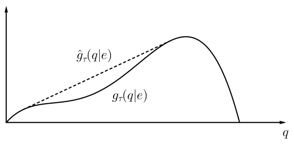
Figure 1: Ironed objective function

Finally, we prove the above claim to complete the proof of Section 3.2.

By the definition of $\hat{g}_{\tau}(q|e)$, for any randomized price $p$,

$$\displaystyle\operatorname*{\mathbb{E}}_{p}[g_{\tau}(D_{\tau}(p|e)|e)]\leq\operatorname*{\mathbb{E}}_{p}[\hat{g}_{\tau}(D_{\tau}(p|e)|e)].$$

Since $\hat{g}$ is concave, applying Jensen’s inequality yields:

$$\displaystyle\operatorname*{\mathbb{E}}_{p}[\hat{g}_{\tau}(D_{\tau}(p|e)|e)]\leq\hat{g}_{\tau}\left(\operatorname*{\mathbb{E}}_{p}[D_{\tau}(p|e)]\big{|}e\right)=\hat{g}_{\tau}(\bar{q}|e)$$

Now it suffices to show that the upper bound $\hat{g}_{\tau}(\bar{q}|e)$ is attainable.

If $\hat{g}_{\tau}(\bar{q}|e)=g_{\tau}(\bar{q}|e)$, then the right-hand-side could be achieved by letting $p_{\tau}(e)$ be the deterministic price $D^{-1}_{\tau}(\bar{q}|e)$.

Otherwise, let $I=(q^{\prime},q^{\prime\prime})$ be the ironed interval (where $\hat{g}_{\tau}(q|e)>g_{\tau}(q|e),\forall q\in I$ but $\hat{g}_{\tau}(q^{\prime}|e)=g_{\tau}(q^{\prime}|e)$ and $\hat{g}_{\tau}(q^{\prime\prime}|e)=g_{\tau}(q^{\prime\prime}|e)$) containing $\bar{q}$. Thus $\bar{q}$ can be written as a convex combination of the end points $q^{\prime}$ and $q^{\prime\prime}$: $\bar{q}=\lambda q^{\prime}+(1-\lambda)q^{\prime\prime}$. Note that the function $\hat{g}_{\tau}$ is linear within the interval $I$. Therefore

$$\displaystyle\lambda g_{\tau}(q^{\prime}|e)+(1-\lambda)g_{\tau}(q^{\prime\prime}|e)=\lambda\hat{g}_{\tau}(q^{\prime}|e)+(1-\lambda)\hat{g}_{\tau}(q^{\prime\prime}|e)=\hat{g}_{\tau}(\lambda q^{\prime}+(1-\lambda)q^{\prime\prime}|e)=\hat{g}_{\tau}(\bar{q}|e).$$

In other words, the upper bound $\hat{g}_{\tau}(\bar{q}|e)$ could be achieved by setting the price to be $q^{\prime}$ with probability $\lambda$ and $q^{\prime\prime}$ with probability $1-\lambda$. In the meanwhile, the flow $q_{\tau}(e)$ would retain the same. ∎

Proof of Theorem 3.1.

The theorem is implied by Section 3.1 and Section 3.2. In particular, the reward function is the ironed objective function $\hat{g}$. ∎

In the rest of the paper, we will focus on the following equivalent problem:

maximize $$\sum_{e,\tau}\hat{g}_{\tau}(q_{\tau}(e)|e)$$ (3.2)

subject to $$\hyperref@@ii[eq:feasible]{(\ref*{eq:feasible})}~{}\text{and}~{}\hyperref@@ii[eq:strans]{(\ref*{eq:strans})}.$$

4 Optimal Solution in Static Environment

In this setting, we restrict our attention to the case where the environment is static, hence the objective function does not change over time, i.e., $\forall\tau\in[T],\hat{g}_{\tau}(q|e)\equiv\hat{g}(q|e)$. We aim to find the optimal stationary policy that maximizes the objective function, i.e., the decisions $q_{\tau}$ depends only on the current state $w_{\tau}$.

In this section, we discretize the MDP problem and focus on stable policies. With the introduction of the ironed objective function $\hat{g}_{\tau}$, we show that for any discretization scheme, the optimal stationary policy of the induced discretized MDP is dominated by a stable dispatching scheme. Then we formulate the stable dispatching scheme as a convex problem, which means the optimal stationary policy can be found in polynomial time.

Definition .

A stable dispatching scheme is a pair of state and policy $(w_{\tau},\pi)$, such that if policy $\pi$ is applied, the distribution of available drivers does not change over time, i.e., $w_{\tau+1}(v)=w_{\tau}(v)$.

In particular, under a stable dispatching scheme, the state transition rule (3.1) is equivalent to the following form:

$$\displaystyle\sum_{e\in\mathrm{OUT}(v)}q(e)=\sum_{e\in\mathrm{IN}(v)}q(e).$$ (4.1)

Definition .

Let $\mathcal{M}=(G,D,\hat{g},S,A,W)$ be the original MDP problem. A discretized MDP $\mathcal{DM}$ with respect to $\mathcal{M}$ is a tuple $(G_{d},D_{d},\hat{g}_{d},S_{d},A_{d},W_{d})$, where $G_{d}=G$, $D_{d}=D$, $\hat{g}_{d}=\hat{g}$, $W_{d}=W$, $S_{d}$ is a finite subset of $S$, and $A_{d}$ is a finite subset of $A$ that contains all feasible transition flows between every two states in $S_{d}$.

Theorem 4.1.

Let $\mathcal{DM}$ and $\mathcal{M}$ be a discretized MDP and the corresponding original MDP. Let $\pi_{d}:S_{d}\to A_{d}$ be an optimal stationary policy of $\mathcal{DM}$. Then there exists a stable dispatching scheme $(w,\pi)$, such that the time-average objective of $\pi$ in $\mathcal{M}$ is no less than that of $\pi_{d}$ in $\mathcal{DM}$.

Proof.

Consider policy $\pi_{d}$ in $\mathcal{DM}$. Starting from any state in $S_{d}$ with policy $\pi_{d}$, let $\{w_{\tau}\}_{0}^{\infty}$ be the subsequent state sequence. Since $\mathcal{DM}$ has finitely many states and policy $\pi_{d}$ is a stationary policy, there must be an integer $n$, such that $w_{n}=w_{m}$ for some $m<n$ and from time step $m$ on, the state sequence become a periodic sequence. Define

$$\displaystyle\bar{w}=\frac{1}{n-m}\sum_{k=m}^{n-1}w_{k},\quad\bar{q}=\frac{1}{n-m}\sum_{k=m}^{n-1}\pi_{d}(w_{k})$$

Denote by $\pi_{d}(w_{k}|e)$ or $q_{d}(e)$ the flow at edge $e$ of the decision $\pi_{d}(w_{k})$. Sum the transition equations for all the time steps $m\leq k<n$, and we get:

$$\displaystyle\sum_{k=m}^{n-1}w_{k+1}(v)-\sum_{k=m}^{n-1}w_{k}(v)=\displaystyle\sum_{k=m}^{n-1}\left(\sum_{\mathrm{IN}(v)}\pi_{d}(w_{k}|e)\right)-\sum_{k=m}^{n-1}\left(\sum_{\mathrm{OUT}(v)}\pi_{d}(w_{k}|e)\right)$$

$$\displaystyle\bar{w}(v)=\bar{w}(v)-\left(\sum_{\mathrm{OUT}(v)}\bar{q}(e)\right)+\left(\sum_{\mathrm{IN}(v)}\bar{q}(e)\right)$$

Also, policy $\pi_{d}$ is a valid policy, so $\forall v\in V$ and $\forall m\leq k<n$:

$$\displaystyle\sum_{\mathrm{OUT}(v)}q_{k}(e)\leq w_{k}(v)$$

Summing over $k$, we have:

$$\displaystyle\sum_{\mathrm{OUT}(v)}\bar{q}(e)\leq\bar{w}(v)$$

Now consider the original problem $\mathcal{M}$. Let $w=\bar{w}$ and $\pi$ be any stationary policy such that:

• $\pi(w)=\bar{q}$;

• starting from any state $w^{\prime}\neq w$, policy $\pi$ leads to state $w$ within finitely many steps.

Note that the second condition can be easily satisfied since the graph $G$ is strongly connected.

With the above definitions, we know that $(w,\pi)$ is a stable dispatching scheme. Now we compare the objectives of the two policies $\pi_{d}$ and $\pi$. The time-average objective function is not sensitive about the first finitely many immediate objectives. And since the state sequences of both policies $\pi_{d}$ and $\pi$ are periodic, Their time-average objectives can be written as:

$$\displaystyle\mathrm{OBJ}(\pi_{d})=\frac{1}{n-m}\sum_{k=m}^{n-1}\sum_{e\in E}\hat{g}(q_{d}(e)|e)$$

$$\displaystyle\mathrm{OBJ}(\pi)=\sum_{e\in E}\hat{g}(\bar{q}(e)|e)$$

By Jensen’s inequality, we have:

$$\mathrm{OBJ}(\pi_{d})\displaystyle=\frac{1}{n-m}\sum_{k=m}^{n-1}\sum_{e\in E}\hat{g}(q_{d}(e)|e)\displaystyle\leq\sum_{e\in E}\hat{g}\left[\left(\frac{1}{n-m}\sum_{k=m}^{n}q_{d}(e)\right)\big{|}e\right]\displaystyle=\sum_{e\in E}\hat{g}(\bar{q}(e)|e)=\mathrm{OBJ}(\pi)$$

∎

With Theorem 4.1, we know there exists a stable dispatching scheme that dominates the optimal stationary policy of the our discretized MDP. Thus we now only focus on stable dispatching schemes. The problem of finding an optimal stable dispatching scheme can be formulated as a convex program with linear constraints:

maximize $$\sum_{e\in E}\hat{g}(q|e)$$ (4.2)

subject to $$\hyperref@@ii[eq:feasible]{(\ref*{eq:feasible})}~{}\text{and}~{}\hyperref@@ii[eq:ststrans]{(\ref*{eq:ststrans})}.$$

Because $\hat{g}(q|e)$ is concave, the program is convex. Since all convex programs can be solved in polynomial time, our algorithm for finding optimal stationary policy of maximizing the objective functions is efficient.

5 Characterization of optimality

In this section, we characterize the optimal solution via dual analysis. For the ease of presentation, we consider Program 4.2 in the static environment with infinite horizon. Our characterization directly extends to the dynamic environment.

The Lagrangian is defined to be

$$L(q,\lambda,\mu)= \displaystyle-\sum_{e\in E}\hat{g}(q|e)+\lambda\left(\sum_{e\in E}q(e)-1\right)\displaystyle+\sum_{v\in V}\mu_{v}\left(\sum_{\mathrm{OUT}(v)}q(e)-\sum_{\mathrm{IN}(v)}q(e)\right)$$

$$= \displaystyle-\lambda+\sum_{e\in E}\left[-\hat{g}(q|e)+(\lambda+\mu_{s}-\mu_{t})q(e)\right],$$

where $s$ and $t$ are the origin and destination of $e$, i.e., $e=(s,t)$, and $\lambda$ and $\mu$ are Lagrangian multipliers with $\lambda\geq 0$. Note that we implicitly transform program 4.2 to the standard form that minimizes the objective $-\sum_{e\in E}\hat{g}(q^{*}|e)$.

The Lagrangian dual function is

$$\displaystyle h(\lambda,\mu)=\inf_{q}L(q,\lambda,\mu)=\sum_{e\in E}\left[-\hat{g}(\tilde{q}|e)+(\lambda+\mu_{s}-\mu_{t})\tilde{q}(e)\right],$$

where $\tilde{q}(e)$ is a function of $\lambda$ and $\mu$ such that $\lambda+\mu_{s}-\mu_{t}=\hat{g}^{\prime}(\tilde{q}|e)$, where $\hat{g}^{\prime}(\tilde{q}|e)$ is the derivative of the objective function with respect to flow $q$. The dual program corresponding to Program 4.2 is

maximize $$h(\lambda,\mu)$$ (5.1)

subject to $$\lambda\geq 0$$

According to the KKT conditions, we have the following characterization for optimal solutions.

Theorem 5.1.

Let $q^{*}(e)$ be a feasible solution to the primal program 4.2 and $(\lambda^{*},\mu^{*})$ be a feasible solution to the dual program 5.1. Then both $q^{*}(e)$ and $(\lambda^{*},\mu^{*})$ are primal and dual optimal with $-\sum_{e\in E}\hat{g}(q^{*}|e)=h(\lambda^{*},\mu^{*})$, if and only if

$$\displaystyle\lambda^{*}\left(\sum_{e\in E}q^{*}(e)-1\right)=0$$ (5.2)

$$\hat{g}^{\prime}(q^{*}|e)=\lambda^{*}+\mu_{s}^{*}-\mu_{t}^{*},\forall v\in V$$ (5.3)

Proof.

According to the definition of $h(\lambda,\mu)$, we have $h(\lambda^{*},\mu^{*})=\inf_{q}L(q,\lambda^{*},\mu^{*})$. Since $\hat{g}(q|e)$ are concave functions, Equation 5.3 is equivalent to the fact that $q^{*}(e)$ minimizes the function $L(q,\lambda^{*},\mu^{*})$.

$$h(\lambda^{*},\mu^{*})= \displaystyle\inf_{q}L(q,\lambda^{*},\mu^{*})$$

$$= L(q^{*},\lambda^{*},\mu^{*})$$

$$= \displaystyle-\sum_{e\in E}\hat{g}(q^{*}|e)+\lambda^{*}\left(\sum_{e\in E}q^{*}(e)-1\right)\displaystyle+\sum_{v\in V}\mu^{*}_{v}\left(\sum_{\mathrm{OUT}(v)}q^{*}(e)-\sum_{\mathrm{IN}(v)}q^{*}(e)\right)$$

$$= \displaystyle-\sum_{e\in E}\hat{g}(q^{*}|e),$$

where the last equation uses the Equation 5.2 and the fact that $q^{*}(e)$ is feasible. ∎

Continuing with Theorem 5.1, we will analyze the dual variables from the economics angle and some interesting insights into this problem for real applications.

5.1 Economic interpretation

The dual variables have useful economic interpretations (see (Boyd and Vandenberghe, 2004, Chapter 5.6)). $\lambda^{*}$ is the system-wise marginal contribution of the drivers (i.e. the increase in the objective function when a small amount of drivers are added to the system). Note that by the complementary slackness (Equation 5.2), if $\lambda^{*}>0$, the sum of the total flow must be $1$, meaning that all drivers are busy, and more requests can be accepted (hence increase revenue) if more drivers are added to the system. Otherwise, there must be some idle drivers, and adding more drivers cannot increase the revenue.

$\mu_{v}^{*}$ is the marginal contribution of the drivers at node $v$. If we allow the outgoing flow from node $v$ to be slightly more than the incoming flow to node $v$, then $\mu_{v}$ is the revenue gain from adding more drivers at node $v$.

5.2 Insights for applications

The way we formulate and solve the problem, in fact, naturally leads to two interesting insights into this problem, which are potentially useful for real applications.

1. Scalability

In our model, the size of the convex program increases linearly in the number of edges, hence quadratically in the number of regions. This could be one hidden feature that is potentially an obstacle to real applications, where the number of regions in a city might be quite large.

A key observation to the issue is that any dispatching policy induced by a real system is a feasible solution of our convex program and any improvement (maybe via gradient descent) from such policy in fact leads to a better solution for this system. In other words, it might be hard to find the exact optimal or nearly optimal solutions, but it is easy to improve from the current state. Therefore, in practice, the platform can keep running the optimization in background and apply the most recent policy to gain more revenue (or achieve a higher value of some other objectives).

2. Alternative solution

As suggested by the characterization and its economic interpretation, instead of solving the convex programs directly, we also have an alternative way to find the optimal policy by solving the dual program. The optimal policy can be easily recovered from dual optimal solutions. In particular, according to the economic interpretation of dual variables, we need to estimate the marginal contributions of drivers.

More importantly, the number of dual variables ($=$ the number of regions) is much smaller than the number of primal variables ($=$ the number of edges $\approx$ square of the former). So solving the dual program may be more efficient when applied to real systems, and is also of independent interest of this paper.

6 Empirical Analysis

We design experiments to demonstrate the good performance of our algorithms for real applications. In this section, we first describe the dataset and then introduce how to extract useful information for our model from the dataset. Two benchmark policies, FIXED and SURGE, are compared with our pricing policy. The result analysis includes demand-supply balance and instantaneous revenue in both static and dynamic environments.

6.1 Dataset

We perform our empirical analysis based on a public dataset from a major ride-sharing company. The dataset includes the orders in a city for three consecutive weeks and the total number of orders is more than $8.5$ million. An order is created when a passenger send a ride request to the platform.

Each order consists of a unique order ID, a passenger ID, a driver ID, an origin, a destination, and an estimated price, and the timestamp when the order is created (see Table 1 for example). The driver ID might be empty if no driver was assigned to pick up the passenger. There are $66$ major regions of the city and the origins and destinations in the dataset are given as the region IDs. We say a request is related to a region if the region is either the origin or the destination of the request. And the popularity of a region is defined as the number of related requests. Since some of the regions in the dataset have very low popularity values, we only consider the most popular $21$ or $5$ regions in the two settings (see Section 6.4 and Section 6.5 respectively for details). The related requests of the most popular $21$ (or $5$) regions cover about $90\%$ (or $50\%$) of the total requests in the original dataset.

For ease of presentation, we relabel the region IDs in descending order of their popularities (so region #$1$ is the most popular region). Figure 2 illustrates the frequencies of requests on different origin-destination pairs. From the figure, one can see that the frequency matrix is almost symmetric and the destination of a request is most likely to be in the same region as the origin.

order	driver	user	origin	dest	price	timestamp
hash	hash	hash	hash	hash	$37.5$	01-15 00:35:11

Table 1: An example of a row in the dataset, where “hash” stands for some hash strings of the IDs that we didn’t show the exact value here.

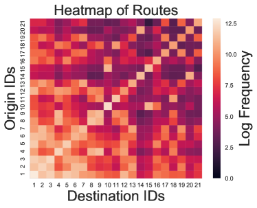
1

Figure 2: The logarithmic frequencies of request routes.

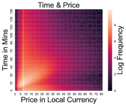
(a) Time & price without filtering

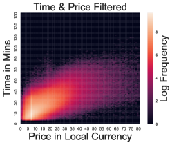
(b) Time & price with filtering

1

Figure 3: The logarithmic frequencies of $(\text{time},~{}\text{price})$ pairs, with or without filtering the “abnormal” requests.

6.2 Data preparation

The time consumptions from nodes to nodes and demand curves for edges are known in our model. However, the dataset doesn’t provide such information directly. We filter out "abnormal" requests and apply a linear regression to get the relationship of the travel time and the price. It makes possible to infer the travel time from the order price. For the demand curves, we observe the values of each edge and fit them to lognormal distributions.

Distance and travel time

The distance (or equivalently the travel time) from one region to another is required to perform our simulation. We approximate the travel time by the time interval of two consecutive requests assigned to the same driver. In Figure 3(a), we plot the frequencies of requests with certain (time, price) pairs. We cannot see clear relationship between time and price, which are supposed to be roughly linearly related in this figure. We think that this is due to the existence of two types of “abnormal” requests:

• Cancelled requests, usually with very short completion time but not necessarily low prices (appeared in the right-bottom part of the plot);

• The last request of a working period, after which the driver might go home or have a rest. These requests usually have very long completion time but not necessarily high enough prices (appeared in the left-top part of the plot).

With the observations above, we filter out the requests with significantly longer or shorter travel time compared with most of the requests with the same origin and destination. Figure 3(b) illustrates the frequencies of requests after such filtering. As expected, the brightest region roughly surrounds the $30^{\circ}$ line in the figure. By applying a standard linear regression, the slope turns out to be approximately $0.5117$ CNY per minute. One may also notice some “right-shifting shadows” of the brightest region, which are caused by the surge-pricing policy with different multipliers.

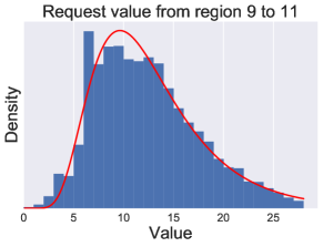
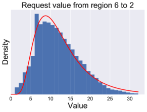
1

Figure 4: Fitting request values to lognormal distributions.

Estimation of demand curves

To estimate the demand curves, we first gather all the requests along the same edge (also within the same time period for dynamic environment, see Section 6.5) and take the prices associated with the requests as the values of the passengers. Then, we fit the values of each edge (and each time period for dynamic environment) to a lognormal distribution. The reason that we choose the lognormal distribution is two-fold: (i) the data fits lognormal distributions quite well (see Figure 4 as examples); (ii) lognormal distributions are commonly used in some related literatures Ostrovsky and Schwarz (2011); Lahaie and Pennock (2007); Roberts et al. (2016); Shen and Tang (2017).

We set the cost of traveling to be zero, because we do not have enough information from the dataset to infer the cost.

6.3 Benchmarks

We consider two benchmark policies:

• FIXED: fixed per-minute pricing, i.e., the price of a ride equals to the estimated traveling time from the origin to the destination of this ride multiplied by a per-minute price $\alpha$, where $\alpha$ is a constant across the platform.

• SURGE: based on FIXED policy, using surge pricing to clear the local market when supply is not enough. In other words, the price of a ride equals to the estimated traveling time multiplied by $\alpha\beta$, where $\alpha$ is the fixed per-minute price and $\beta\geq 1$ is the surge multiplier. Note that $\beta$ is dynamic and can be different for requests initiated at different regions, while the requests initiated at the same regions will share the same surge multipliers.

In the rest of this section, we evaluate and compare our dynamic pricing policy DYNAM with these two benchmarks in both static and dynamic environments.

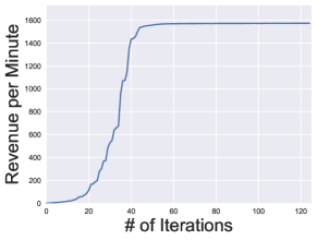
(a) Static environment

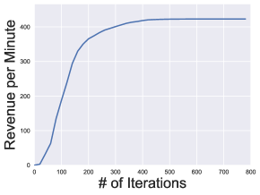
(b) Dynamic environment

1

Figure 5: Convergence of revenue.

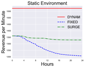
(a) Static environment

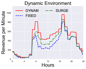
(b) Dynamic environment

1

Figure 6: Instantaneous revenue in different environments.

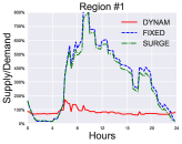
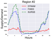
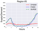
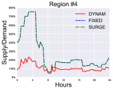
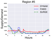
Figure 7: Instantaneous supply ratios for different regions.

6.4 Static environment

We first present the empirical analysis for the static environment, which is simpler than the dynamic environment that we will consider next, hence easier to begin with.

In the static environment, we use the average of the statistics of all $21$ days as the inputs to our model. For example, the demand function $D(p|e)$ is estimated based on the frequencies and prices of the requests along edge $e$ averaged over time. Similarly, the total supply of drivers is estimated based on the total durations of completed requests.

With the static environment, we can instantiate the convex program (4.2) and solve via standard gradient descent algorithms. In our case, we simply use the MATLAB function fmincon to solve the convex program on a PC with Intel i5-3470 CPU. We did not apply any additional techniques to speed-up the computation as the optimization of running time is not the main focus of this paper. Figure 5(a) illustrates the convergence of the objective value (revenue) with increasing number of iterations, where each iteration roughly takes $0.2$ second.

To compare the performance of policy DYNAM with the benchmark policies FIXED and SURGE, we also simulates them under the same static environment. In particular, the length of each timestep is set to be $15$ minutes and the number of steps in simulation is $96$ (so $24$ hours in total). For both FIXED and SURGE, we use the per-minute price fitted from data as the base price, $\alpha=0.5117$, and allow the surge ratio $\beta$ to be in $[1.0,5.0]$. To make the evaluations comparable, we use the distribution of drivers under the stationary solution of our convex program as the initial driver distributions for FIXED and SURGE. Figure 6(a) shows how the instantaneous revenues evolve as the time goes by, where DYNAM on average outperforms FIXED and SURGE by roughly $24\%$ and $17\%$, respectively.

Note that our policy DYNAM is stationary under the static environment, the instantaneous revenue is constant (the red horizontal line). Interestingly, the instantaneous revenue curves of both FIXED and SURGE are decreasing and the one of FIXED is decreasing much faster. The observation reflects that both FIXED and SURGE are not doing well in dispatching the vehicles: FIXED simply never balances the supply and demand, while SURGE shows better control in the balance of supply and demand because the policy seeks to balance the demand with local supply when supply can not meet the demand. However, neither of them really balance the global supply and demand, so the instantaneous revenue decrease as the supply and demand become more unbalanced.

In other words, the empirical analysis supports our insight about the importance of vehicle dispatching in ride-sharing platforms.

6.5 Dynamic environment

In the dynamic environment, the parameters (i.e., the demand functions and the total number of requests) are estimated based on the statistics of each hour but averaged over different days. For example, the demand functions $D_{h}(p|e)$ are defined for each edge $e$ and each of the $24$ hours, $h\in\{0,\ldots,23\}$. In particular, we only use the data from the weekdays ($14$ days in total) among the most popular $5$ regions for the estimation.

Again, we instantiate the convex program (3.2) for the dynamic environment and solve via the fmincon function on the same PC that we used for the static case. Figure 5(b) shows the convergence of the objective value with increasing number of iterations, where each iteration takes less than $1$ minute.

We setup FIXED and SURGE in exactly the same way as we did for the static environment, except that the initial driver distribution is from the solution of the convex program for dynamic environment.

Figure 6(b) shows the instantaneous revenue along the simulation. In particular, the relationship $\texttt{DYNAM}\succ\texttt{SURGE}\succ\texttt{FIXED}$ holds almost surely. Moreover, the advantages of DYNAM over the other two policies are more significant at the high-demand “peak times”. For example, at $8$ a.m., DYNAM ($\sim$$800$) outperforms SURGE ($\sim$$600$) and FIXED ($\sim$$500$) by roughly $33\%$ and $60\%$, respectively.

Demand-supply balance

Balancing the demand and supply is not the goal of our dispatching policy. However, a policy without such balancing abilities are unlikely to perform well. In Figure 7, we plot the supply ratios (defined as the local instantaneous supply divided by the local instantaneous demand) for all the $5$ regions during the $24$ hours of the simulation.

From the figures, we can easily check that comparing with the other two lines, the red line (the supply ratio of DYNAM) tightly surrounds the “balance” line of $100\%$, which means that the number of available drivers at any time and at each region is close to the number of requests sent from that region at that time. The lines of other two policies sometimes could be very far from the “balance” line, that is, the drivers under policy FIXED and SURGE are not in the location where many passengers need the service.

As a result, our policy DYNAM shows much stronger power in vehicle dispatching and balancing demand and supply in dynamic ride-sharing systems. Such advanced techniques in dispatching can in turn help the platform to gain higher revenue through serving more passengers.

References

- (1)
- Alonso-Mora et al. (2017) Javier Alonso-Mora, Samitha Samaranayake, Alex Wallar, Emilio Frazzoli, and Daniela Rus. 2017. On-demand high-capacity ride-sharing via dynamic trip-vehicle assignment. PNAS (2017), 201611675.
- Balseiro et al. (2017) Santiago Balseiro, Max Lin, Vahab Mirrokni, Renato Paes Leme, and Song Zuo. 2017. Dynamic revenue sharing. In NIPS 2017.
- Banerjee et al. (2017) Siddhartha Banerjee, Daniel Freund, and Thodoris Lykouris. 2017. Pricing and Optimization in Shared Vehicle Systems: An Approximation Framework. In EC 2017.
- Banerjee et al. (2015) Siddhartha Banerjee, Carlos Riquelme, and Ramesh Johari. 2015. Pricing in Ride-share Platforms: A Queueing-Theoretic Approach. (2015).
- Bimpikis et al. (2016) Kostas Bimpikis, Ozan Candogan, and Saban Daniela. 2016. Spatial Pricing in Ride-Sharing Networks. (2016).
- Boyd and Vandenberghe (2004) Stephen Boyd and Lieven Vandenberghe. 2004. Convex optimization. Cambridge university press.
- Cachon et al. (2016) Gerard P Cachon, Kaitlin M Daniels, and Ruben Lobel. 2016. The role of surge pricing on a service platform with self-scheduling capacity. (2016).
- Castillo et al. (2017) Juan Camilo Castillo, Dan Knoepfle, and Glen Weyl. 2017. Surge pricing solves the wild goose chase. In EC 2017. ACM, 241–242.
- Chan and Shaheen (2012) Nelson D Chan and Susan A Shaheen. 2012. Ridesharing in north america: Past, present, and future. Transport Reviews 32, 1 (2012), 93–112.
- Chen and Sheldon (2015) M Keith Chen and Michael Sheldon. 2015. Dynamic pricing in a labor market: Surge pricing and flexible work on the Uber platform. Technical Report. Mimeo, UCLA.
- Cramer and Krueger (2016) Judd Cramer and Alan B Krueger. 2016. Disruptive change in the taxi business: The case of Uber. The American Economic Review 106, 5 (2016), 177–182.
- Crawford and Meng (2011) Vincent P Crawford and Juanjuan Meng. 2011. New york city cab drivers’ labor supply revisited: Reference-dependent preferences with rationalexpectations targets for hours and income. AER 101, 5 (2011), 1912–1932.
- Fang et al. (2017) Zhixuan Fang, Longbo Huang, and Adam Wierman. 2017. Prices and subsidies in the sharing economy. In Proceedings of the 26th International Conference on World Wide Web. WWW 2017, 53–62.
- Gale and Holmes (1993) Ian L Gale and Thomas J Holmes. 1993. Advance-purchase discounts and monopoly allocation of capacity. The American Economic Review (1993), 135–146.
- Gendreau et al. (1994) Michel Gendreau, Alain Hertz, and Gilbert Laporte. 1994. A tabu search heuristic for the vehicle routing problem. Management science 40, 10 (1994), 1276–1290.
- Ghiani et al. (2003) Gianpaolo Ghiani, Francesca Guerriero, Gilbert Laporte, and Roberto Musmanno. 2003. Real-time vehicle routing: Solution concepts, algorithms and parallel computing strategies. European Journal of Operational Research 151, 1 (2003).
- Iglesias et al. (2016) Ramon Iglesias, Federico Rossi, Rick Zhang, and Marco Pavone. 2016. A BCMP Network Approach to Modeling and Controlling Autonomous Mobility-on-Demand Systems. arXiv preprint arXiv:1607.04357 (2016).
- Kostiuk (1990) Peter F Kostiuk. 1990. Compensating differentials for shift work. Journal of political Economy 98, 5, Part 1 (1990), 1054–1075.
- Lahaie and Pennock (2007) Sébastien Lahaie and David M Pennock. 2007. Revenue analysis of a family of ranking rules for keyword auctions. In EC 2007. ACM, 50–56.
- Laporte (1992) Gilbert Laporte. 1992. The vehicle routing problem: An overview of exact and approximate algorithms. European journal of operational research 59, 3 (1992).
- Ma et al. (2013) Shuo Ma, Yu Zheng, and Ouri Wolfson. 2013. T-share: A large-scale dynamic taxi ridesharing service. In ICDE. IEEE, 410–421.
- McAfee and Te Velde (2006) R Preston McAfee and Vera Te Velde. 2006. Dynamic pricing in the airline industry. forthcoming in Handbook on Economics and Information Systems, Ed: TJ Hendershott, Elsevier (2006).
- Moreira-Matias et al. (2013) Luis Moreira-Matias, Joao Gama, Michel Ferreira, Joao Mendes-Moreira, and Luis Damas. 2013. Predicting taxi–passenger demand using streaming data. IEEE Transactions on Intelligent Transportation Systems 14, 3 (2013), 1393–1402.
- Oettinger (1999) Gerald S Oettinger. 1999. An empirical analysis of the daily labor supply of stadium venors. Journal of political Economy 107, 2 (1999), 360–392.
- Ostrovsky and Schwarz (2011) Michael Ostrovsky and Michael Schwarz. 2011. Reserve prices in internet advertising auctions: A field experiment. In EC 2011Practical. ACM, 59–60.
- Roberts et al. (2016) Ben Roberts, Dinan Gunawardena, Ian A Kash, and Peter Key. 2016. Ranking and tradeoffs in sponsored search auctions. ACM Transactions on Economics and Computation 4, 3 (2016), 17.
- Shen and Tang (2017) Weiran Shen and Pingzhong Tang. 2017. Practical versus Optimal Mechanisms. In AAMAS. 78–86.
- Stavins (2001) Joanna Stavins. 2001. Price discrimination in the airline market: The effect of market concentration. Review of Economics and Statistics 83, 1 (2001), 200–202.
- Tang et al. (2016) Christopher S Tang, Jiaru Bai, Kut C So, Xiqun Michael Chen, and Hai Wang. 2016. Coordinating supply and demand on an on-demand platform: Price, wage, and payout ratio. (2016).
- Tong et al. (2017) Yongxin Tong, Yuqiang Chen, Zimu Zhou, Lei Chen, Jie Wang, Qiang Yang, Jieping Ye, and Weifeng Lv. 2017. The simpler the better: a unified approach to predicting original taxi demands based on large-scale online platforms. In KDD 2017. ACM, 1653–1662.
- Zhao et al. (2014) Dengji Zhao, Dongmo Zhang, Enrico H Gerding, Yuko Sakurai, and Makoto Yokoo. 2014. Incentives in ridesharing with deficit control. In AAMAS 2014.