Invex Optimization Revisited

Abstract

Given a non-convex optimization problem, we study conditions under which every Karush-Kuhn-Tucker (KKT) point is a global optimizer. This property is known as KT-invexity and allows to identify the subset of problems where an interior point method always converges to a global optimizer. In this work, we provide necessary conditions for KT-invexity in n-dimensions and show that these conditions become sufficient in the two-dimensional case. As an application of our results, we study the Optimal Power Flow problem, showing that under mild assumptions on the variable’s bounds, our new necessary and sufficient conditions are met for problems with two degrees of freedom.

Notations

$\partial S$	boundary of a set $S$.
$x_{i}$	$i$th component of vector $\vec{x}$.
$f^{\prime}_{x_{i}}=\frac{\partial f}{\partial x_{i}}$	partial derivative of $f$ with respect to $x_{i}$.
$||\vec{x}||$	Euclidean norm of vector $\vec{x}$.
$\vec{x}\cdot\vec{y}$	the dot product of vectors $\vec{x}$ and $\vec{y}$.
$\vec{x}^{T}$	the transpose of vector $\vec{x}$.
$\overline{AB}$	a segment between two points.
$2\mathbb{N},~{}2\mathbb{N}{+}1$	the sets of even and odd numbers.
$f^{\prime}_{-}(x),f^{\prime}_{+}(x)$	left and right derivatives of $f$.
$sign(x)$	the sign function.

1 Introduction

Convexity plays a central role in mathematical optimization. Under constraint qualification conditions wang2013constraint , the Karush-Kuhn-Tucker (KKT) necessary optimality conditions become also sufficient for convex programs boyd2004convex . In addition, convexity of the constraints is used to prove convergence (and rates of convergence) of specialized algorithms nesterov1994interior . However, real-world problems often describe non-convex regions, and relaxing the convexity assumption while maintaining some optimality properties is highly desirable.

One such property, called Kuhn-Tucker invexity, is the sufficiency of KKT conditions for global optimality:

Definition 1

martin1985essence An optimization problem is said to be Kuhn-Tucker invex (KT-invex) if every KKT point is a global optimizer.

Various notions of generalized convexity have been proposed in the literature. Early generalizations include pseudo- and quasi-convexity introduced by Mangasarian in mangasarian1965pseudo where he also proves that problems with a pseudo-convex objective and quasi-convex constraints are KT-invex. Hanson hanson1981sufficiency defined the concept of invex functions and gave a sufficient condition for KT-invexity, which was relaxed by Martin martin1985essence in order to obtain a condition that is both necessary and sufficient. Later on, Craven craven1985invex investigated the properties of invex functions.

These ideas inspired more research on generalized convexity. K-invex craven1981invex , preinvex ben1986invexity , B-vex bector1991b , V-invex jeyakumar1992generalised , (p,r)-invex antczak2001p and other types of functions and their roles in mathematical optimization.

However, to the best of our knowledge, there are no computationally efficient procedures to check KT-invexity in practice even when restricted to two-dimensional spaces. To address this problem, we propose a new set of conditions expressed in terms of the behavior of the objective function on the boundary of the feasible set. We prove that these conditions are necessary and, for two-dimensional problems, sufficient for KT-invexity.

The paper is organized as follows. In Section 2 we introduce the notion of boundary-invexity and study its connection to the local optimality of KKT points. Here we also establish the connection between global optimality on the boundary and in the interior. Section 3 gives the definition of a two-dimensional cross product. In Section 4 we define a parametrization of the boundary curve. In Section 5 we study the behavior of concave functions on a line and present some results on boundary-optimality. Section 6 presents the main theorem establishing the sufficiency of boundary-invexity for two-dimensional problems. Finally, Section 7 investigates boundary-invexity of the Optimal Power Flow problem and Section 8 concludes the paper.

2 Conditions for Kuhn-Tucker invexity

Consider the optimization problem:

max $$f(\vec{x})$$

s.t. $$g_{i}(\vec{x})\leq 0~{}\forall i=1..m$$ (NLP)

$$\vec{x}\in\mathbb{R}^{n},$$

where all functions $f(\vec{x})$, $g(\vec{x})$ and $h(\vec{x})$ are twice continuously differentiable and $f(\vec{x})$ is concave. The results in this paper can be extended to problems with quasiconcave objective functions since only convexity of the superlevel sets of $f$ is used in the proofs.

Let $F$ denote the feasible set of (2).

Definition 2

wright1999numerical A solution $\vec{x}^{*}$ of problem (2) is said to satisfy Karush-Kuhn-Tucker (KKT) conditions if there exist constants $\mu_{i}~{}(i=1,...,m)$, called KKT multipliers, such that

$$\nabla f(\vec{x}^{*})=\sum_{i=1}^{m}\mu_{i}\nabla g_{i}(\vec{x}^{*}),$$ (1)

$$g_{i}(\vec{x}^{*})\leq 0,~{}\forall i=1,...,m,$$ (2)

$$\mu_{i}\geq 0,~{}\forall i=1,...,m,$$ (3)

$$\mu_{i}g_{i}(\vec{x})=0,~{}\forall i=1,...,m.$$ (4)

Points that satisfy KKT conditions are referred to as KKT points.

Definition 3

wright1999numerical A point $\vec{x}^{*}\in\mathbb{R}^{n}$ is a local maximizer for (2) if $\vec{x}^{*}\in F$ and there is a neighborhood $N(\vec{x}^{*})$ such that $f(\vec{x})\leq f(\vec{x}^{*})$ for $\vec{x}\in N(\vec{x}^{*})\cap F$.

Let us emphasize that checking local optimality is NP-hard in general:

Theorem 2.1

pardalos1988checking The problem of checking local optimality for a feasible solution of (2) is NP-hard.

In this work, we try to investigate necessary and sufficient conditions that allow us to circumvent the negative result presented in Theorem 2.1 by identifying problems where KKT points are provably global optimizers.

2.1 Weak boundary-invexity

For each non-convex constraint $g_{i}(x)\leq 0$ define the problem:

$$\min~{}f(\vec{x})$$ (NLP_i)

$$s.t.~{}g_{i}(\vec{x})=0.$$

Definition 4

(Weak boundary-invexity) Problem (2) is weakly boundary-invex if (NLP_i) is unbounded or at least one of the following holds for its global minimum $\vec{x}^{*}$:

1. $\vec{x}^{*}$ is infeasible for (2),

2. $\vec{x}^{*}$ is not a strict minimizer,

3. the KKT multiplier for $\vec{x}^{*}$ in (NLP_i) is non-negative,

4. there exist constraints $g_{j}(\vec{x})\leq 0,~{}j\neq i$ in (2) that are active at $\vec{x}^{*}$.

(NLP_i) is still a non-convex problem, and finding its global optimum can be NP-hard in general. However, in some special cases (NLP_i) can be more tractable than (2) since we are restricting the feasible region to one of its boundaries.

For instance, when both $f(\vec{x})$ and $g_{i}(\vec{x})$ are quadratic functions we can apply an extension of the S-lemma:

Theorem 2.2

Xia2016 Let $f(\vec{x})=\vec{x}^{T}A\vec{x}+a^{T}\cdot\vec{x}+c$ and $g(\vec{x})=\vec{x}^{T}B\vec{x}+b^{T}\cdot\vec{x}+d$ be two quadratic functions having symmetric matrices $A$ and $B$. If $g(\vec{x})$ takes both positive and negative values and $B\neq 0$, then the following two statements are equivalent:

1. $(\forall\vec{x}\in\mathbb{R}^{n})~{}g(\vec{x})=0\implies f(\vec{x})\geq 0$,

2. There exists a $\mu\in\mathbb{R}$ such that $f(\vec{x})+\mu g(\vec{x})\geq 0,~{}\forall\vec{x}\in\mathbb{R}^{n}$.

Using this theorem and based on the approach described in Xia2016 , (NLP_i) can be reformulated as a Semidefinite Program and thus solved efficiently.

2.2 Necessary condition for KT-invexity

Theorem 2.3

(Necessary condition) If (2) is KT-invex, then it is weakly boundary-invex.

Proof

We will proceed by contradiction, assume that (2) is KT-invex but not weakly boundary-invex. Thus, there exists a point $\vec{x}^{*}\in F$ which is a global minimizer and therefore a KKT point of (NLP_i):

$$\nabla f(\vec{x}^{*})=-\lambda_{i}\nabla g_{i}(\vec{x}^{*}),$$

$$g_{i}(\vec{x}^{*})=0,$$

$$\lambda_{i}<0.$$

Let $\mu_{i}=-\lambda_{i}$. Since $g_{i}$ is the only active constraint at $\vec{x}^{*}$, we can set $\mu_{j}=0,~{}j=1,...,i-1,i+1,...,m$ and obtain the following system:

$$\nabla f(\vec{x}^{*})=\sum_{j=1}^{m}\mu_{j}\nabla g_{j}(\vec{x}^{*}),$$

$$g_{j}(\vec{x}^{*})=0,~{}\forall j=1,...,m,$$

$$\mu_{j}\geq 0,~{}\forall j=1,...,m,$$

implying that $\vec{x}^{*}$ is a KKT point of (2). Since no other constraints are active at $\vec{x}^{*}$, there exists a point $\hat{\vec{x}}$ in the neighborhood of $\vec{x}^{*}$, such that

$$g_{i}(\hat{\vec{x}})=0\text{ and }\hat{\vec{x}}\in F$$

Since $\vec{x}^{*}$ is a strict global minimizer in (NLP_i), we have that $f(\vec{x}^{*})<f(\hat{\vec{x}})$ which contradicts with (2) being KT-invex.

∎

2.3 Connection between boundary and interior optimality

Definition 5

simmons1963introduction A connected set is a set which cannot be represented as the union of two disjoint non-empty closed sets.

Lemma 1

Given a local maximizer $\vec{x}^{*}\in\mathbb{R}^{n}$ for (2), if $F$ is connected then the following statement is true:
If $\vec{x}^{*}$ is a global maximizer on $\partial F$ then it is also a global maximizer for (2).

Proof

$\vec{x}^{*}$ is a local maximizer, so there is a neighborhood $N(\vec{x}^{*})$ such that if $f(\vec{x})>f(\vec{x}^{*})$ and $\vec{x}\in N(\vec{x}^{*})$, then $\vec{x}\notin F$.

Let us prove the lemma by contradiction. Consider an arbitrary point $\hat{\vec{x}}\in F$ such that $f(\hat{\vec{x}})>f(\vec{x}^{*})$. Since $f$ is concave, there exists a convex set $L_{c}(f)=\{\vec{x}~{}|~{}f(\vec{x})\geq c\}$, where $c$ satisfies $f(\vec{x}^{*})<c<f(\hat{\vec{x}})$. Since $f$ is continuous, $c$ can be chosen so that $\partial L_{c}(f)\cap N(\vec{x}^{*})$ is non-empty. Note that $\hat{\vec{x}}\in L_{c}(f)$.

Since $f(\vec{x})\leq f(\vec{x}^{*})~{}\forall\vec{x}\in\partial F$ and $f(\vec{x})>f(\vec{x}^{*})~{}\forall\vec{x}\in\partial L_{c}(f)$, the two boundaries cannot have common points: $\partial L_{c}(f)\cap\partial F=\emptyset$. Given that $F$ is connected, there are three possibilities:

1) If $F\cap L_{c}(f)=\emptyset$. Contradiction, since $\hat{\vec{x}}\in L_{c}(f)$ would imply that $\hat{\vec{x}}\notin F$.

2) If $F\subset L_{c}(f)$. Contradiction, since $\vec{x}^{*}\in F$ and $\vec{x}^{*}\notin L_{c}(f)$ given that $f(\vec{x}^{*})<c$.

3) If $L_{c}(f)\subset F$. Given that $\partial L_{c}(f)\cap N(\vec{x}^{*})$ is non-empty, points in this intersection have a higher objective function value with respect to $\vec{x}^{*}$ and belong to its neighborhood are feasible. This contradicts with $\vec{x}^{*}$ being a local maximizer.

We have proven that $\hat{\vec{x}}\notin F$ for any $\hat{\vec{x}}$ such that $f(\hat{\vec{x}})>f(\vec{x}^{*})$. Thus $\vec{x}^{*}$ is a global maximizer in $F$.

∎

2.4 Problems with two degrees of freedom

To the best of our knowledge, there are no polynomial-time verifiable necessary and sufficient conditions for checking KT-invexity even in two dimensions. In this work, we try to take a first step in this direction, showing that boundary-invexity is both necessary and sufficient while being efficiently verifiable. Even after restricting the problem to two degrees of freedom, the proof of sufficiency is not straightforward and requires an elaborate geometric reasoning. In the following sections, we try to brake up our approach into various pieces, in the hope of making it easier for the reader.

We consider the following optimization problem:

max $$f^{0}(\vec{x})$$

s.t. $$g^{0}_{i}(\vec{x})\leq 0~{}\forall i=1..m$$ (NLP₀)

$$h^{0}_{i}(\vec{x})=0~{}\forall i=1..n-2$$

$$\vec{x}\in\mathbb{R}^{n}.$$

and assume that $n-2$ variables can be projected out given the system of non-redundant $n-2$ linear equations $h^{0}_{i}(\vec{x})=0$. After projecting these variables out, (2.4) can be expressed as a two-dimensional problem:

max $$f(x_{1},x_{2})$$

s.t. $$g_{i}(x_{1},x_{2})\leq 0\text{ }\forall i=1..m$$ (NLP₂)

$$(x_{1},x_{2})\in\mathbb{R}^{2}.$$

Definition 6

krantz2002primer A real function $f$ is said to be real analytic at $\vec{x}^{0}$ if it may be represented by a convergent power series on some interval of positive radius centered at $\vec{x}^{0}$:

$$f(\vec{x})=\sum\limits_{j=0}^{\infty}a_{j}(\vec{x}-\vec{x}^{0})^{j}$$

The function is said to be real analytic on a set $S\subset\mathbb{R}^{n}$ if it is real analytic at each $\vec{x}^{0}\in S$.

We will assume that $f$ is a concave real analytic function, $g_{i}$ are twice continuously differentiable, $F$ is connected and bounded and LICQ holds for all points $\vec{x}\in\partial F$.

Given these assumptions, the corresponding boundary-invexity models (NLP_i) become:

$$\min~{}f(x_{1},x_{2})$$ (NLP_2i)

$$s.t.~{}g_{i}(x_{1},x_{2})\geq 0.$$

We will define a stronger version of the boundary-invexity property, which is both necessary and sufficient for KT-invexity of (2.4):

Definition 7

(Boundary-invexity) Problem (2.4) is boundary-invex if at least one of the following holds for all KKT points $\vec{x}^{*}$ of (NLP_2i):

1. $\vec{x}^{*}$ is infeasible for (2.4),

2. $\vec{x}^{*}$ has non-negative KKT multipliers in (NLP_i),

3. $\vec{x}^{*}$ is a local maximum with respect to (2.4).

2.5 Local optimality of KKT points

We first recall a result from wright1999numerical . Let $A(\vec{x})$ be the set of all active constraints at point $\vec{x}$.

Definition 8

Given a KKT point $\vec{x}^{*}$ of problem (2.4) and corresponding Lagrange multiplier vector $\vec{\mu}$, a critical cone $C(\vec{x}^{*},\vec{\mu})$ is defined as a set of vectors $\vec{w}$ such that:

$$\begin{cases}(\nabla g_{i}(\vec{x}^{*}))^{T}\cdot\vec{w}=0~{}\forall i~{}|~{}g_{i}(\vec{x}^{*})=0,~{}\forall i\in A(\vec{x}^{*})\text{ with }\vec{\mu}_{i}>0,\\ (\nabla g_{i}(\vec{x}^{*}))^{T}\cdot\vec{w}\leq 0~{}\forall i~{}|~{}g_{i}(\vec{x}^{*})=0,~{}\forall i\in A(\vec{x}^{*})\text{ with }\vec{\mu}_{i}=0.\end{cases}$$

The directions contained in the critical cone are important for distinguishing between a local maximum and other types of stationary points.

Theorem 2.4

wright1999numerical (Second-order sufficient conditions) Let $\vec{x}^{*}$ be a KKT point for problem (2.4) with a Lagrange multiplier vector $\vec{\mu}$. Suppose that

$$\vec{w}^{T}\nabla^{2}_{\vec{x}}L(\vec{x}^{*},\vec{\mu})\vec{w}>0~{}\forall\vec{w}\in C(\vec{x}^{*},\vec{\mu}),~{}\vec{w}\neq 0,$$

where $L(\vec{x},\vec{\mu})=f(\vec{x})-\sum\limits_{i=1}^{m}\mu_{i}g_{i}(\vec{x})$ is the Lagrangian function.

Then $\vec{x}^{*}$ is a strict local maximum in (2.4).

Lemma 2

Suppose that (2.4) is boundary-invex. Then every KKT point is a local maximum.

Proof

Consider a KKT point $\vec{x}^{*}$. Since (2.4) is two-dimensional, at most two constraints can be active and non-redundant at $\vec{x}^{*}$. Let these constraints be denoted as $g_{1}$ and $g_{2}$ and let the corresponding KKT multipliers be $\mu_{1}$, $\mu_{2}$.

1. If both $\mu_{i}>0$, then the critical cone can be written as:

   $$\vec{w}\in C(\vec{x}^{*},\vec{\mu})~{}\Leftrightarrow~{}\begin{cases}(\nabla g_{1}(\vec{x}^{*}))^{T}\cdot\vec{w}=0\\ (\nabla g_{2}(\vec{x}^{*}))^{T}\cdot\vec{w}=0\end{cases}$$

   $$~{}\Rightarrow~{}\left[\begin{array}[]{@{}l@{\quad}l@{}}\vec{w}=0\\ (\nabla g_{1}(\vec{x}^{*}))^{T}\cdot\vec{w}=(\nabla g_{2}(\vec{x}^{*}))^{T}\cdot\vec{w}\end{array}\right.~{}\Rightarrow~{}\left[\begin{array}[]{@{}l@{\quad}l@{}}\vec{w}=0\\ \nabla g_{1}(\vec{x}^{*})=\nabla g_{2}(\vec{x}^{*})\end{array}\right.$$

   In the first case, $\vec{w}\in C(\vec{x}^{*},\vec{\mu})~{}\Leftrightarrow~{}\vec{w}=0$. The conditions of Theorem 2.4 are satisfied and $\vec{x}^{*}$ is a local maximum. Otherwise LICQ is violated.

2. Suppose that $\mu_{2}=0$ and $\mu_{1}>0$. Then, by (1), $\nabla f(\vec{x}^{*})=\mu_{1}\nabla g_{1}(\vec{x}^{*})$. Then the following cases are possible:

   1. $g_{1}$ is convex. Since (2) and (4) are satisfied, $\vec{x}^{*}$ is a KKT point for a problem of maximizing $f$ on $g_{1}(\vec{x})=0$. Then it is a local maximum for this problem and, since it is a relaxation of (2.4), a local maximum for (2.4).

   2. $g_{1}$ is non-convex. Setting $\lambda_{1}=-\mu_{1}$, we get $\nabla f(\vec{x}^{*})=-\lambda_{1}\nabla g_{1}(\vec{x}^{*})$, $\lambda_{1}<0$. (4) implies that $g_{1}(\vec{x}^{*})=0$. Then $\vec{x}^{*}$ is a KKT point for (NLP_2i) with a negative KKT multiplier which is feasible for (2.4). Since (2.4) is boundary-invex, $\vec{x}^{*}$ is a local maximum.

3. $\mu_{1}=\mu_{2}=0$. Then $\vec{x}^{*}$ is the unconstrained global maximum of $f$ and thus a maximum for (2.4).

∎

3 Two-dimensional cross product

Definition 9

Given two vectors $\vec{x},\vec{y}\in\mathbb{R}^{2}$ define their cross product to be

$$\vec{x}\times\vec{y}=x_{1}y_{2}-x_{2}y_{1}.$$

The sign of $\vec{x}\times\vec{y}$ has a geometric interpretation. If $\vec{x}\times\vec{y}>0$, then the shortest angle at which $\vec{x}$ has to be rotated for it to become co-directional with $\vec{y}$ corresponds to a counter-clockwise rotation. If $\vec{x}\times\vec{y}<0$, then such an angle corresponds to a clockwise rotation. If $\vec{x}\times\vec{y}=0$, the vectors are parallel.

Definition 10 (Tangent vector)

abbena2006modern Given a parametrization $(x_{1}(t),x_{2}(t))$ of a curve $g(x_{1},x_{2})=0$, the vector $(x_{1}^{\prime}(t),x_{2}^{\prime}(t))^{T}$ is said to be its tangent vector.

Tangent vectors are orthogonal to gradient vectors. This can be proven using the chain differentiation rule:

$$g(x_{1}(t),x_{2}(t))=0~{}\Rightarrow~{}\frac{\partial g}{\partial x_{1}}\frac{\partial x_{1}}{\partial t}+\frac{\partial g}{\partial x_{2}}\frac{\partial x_{2}}{\partial t}=(\nabla g(x_{1},x_{2}))^{T}\cdot(x_{1}^{\prime}(t),x_{2}^{\prime}(t))^{T}=0.$$

Lemma 3

Given a differentiable function $g:\mathbb{R}^{2}\rightarrow\mathbb{R}$, a point $\vec{y}=(y_{1},y_{2})$ such that $g(\vec{y})=0$, the vector $(-g^{\prime}_{x_{2}}(\vec{y}),g^{\prime}_{x_{1}}(\vec{y}))$ is the tangent vector to the curve $g(\vec{x})=0$ at point $\vec{y}$.

Proof

Considering the dot product,

$$(-g^{\prime}_{x_{2}}(\vec{y}),g^{\prime}_{x_{1}}(\vec{y}))\cdot\nabla g(\vec{y})=(-g^{\prime}_{x_{2}}(\vec{y}),g^{\prime}_{x_{1}}(\vec{y}))\cdot(g^{\prime}_{x_{1}}(\vec{y}),g^{\prime}_{x_{2}}(\vec{y}))^{T}=$$

$$=-g^{\prime}_{x_{2}}(\vec{y})g^{\prime}_{x_{1}}(\vec{y})+g^{\prime}_{x_{1}}(\vec{y})g^{\prime}_{x_{2}}(\vec{y})=0$$

the vector $(-g^{\prime}_{x_{2}}(\vec{y}),g^{\prime}_{x_{1}}(\vec{y}))$ is orthogonal to the gradient and thus a tangent to the curve $g(\vec{x})=0$ at the point $\vec{y}$.

∎

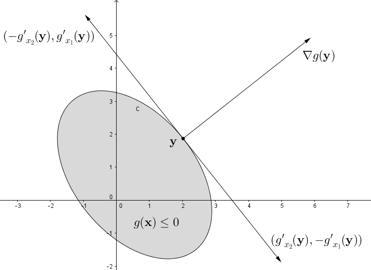
Figure 1: Tangent vectors

Definition 11

The positive (resp. negative) direction of moving along the curve $g(\vec{x})=0$ is the direction corresponding to the vector $(-g_{x_{2}}(\vec{x}),g_{x_{1}}(\vec{x}))$ (resp. $(g_{x_{2}}(\vec{x}),-g_{x_{1}}(\vec{x}))$).

Definition 12

wrede2010advanced Given a differentiable function $f$, the directional derivative of $f$ along vector $\vec{u}$ is defined as:

$$\frac{\partial f(\vec{x})}{\partial\vec{u}}=(\nabla f(\vec{x}))^{T}\cdot\vec{u}$$

Lemma 4

Consider differentiable functions $f:\mathbb{R}^{2}\rightarrow\mathbb{R}$ and $g:\mathbb{R}^{2}\rightarrow\mathbb{R}$. We have $\nabla f(\vec{y})\times\nabla g(\vec{y})\geq 0$ (resp. $\nabla f(\vec{y})\times\nabla g(\vec{y})\leq 0$) if and only if $f(\vec{x})$ is non-increasing (resp. non-decreasing) when moving along the curve $g(\vec{x})=0$ in the positive direction.

Proof

We will prove the case where $f$ is non-increasing.

Consider the directional derivative of $f$ with respect to the tangent vector at point $\vec{y}$:

$$\frac{\partial f}{\partial(-g^{\prime}_{x_{2}}(\vec{y}),g^{\prime}_{x_{1}}(\vec{y}))}(\vec{y})=(\nabla f(\vec{y}))\cdot(-g^{\prime}_{x_{2}}(\vec{y}),g^{\prime}_{x_{1}}(\vec{y}))^{T}=$$

$$-f^{\prime}_{x_{1}}(\vec{y})g^{\prime}_{x_{2}}(\vec{y})+f^{\prime}_{x_{2}}(\vec{y})g^{\prime}_{x_{1}}(\vec{y})=-\nabla f(\vec{y})\times\nabla g(\vec{y})\leq 0,$$

and this implies that the cross product being non-negative at $\vec{y}$ is equivalent to $f$ being non-increasing on $g(\vec{x})=0$ at $\vec{y}$.

∎

3.1 Reformulation of the KKT conditions

Now we shall establish a connection between the KKT conditions and the sign of the cross products corresponding to the gradient vectors.

Lemma 5

Consider a point $\vec{x}^{*}\in F$ with two active non-redundant constraints $g_{1}(\vec{x})\leq 0$ and $g_{2}(\vec{x})\leq 0$ such that $\nabla g_{1}(\vec{x}^{*})\times\nabla g_{2}(\vec{x}^{*})>0$. $\vec{x}^{*}$ is a KKT point if and only if

$$\nabla f(\vec{x}^{*})\times\nabla g_{1}(\vec{x}^{*})\geq 0,$$

$$\nabla f(\vec{x}^{*})\times\nabla g_{2}(\vec{x}^{*})\leq 0.$$

Proof

By KKT conditions (1)-(4), there exist $\mu_{1},\mu_{2}$ such that the following holds:

$$\begin{cases}\mu_{1}\frac{\partial g_{1}}{\partial x_{1}}(\vec{x}^{*})+\mu_{2}\frac{\partial g_{2}}{\partial x_{1}}(\vec{x}^{*})=\frac{\partial f}{\partial x_{1}}(\vec{x}^{*})\\[5.69054pt] \mu_{1}\frac{\partial g_{1}}{\partial x_{2}}(\vec{x}^{*})+\mu_{2}\frac{\partial g_{2}}{\partial x_{2}}(\vec{x}^{*})=\frac{\partial f}{\partial x_{2}}(\vec{x}^{*})\\[5.69054pt] \mu_{1},\mu_{2}\geq 0\end{cases}$$

From this system we can find $\mu_{1},\mu_{2}$:

$$\mu_{1}=\frac{\frac{\partial f}{\partial x_{1}}(\vec{x}^{*})\frac{\partial g_{2}}{\partial x_{2}}(\vec{x}^{*})-\frac{\partial g_{2}}{\partial x_{1}}(\vec{x}^{*})\frac{\partial f}{\partial x_{2}}(\vec{x}^{*})}{\frac{\partial g_{1}}{\partial x_{1}}(\vec{x}^{*})\frac{\partial g_{2}}{\partial x_{2}}(\vec{x}^{*})-\frac{\partial g_{2}}{\partial x_{1}}(\vec{x}^{*})\frac{\partial g_{1}}{\partial x_{2}}(\vec{x}^{*})}=\frac{\nabla f(\vec{x}^{*})\times\nabla g_{2}(\vec{x}^{*})}{\nabla g_{1}(\vec{x}^{*})\times\nabla g_{2}(\vec{x}^{*})}$$

$$\mu_{2}=\frac{\frac{\partial g_{1}}{\partial x_{1}}(\vec{x}^{*})\frac{\partial f}{\partial x_{2}}(\vec{x}^{*})-\frac{\partial f}{\partial x_{1}}(\vec{x}^{*})\frac{\partial g_{1}}{\partial x_{2}}(\vec{x}^{*})}{\frac{\partial g_{1}}{\partial x_{1}}(\vec{x}^{*})\frac{\partial g_{2}}{\partial x_{2}}(\vec{x}^{*})-\frac{\partial g_{2}}{\partial x_{1}}(\vec{x}^{*})\frac{\partial g_{1}}{\partial x_{2}}(\vec{x}^{*})}=\frac{\nabla g_{1}(\vec{x}^{*})\times\nabla f(\vec{x}^{*})}{\nabla g_{1}(\vec{x}^{*})\times\nabla g_{2}(\vec{x}^{*})}$$

$\mu_{1},\mu_{2}\geq 0$ is equivalent to

$$\nabla f(\vec{x}^{*})\times\nabla g_{1}(\vec{x}^{*})\geq 0$$

$$\nabla f(\vec{x}^{*})\times\nabla g_{2}(\vec{x}^{*})\leq 0$$

∎

4 Parametrization of the boundary of $F$

Given a real variable $t\in[0,T]$, where $T\in\mathbb{R},~{}T>0$, define a parametrization $\gamma:\mathbb{R}\rightarrow\mathbb{R}^{2}$ of $\partial F$ such that $\gamma(0)=\gamma(T)$ and the direction of increase of $t$ corresponds to the positive direction of moving along the boundary. Then

$$\gamma^{\prime}_{-}(t)=\left(-\frac{\partial g_{i^{-}(t)}}{\partial x_{2}}(\gamma(t)),\frac{\partial g_{i^{-}(t)}}{\partial x_{1}}(\gamma(t))\right)^{T}$$

$$\gamma^{\prime}_{+}(t)=\left(-\frac{\partial g_{i^{+}(t)}}{\partial x_{2}}(\gamma(t)),\frac{\partial g_{i^{+}(t)}}{\partial x_{1}}(\gamma(t))\right)^{T}$$

where $i^{-}(t)$ and $i^{+}(t)$ are indices of constraints that are active at $\gamma(t)$ and non-redundant in some neighborhood of this point. If there is only one active non-redundant constraint at $\gamma(t)$, then $i^{-}(t)=i^{+}(t)=i(t)$ and $\gamma^{\prime}_{-}(t)=\gamma^{\prime}_{+}(t)=\gamma^{\prime}(t)$. Otherwise we will require that there exists an $\epsilon_{0}>0$ such that $i^{-}(t)=i(t-\epsilon)$ and $i^{+}(t)=i(t+\epsilon)~{}\forall\epsilon\in(0,\epsilon_{0})$.

Let $\gamma^{r}(t)$ be the reversed direction parametrization of $\partial F$:

$$\gamma^{r\prime}_{-}(t)=\left(\frac{\partial g_{i^{r-}(t)}}{\partial x_{2}}(\gamma(t)),-\frac{\partial g_{i^{r-}(t)}}{\partial x_{1}}(\gamma(t))\right)^{T},$$

$$\gamma^{r\prime}_{+}(t)=\left(\frac{\partial g_{i^{r+}(t)}}{\partial x_{2}}(\gamma(t)),-\frac{\partial g_{i^{r+}(t)}}{\partial x_{1}}(\gamma(t))\right)^{T},$$

where $i^{r-}(t)$, $i^{r+}(t)$ are defined in a similar way to the indices in the direct parametrization.

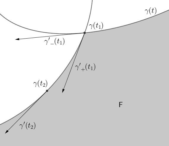
Figure 2: Parametrisation of the boundary of the feasible region

In the following Lemma, we show that $\gamma$ does not intersect itself.

Lemma 6

Consider two distinct values $t_{1}$ and $t_{2}$ of parameter $t$, such that $0<t_{1}<t_{2}<T$, then $\gamma(t_{1})\neq\gamma(t_{2})$.

Proof

We will proceed by contradiction, suppose that there exist numbers $t_{1}$, $t_{2}$ such that $\gamma(t_{1})=\gamma(t_{2})=\vec{y}$ and $0<t_{1}<t_{2}<T$. Let $j=i(t_{1})$ and $k=i(t_{2})$. Consider the product $(\nabla g_{j}(\vec{y}))^{T}\cdot\gamma^{\prime}(t_{2})$.

1. $(\nabla g_{j}(\vec{y}))^{T}\cdot\gamma^{\prime}(t_{2})=0$. Then

   $$(g_{j})^{\prime}_{x_{1}}(\vec{y})(g_{k})^{\prime}_{x_{2}}(\vec{y})-(g_{j})^{\prime}_{x_{2}}(\vec{y})(g_{k})^{\prime}_{x_{1}}(\vec{y})$$

   $$=(\nabla g_{j}(\vec{y}))^{T}\cdot((g_{k})^{\prime}_{x_{2}}(\vec{y}),-(g_{k})^{\prime}_{x_{1}}(\vec{y}))^{T}=(\nabla g_{j}(\vec{y}))^{T}\cdot\gamma^{\prime}(t_{2})=0$$

   and thus

   $$(g_{j})^{\prime}_{x_{2}}(\vec{y})=\frac{(g_{j})^{\prime}_{x_{1}}(\vec{y})(g_{k})^{\prime}_{x_{2}}(\vec{y})}{(g_{k})^{\prime}_{x_{1}}(\vec{y})}.$$

   If $c=-\frac{(g_{j})^{\prime}_{x_{1}}(\vec{y})}{(g_{k})^{\prime}_{x_{1}}(\vec{y})}$, we have that

   $$c\nabla g_{k}(\vec{y})=-\frac{(g_{j})^{\prime}_{x_{1}}(\vec{y})}{(g_{k})^{\prime}_{x_{1}}(\vec{y})}\left(\begin{array}[]{c}(g_{k})^{\prime}_{x_{1}}(\vec{y})\\[-5.69054pt] \\ (g_{k})^{\prime}_{x_{2}}(\vec{y})\\ \end{array}\right)=-\left(\begin{array}[]{c}(g_{j})^{\prime}_{x_{1}}(\vec{y})\\[-5.69054pt] \\ \frac{(g_{k})^{\prime}_{x_{2}}(\vec{y})(g_{j})^{\prime}_{x_{1}}(\vec{y})}{(g_{k})^{\prime}_{x_{1}}(\vec{y})}\\ \end{array}\right)$$

   $$=-\left(\begin{array}[]{c}(g_{j})^{\prime}_{x_{1}}(\vec{y})\\[-5.69054pt] \\ (g_{j})^{\prime}_{x_{2}}(\vec{y})\\ \end{array}\right)$$

   and

   $$\nabla g_{j}(\vec{y})+c\nabla g_{k}(\vec{y})=\nabla g_{j}(\vec{y})-\nabla g_{j}(\vec{y})=0.$$

   This violates LICQ.

2. $(\nabla g_{j}(\vec{y}))^{T}\cdot\gamma^{\prime}(t_{2})\neq 0$. This product can be interpreted as the directional derivative of $g_{j}$ with respect to $\gamma^{\prime}(t_{2})$. Note that $g_{j}(\vec{y})=0$. Since the directional derivative is non-zero and $\gamma^{\prime}(t_{2})$ locally approximates $\gamma(t)$, then $g_{j}$ changes sign on $\gamma(t)$ at $t_{2}$. Then we either have $g_{j}(\gamma(t_{2}-\epsilon))<0$ and $g_{j}(\gamma(t_{2}+\epsilon))>0$, or $g_{j}(\gamma(t_{2}-\epsilon))>0$. In both cases there exist infeasible points on $\gamma(t)$. But since $F$ is a closed set, $\partial F\in F$ and all points $\vec{x}=\gamma(t),~{}t\in[0,T]$ are feasible. Contradiction.

∎

Lemma 7

Consider a boundary point $\vec{y}=\gamma(t^{y})$. If there exist two constraints that are active and non-redundant at $\vec{y}$, then $\nabla g_{i^{-}(t^{y})}(\vec{y})\times\nabla g_{i^{+}(t^{y})}(\vec{y})>0$.

Proof

Consider the vector $\gamma_{+}^{\prime}(t^{y})$, which is the tangent vector to $g_{i^{+}(t^{y})}$ at point $\vec{y}$. By definition of $i^{+}$, constraint $g_{i^{+}(t^{y})}$ is active and non-redundant on $\gamma(t)$ in some right neighborhood of $t^{y}$. Then the tangent is a feasible direction at $\vec{y}$ with respect to constraint $g_{i^{-}(t^{y})}(\vec{x})\leq 0$. This can be written as:

$$(\nabla g_{i^{-}(t^{y})}(\vec{y}))^{T}\cdot\gamma_{+}^{\prime}(t^{y})\leq 0.$$

Or, equivalently:

$$\left(\frac{\partial g^{\prime}_{i^{-}(t^{y})}}{\partial x_{1}}(\vec{y}),\frac{\partial g^{\prime}_{i^{-}(t^{y})}}{\partial x_{2}}(\vec{y})\right)\cdot\left(-\frac{\partial g^{\prime}_{i^{+}(t^{y})}}{\partial x_{2}}(\vec{y}),\frac{g^{\prime}_{i^{+}(t^{y})}}{\partial x_{1}}(\vec{y})\right)^{T}\leq 0~{}\Leftrightarrow$$

$$-\left(\frac{\partial g^{\prime}_{i^{-}(t^{y})}}{\partial x_{1}}(\vec{y})\frac{\partial g^{\prime}_{i^{+}(t^{y})}}{\partial x_{2}}(\vec{y})-\frac{\partial g^{\prime}_{i^{-}(t^{y})}}{\partial x_{2}}(\vec{y})\frac{g^{\prime}_{i^{+}(t^{y})}}{\partial x_{1}}(\vec{y})\right)\leq 0~{}\Leftrightarrow$$

$$\left(\frac{\partial g^{\prime}_{i^{-}(t^{y})}}{\partial x_{1}}(\vec{y})\frac{\partial g^{\prime}_{i^{+}(t^{y})}}{\partial x_{2}}(\vec{y})-\frac{\partial g^{\prime}_{i^{-}(t^{y})}}{\partial x_{2}}(\vec{y})\frac{g^{\prime}_{i^{+}(t^{y})}}{\partial x_{1}}(\vec{y})\right)\geq 0~{}\Leftrightarrow$$

$$\nabla g_{i^{-}(t^{y})}(\vec{y})\times\nabla g_{i^{+}(t^{y})}(\vec{y})\geq 0.$$

If $\nabla g_{i^{-}(t^{y})}(\vec{y})\times\nabla g_{i^{+}(t^{y})}(\vec{y})=0$, then LICQ is violated at point $\vec{y}$:

$$\nabla g_{i^{-}(t^{y})}(\vec{y})+c\nabla g_{i^{+}(t^{y})}(\vec{y})=0\text{ if }c=\left(\frac{\partial g^{\prime}_{i^{-}(t^{y})}}{\partial x_{1}}(\vec{y})\right)/\left(\frac{\partial g^{\prime}_{i^{+}(t^{y})}}{\partial x_{1}}(\vec{y})\right).$$

Thus only strict inequality is possible:

$$\nabla g_{i^{-}(t^{y})}(\vec{y})\times\nabla g_{i^{+}(t^{y})}(\vec{y})>0.$$

∎

5 Splitting the space in two

5.1 Behavior of a concave function on a line

First we will prove a general result for one-dimensional real analytic functions.

Lemma 8

Let $f:\mathbb{R}\rightarrow\mathbb{R}$ be a real analytic function. If $f$ is constant on some nonempty interval $[a,b]$, then it is identically constant.

Proof

Suppose that $b$ is the largest number such that $f(x)$ is constant for all $x\in[a,b]$. Since $f$ is real analytic at $b$, at each point $\vec{y}$ the Taylor series $\sum\limits_{i=0}^{\infty}\frac{f^{(}n)(\vec{y})}{n!}(\vec{x}-\vec{y})$ converges to $f(\vec{y})$ krantz2002primer . $f$ being constant in some left neighborhood of $b$ implies that left-sided derivatives of any order are equal to $0$ at $b$. Then all coefficients of the Taylor series defining $f$ around $b$ are equal to $0$, so there exists $\epsilon>0$ such that $f(x)=0~{}\forall x\in(b-\epsilon),(b+\epsilon)$. But then $f$ is constant on $(a,b+\epsilon)$, which is impossible as $b+\epsilon>b$.

∎

Let $f:\mathbb{R}^{2}\rightarrow\mathbb{R}$ be a real analytic concave function. Consider a linear function $l(x_{1},x_{2})=ax_{1}+bx_{2}+c$. Let $\vec{y}$ be a point such that $l(\vec{y})=0$. We will define two rays:

Definition 13

$r^{d}(\vec{y})$ is the ray lying on the line $l(\vec{x})=0$ starting at $\vec{y}$ and pointing in the locally decreasing direction of $f$.

Definition 14

$r^{i}(\vec{y})$ is the ray lying on the line $l(\vec{x})=0$ starting at $\vec{y}$ and pointing in the locally increasing direction of $f$.

Let $\vec{x}^{max}_{l}$ be a point maximizing $f$ subject to $l(\vec{x})=0$.

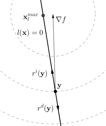
Figure 3: Rays $r^{i}(\vec{y})$ and $r^{d}(\vec{y})$

Lemma 9

If a concave real analytic function $f(\vec{x})$ is not identically constant on $l(\vec{x})=0$ then it is strictly decreasing on $r^{d}(\vec{y})$.

Proof

Consider two points $\vec{x}^{1},\vec{x}^{2}\in r^{d}(\vec{y})$ such that $||\vec{x}^{2}-\vec{y}||>||\vec{x}^{1}-\vec{y}||$. Since $f$ is locally decreasing at $\vec{y}$ in the direction of $r^{d}(\vec{y})$, $(f^{\prime}(\vec{y}))^{T}\cdot(\vec{x}^{1}-\vec{y})\leq 0$. By concavity of $f(\vec{x})$ we have:

$$f(\vec{x}^{1})-f(\vec{y})\leq(f(\vec{y}))^{T}\cdot(\vec{x}^{1}-\vec{y})~{}\Rightarrow~{}f(\vec{x}^{1})-f(\vec{y})\leq 0~{}\Rightarrow~{}f(\vec{y})-f(\vec{x}^{1})\geq 0.$$

Using the concavity of $f(\vec{x})$ again, we get:

$$f(\vec{y})-f(\vec{x}^{1})\leq(f(\vec{x}^{1}))^{T}\cdot(\vec{y}-\vec{x}^{1})~{}\Rightarrow~{}(f(\vec{x}^{1}))^{T}\cdot(\vec{y}-\vec{x}^{1})\geq 0$$

$$\Rightarrow~{}(f(\vec{x}^{1}))^{T}\cdot(\vec{x}^{2}-\vec{x}^{1})\leq 0.$$

Repeating the same reasoning for $\vec{x}^{1}$ and $\vec{x}^{2}$ as for $\vec{y}$ and $\vec{x}^{1}$, we can show that $f(\vec{x}^{2})\leq f(\vec{x}^{1})$.

Since $f(x_{1},x_{2})$ is real analytic, so is $f(x_{1},-\frac{ax_{1}+c}{b})$, which is the function of one variable $x_{1}$ and represents the behavior of $f$ on $l(\vec{x})=0$. Since $f(x_{1},-\frac{ax_{1}+c}{b})$ is not identically constant, by Lemma 8 no interval exists where it is constant. Then strict inequality holds: $f(\vec{x}^{2})<f(\vec{x}^{1})$.

∎

5.2 Boundary optimality on a half-plane

Let $\hat{\vec{x}}=\gamma(\hat{t})$ be a point on the boundary of $F$. In this section we will assume that for the parametrization $\gamma(t)$ defined in Section 4, $f(\gamma(t))$ is non-increasing as a function of $t$ on some interval $[\hat{t},\hat{t}+\epsilon]$, where $\epsilon>0$. Otherwise, similar results can be proven for the reverse direction parametrization $\gamma^{r}(t)$.

Definition 15

mendelson1990introduction A path in $\mathbb{R}^{n}$ is a continuous function mapping every point in the unit interval $[0,1]$ to a point in $\mathbb{R}^{n}$:

$$\rho:[0,1]\rightarrow\mathbb{R}^{n}$$

Consider a function $l:\mathbb{R}^{2}\rightarrow\mathbb{R}$ such that $l(\hat{\vec{x}})=0$. Let $t^{1}>\hat{t}$ be a parameter value corresponding to the point where $\gamma(t)$ first crosses the line $l(\vec{x})=0$ after $\hat{t}$:

$$t^{1}=\begin{cases}\min\{t>\hat{t}~{}|~{}l(\gamma(t))=0\}\text{ if such }t\text{ exist}\\ \infty\text{ otherwise }\end{cases}$$

$t^{1}$ exists if $F$ is bounded.

Define the optimization problem

max $$f(x_{1},x_{2})$$

s.t. $$g_{i}(x_{1},x_{2})\leq 0\text{ }\forall i=1..m$$ (NLP_l)

$$l(x_{1},x_{2})\leq 0$$

$$(x_{1},x_{2})\in\mathbb{R}^{2}.$$

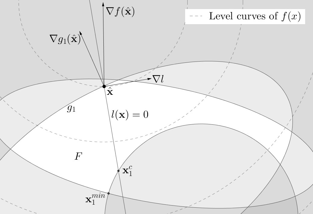
Figure 4: An example problem for Lemma 10

Lemma 10

Given $\gamma(t)$, a parametrization of $\partial F$ in (2.4) and given a linear function $l(\vec{x})$, if (2.4) is boundary-invex and $\hat{\vec{x}}$ is a KKT point of (5.2), then $f(\gamma(t))\leq f(\gamma(\hat{t}))~{}\forall t\in[\hat{t},t^{1}]$.

Proof

Let $t^{1}_{min}$ denote the parameter value corresponding to the point where $f(\gamma(t))$ starts increasing as a function of $t$:

$$\begin{cases}t^{1}_{min}>\hat{t}\\ (\nabla f(\gamma(t))\times\nabla g_{i(t)}(\gamma(t)))\geq 0~{}\forall t\in(\hat{t},t^{1}_{min})\\ (\nabla f(\gamma(t))\times\nabla g_{i(t)}(\gamma(t)))<0~{}\forall t\in(t^{1}_{min},t^{1}_{min}+\epsilon)\text{ for some }\epsilon>0\par\end{cases}$$

$t^{1}_{min}$ exists since $F$ is bounded. Let $\vec{x}_{min}^{1}=\gamma(t^{1}_{min})$.

If $t^{1}_{min}=t^{1}$, then for all $\hat{t}<t\leq t^{1}$ the inequality $f(\gamma(t))\leq f(\gamma(\hat{t}))$ is satisfied and the statement of the lemma holds. Now suppose that $t^{1}_{min}<t^{1}$.

Consider the set

$$L_{1}=\left\{\vec{x}~{}\left|~{}\begin{cases}l(\vec{x})\leq 0\\ f(\vec{x})\geq f(\vec{x}_{min}^{1})\end{cases}\right.\right\}$$

and the curve $\gamma_{1}(t)=\gamma(t),~{}t\in[\hat{t},t^{1}_{min})$. $F$ is connected, $\gamma_{1}(t)$ is piecewise-continuous, and $\gamma_{1}(\hat{t})=\hat{\vec{x}}$ lies on the line $l(\vec{x})=0$ and $\gamma_{1}(t^{1}_{min})$ lies on the curve $f(\vec{x})=f(\vec{x}_{min}^{1})$, and these are the only points of intersection of the curve and the boundary of $L_{1}$. Thus $\gamma_{1}(t)$ is dividing $L_{1}$ into two connected sets. We will denote the set where all points in the neighborhood of $\gamma_{1}(t)$ are feasible as $S_{1}$.

We know that, by definition of $S_{1}$, all points on its boundary belong to one of the following sets:

1. The level curve $f(\vec{x})=f(\vec{x}_{min}^{1})$. By definition of $\vec{x}_{min}^{1}$ we have that $f(\vec{x}_{min}^{1})\leq f(\hat{\vec{x}})$.

2. The curve $\gamma_{1}(t)$. By definition of $\gamma_{1}(t)$ and $t_{min}^{1}$, $f(\vec{x})\leq f(\hat{\vec{x}})~{}\forall\vec{x}\in\gamma_{1}(t)$.

3. The line $l(\vec{x})=0$. Since $\hat{\vec{x}}$ is a KKT point and thus, by Lemma 2, a local maximum, only the direction of local decrease of $f$ on the line is locally feasible. Together with the fact that $\hat{\vec{x}}$ is the only point where $\gamma_{1}(t)$ crosses the line, we have that points $\vec{x}$ in $S_{1}$ for which $l(\vec{x})=0$ lie on the ray $r^{d}(\hat{\vec{x}})$ and, by Lemma 9, satisfy $f(\vec{x})\leq f(\hat{\vec{x}})$.

Thus $f(\vec{x})\leq f(\hat{\vec{x}})~{}\forall\vec{x}\in\partial S_{1}$. By Lemma 2, $\hat{\vec{x}}$ is a local maximum in $S_{1}$ and thus, by Lemma 1, $f(\vec{x})\leq f(\hat{\vec{x}})~{}\forall\vec{x}\in S_{1}$.

The points following $\gamma(t^{1}_{min})$ are in $S_{1}$

We will say that a path $\rho$ starting at some point $\vec{x}^{s}\in\gamma_{1}(t)$ is $S_{1}$-feasible if $\vec{x}\in\rho\implies\vec{x}\in S_{1}$.

The definition of $S_{1}$ implies that for all constraints $g_{i}$ that are active on $\gamma_{1}(t)$, $g_{i}(\vec{x})<0$ for all $\vec{x}$ on $\rho$ in some neighborhood of $\vec{x}^{s}$ excluding $\vec{x}^{s}$ itself.

Consider a neighborhood $N(\vec{x}^{1}_{min})$ such that only constraints $g_{i^{-}(t^{1}_{min})}$ and $g_{i^{+}(t^{1}_{min})}$ are non-redundant in it.

Let $t^{-}=t^{1}_{min}-\epsilon$ and $t^{+}=t^{1}_{min}+\epsilon$ for some $\epsilon>0$ and let:

$$\vec{x}^{-}=\gamma(t^{-}),~{}\vec{x}^{+}=\gamma(t^{+}),$$

$$\phi^{-}=g_{i^{-}(t_{min}^{1})},~{}\phi^{+}=g_{i^{+}(t_{min}^{1})}.$$

We will show that there exists an $\epsilon_{0}$ such that for all $\epsilon<\epsilon_{0}$ the segment connecting $\gamma(t^{-})$ and $\gamma(t^{+})$ satisfies the conditions defined for the path $\rho$.

Consider two cases:

1. One constraint is active at $\vec{x}_{min}^{1}$.

   Define $\phi=\phi^{-}=\phi^{+}$.

   In this case $\vec{x}^{1}_{min}$ is a local minimum of $f$ on $\phi(\vec{x})=0$. Then $\phi$ is either concave or convex in some neighborhood $N(\vec{x}^{1}_{min})$. If $\phi$ is concave in $N(\vec{x}^{1}_{min})$, then $\vec{x}^{1}_{min}$ violates boundary-invexity of (2.4). Indeed, this point is a KKT point for (NLP_2i) with a negative KKT multiplier and not a local maximum for (2.4).

   Then $\phi$ can only be convex in $N(\vec{x}^{1}_{min})$.

   Since $\vec{x}^{+}$ is feasible and belongs to the neighborhood of $\vec{x}^{1}_{min}$, then $\phi(\vec{x})\leq 0~{}\forall\vec{x}\in\overline{\vec{x}^{-}\vec{x}^{+}}$ and $\phi(\vec{x})<0$ for all $\vec{x}$ on this segment excluding $\vec{x}^{-}$. Hence $\vec{x}^{+}\in S_{1}$.

2. Two constraints are active at $\vec{x}_{min}^{1}$.

   By Lemma 7, $\nabla\phi^{-}(\vec{x}_{min}^{1})\times\nabla\phi^{+}(\vec{x}^{1}_{min})>0$. By definitions of the two-dimensional cross product, this is equivalent to:

   $$(\nabla\phi^{-}(\vec{x}^{1}_{min}))^{T}\cdot\gamma^{\prime}_{+}(t^{1}_{min})<0$$

   This product can be interpreted as the directional derivative of $\phi^{-}$ with respect to the vector $\gamma^{\prime}_{+}$. Observe that $\gamma^{\prime}_{+}(t^{1}_{min})$ shows how $\vec{x}$ behaves on $\gamma(t)$ when small changes to $t$ are made. Therefore, the above inequality implies that there exists $\epsilon_{0}$ such that for any $\epsilon<\epsilon_{0}$ the following holds:

   $$(\nabla\phi^{-}(\vec{x}^{1}_{min}))^{T}\cdot(\vec{x}^{+}-\vec{x}^{1}_{min})<0$$

   Since all constraints are twice continuously differentiable, $\nabla\phi^{-}(\vec{x})(\vec{x}^{+}-\vec{x})$ is a differentiable function of $\vec{x}$. Thus there exists a neighborhood $N(\vec{x}^{1}_{min})$ where this function stays negative. We can choose $\epsilon_{0}$ such that $\vec{x}^{-}\in N(\vec{x}^{1}_{min})~{}\forall\epsilon<0$ and:

   $$(\nabla\phi^{-}(\vec{x}^{-}))^{T}\cdot(\vec{x}^{+}-\vec{x}^{-})<0$$

   There exists $\epsilon_{0}$ such that $\phi^{-}(\vec{x})\leq 0~{}\forall\vec{x}\in\overline{\vec{x}^{-}\vec{x}^{+}}$ if $\epsilon<\epsilon_{0}$. Thus the segment $\overline{\vec{x}^{-}\vec{x}^{+}}$ is an $S_{1}$-feasible path.

Exiting $S_{1}$

By Lemma 6, $\gamma(t)$ cannot intersect itself and therefore cannot cross $\gamma_{1}(t)$. Consequently, there are only two ways of exiting $S_{1}$:

1. Crossing the level curve. Then $f$ is decreasing on $\gamma(t)$ at the intersection point. Let the next point where $f(\gamma(t))$ starts increasing again be denoted as $t^{2}_{min}$ and define $\gamma_{2}(t)=\gamma(t),~{}t\in[\hat{t},t^{2}_{min}]$. This curve has the same properties as $\gamma_{1}(t)$:

   1. $f(\vec{x})\leq f(\hat{\vec{x}})$ for all $\vec{x}$ on $\gamma_{2}(t)$ and

   2. $\gamma_{2}(t)$ only crosses the line $l(\vec{x})=0$ at $\hat{\vec{x}}$ and the level curve $f(\vec{x})=f(\vec{x}^{2}_{min})$ at $\vec{x}^{2}_{min}$, where $\vec{x}^{2}_{min}=\gamma(t^{2}_{min})$.

   Then $S_{2}$ can be defined similarly to $S_{1}$ with the new parameters and the same reasoning can be repeated.

2. Cross $l(\vec{x})=0$. Then $f(\gamma(t))\leq f(\gamma(\hat{t}))~{}\forall t\in[\hat{t},t^{1}]$.

∎

Lemma 11

Consider a point $\hat{\vec{x}}$ satisfying the conditions of Lemma 10 with $l(\vec{x})$ and $\gamma(t)$. Let $\vec{x}^{1}\in r^{i}(\hat{\vec{x}})$ be the next point where $\gamma(t)$ crosses the line after $\hat{\vec{x}}$, then $\vec{x}^{1}$ satisfies the conditions of Lemma 10 for $\gamma(t)$ and $-l(\vec{x})$.

Proof

Let $t^{1}$ be defined similarly to Lemma 10 and $\vec{x}^{1}=\gamma(t^{1})$.

It follows immediately from the definition of $\vec{x}^{1}$ that $l(\vec{x}^{1})=0$.

First let us prove that $f(\gamma(t))$ is non-increasing as a function of $t$ at $t^{1}$. Assume the contrary: $f(\gamma(t))$ strictly increases as a function of $t$ at $t^{1}$. Then there exists a $t^{i}_{min}$ such that $\hat{t}<t_{min}^{i}<t^{1}$ and $f(\gamma(t))$ is monotone on the $[t^{i}_{min},t^{1}]$ interval.

Then there exists a set $S_{i}$ and, as proved in the previous lemma, if $\vec{x}\in r^{i}(\hat{\vec{x}})$ then $\vec{x}\notin S_{i}$. Then $\gamma(t)$ has to exit $S_{i}$ at some $t<t^{1}$. There are two possibilities:

1. $\gamma(t)$ crosses $r^{d}(\hat{\vec{x}})$. This contradicts with $\gamma(t^{1})\in r^{i}(\hat{\vec{x}})$,

2. $\gamma(t)$ crosses the level curve. Then $f(\gamma(t))$ decreases somewhere between $t_{min}^{1}$ and $t^{1}$. This contradicts with $f(\gamma(t))$ being monotonic on $[t^{i}_{min},t^{1}]$.

This proves that $f(\gamma(t))$ is non-increasing at $t^{1}$.
Now we shall show that $x^{1}$ is a local maximizer of $f$ in $F\cap l(\vec{x})\geq 0$.
By Lemma 4, $f(\gamma(t))$ being non-increasing at $t^{1}$ implies that:

$$\nabla f(\vec{x}^{1})\times\nabla g_{i(t^{1})}(\vec{x}^{1})\geq 0.$$ (5)

Since $\gamma(t)$ crosses the line from the $l(\vec{x})\leq 0$ half-space into the $l(\vec{x})\geq 0$ half-space at $\vec{x}^{1}$ , $l(\gamma(t))$ is increasing at $t^{1}$ and thus, by Lemma 4, we have that $\nabla l\times\nabla g_{i(t^{1})}(\vec{x}^{1})\leq 0$ or, equivalently:

$$(-\nabla l)\times\nabla g_{i(t^{1})}(\vec{x}^{1})>0.$$ (6)

Finally, by Lemma 10, $f(\vec{x}^{1})\leq f(\hat{\vec{x}})$ and thus $\vec{x}^{1}$ belongs to the part of ray $r^{i}(\hat{\vec{x}})$ where $f$ is decreasing. If we consider the direction which $r^{i}(\hat{\vec{x}})$ points to as the positive direction of moving along the line, then the corresponding gradient is $-\nabla l$. Then Lemma 4 implies that

$$\nabla f(\vec{x}^{1})\times(-\nabla l)\geq 0.$$ (7)

By Lemma 5, these inequalities imply that $\vec{x}^{1}$ is a KKT point in $F\cap\{l(\vec{x})\geq 0\}$. Thus the conditions of Lemma 10 are satisfied at $\vec{x}^{1}$ for $F\cap\{l(\vec{x})\geq 0\}$.

∎

6 Kuhn-Tucker invexity of boundary-invex problems

6.1 Sequence of crossing points

Consider a point $\vec{x}^{*}$ which is a local maximum of (2.4) and a linear function $l(\vec{x})$ such that $f$ is not constant on $l(\vec{x})=0$. Let $\gamma(0)=\vec{x}^{*}$.

Given two parameter values $r,s$, let $\hat{\gamma}(r,s)$ denote the segment of the $\gamma(t)$ curve with $t\in[r,s]$.

Let $\vec{x}^{i}$ be the $i^{th}$ point where $\gamma(t)$ crosses $l(\vec{x})=0$ and let $t^{i}$ be a parameter value such that $\vec{x}^{i}=\gamma(t^{i})$. Since $\gamma(t)$ is a closed curve, $\vec{x}^{i}$ exists for each $i\in\mathbb{N}$ if at least one crossing point exists.

The numbering of the crossing points will be chosen so that the even indices will correspond to $\gamma(t)$ crossing the line $l(\vec{x})=0$ from $l(\vec{x})>0$ into $l(\vec{x})<0$, and the odd indices will correspond to the opposite direction of crossing.

Lemma 12

Consider a crossing point $\vec{x}^{i}$, $i\in 2\mathbb{N}$. If $\nabla l\times\nabla f(\vec{x}^{i})\geq 0$, then $\vec{x}^{i}$ satisfies Lemma 10 for either $l(\vec{x})$ and $\gamma(t)$ or for $-l(\vec{x})$ and $\gamma^{r}(t)$.

Proof

Since $\gamma(t)$ crosses the line from $l(\vec{x})<0$ into $l(\vec{x})>0$ at $\vec{x}^{i}$, we have that $\nabla l\times\nabla g_{i(t^{i})}(\vec{x}^{i})<0$.

By Lemma 5, $\vec{x}^{i}$ is a KKT point in one of the following sets:

1. $F\cap\{l(\vec{x})\leq 0\}$ if $\nabla f\times\nabla g_{i(t^{i})}\geq 0$. The latter inequality also implies that Lemma 10 is satisfied at $\vec{x}^{i}$ for $\gamma(t)$ and $l(\vec{x})$ (see the beginning of Section 5).

2. $F\cap\{-l(\vec{x})\leq 0\}$ if $\nabla f\times\nabla g_{i(t^{i})}\leq 0$. The latter inequality implies that Lemma 10 is satisfied at $\vec{x}^{i}$ for $\gamma^{r}(t)$ and $-l(\vec{x})$.

∎

Let $S(\overline{AB},\overline{BC},...)\subset F$ denote a set with the boundary comprised of some sections of $\partial F$ and segments $\overline{AB}$, $\overline{BC}$, $...$ on the line $l(\vec{x}=0)$.

Definition 16

$S(\overline{AB},\overline{BC},...)\subset F$ is a safe set if $f(\vec{x})\leq f(\vec{x}^{*})~{}\forall\vec{x}\in S$.

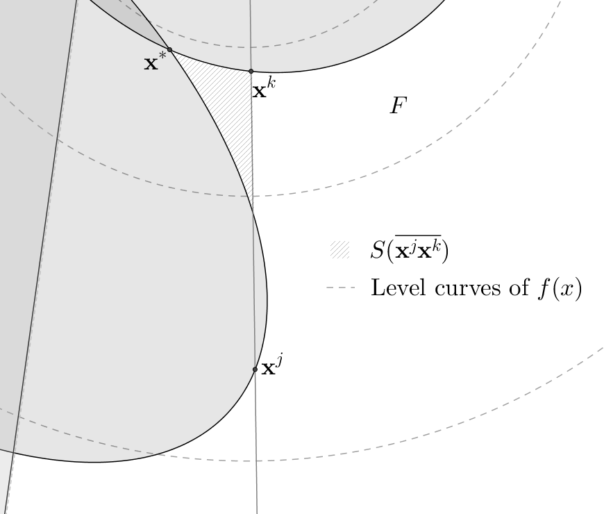
Figure 5: Points $\vec{x}^{*}$, $\vec{x}^{j}$, $\vec{x}^{k}$ and set $S(\overline{\vec{x}^{j}\vec{x}^{k}})$ satisfying the conditions of Theorem 6.1

Theorem 6.1

Consider points $\vec{x}^{j}$, $\vec{x}^{k}\in F$ such that:

$\vec{x}^{k},~{}k\in 2\mathbb{N}$, satisfies Lemma 10 for $\gamma^{r}$ and $-l$, $f(\vec{x}^{k})\leq f(\vec{x}^{*})$;

$\vec{x}^{j}\in r^{d}(\vec{x}^{k}),~{}j\in 2\mathbb{N}$, satisfies Lemma 10 for $\gamma$ and $l$;

$f(\gamma(t))<f(\vec{x}^{*})~{}\forall t\in[0,t^{j}]$;

if $\vec{x}^{j}\neq\vec{x}^{k}$ and $\gamma(t)$ crosses $\overline{\vec{x}^{j}\vec{x}^{k}}$ from $l(\vec{x})>0$ into $l(\vec{x})<0$, it enters a safe set $S(\overline{\vec{x}^{j}\vec{x}^{k}})$ with the boundary consisting of $\overline{\vec{x}^{j}\vec{x}^{k}}$ and $\hat{\gamma}(t^{k},t^{j-1})$.

Then $x^{*}$ is the global optimum of (2.4).

Proof

The conditions on $\vec{x}^{k}$ imply that $\nabla f(\vec{x}^{k})\times\nabla l\leq 0$. By Lemma 9, $f$ is monotonically decreasing on the whole ray $r^{d}(\vec{x}^{k})$ and thus $\nabla f(\vec{x})\times\nabla l\leq 0~{}\forall\vec{x}\in r^{d}(\vec{x}^{k})$. Then points $\vec{x}^{i}\in r^{d}(\vec{x}^{k}),~{}i\in 2\mathbb{N}$, satisfy conditions of Lemma 12.

Let us consider the following cases:

1. $\vec{x}^{j+1}\in r^{d}(\vec{x}^{k})$.
   

   Let $S(\overline{\vec{x}^{j}\vec{x}^{j+1}})$ be the set with the boundary composed of $\hat{\gamma}(t^{j},t^{j+1})$ and the segment $\overline{\vec{x}^{j}\vec{x}^{j+1}}$. By Lemma 10, $f(\vec{x})\leq f(\vec{x}^{j})~{}\forall\vec{x}\in\hat{\gamma}(t^{j},t^{j+1})$. Since the segment $\overline{\vec{x}^{j}\vec{x}^{j+1}}$ is part of the $r^{d}(\vec{x}^{j})$ ray, then by Lemma 9, $f$ is decreasing on this segment from $x^{j}$ in the direction of $x^{j+1}$ and thus $f(\vec{x})\leq f(\vec{x}^{j})~{}\forall\vec{x}\in\overline{\vec{x}^{j}\vec{x}^{j+1}}$. Since $\vec{x}^{j}$ satisfies the conditions of Lemma 10, it is a local maximum in $S(\overline{\vec{x}^{j}\vec{x}^{j+1}})$. Then, by Lemma 1, $f(\vec{x})\leq f(\vec{x}^{j})\leq f(\vec{x}^{*})~{}\forall\vec{x}\in S(\overline{\vec{x}^{j}\vec{x}^{j+1}})$. Thus $S(\overline{\vec{x}^{j}\vec{x}^{j+1}})$ is a safe set.
   

   By Lemma 6, $\gamma(t)$ cannot exit $S(\overline{\vec{x}^{j}\vec{x}^{j+1}})$ by crossing itself. Then the only way to exit $S(\overline{\vec{x}^{j}\vec{x}^{j+1}})$ is to cross the $\overline{\vec{x}_{j}\vec{x}_{j+1}}$ line segment again.
   

   Let $S(\overline{\vec{x}^{j}\vec{x}^{k}},\overline{\vec{x}^{j}\vec{x}^{j+1}})=S(\overline{\vec{x}^{j}\vec{x}^{k}})\cup S(\overline{\vec{x}^{j}\vec{x}^{j+1}})$. Since it is a union of two safe sets, $S(\overline{\vec{x}^{j}\vec{x}^{k}},\overline{\vec{x}^{j}\vec{x}^{j+1}})$ is a safe set.
   

   If $\vec{x}^{j+2}=\vec{x}^{k}$, then, by Lemma 10 applied to $x^{k}$, $-l$ and $\gamma^{r}$, $f(\vec{x})\leq f(\vec{x}^{k})\leq f(\vec{x}^{*})~{}\forall\vec{x}\in\hat{\gamma}(t^{j+1},t^{j+2})$. Since the conditions of the theorem imply that $f(\gamma(t))\leq f(\vec{x}^{*})~{}\forall t\in[k,T]\cup[0,j]$, we have that $f(\gamma(t))\leq f(\vec{x}^{*})~{}\forall t\in[0,T]$.
   

   We will consider the following cases that depend on the position of $\vec{x}^{j+2}$ on $l(\vec{x})=0$:
   

   1. $\vec{x}^{j+2}\in\overline{\vec{x}^{k}\vec{x}^{j+1}}$.
      

      $\gamma(t)$ enters $S(\overline{\vec{x}^{j}\vec{x}^{k}},\overline{\vec{x}^{j}\vec{x}^{j+1}})$ at $\vec{x}^{j+2}$. Since it is a safe set, $f$ cannot reach values larger than $f(\vec{x}^{*})$ unless $\vec{x}^{j+3}$ exists. Repeat case (1) with $\vec{x}^{j+3}$ instead of $\vec{x}^{j+1}$.
      

   2. $\vec{x}^{j+2}\in r^{d}(\vec{x}^{j+1})$.
      

      $j{+}2\in 2\mathbb{N}$. Since $\vec{x}^{j+2}\in r^{d}(\vec{x}^{j+1})\in r^{d}(\vec{x}^{k})$ and, by Lemma 9, a concave function is always decreasing in the direction of local decrease from a given point, the monotonicity of $f$ on $l(\vec{x})=0$ at $\vec{x}^{j+2}$ is similar to that at $\vec{x}^{k}$. This implies that $sign(\nabla l\times\nabla f(\vec{x}^{j+2}))=sign(\nabla l\times\nabla f(\vec{x}^{k}))\geq 0$. Then, by Lemma 12, one of the following is true at $\vec{x}^{j+2}$:

      1. $f(\gamma(t))$ is increasing at $t^{j+2}$. Then at this point Lemma 10 can be applied for $\gamma^{r}$ and $-l$ to show that $f(\gamma(t))\leq f(\vec{x}^{j+2})~{}\forall t\in(t^{j+1},t^{j+2})$. But by Lemma 9, $f$ is non-increasing on $r^{d}(\vec{x}^{k})$ and $f(\vec{x}^{j+2})<f(\vec{x}^{j+1})$. This contradicts with $f(\vec{x}^{j+2})\leq f(\vec{x}^{j+1})$.

      2. $f(\gamma(t))$ is decreasing at $t^{j+2}$. Then Lemma 10 is satisfied at $\vec{x}^{j+2}$ for $\gamma$ and $l$. Then $\vec{x}^{j+2},\vec{x}^{k}$ and the $l(\vec{x})=0$ line satisfy the conditions of this theorem and the reasoning can be repeated from the start.

   3. $\vec{x}^{j+2}\in r^{i}(\vec{x}^{k})$.
      

      

      Figure 6: Case (1c): $\vec{x}^{j+1}\in r^{d}(\vec{x}^{k})$

      Let $S(\overline{\vec{x}^{j+1}\vec{x}^{j+2}})$ be the set with the boundary composed of $\overline{\vec{x}^{j+1}\vec{x}^{j+2}}$ and $\gamma(t^{j+1},t^{j+2})$. Let $S(\overline{\vec{x}^{j+2}\vec{x}^{k}})=S(\overline{\vec{x}^{j+1}\vec{x}^{j+2}})$ $\cup S(\overline{\vec{x}^{k}\vec{x}^{j}})$ $\cup S(\overline{\vec{x}^{j}\vec{x}^{j+1}})$.
      

      At $\vec{x}^{j+2}$ $\gamma(t)$ leaves $S(\overline{\vec{x}^{j+2}\vec{x}^{k}})$. But $\vec{x}^{k}$ belongs to the boundary of $S(\overline{\vec{x}^{j+2}\vec{x}^{k}})$ and $\gamma(t)$ approaches $\vec{x}^{k}$ from the interior of this set. This implies that at some point $\gamma(t)$ enters $S(\overline{\vec{x}^{j+2}\vec{x}^{k}})$. Let $\vec{x}^{m}$ denote the last such point on $\gamma(t)$ before $x^{k}$. Then the next crossing point $\vec{x}^{m+1}$ can only belong to $\overline{\vec{x}^{k}\vec{x}^{j+1}}$.
      

      $f(\gamma(t))$ is increasing at $t^{m}$
      

      Consider the point $\vec{x}^{k-1}$. If $\vec{x}^{k-1}=\vec{x}^{m}$, then the proof is done.
      

      Now suppose that $\vec{x}^{k-1}\neq\vec{x}^{m}$. The definition of $\vec{x}^{m}$ implies that $\vec{x}^{k-1}\in\overline{\vec{x}^{k}\vec{x}^{j+1}}$. The points following $\vec{x}^{k-1}$ on $\gamma^{r}(t)$ belong to one of the sets $S(\overline{\vec{x}^{k}\vec{x}^{j}})$, $S(\overline{\vec{x}^{j}\vec{x}^{j+1}})$. Thus $f(\gamma(t))\leq f(\vec{x}^{*})~{}\forall t\in[k-1,k]$ and $\vec{x}^{k-2}$ exists and belongs to $\overline{x^{k}x^{j+1}}$. Consider the following cases:
      

      1. $\vec{x}^{k-2}\in\overline{\vec{x}^{k}\vec{x}^{k-1}}$. Then $\gamma^{r}(t)$ enters the set $S(\overline{\vec{x}^{k}\vec{x}^{k-1}})$ and $\vec{x}^{k-3}\neq x^{m}$. Repeat case (1ci) with $\vec{x}^{k-3}$ instead of $\vec{x}^{k-1}$.
         

      2. $\vec{x}^{k-2}\in\overline{\vec{x}^{k-1}\vec{x}^{j-1}}$. Then, similarly to case (1b), $\vec{x}^{k-2}$ satisfies the conditions of Lemma 10 for $-l$ and $\gamma^{r}$. Thus $f(\gamma(t))\leq f(\vec{x}^{*})~{}\forall t\in[t^{k-2},t^{k-3}]$. If $\vec{x}^{k-3}=\vec{x}^{m}$, by Lemma 11 $\vec{x}^{m}$ satisfies the conditions of Lemma 10 for $l$ and $\gamma$. Otherwise repeat (1ci) and (1cii) with $\vec{x}^{k-2}$ instead of $\vec{x}^{k}$ and $\vec{x}^{k-3}$ instead of $\vec{x}^{k-1}$.
         

      We have proven that $f(\gamma(t))\leq f(\vec{x}^{*})~{}\forall t\in[t^{k},t^{m}]$ and $\vec{x}^{m}$ satisfies the conditions of Lemma 10 for $l$ and $\gamma$.
      

      Starting a new iteration
      

      Consider the set $S(\overline{\vec{x}^{j+2}\vec{x}^{m}})$ that contains the section of the $\gamma(t)$ curve from $t^{m}$ to $t^{j+2}$. If this set is disconnected, then there exist points $\vec{x}\in S(\overline{\vec{x}^{j+2}\vec{x}^{m}})$ that cannot be connected to the segment $\overline{\vec{x}^{j+2}\vec{x}^{m}}$ by a continuous path that belongs to this set. But since every feasible path from $S(\overline{\vec{x}^{j+2}\vec{x}^{m}})$ to $F\setminus S(\overline{\vec{x}^{j+2}\vec{x}^{m}})$ crosses $\overline{\vec{x}^{j+2}\vec{x}^{m}}$, this implies that there is no feasible path from $\vec{x}$ to points in $F\setminus S(\overline{\vec{x}^{j+2}\vec{x}^{m}})$ and thus $F$ is disconnected. This contradicts with the theorem assumptions. Hence $S(\overline{\vec{x}^{j+2}\vec{x}^{m}})$ is a connected set.
      

      We have shown that $f(\vec{x})\leq f(\vec{x}^{*})$ for all $\vec{x}$ on this curve. $\vec{x}^{*}$ is a local maximum in $S(\overline{\vec{x}^{j+2}\vec{x}^{m}})$. Then $f(\vec{x})\leq f(\vec{x}^{*})~{}\forall\vec{x}\in S(\overline{\vec{x}^{j+2}\vec{x}^{m}})$.
      

      Case (1) of this theorem can be repeated with $\vec{x}^{j+2}$, $S(\overline{\vec{x}^{j+2}\vec{x}^{m}})$, $-l$ and $\vec{x}^{m}$ instead of $\vec{x}^{j+1}$, $S(\overline{\vec{x}^{j}\vec{x}^{k}},\overline{\vec{x}^{j}\vec{x}^{j+1}})$, $l$ and $\vec{x}^{k}$.
      

   

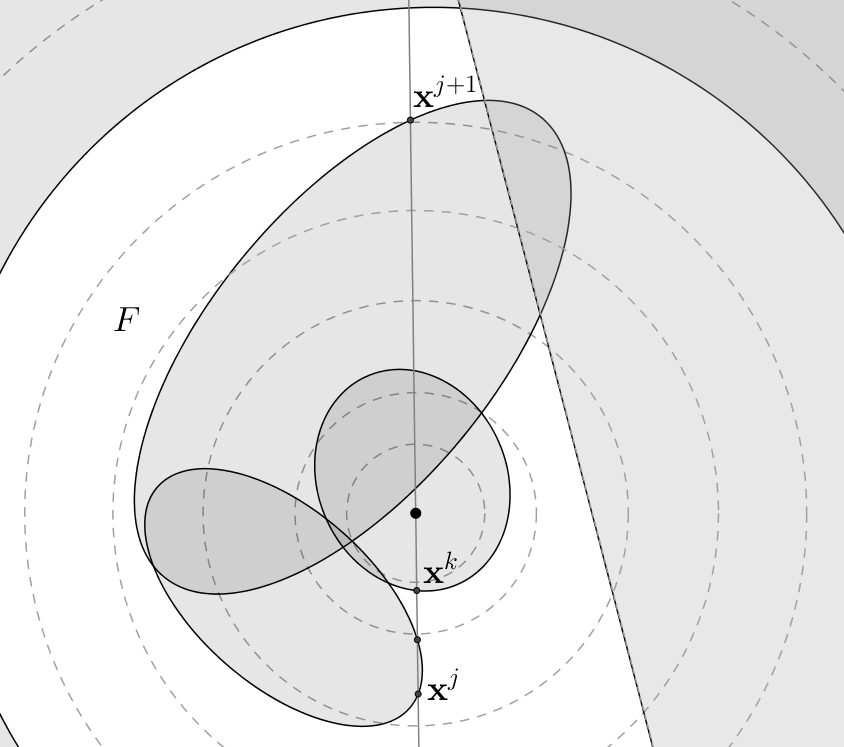
   Figure 7: Case 2: $\vec{x}^{j+1}\in r^{i}(\vec{x}^{k})$

2. $\vec{x}^{j+1}\in r^{i}(\vec{x}^{k})$. By Lemma 11, $f(\gamma(t))$ is decreasing at $t^{j+1}$ and $\vec{x}^{j+1}$ satisfies the conditions of Lemma 10. Then $f(\vec{x})\leq f(\vec{x}^{j+1})$ until the next crossing point $\vec{x}^{j+2}$.

   1. $\vec{x}^{j+2}\in\overline{\vec{x}^{k}\vec{x}^{j+1}}$.

      The assumptions of this theorem imply that $f(\vec{x}^{k})>f(\vec{x}_{j})\geq f(\vec{x}^{j+1})$. This means that $\vec{x}^{k}$ belongs to the increasing section of the ray $r^{i}(\vec{x}^{j+1})$ and $f(\vec{x})>f(\vec{x}^{j+1})~{}\forall\vec{x}\in\overline{\vec{x}^{k}\vec{x}^{j+1}}$. Then $f(\vec{x}^{j+2})>f(\vec{x}^{j+1})$. Contradiction with $f(\vec{x}^{j+2})\leq f(\vec{x}^{j+1})$.
      

   2. $\vec{x}^{j+2}\in r^{d}(\vec{x}^{k})$.

      By applying Lemma 11 to $\vec{x}^{j+2}$ we can show that this point satisfies the conditions of Lemma 10 for $\gamma$ and $l$. Then $\vec{x}^{j+2}$ has the same properties as $\vec{x}^{j}$. Repeat everything with same $\vec{x}^{k}$ and $\vec{x}^{j+2}$ instead of $\vec{x}^{j}$.
      

   3. $\vec{x}^{j+2}\in r^{d}(\vec{x}^{j+1})$.

      1. $\vec{x}^{j+3}\in r^{d}(\vec{x}^{j+2})$. Repeat (2) with $\vec{x}^{j+3}$ instead of $\vec{x}^{j+1}$.

      2. $\vec{x}^{j+3}\in\overline{\vec{x}^{k}\vec{x}^{j+2}}$. From $\vec{x}^{j+2}$ $\gamma(t)$ cannot reach the line segment $\overline{\vec{x}^{k}\vec{x}_{j+1}}$ without crossing $\hat{\gamma}(t^{j},t^{j+1})$. Then $\vec{x}^{j+2}\in\overline{\vec{x}^{j+1}\vec{x}^{j+2}}$ and $\gamma(t)$ enters a safe set $S(\overline{\vec{x}^{j+1}\vec{x}^{j+2}})$. Then $\vec{x}^{j+4}\in\overline{\vec{x}^{j+1}\vec{x}^{j+2}}$. Repeat (2c) with $\vec{x}^{j+4}$ instead of $\vec{x}^{j+2}$.

      3. $\vec{x}^{j+3}\in r^{d}(\vec{x}^{k})$. Repeat (1) with $\vec{x}^{j+3}$ instead of $\vec{x}^{j+1}$.

We have proven that $f(\gamma(t))\leq f(\vec{x}^{*})~{}\forall t\in[0,T]$. By Lemma 1, together with the fact that $\vec{x}^{*}$ is a local maximum this implies that $\vec{x}^{*}$ is the global maximum of (2.4).

∎

6.2 The main theorem

Theorem 6.2

If (2.4) is boundary-invex, then it is KT-invex.

Proof

Let $\vec{x}^{*}$ be a KKT point. If $\vec{x}^{*}$ lies in the interior of $F$, then, by concavity of $f$, it is the global unconstrained maximum of $f$ and thus the global maximum for (2.4).

Now suppose that $\vec{x}^{*}\in\partial F$. Let $\gamma(0)=\gamma(T)=\vec{x}^{*}$ in the parametrization of $\partial F$. By Lemma 1, it is enough to consider only the values on the boundary. We need to prove that there exists a line $l(\vec{x})=0$ such that the conditions of Theorem 6.1 are satisfied for the point $\vec{x}^{*}=\vec{x}_{j}=\vec{x}_{k}$.

If $\nabla g_{1}(\vec{x}^{*})\times\nabla g_{2}(\vec{x}^{*})=0$, then $\nabla g_{1}(\vec{x}^{*})=c\nabla g_{2}(\vec{x}^{*})$, and LICQ is violated. Now suppose that $\nabla g_{1}(\vec{x}^{*})\times\nabla g_{2}(\vec{x}^{*})\neq 0$. Since $\vec{u}\times\vec{v}=-(\vec{v}\times\vec{u})$, we can assume w.l.o.g. that $\nabla g_{1}(\vec{x}^{*})\times\nabla g_{2}(\vec{x}^{*})<0$. Then, by Lemma 5, the following holds:

$$\nabla f(\vec{x}^{*})\times\nabla g_{1}(\vec{x}^{*})\geq 0$$ (8)

$$\nabla f(\vec{x}^{*})\times\nabla g_{2}(\vec{x}^{*})\leq 0$$ (9)

Consider a linear function $l(x_{1},x_{2})$ such that $l(\vec{x}^{*})=0$ and $\nabla l=-\nabla g_{1}(\vec{x}^{*})+\nabla g_{2}(\vec{x}^{*})$. By (8), (9) we have:

$$\nabla f(\vec{x}^{*})\times\nabla l=-\nabla f(\vec{x}^{*})\times\nabla g_{1}(\vec{x}^{*})+\nabla f(\vec{x}^{*})\times\nabla g_{2}(\vec{x}^{*})<0$$

and

$$\nabla l\times\nabla g_{1}(\vec{x}^{*})=-\nabla g_{1}(\vec{x}^{*})\times\nabla g_{1}(\vec{x}^{*})+\nabla g_{2}(\vec{x}^{*})\times\nabla g_{1}(\vec{x}^{*})=$$

$$\nabla g_{2}(\vec{x}^{*})\times\nabla g_{1}(\vec{x}^{*})>0,$$

$$\nabla l\times\nabla g_{2}(\vec{x}^{*})=-\nabla g_{1}(\vec{x}^{*})\times\nabla g_{2}(\vec{x}^{*})+\nabla g_{2}(\vec{x}^{*})\times\nabla g_{2}(\vec{x}^{*})=$$

$$-\nabla g_{1}(\vec{x}^{*})\times\nabla g_{2}(\vec{x}^{*})>0.$$

By Lemma 5, these inequalities imply that $\vec{x}^{*}$ is a KKT point in both $F\cap\{l(\vec{x})\leq 0\}$ and $F\cap\{l(\vec{x})\geq 0\}$. $\nabla f(\vec{x}^{*})\times\nabla l<0$ also implies that $f$ is non-constant on $l(\vec{x})=0$. Theorem 6.1 can then be applied to show that $\vec{x}^{*}$ is the global maximum of (2.4).

∎

7 Application

Notations

$\bm{i}$ - imaginary number constant

$S=p+\bm{i}q$ - Electric power

$V=v\angle\theta$ - Voltage

$\bm{Y}=\bm{g}+\bm{i}\bm{b}$ - Line admittance

$W\!=w^{R}\!+\bm{i}w^{I}$ - Product of two voltages

$\bm{s}^{u}$ - Line apparent power thermal limit

$\theta_{ij}$ - Phase angle difference (i.e., $\theta_{i}-\theta_{j}$)

$\bm{S}^{d}=\bm{p}^{d}+\bm{i}\bm{q}^{d}$ - Power demand

$S^{g}=p^{g}+\bm{i}q^{g}$ - Power generation

$\bm{c}_{0},\bm{c}_{1},\bm{c}_{2}$ - Generation cost coefficients

$\Re(\cdot)$ - Real part of a complex number

$\Im(\cdot)$ - Imaginary part of a complex number

$(\cdot)^{*}$ - Conjugate of a complex number

$|\cdot|$ - Magnitude of a complex number, $l^{2}$-norm

$\bm{x}^{l},\bm{x}^{u}$ - Lower and upper bounds of $x$

7.1 The Power Flow Equations

In Power Systems, the Alternating Current (AC) power flow equations link the complex quantities of voltage $V$, power $S$, and admittance $Y$, using Ohm’s and Kirchhoff’s Current Laws. They can be written as,

$$S^{g}_{i}-{\bm{S}^{d}_{i}}=\sum_{\begin{subarray}{c}(i,j)\in E\end{subarray}}S_{ij}+\sum_{\begin{subarray}{c}(j,i)\in E\end{subarray}}S_{ij}\;\;\forall i\in N$$ (10a)

$$S_{ij}=\bm{Y}^{*}_{ij}V_{i}V^{*}_{i}-\bm{Y}^{*}_{ij}V_{i}V^{*}_{j}\;\;(i,j),(j,i)\in E$$ (10b)

A detailed derivation of these equations can be found in qc_opf_tps . The non-convex nonlinear equations (10a)–(10b) form the core building block of many power network optimization applications. These equations are usually augmented with side constraints such as,

$$\Re(\bm{S^{gl}}_{i})\leq\Re(S^{g}_{i})\leq\Re(\bm{S^{gu}}_{i})\;\;\forall i\in N$$ (11)

$$\Im(\bm{S^{gl}}_{i})\leq\Im(S^{g}_{i})\leq\Im(\bm{S^{gu}}_{i})\;\;\forall i\in N$$ (12)

$$(\bm{v^{l}}_{i})^{2}\leq|V_{i}|^{2}\leq(\bm{v^{u}}_{i})^{2}\;\;\forall i\in N$$ (13)

$$|S_{ij}|\leq\bm{s^{u}}_{ij}\;\;\forall(i,j),(j,i)\in E$$ (14)

$$\tan(\bm{\theta^{l}}_{ij})\Re(V_{i}V^{*}_{j})\!\leq\!\Im(V_{i}V^{*}_{j})\!\leq\!\tan(\bm{\theta^{u}}_{ij})\Re(V_{i}V^{*}_{j})\;\forall(i,j)\!\in\!E.$$ (15)

Constraints (11)–(12) set limits on the real and reactive generator capabilities, respectively. Constraints (13) limit the magnitudes of bus voltages. Constraints (14) limit the power flow on the lines and constraints (15) limit the difference of the phase angles (i.e., $\theta_{i},\theta_{j}$) between the lines’ buses. A detailed derivation and further explanation of these operational side constraints can be found in qc_opf_tps .

7.2 Optimal Power Flow

Model 1 The AC Optimal Power Flow Problem (AC-OPF).

variables:

$$S^{g}_{i}\in(\bm{S^{gl}}_{i},\bm{S^{gu}}_{i})\;\;\forall i\in N$$

$$V_{i}\in(\bm{V^{l}}_{i},\bm{V^{u}}_{i})\;\;\forall i\in N$$

$$W_{ij}\in(\bm{W^{l}}_{ij},\bm{W^{u}}_{ij})\;\;\forall i\in N,\forall j\in N$$

$$S_{ij}\in(\bm{S^{l}}_{ij},\bm{S^{u}}_{ij})\;\;\forall(i,j),(j,i)\in E$$

minimize:

$$\sum_{i\in N}\bm{c}_{2i}(\Re(S^{g}_{i}))^{2}+\bm{c}_{1i}\Re(S^{g}_{i})+\bm{c}_{0i}$$ (16a)

subject to:

$$\angle V_{\bm{r}}=0$$ (16b)

$$W_{ij}=V_{i}V_{j}^{*}\;\;\forall(i,j)\in E$$ (16c)

$$S^{g}_{i}-{\bm{S}^{d}_{i}}=\sum_{\begin{subarray}{c}(i,j)\in E\end{subarray}}S_{ij}+\sum_{\begin{subarray}{c}(j,i)\in E\end{subarray}}S_{ij}\;\;\forall i\in N$$ (16d)

$$S_{ij}=\bm{Y}^{*}_{ij}W_{ii}-\bm{Y}^{*}_{ij}W_{ij}\;\;\forall(i,j)\in E$$ (16e)

$$S_{ji}=\bm{Y}^{*}_{ij}W_{jj}-\bm{Y}^{*}_{ij}W_{ij}^{*}\;\;\forall(i,j)\in E$$ (16f)

$$|S_{ij}|\leq(\bm{s^{u}}_{ij})\;\;\forall(i,j),(j,i)\in E$$ (16g)

$$\tan(\bm{\theta^{l}}_{ij})\Re(W_{ij})\!\leq\!\Im(W_{ij})\!\leq\!\tan(\bm{\theta^{u}}_{ij})\Re(W_{ij})\;\forall(i,j)\!\in\!E$$

The AC Optimal Power Flow Problem (ACOPF) combines the above power flow equations, side constraints, and a convex objective function as described in Model 1. This formulation utilizes a voltage product factorization $V_{i}V_{j}^{*}=W_{ij}\;\;\forall(i,j)\in E$. Model 1 is a non-convex nonlinear optimization problem, which has been shown to be NP-Hard in general verma2009power ; ACSTAR2015 . In real-world deployments, the AC-OPF problem is solved with numerical methods such as 744492 ; 744495 , which are not guaranteed to converge to a feasible point and provide only stationary points (e.g., saddle points or local minimas) when convergence is achieved.

In the following section we look at a family of ACOPF problems with two degrees of freedom and show that they are boundary-invex under mild assumptions on the variables’ bounds. Namely, we will enforce that

$$-\frac{\pi}{6}\leq\bm{\theta}^{l}<\bm{\theta}^{u}\leq\frac{\pi}{6}\text{ and }0.95\leq\bm{v^{l}}_{i}<\bm{v^{u}}_{i}\leq 1.05.$$

7.3 Boundary-invex ACOPF

Model 2 AC-OPF for 1-line networks.

variables:

$$w^{R},~{}w^{I}$$

minimize:

$$\bm{c}_{1}(\bm{g}\bm{w}-\bm{g}w^{R}-\bm{b}w^{I})+\bm{c}_{2}(\frac{\bm{g}}{\bm{w}}((w^{R})^{2}+(w^{I})^{2})-\bm{g}w^{R}+\bm{b}w^{I})$$ (17a)

subject to:

$$(\bm{g}\bm{w}-\bm{g}w^{R}-\bm{b}w^{I})^{2}+(-\bm{b}\bm{w}+\bm{b}w^{R}-\bm{g}w^{I})^{2}\leq\bm{s}^{u}$$ (17b)

$$(\frac{\bm{g}}{\bm{w}}((w^{R})^{2}+(w^{I})^{2})-\bm{g}w^{R}+\bm{b}w^{I})^{2}$$

$$+(-\frac{\bm{b}}{\bm{w}}((w^{R})^{2}+(w^{I})^{2})+\bm{b}w^{R}+\bm{g}w^{I})^{2}\leq\bm{s}^{u}$$ (17c)

$$(\bm{p}_{1}^{g})^{l}-\bm{p}_{1}^{d}\leq\bm{g}\bm{w}-\bm{g}w^{R}-\bm{b}w^{I}\leq(\bm{p}_{1}^{g})^{u}-\bm{p}_{1}^{d}$$ (17d)

$$(\bm{q}_{1}^{g})^{l}-\bm{q}_{1}^{d}\leq-\bm{b}\bm{w}+\bm{b}w^{R}-\bm{g}w^{I}\leq(\bm{q}_{1}^{g})^{u}-\bm{q}_{1}^{d}$$ (17e)

$$(\bm{p}_{2}^{g})^{l}-\bm{p}_{2}^{d}\leq\frac{\bm{g}}{\bm{w}}((w^{R})^{2}+(w^{I})^{2})-\bm{g}w^{R}+\bm{b}w^{I}\leq(\bm{p}_{2}^{g})^{u}-\bm{p}_{2}^{d}$$ (17f)

$$(\bm{q}_{2}^{g})^{l}-\bm{q}_{2}^{d}\leq-\frac{\bm{b}}{\bm{w}}((w^{R})^{2}+(w^{I})^{2})+\bm{b}w^{R}+\bm{g}w^{I}\leq(\bm{q}_{2}^{g})^{u}-\bm{q}_{2}^{d}$$ (17g)

$$(\bm{v^{l}}_{2})^{2}\leq\frac{(w^{R})^{2}+(w^{I})^{2}}{\bm{w}}\leq(\bm{v^{u}}_{2})^{2}$$ (17h)

$$w^{R}\tan(\bm{\theta}^{l})\leq w^{I}\leq w^{R}\tan(\bm{\theta}^{u})$$ (17i)

Figure 8: 1-line network

Consider a 2-bus network with one line and two generators as depicted in Figure 8. We assume the voltage magnitude to be fixed at node $1$. For clarity purposes we will adopt the following notations: $\bm{w}=\bm{w}_{1}$, $w^{R}=w^{R}_{12}$, $w^{I}=w^{I}_{12}$ and $\bm{s}^{u}=\bm{s}^{u}_{12}$. The real-number formulation of Model 1 is given in Model 2.

This model has four non-convex constraints, namely, (17c), (17f), (17g) and (17h).

Figure 9: Feasible set of Model 2 (feasible region in white)

Minimal feasible $w^{R}$

Lemma 13

If $w^{R}\leq 0.77\bm{w}$, then $(w^{R},w^{I})$ is infeasible for Model 2.

Proof

Consider the lower bound on $w_{2}$ and voltage angle bounds. No feasible points exist where:

$$w^{R}\tan(\bm{\theta}^{l})\leq w^{I}\leq w^{R}\tan(\bm{\theta}^{u})\implies(w^{R})^{2}+(w^{I})^{2}<(\bm{v^{l}}_{2})^{2}\bm{w}$$

If $w^{R}\geq(\bm{v^{l}}_{2})^{2}\bm{w}$, the latter is always false. Suppose that $w^{R}<(\bm{v^{l}}_{2})^{2}\bm{w}$. Consider the $w^{I}\geq 0$ half-space. The lower angle bound is redundant here, and the remaining two inequalities can be written as:

$$w^{I}\leq w^{R}\tan(\bm{\theta}^{u})$$

$$w^{I}<\sqrt{(\bm{v^{l}}_{2})^{2}\bm{w}-(w^{R})^{2}}$$

The implication holds if the second inequality is dominated by the first:

$$w^{R}\tan(\bm{\theta}^{u})<\sqrt{(\bm{v^{l}}_{2})^{2}\bm{w}-(w^{R})^{2}}\Leftrightarrow$$

$$(w^{R})^{2}\tan^{2}(\bm{\theta}^{u})<(\bm{v^{l}}_{2})^{2}\bm{w}-(w^{R})^{2}$$

It can be seen that only points with non-negative $w^{R}$ can satisfy constraint (17i). Then the above is equivalent to:

$$w^{R}<\sqrt{\frac{(\bm{v^{l}}_{2})^{2}\bm{w}}{\tan^{2}(\bm{\theta}^{u})+1}}.$$

Since $\bm{\theta}^{u}\leq\frac{\pi}{6}$ and $(\bm{v^{l}}_{2})^{2}\geq(0.95)^{2}$, we have that:

$$\sqrt{\frac{(\bm{v^{l}}_{2})^{2}\bm{w}}{\tan^{2}(\bm{\theta}^{u})+1}}\geq\sqrt{\frac{(0.95)^{2}\bm{w}}{\frac{1}{3}+1}}\geq 0.82\sqrt{\bm{w}}$$

All $w^{R}<0.82\sqrt{\bm{w}}$ are guaranteed to be infeasible. Since $\bm{w}\leq 1.1025$, it can be shown that $\sqrt{\bm{w}}\geq 0.95\bm{w}$ and thus all $w^{R}<0.77\bm{w}$ are infeasible.

∎

$w_{2}$ lower bound

Consider constraint (17h). Let $g_{1}(w^{R},w^{I})=(\bm{v^{l}})^{2}-\frac{(w^{R})^{2}+(w^{I})^{2}}{\bm{w}}$.

Lemma 14

KKT points of problem (NLP_2i), $i=1$ do not violate the boundary-invexity for Model 2.

Proof

(NLP_2i) takes the following form for $i=1$:

$$\max~{}c_{1}(\bm{g}\bm{w}-\bm{g}w^{R}-\bm{b}w^{I})+c_{2}(\frac{\bm{g}}{\bm{w}}((w^{R})^{2}+(w^{I})^{2})-\bm{g}w^{R}+\bm{b}w^{I})$$

$$s.t.~{}(w^{R})^{2}+(w^{R})^{2}=(\bm{v^{l}})^{2}\bm{w}$$

which can be rewritten as

$$\max~{}\bm{c}_{1}(\bm{g}\bm{w}-\bm{g}w^{R}-\bm{b}w^{I})+\bm{c}_{2}(\frac{\bm{g}}{\bm{w}}(\bm{v^{l}})^{2}\bm{w}-\bm{g}w^{R}+\bm{b}w^{I})$$

$$s.t.~{}(w^{R})^{2}+(w^{I})^{2}=(\bm{v^{l}})^{2}\bm{w}$$

The KKT conditions for this problem are:

$$-\bm{g}(\bm{c}_{1}+\bm{c}_{2})=2\lambda\hat{w}^{R}$$ (18)

$$\bm{b}(\bm{c}_{2}-\bm{c}_{1})=2\lambda\hat{w}^{I}$$ (19)

$$((\hat{w}^{R})^{2}+(\hat{w}^{I})^{2}=(\bm{v^{l}})^{2}\bm{w}$$ (20)

The solution of this system can violate boundary-invexity only if $\lambda>0$. It can be seen from (18) that $\hat{w}^{R}<0$ if $\lambda>0$. But since by Lemma 13 all points $(w^{R},w^{I})$ such that $w^{R}<0.77\bm{w}$ are infeasible, $(\hat{w}^{R},\hat{w}^{I})$ is infeasible.

∎

$p_{21}$ lower bound

Consider constraint (17f). Let $g_{2}=(\bm{p}_{2}^{g})^{l}-\bm{p}_{2}^{d}-\frac{\bm{g}}{\bm{w}}((w^{R})^{2}+(w^{I})^{2})+\bm{g}w^{R}-\bm{b}w^{I}$.

Lemma 15

KKT points of problem (NLP_2i), $i=2$ do not violate the boundary-invexity for Model 2.

Proof

(NLP_2i) takes the following form for $i=2$:

$$\max~{}\bm{c}_{1}(\bm{g}\bm{w}-\bm{g}w^{R}-\bm{b}w^{I})+\bm{c}_{2}(\frac{\bm{g}}{\bm{w}}((w^{R})^{2}+(w^{I})^{2})-\bm{g}w^{R}+\bm{b}w^{I})$$

$$s.t.~{}\frac{\bm{g}}{\bm{w}}((w^{R})^{2}+(w^{I})^{2})=(\bm{p}_{2}^{g})^{l}-\bm{p}_{2}^{d}+\bm{g}w^{R}-\bm{b}w^{I}$$

which can be rewritten as

$$\max~{}\bm{c}_{1}(\bm{g}\bm{w}-\bm{g}w^{R}-\bm{b}w^{I})+\bm{c}_{2}((\bm{p}_{2}^{g})^{l}-\bm{p}_{2}^{d})$$

$$s.t.~{}\frac{\bm{g}}{\bm{w}}((w^{R})^{2}+(w^{I})^{2})=(\bm{p}_{2}^{g})^{l}-\bm{p}_{2}^{d}+\bm{g}w^{R}-\bm{b}w^{I}$$

The KKT conditions for this problem are:

$$\bm{c}_{1}\bm{g} =-\lambda(\frac{2\bm{g}\hat{w}^{R}}{\bm{w}}-\bm{g})$$

$$\bm{c}_{1}\bm{b} =-\lambda(\frac{2\bm{g}\hat{w}^{I}}{\bm{w}}+\bm{b})$$

$$~{}\frac{\bm{g}}{\bm{w}}((\hat{w}^{R})^{2}+(\hat{w}^{I})^{2}) =(\bm{p}_{2}^{g})^{l}-\bm{p}_{2}^{d}+\bm{g}\hat{w}^{R}-\bm{b}\hat{w}^{I}$$

and the first equation implies that

$$\hat{w}^{R}=-\frac{\bm{c}_{1}\bm{w}}{2\lambda}+\frac{\bm{w}}{2}.$$

The solution of this system can violate boundary-invexity only if $\lambda>0$. Then $\hat{w}^{R}<\frac{\bm{w}}{2}$. But since by Lemma 13 all points $(w^{R},w^{I})$ such that $w^{R}<0.77\bm{w}$ are infeasible, $(\hat{w}^{R},\hat{w}^{I})$ is infeasible.

∎

$q_{21}$ lower bound

Consider constraint (17g). Let $g_{3}=(\bm{q}_{2}^{g})^{l}-\bm{q}_{2}^{d}+\frac{\bm{b}}{\bm{w}}((w^{R})^{2}+(w^{I})^{2})-\bm{b}w^{R}-\bm{g}w^{I}$.

Lemma 16

KKT points of problem (NLP_2i), $i=3$ do not violate the boundary-invexity for Model 2.

Proof

(NLP_2i) takes the following form for $i=3$:

$$\max~{}\bm{c}_{1}(\bm{g}\bm{w}-\bm{g}w^{R}-\bm{b}w^{I})+c_{2}(\frac{\bm{g}}{\bm{w}}((w^{R})^{2}+(w^{I})^{2})-\bm{g}w^{R}+\bm{b}w^{I})$$

$$s.t.~{}-\frac{\bm{b}}{\bm{w}}((w^{R})^{2}+(w^{I})^{2})=(\bm{q}_{2}^{g})^{l}-\bm{q}_{2}^{d}-\bm{b}w^{R}-\bm{g}w^{I}$$

which can be rewritten as

$$\max~{}\bm{c}_{1}(\bm{g}w-\bm{g}w^{R}-\bm{b}w^{I})+\frac{\bm{c}_{2}}{\bm{b}}((\bm{b}^{2}+\bm{g}^{2})w^{I}-\bm{g}((\bm{q}_{2}^{g})^{l}-\bm{q}_{2}^{d}))$$

$$s.t.~{}\frac{(w^{R})^{2}+(w^{I})^{2}}{\bm{w}}=-\frac{(\bm{q}_{2}^{g})^{l}-\bm{q}_{2}^{d}}{\bm{b}}+w^{R}+\frac{\bm{g}}{\bm{b}}w^{I}$$

The KKT conditions for this problem are:

$$\bm{c}_{1}\bm{g} =-\lambda(\frac{2\hat{w}^{R}}{\bm{w}}-1)$$

$$-\bm{c}_{1}\bm{b}-\frac{\bm{c}_{2}(\bm{b}^{2}+\bm{g}^{2})}{\bm{b}} =-\lambda(\frac{2\hat{w}^{I}}{\bm{w}}-\frac{\bm{g}}{\bm{b}})$$

$$~{}\frac{(\hat{w}^{R})^{2}+(\hat{w}^{I})^{2}}{\bm{w}} =-\frac{(\bm{q}_{2}^{g})^{l}-\bm{q}_{2}^{d}}{\bm{b}}+\hat{w}^{R}+\frac{\bm{g}}{\bm{b}}\hat{w}^{I}$$

and the first equation implies that

$$\hat{w}^{R}=-\frac{\bm{c}_{1}\bm{g}\bm{w}}{2\lambda}+\frac{\bm{w}}{2}.$$

The solution of this system can violate boundary-invexity only if $\lambda>0$. Then $\hat{w}^{R}<\frac{\bm{w}}{2}$. But since by Lemma 13 all points $(w^{R},w^{I})$ such that $w^{R}<0.77\bm{w}$ are infeasible, $(\hat{w}^{R},\hat{w}^{I})$ is infeasible.

∎

We now consider the thermal limit constraint (17c).

Lemma 17

If constraint (17c) is non-redundant in a given subset, it is locally convex in this subset.

Proof

Consider the boundary of the set defined by constraint (17c). It is given by:

$$(\frac{\bm{g}}{\bm{w}}((w^{R})^{2}+(w^{I})^{2})-\bm{g}w^{R}+\bm{b}w^{I})^{2}+(-\frac{\bm{b}}{\bm{w}}((w^{R})^{2}+(w^{I})^{2})+\bm{b}w^{R}+\bm{g}w^{I})^{2}$$

$$-\bm{s}^{u}=\frac{\bm{g}^{2}}{\bm{w}^{2}}s^{2}+\frac{2\bm{g}}{\bm{w}}s(\bm{b}w^{I}-\bm{g}w^{R})+(\bm{b}w^{I}-\bm{g}w^{R})^{2}+\frac{\bm{b}^{2}}{\bm{w}^{2}}s^{2}-\frac{2\bm{b}}{\bm{w}}s(\bm{b}w^{R}+\bm{g}w^{I})$$

$$+(\bm{b}w^{R}+\bm{g}w^{I})^{2}-\bm{s}^{u}=\frac{|\bm{Y}|}{\bm{w}^{2}}s^{2}+\frac{2}{\bm{w}}s(-\bm{g}^{2}w^{R}-\bm{b}^{2}w^{R})+(\bm{b}w^{I}-\bm{g}w^{R})^{2}$$

$$+(\bm{b}w^{R}+\bm{g}w^{I})^{2}-\bm{s}^{u}=\frac{|\bm{Y}|}{\bm{w}^{2}}s^{2}-\frac{2w^{R}|\bm{Y}|}{\bm{w}}s+|\bm{Y}|s-\bm{s}^{u}=0$$

where $s=(w^{R})^{2}+(w^{I})^{2}$ and $|\bm{Y}|=\bm{g}^{2}+\bm{b}^{2}$. This equation has the following solutions:

$$s=\frac{\bm{w}}{2}(2w^{R}-\bm{w}-\sqrt{(2w^{R}-\bm{w})^{2}+\frac{4\bm{s}^{u}}{|\bm{Y}|}})\text{ and}$$

$$s=\frac{\bm{w}}{2}(2w^{R}-\bm{w}+\sqrt{(2w^{R}-\bm{w})^{2}+\frac{4\bm{s}^{u}}{|\bm{Y}|}})$$

The first equation has no solution since $s$ is non-negative and the right-hand side is negative. Now we can write the thermal limit constraint as:

$$(w^{I})^{2}\leq\frac{\bm{w}}{2}(2w^{R}-\bm{w}+\sqrt{(2w^{R}-\bm{w})^{2}+\frac{4\bm{s}^{u}}{|\bm{Y}|}})-(w^{R})^{2}$$

Let $R=\sqrt{(2w^{R}-\bm{w})^{2}+\frac{4\bm{s}^{u}}{|\bm{Y}|}}$ and $\phi(w^{R})=\frac{\bm{w}}{2}(2w^{R}-\bm{w}+R)-(w^{R})^{2}$. Constraint (17c) describes a convex set if $\phi(w^{R})$ is concave. To obtain the conditions for its concavity, we will calculate the second derivative:

$$\phi^{\prime}(w^{R})=\frac{\bm{w}}{2}(2+R^{\prime})-2w^{R}$$

$$\phi^{\prime\prime}(w^{R})=\frac{\bm{w}}{2}R^{\prime\prime}-2=\frac{\bm{w}}{2}\frac{4R-\frac{4(2w^{R}-\bm{w})^{2}}{R}}{R^{2}}-2$$

A function is concave if its second derivative is negative:

$$\frac{\bm{w}}{2}\frac{4R-\frac{4(2w^{R}-\bm{w})^{2}}{R}}{R^{2}}-2<0$$

$$R^{2}-(2w^{R}-\bm{w})^{2}<\frac{R^{3}}{\bm{w}}$$

Observe that, from the definition of $R$, the left hand side of this inequality is equal to $\frac{4\bm{s}^{u}}{|\bm{Y}|}$:

$$\frac{4\bm{s}^{u}}{|\bm{Y}|}<\frac{R^{3}}{\bm{w}}~{}\Leftrightarrow~{}(\frac{4\bm{s}^{u}\bm{w}}{|\bm{Y}|})^{\frac{2}{3}}<R^{2}~{}\Leftrightarrow~{}$$

$$\sqrt[3]{(\frac{4\bm{s}^{u}\bm{w}}{|\bm{Y}|})^{2}}<(2w^{R}-\bm{w})^{2}+\frac{4\bm{s}^{u}}{|\bm{Y}|}~{}\Leftrightarrow~{}$$

$$w^{R}>\frac{1}{2}\sqrt{\sqrt[3]{(\frac{4\bm{s}^{u}\bm{w}}{|\bm{Y}|})^{2}}-\frac{4\bm{s}^{u}}{|\bm{Y}|}}+\frac{\bm{w}}{2}$$

Let $\psi(x)=x^{\frac{2}{3}}\bm{w}^{\frac{2}{3}}-x$. Find the stationary point of $\psi(x)$:

$$\psi^{\prime}(x)=\bm{w}^{\frac{2}{3}}\frac{2}{3}\frac{1}{\sqrt[3]{x}}-1=0$$

$$x=\frac{8\bm{w}^{2}}{27}$$

To verify the second order optimality condition, calculate the second derivative:

$$\psi^{\prime\prime}(x)=-\frac{2}{9}\bm{w}^{\frac{2}{3}}\frac{1}{\sqrt{x^{4}}}<0$$

Hence $\psi(x)$ is concave and

$$\psi(\frac{8\bm{w}^{2}}{27})=(\frac{8\bm{w}^{2}}{27})^{\frac{2}{3}}\bm{w}^{\frac{2}{3}}-\frac{8\bm{w}^{2}}{27}=\frac{4\bm{w}^{2}}{27}.$$

We have shown that $\psi(x)\leq\frac{4\bm{w}^{2}}{27}~{}\forall x>0$. Then we can guarantee that constraint (17c) is convex if

$$w^{R}>\bm{w}(\frac{1}{3\sqrt{3}}+0.5).$$

Since $(\frac{1}{3\sqrt{3}}+0.5)<0.77$ and, by Lemma 13, all $(w^{R},w^{I})$ such that $w^{R}<0.77\bm{w}$ are infeasible, (17c) is convex everywhere where it is non-redundant.

∎

Corollary 1

Model 2 is boundary-invex.

Proof

Based on Lemmas 14-17, we can show that all KKT points for the auxiliary NLP_2i problems are infeasible with respect to Model 2. Based on Definition 7, boundary-invexity is established.

∎

8 Conclusion

Given a non-convex optimization problem, boundary-invexity captures the behavior of the objective function on the boundary of its feasible region. In this work, we show that boundary-invexity is a necessary condition for KT-invexity, that becomes sufficient in the two-dimensional case. Unlike conventional invexity conditions, boundary-invexity can be verified algorithmically and in some cases in polynomial-time. This is a first step in extending the reach of interior-point methods to non-convex problems. Future research directions include extending the sufficiency proof to the n-dimensional case and deriving conditions for checking the connectivity of non-convex sets.

References

- (1) E. Abbena, S. Salamon, and A. Gray, Modern differential geometry of curves and surfaces with Mathematica, CRC press, 2006.
- (2) T. Antczak, (p, r)-invex sets and functions, Journal of Mathematical Analysis and Applications, 263 (2001), pp. 355–379.
- (3) C. Bector and C. Singh, B-vex functions, Journal of Optimization Theory and Applications, 71 (1991), pp. 237–253.
- (4) A. Ben-Israel and B. Mond, What is invexity?, The ANZIAM Journal, 28 (1986), pp. 1–9.
- (5) S. Boyd and L. Vandenberghe, Convex optimization, Cambridge university press, 2004.
- (6) C. Coffrin, H. L. Hijazi, and P. V. Hentenryck, The QC relaxation: A theoretical and computational study on optimal power flow, IEEE Transactions on Power Systems, 31 (2016), pp. 3008–3018, http://dx.doi.org/10.1109/TPWRS.2015.2463111.
- (7) B. Craven, Invex functions and constrained local minima, Bulletin of the Australian Mathematical society, 24 (1981), pp. 357–366.
- (8) B. Craven and B. Glover, Invex functions and duality, Journal of the Australian Mathematical Society (Series A), 39 (1985), pp. 1–20.
- (9) M. A. Hanson, On sufficiency of the kuhn-tucker conditions, Journal of Mathematical Analysis and Applications, 80 (1981), pp. 545–550.
- (10) V. Jeyakumar and B. Mond, On generalised convex mathematical programming, The Journal of the Australian Mathematical Society. Series B. Applied Mathematics, 34 (1992), pp. 43–53.
- (11) S. G. Krantz and H. R. Parks, A primer of real analytic functions, Springer Science & Business Media, 2002.
- (12) K. Lehmann, A. Grastien, and P. V. Hentenryck, Ac-feasibility on tree networks is np-hard, IEEE Transactions on Power Systems, 31 (2016), pp. 798–801, http://dx.doi.org/10.1109/TPWRS.2015.2407363.
- (13) O. L. Mangasarian, Pseudo-convex functions, Journal of the Society for Industrial and Applied Mathematics, Series A: Control, 3 (1965), pp. 281–290.
- (14) D. Martin, The essence of invexity, Journal of optimization Theory and Applications, 47 (1985), pp. 65–76.
- (15) B. Mendelson, Introduction to topology, Courier Corporation, 1990.
- (16) J. Momoh, R. Adapa, and M. El-Hawary, A review of selected optimal power flow literature to 1993. i. nonlinear and quadratic programming approaches, IEEE Transactions on Power Systems, 14 (1999), pp. 96 –104, http://dx.doi.org/10.1109/59.744492.
- (17) J. Momoh, M. El-Hawary, and R. Adapa, A review of selected optimal power flow literature to 1993. ii. newton, linear programming and interior point methods, IEEE Transactions on Power Systems, 14 (1999), pp. 105 –111, http://dx.doi.org/10.1109/59.744495.
- (18) Y. Nesterov and A. Nemirovskii, Interior-point polynomial algorithms in convex programming, SIAM, 1994.
- (19) P. M. Pardalos and G. Schnitger, Checking local optimality in constrained quadratic programming is np-hard, Operations Research Letters, 7 (1988), pp. 33–35.
- (20) G. F. Simmons, Introduction to topology and modern analysis, Tokyo, 1963.
- (21) A. Verma, Power grid security analysis: An optimization approach, PhD thesis, Columbia University, 2009.
- (22) Z. Wang, S.-C. Fang, and W. Xing, On constraint qualifications: motivation, design and inter-relations, Journal of Industrial and Management Optimization, 9 (2013), pp. 983–1001.
- (23) R. C. Wrede and M. R. Spiegel, Advanced calculus, McGraw-Hill, 2010.
- (24) S. Wright and J. Nocedal, Numerical optimization, Springer Science, 35 (1999), pp. 67–68.
- (25) Y. Xia, S. Wang, and R.-L. Sheu, S-lemma with equality and its applications, Mathematical Programming, 156 (2016), pp. 513–547, http://dx.doi.org/10.1007/s10107-015-0907-0.