Topology determines force distributions in one-dimensional random spring networks

Abstract

Networks of elastic fibers are ubiquitous in biological systems and often provide mechanical stability to cells and tissues. Fiber reinforced materials are also common in technology. An important characteristic of such materials is their resistance to failure under load. Rupture occurs when fibers break under excessive force and when that failure propagates. Therefore it is crucial to understand force distributions. Force distributions within such networks are typically highly inhomogeneous and are not well understood. Here we construct a simple one-dimensional model system with periodic boundary conditions by randomly placing linear springs on a circle. We consider ensembles of such networks that consist of $N$ nodes and have an average degree of connectivity $z$, but vary in topology. Using a graph-theoretical approach that accounts for the full topology of each network in the ensemble, we show that, surprisingly, the force distributions can be fully characterized in terms of the parameters $(N,z)$. Despite the universal properties of such $(N,z)$-ensembles, our analysis further reveals that a classical mean-field approach fails to capture force distributions correctly. We demonstrate that network topology is a crucial determinant of force distributions in elastic spring networks.

I Introduction

Networks—and their topologies—have been studied in a broad range of disciplines, leading to terms like social, economic, biological, or chemical networks, and, of course, mechanical networks Newman (2010). Here we focus on the latter and expand the theoretical and numerical analysis introduced in a companion short paper Heidemann et al. . Networks of filamentous proteins, polysaccharides or nucleic acids, essentially all semiflexible filaments, play important roles for the mechanics and stability of biological cells and tissues MacKintosh and Janmey (1997); Howard (2005). An important design feature of biological materials is the response to large loads, including failure, rupture, damage limitation and their recovery properties. To understand failure that starts with the rupture of single filaments when the local force exceeds a threshold, it is crucial to understand force distributions in filament networks. It turns out that topology plays a critical role for the distribution of forces in elastic (e.g, polymer) networks, but this topic has received little attention to date.

The quantitative analysis of force distributions within random polymer networks has largely relied on computational modeling Heussinger and Frey (2007); Heidemann et al. (2015). Analytical descriptions of fiber networks have primarily used effective-medium Feng et al. (1985); Broedersz et al. (2011); Sheinman et al. (2012) or mean-field Storm et al. (2005); Sharma et al. (2013); Heidemann et al. (2015) approaches. Effective-medium theories rely on mapping a disordered system to an ordered one. It is unclear, however, how force distributions change under this mapping. Mean-field approaches do not consider the full network topology, but only the local degree of connectivity. We show that such an approach fails to describe force distributions even for a very simple model system; in fact, topological features, i.e., cycles/loops in the networks, cause global coupling that remains prevalent even when the system becomes large.

Figure 1: (a) An example network on the circle, with $N=$5$$ and $z=$2.4$$. (b) Graph representation of the network in (a). The edge/spring orientations are depicted by black arrows. The network contains two fundamental cycles, for example: $\{l_{1},l_{2},l_{3},l_{4}\}$ and $\{l_{4},l_{5},l_{6}\}$. After choosing arbitrary orientations for both cycles (gray arrows), we construct linear constraints that fix their winding numbers (Eq. 1)—here: $l_{1}+l_{2}+l_{3}-l_{4}=-1$ (winds around circle once) and $l_{4}+l_{5}+l_{6}=0$ (contractible). (c) The abstract cycle graph ($z=2$) with $N=5$ (left) and three realizations on the circle with distinct topologies (same graphs but different winding numbers $g$). Top and bottom row show initial and corresponding relaxed configurations, respectively. Note that, for visualization purposes, overlapping springs are drawn with a slight offset.

The simple model system that we consider here consists of ensembles of one-dimensional random spring networks on a circle. Considering such networks is equivalent to applying periodic boundary conditions in one dimension. To model the effect of external force applied to the network, we employ a generation procedure that inserts springs with pre-strain so that the resulting initial configurations are not in mechanical equilibrium. We then study the resulting force distributions of the relaxed systems.

We generate initial network configurations as follows (Fig. 1): (i) Place $N$ node positions (indexed from 1 to $N$) drawn from a uniform distribution on the circle. (ii) Connect these nodes in the order given by their indices into one connected cycle via springs. We always connect consecutive nodes via the shorter of the two possible distances. Note that the cycle may wrap around the circle zero, one, or multiple times (Fig. 1 (c)). This step guarantees that each network will always have only one connected component and prevents dangling ends. (iii) Connect further node pairs randomly, such that each node pair is connected by at most one spring, until the network contains $Nz/2$ springs, where the average degree of connectivity $z$ is chosen such that $Nz/2$ is an integer.

Each spring is linear, has rest length zero, and unit spring constant. Its length is measured along the circumference of the circle. In order to encode this construction in an unambiguous manner we work with signed spring lengths as degrees of freedom. The orientation of a spring is chosen such that it goes from a node of lower index to a node of higher index. This is an arbitrary choice, but defined orientations are essential in our formalism. The sign of the spring length is chosen to be positive if its orientation on the circle points counter-clockwise and negative otherwise.

The network can be encoded within a graph representation, where the springs together with their orientations are the directed edges of the graph, with signed lengths as edge weights (Fig. 1 (b)). To lie on the circle, the graph and edge weights must be compatible in the sense that the sum of the edge weights around each cycle of the graph is equal to an integer, which we refer to as its winding number $g$. Our network generation procedure guarantees this compatibility. It results in a random directed Hamiltonian graph, i.e., a graph that contains a cycle that visits each node exactly once, with $N$ nodes and average degree $z$. This graph comes equipped with compatible initial spring lengths/edge weights $\{\bar{l}_{i}\}_{i=1}^{Nz/2}$ that are each uniformly distributed as $\mathcal{U}(-0.5,0.5)$, but, since they are coupled by integer winding numbers, not mutually independent Weiss (2006) as random variables.

We seek to characterize the length (i.e. force) distributions of springs in networks after they have relaxed to mechanical equilibrium. Relaxation preserves network topology, i.e., it preserves its graph together with a set of winding numbers, that arise from the generation process. Note that networks sharing the same graph may have different sets of winding numbers, and therefore distinct relaxed states (Fig. 1 (c)). A particular realization of an initial network uniquely determines network topology and results in a known linear solution operator for the respective mechanical equilibrium. However, a network ensemble, with a given connectivity and number of nodes includes many topologies. This leads to a random solution operator, which makes it more difficult to determine the ensemble-averaged distribution of relaxed lengths.

Motivated by experiments, where explicit information on particular realizations is hard to obtain, we study ensembles with a fixed number of nodes $N$ and average degree $z$, henceforth called $(N,z)$-ensembles. Surprisingly, such ensembles have well defined force distributions despite varying topologies. Explicitly accounting for these unknown underlying topologies makes our approach different from a mean-field description.

II Analytical theory

Formally, as already described in Heidemann et al. , our model can be described as the following optimization problem:

minimize $$\frac{1}{2}\bm{l}^{T}\bm{l}\quad\text{subject to}\quad\mathbf{C}\bm{l}=\mathbf{g}=\mathbf{C}{\bm{\bar{l}}}\,,$$ (1)

where $\bm{l}\in\mathbb{R}^{Nz/2}$ is the vector of all spring lengths and $\mathbf{g}\in\mathbb{Z}^{m}$ is the vector of winding numbers, which is determined by the vector of initial spring lengths ${\bm{\bar{l}}}$ and the signed cycle matrix $\mathbf{C}\in\mathbb{Z}^{m\times Nz/2}$, described below.

The first part in Eq. 1 minimizes the total elastic energy of the system, whereas the second part preserves the topology of the network by fixing the winding numbers of a set of $m=N(z/2-1)+1$ fundamental cycles. A fundamental cycle is defined as a cycle that occurs when adding a single edge to a spanning tree of the graph. There are $N-1$ edges in the spanning tree, so $Nz/2-(N-1)$ edges can be added. Therefore, there are $N(z/2-1)+1$ fundamental cycles. Note that the choice of fundamental cycles corresponds to the choice of a basis and is therefore not unique. The solution to Eq. 1, however, is independent of this choice (Appendix A).

After choosing a cycle basis, the $\mathbf{C}$-matrix is constructed by specifying an orientation for each fundamental cycle and then setting $C_{ji}$ equal to: $1$ if spring $i$ is part of the $j$th fundamental cycle and their orientations agree, or $-1$ if their orientations are opposite, and $0$ otherwise. For the example in Fig. 1 (a), the cycle matrix and vector of winding numbers are given by $C_{1}=(1,1,1,-1,0,0)$, $C_{2}=(0,0,0,1,1,1)$, and $\bm{g}=(-1,0)^{T}$, respectively. Note that winding numbers correspond to the signed number of times a cycle wraps around the circle. Contractible cycles have winding number zero. If all cycles were contractible, then Eq. 1 would have a trivial solution with all springs collapsed to a single point. It is only the presence of nontrivial cycle constraints that prevents this outcome.

It is noteworthy to point out that the problem presented above is equivalent to the classical problem of determining the currents (here $\bm{l}$) in an electrical network. Force balance (or minimizing the energy $\bm{l}^{T}\bm{l}$) is equivalent to Kirchhoff’s current law (signed currents add up to zero at a node) and—assuming unit resistances—the cycle constraints ($\mathbf{C}\bm{l}=\bm{g}$) correspond to Kirchhoff’s voltage law (voltages in a closed loop sum up to zero), where the winding numbers $g_{j}$ represent voltage sources.

Equation 1 defines a quadratic programming problem with a unique analytic solution:

$$\bm{l^{*}} =\mathbf{C}^{T}(\mathbf{C}\mathbf{C}^{T})^{-1}\underbrace{\mathbf{C}{\bm{\bar{l}}}}_{=\bm{g}}\eqqcolon\mathbf{P}{\bm{\bar{l}}}\,,$$ (2)

which can be explicitly computed for each realization via, e.g., the optimization library IPOPT Wächter and Biegler (2005).

To express the resulting force distributions of an $(N,z)$-ensemble we consider the expected histogram of the vector $\bm{l^{*}}$ of random variables. This results in a univariate probability density for the final spring lengths. For a particular realization, the corresponding cumulative histogram $H_{\bm{l^{*}}}$ is given via

$$H_{\bm{l^{*}}}({\ell^{*}})\coloneqq\frac{2}{Nz}\sum_{i=1}^{Nz/2}\mathbbm{1}_{l_{i}^{*}\leq{\ell^{*}}}\,,$$ (3)

where $\mathbbm{1}_{A}$ is the indicator function (one if $A$ is true, zero otherwise). The quantity $H_{\bm{l^{*}}}({\ell^{*}})$ measures the number of elements in $\bm{l^{*}}$ with values less than or equal to ${\ell^{*}}$. We are interested in a univariate cumulative distribution function (cdf) $F_{\bm{l^{*}}}$, which we define as the expected value of the cumulative histogram of an $(N,z)$-ensemble:

$$\begin{split}F_{\bm{l^{*}}}({\ell^{*}})\coloneqq&\E[H_{\bm{l^{*}}}({\ell^{*}})]=\frac{2}{Nz}\sum_{i=1}^{Nz/2}\E[\mathbbm{1}_{l_{i}^{*}\leq{\ell^{*}}}]\\ =&\frac{2}{Nz}\sum_{i=1}^{Nz/2}\Prob(l_{i}^{*}\leq{\ell^{*}})=\frac{2}{Nz}\sum_{i=1}^{Nz/2}F_{l_{i}^{*}}({\ell^{*}})\,.\end{split}$$ (4)

The quantity $F_{\bm{l^{*}}}({\ell^{*}})$ is the average over the marginal distribution functions of the individual $l_{i}^{*}$. This result defines the corresponding univariate probability density (expected histogram), i.e.,

$$p_{\bm{l^{*}}}({\ell^{*}})\coloneqq\frac{d}{d{\ell^{*}}}F_{\bm{l^{*}}}({\ell^{*}})=\frac{2}{Nz}\sum_{i=1}^{Nz/2}p_{l_{i}^{*}}({\ell^{*}})\,.$$ (5)

By decomposing the final length vector $\bm{l^{*}}$ into initial lengths ${\bm{\bar{l}}}$ and length changes $\bm{\Delta l}$, i.e., $\bm{l^{*}}={\bm{\bar{l}}}+\bm{\Delta l}$, we compute

$$p_{l_{i}^{*}}(\ell^{*})=p_{\bar{l}_{i}+\Delta l_{i}}(\ell^{*})=\intinf p_{\bar{l}_{i}}(\bar{\ell})\cdot p_{\Delta l_{i}|\bar{l}_{i}=\bar{\ell}}(\ell^{*}-\bar{\ell})\,d{\bar{\ell}}\,,$$

and therefore with Eq. 5:

$$p_{\bm{l^{*}}}({\ell^{*}}) =\frac{2}{Nz}\sum_{i=1}^{Nz/2}\intinf p_{\bar{l}_{i}}(\bar{\ell})\cdot p_{\Delta l_{i}|\bar{l}_{i}=\bar{\ell}}(\ell^{*}-\bar{\ell})\,d{\bar{\ell}}\,.$$ (6)

Remember that the initial spring lengths $\bar{l}_{i}$ are identically distributed, i.e., $p_{\bar{l}_{i}}=p_{\bar{l}}$. Equation 6 thus simplifies to:

$$p_{\bm{l^{*}}}({\ell^{*}})=\intinf p_{\bar{l}}\,({\bar{\ell}})\cdot p_{\bm{\Delta l}|{\bm{\bar{l}}}={\bar{\ell}}}\,({\ell^{*}}-{\bar{\ell}})\,d{\bar{\ell}}\,,$$ (7)

$$\text{with}\quad p_{\bm{\Delta l}|{\bm{\bar{l}}}=\bar{\ell}}\,({\Delta\ell})\coloneqq\frac{2}{Nz}\sum_{i=1}^{Nz/2}p_{\Delta l_{i}|\bar{l}_{i}=\bar{\ell}}\,({\Delta\ell})\,.$$ (8)

Note that $p_{\bm{\Delta l}|{\bm{\bar{l}}}=\bar{\ell}}$, with the apparent dimensionality mismatch, is a shorthand notation that does not mean that $\bar{l}_{i}=\bar{\ell}$ for all indices $i$, but instead, corresponds to the average over all possible events that $\bar{l}_{i}=\bar{\ell}$ for some index $i$. In this sense, the $n$th raw moment of the conditional probability density Eq. 8 is defined as follows:

$$\E\left[({\bm{\Delta l}|{\bm{\bar{l}}}=\bar{\ell}})^{n}\right]\coloneqq\frac{2}{Nz}\sum_{i=1}^{Nz/2}\intinf x^{n}\,p_{\Delta l_{i}|\bar{l}_{i}=\bar{\ell}}(x)\,dx\,.$$ (9)

In the following we characterize the conditional probability density given in Eq. 8 that completely determines the final distribution of spring lengths given the initial distribution (Eq. 7). Reconsidering Eq. 2, we write

$$\bm{\Delta l}=\bm{l^{*}}-{\bm{\bar{l}}}=(\mathbf{P}-\mathbf{I}){\bm{\bar{l}}}\eqqcolon\mathbf{S}{\bm{\bar{l}}}\,.$$ (10)

Equation 10 relates $\bm{\Delta l}$ to ${\bm{\bar{l}}}$ and a random matrix $\mathbf{S}$, both of which vary with the topology of each realization. It is therefore challenging to obtain $p_{{\bm{\Delta l}|{\bm{\bar{l}}}=\bar{\ell}}}$ explicitly, especially since the individual $\bar{l}_{i}$ are not mutually independent. Instead, we consider the first two moments of the probability distribution, $\E({\bm{\Delta l}|{\bm{\bar{l}}}=\bar{\ell}})$ and ${\Var(\bm{\Delta l}|{\bm{\bar{l}}}=\bar{\ell})}$, and investigate under which conditions $\bm{\Delta l}|_{{\bm{\bar{l}}}={\bar{\ell}}}$ is approximately normally distributed.

In the following we will work with conditional random variables, so we now highlight two important aspects of our generation procedure that will be used extensively. The first is that each graph cycle, and therefore constraint, contains at least three edges, implying that the edge lengths are pairwise independent as random variables. The second aspect is that we can fix the abstract graph structure in our generation procedure, leading to $(N,z)$-ensembles with varying winding numbers, but with a constant $\mathbf{S}$-matrix (e.g., Fig. 1). These fixed-graph-ensembles still contain identically, uniformly distributed random variables $\bar{l}_{j}\sim\mathcal{U}(-0.5,0.5)$.

II.1 Conditional mean

In this section we compute $\E({\bm{\Delta l}|{\bm{\bar{l}}}=\bar{\ell}})$ for $(N,z)$-ensembles. We first derive the conditional mean for a fixed-graph-ensemble, i.e., $\E[({\bm{\Delta l}|{\bm{\bar{l}}}=\bar{\ell}})|\mathbf{S}]$, and then generalize the result to $(N,z)$-ensembles. Equations 10 and 9 lead to:

$$\begin{split}\E[(&{\bm{\Delta l}|{\bm{\bar{l}}}=\bar{\ell}})|\mathbf{S}]=\frac{2}{Nz}\sum\limits_{i=1}^{Nz/2}\E[(\Delta l_{i}|\bar{l}_{i}={\bar{\ell}})|\mathbf{S}]\\ &=\frac{2}{Nz}\sum\limits_{i=1}^{Nz/2}\left(S_{ii}{\bar{\ell}}+\sum\limits_{j=1,\,j\neq i}^{Nz/2}S_{ij}\underbrace{\E[\bar{l}_{j}|\bar{l}_{i}=\bar{\ell}]}_{=\E[\bar{l}_{j}]=0}\right)\\ &=\frac{2\,{\bar{\ell}}}{Nz}\tr\mathbf{S}\,,\end{split}$$ (11)

where we used the fact that fixed-graph-ensembles have uniformly distributed edge random variables that are pairwise independent. We further make use of our knowledge about the graph’s cycle matrix $\mathbf{C}$ to determine $\tr\mathbf{S}$. First note that by definition ${\tr\mathbf{S}=\tr\mathbf{P}-Nz/2}$ (Eq. 10). The projector property of $\mathbf{P}$ (i.e., ${\mathbf{P}^{2}=\mathbf{P}}$) leads to ${\tr\mathbf{P}=\dim(\im\mathbf{P})=Nz/2-\dim(\ker\mathbf{P})}$, because $\mathbf{P}$ has eigenvalues $0$ and $1$ only. Furthermore, $\ker\mathbf{P}=\ker\mathbf{C}$, by definition (Eq. 2), and hence $\tr\mathbf{S}=-\dim(\ker\mathbf{C})$. Recall that $\mathbf{C}$ contains $N(z/2-1)+1$ linearly independent rows corresponding to a set of fundamental cycles of the graph, i.e., $\mathbf{C}$ has full rank and so $\dim(\ker\mathbf{C})=Nz/2-(N(z/2-1)+1)=N-1$. It follows that

$$\tr\mathbf{S}=1-N$$ (12)

is an invariant of the $(N,z)$-ensemble as it surprisingly only depends on the number of nodes in the graph. Making use of this invariance together with the general property of the expected value, $\E(X)=\E_{Y}[\E(X|Y)]$, we combine Eqs. 11 and 12 to obtain:

$$\begin{split}\E({\bm{\Delta l}|{\bm{\bar{l}}}=\bar{\ell}})&=\E_{\mathbf{S}}\big{[}\E[({\bm{\Delta l}|{\bm{\bar{l}}}=\bar{\ell}})|\mathbf{S}]\big{]}\\ &=-\frac{2\,{\bar{\ell}}}{z}\left(1-\frac{1}{N}\right)\,.\end{split}$$ (13)

II.2 Conditional variance

The conditional variance ${\Var(\bm{\Delta l}|{\bm{\bar{l}}}=\bar{\ell})}$ remains challenging to express analytically for arbitrary $z$ and $N$. To compute the conditional mean, we used the essential fact that expectation is always additive regardless of the dependencies between the random variables. This is not true for variances. The variance is only additive if the terms are pairwise independent. While the edge random variables are pairwise independent, they are in general not conditionally pairwise independent since the remaining two edge random variables of a triangle (cycle with three edges) with one edge length fixed are coupled by the fact that they sum to an integer winding number. For an $(N,z)$-ensemble, we do not know the abstract graphs, let alone their triangle structures, making the general computation of the conditional variance difficult.

For two extreme cases, namely the cycle graph ($z=2$, $N>3$) and the complete graph ($z=N-1$, each node connected to every other node), there exists only a single possible graph with a known triangle structure. Both are symmetric (i.e., vertex- and edge-transitive Biggs (1993)). In particular, edge-transitivity (informally: edges are indistinguishable from each other) allows us to reduce to a single entry in $\bm{l^{*}}$, since $p_{\bm{l^{*}}}=p_{l_{i}^{*}}$. The single component $l_{i}^{*}$ is given by a weighted sum of identically distributed, but dependent random variables (Eq. 2), which we analyze to derive ${\Var(\bm{\Delta l}|{\bm{\bar{l}}}=\bar{\ell})}$ explicitly.

We first present the conditional variance derivation for these extreme cases and then discuss the more general intermediate-connectivity regime $2<z<N-1$ that contains ensembles of multiple graphs. The complexity in this regime is highlighted by the intricacies involved in deriving the variance for a fixed graph (e.g., the complete graph), which already requires a special choice of basis to obtain a tractable expression for $(\mathbf{C}\mathbf{C}^{T})^{-1}$.

II.2.1 Cycle graph

For the cycle graph ($z=2$), there is only one cycle that contains all $N$ edges. Therefore, the cycle matrix can be written as $\mathbf{C}=(1,1,\dots,1)\in\mathbb{R}^{N}$. It follows that Eq. 2 simplifies to

$$\bm{l^{*}}=N^{-1}\mathbf{C}^{T}\mathbf{C}{\bm{\bar{l}}}=(g/N)\mathbf{I}\,,$$ (14)

where $g=\sum_{j=1}^{N}\bar{l}_{j}$ is the winding number of the cycle and $\mathbf{I}\in\mathbb{R}^{N}$ is the vector of ones. We derive the conditional variance ${\Var(\bm{\Delta l}|{\bm{\bar{l}}}=\bar{\ell})}=N^{-1}\sum_{i=1}^{N}\Var(\Delta l_{i}|\bar{l}_{i}=\bar{\ell})$ for the cycle graph. By edge-transitivity ${\Var(\bm{\Delta l}|{\bm{\bar{l}}}=\bar{\ell})}=\Var(\Delta l_{i}|\bar{l}_{i}=\bar{\ell})$ and by Eq. 14, $\Delta l_{i}=l^{*}_{i}-\bar{l}_{i}=g/N-\bar{l}_{i}=\sum_{j=1}^{N}\bar{l}_{j}/N-\bar{l}_{i}$. For the cycle graph, if $N>3$, the conditional edge random variables are pairwise independent, so we compute:

$$\Var(\Delta l_{i}|\bar{l}_{i}=\bar{\ell}) =\frac{1}{N^{2}}\sum_{j=1,\,j\neq i}^{N}\Var(\bar{l}_{j})$$ (15)

$$=\frac{N-1}{N^{2}}\Var(\bar{l})\,,$$ (16)

a constant that is independent of the initial spring length $\bar{\ell}$, showing that ${\Var(\bm{\Delta l}|{\bm{\bar{l}}}=\bar{\ell})}={\E_{{\bm{\bar{l}}}}[{\Var(\bm{\Delta l}|{\bm{\bar{l}}})}]}$. Conditional pairwise independence only holds for $N>3$ because, for $N=3$, if we condition on one length ($\bar{l}_{1}={\bar{\ell}}$) the remaining two lengths are dependent via $\bar{l}_{3}=g-{\bar{\ell}}-\bar{l}_{2}$. Therefore, a similar computation for the conditional variance of a general ensemble does not hold, since each graph may contain triangles with conditionally pairwise dependent edges.

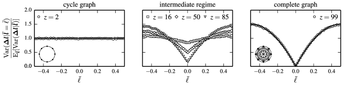
Figure 2: Normalized conditional variance ${\Var(\bm{\Delta l}|{\bm{\bar{l}}}=\bar{\ell})}/{\E_{{\bm{\bar{l}}}}[{\Var(\bm{\Delta l}|{\bm{\bar{l}}})}]}$ as a function of $\bar{\ell}$ for graphs with $N=100$ and varying $z$ values. For each value of $z$, data points correspond to ensemble averages (repeated simulations) with $4.95\text{\times}{10}^{6}$ springs in total. We use local linear regression with $3\text{\times}{10}^{4}$ nearest neighbors to estimate the variance for different values of $\bar{\ell}$. The solid lines correspond to the analytically derived expressions for cycle and complete graph (illustrated in the insets). In the intermediate regime of connectivity, the variance shows a continuous transition between the two extreme cases.

II.2.2 Complete graph

For the case of the complete graph ($z=N-1$), the derivation of the conditional variance is significantly more involved. In order to obtain manageable algebraic expressions, one needs to carefully choose the cycle basis (i.e., spanning tree). This choice of basis leads to a tractable expression for $(\mathbf{C}\mathbf{C}^{T})^{-1}$, which can then be applied to reformulate the problem in terms of conditionally independent winding number random variables.

Figure 3: (a) The complete graph ($z=N-1$) for $N=9$ vertices, here shown as undirected graph for clarity. (b) A spanning tree of a directed version of the complete graph in (a). The chosen spanning tree is based at the vertex at the center and, from there, reaches out to all $N-1$ other vertices. The edge orientations of the spanning tree edges (black) are chosen such that they have opposite orientation with respect to a connecting cycle (see, e.g., the cycle formed by the gray edge).

We choose a spanning tree as shown in Fig. 3. For the following derivation, we label the edges such that the first $N-1$ edges correspond to the edges of the spanning tree. The other $m=N(N-1)/2-(N-1)$ edges are the ones that are added to the spanning tree to construct the fundamental cycles (here: all triangles). We order the cycles in $\mathbf{C}$ according to these edges and decompose the cycle matrix into two parts:

$$\mathbf{C}=(\underbrace{\mathbf{A}}_{N-1}|\underbrace{\mathbf{I}}_{N(N-1)/2-(N-1)})\,,$$ (17)

where $\mathbf{I}$ is the identity matrix.

Our first result is that for spanning tree edges $\bm{l}^{*}_{\text{st}}\coloneqq\{l^{*}_{i}\}_{i=1}^{N-1}$ we have that

$$\bm{l}^{*}_{\text{st}}=N^{-1}(\mathbf{C}^{T}\mathbf{C})_{\text{st}}\cdot{\bm{\bar{l}}}=N^{-1}\begin{pmatrix}\mathbf{A}^{T}\mathbf{A}&\mathbf{A}^{T}\end{pmatrix}\cdot{\bm{\bar{l}}}\,,$$ (18)

where $(\mathbf{C}^{T}\mathbf{C})_{\text{st}}$ corresponds to the first $N-1$ rows of $\mathbf{C}^{T}\mathbf{C}$. The importance of this result is that the symmetries of the complete graph allow it to extend to all edges. Indeed, each vertex of the complete graph defines a spanning tree as shown in Fig. 3; therefore every edge can be seen as such a spanning tree edge. Independence of the solution of the choice of the cycle basis, and therefore spanning tree, implies that the following derivations hold for all edges in the graph.

Since, by Eqs. 2 and 17,

$$(\bm{l^{*}})_{\text{st}}=\left(\mathbf{A}^{T}(\mathbf{A}\mathbf{A}^{T}+\mathbf{I})^{-1}\mathbf{A}\quad\mathbf{A}^{T}(\mathbf{A}\mathbf{A}^{T}+\mathbf{I})^{-1}\right)\cdot{\bm{\bar{l}}}\,,$$

proving Eq. 18 is equivalent to showing that

$$\mathbf{A}^{T}(\mathbf{A}\mathbf{A}^{T}+\mathbf{I})^{-1}=N^{-1}\mathbf{A}^{T}$$

$$\Leftrightarrow\;\left[(N-1)\mathbf{I}-\mathbf{A}^{T}\mathbf{A}\right]\mathbf{A}^{T}=0\,.$$ (19)

We can construct $\mathbf{A}^{T}\mathbf{A}\in\mathbb{R}^{(N-1)\times(N-1)}$ explicitly: The $ij$th entry counts the number of cycles that are shared by the edges $i$ and $j$—with a contribution of $1$ if the edges have the same orientation with respect to the cycle, and $-1$ otherwise. As can be seen in Fig. 3, two spanning tree edges only share one cycle with opposite orientations, hence $(A^{T}A)_{ij}=-1$ for $i\neq j$. Each edge is itself part of $N-2$ cycles, so $(A^{T}A)_{ij}=N-2$ for $i=j$:

$$\mathbf{A}^{T}\mathbf{A}=\begin{cases}N-2,\quad&\text{when}\;i=j\\ -1,\quad&\text{when}\;i\neq j\end{cases}=(N-1)\mathbf{I}-\mathbf{J}\,,$$ (20)

where $\mathbf{J}\in\mathbb{R}^{(N-1)\times(N-1)}$ is the matrix with ones everywhere. Substitution into Eq. 19 yields:

$$\mathbf{J}\mathbf{A}^{T}=0\,.$$ (21)

Equation 21 holds true since each column of $\mathbf{A}^{T}$ contains two nonzero entries, $1$ and $-1$, due to all fundamental cycles (triangles) involving two spanning tree edges with opposite orientations (Fig. 3).

We have therefore shown that for the spanning tree edges of the complete graph, the following relation holds:

$$\bm{l^{*}_{\text{st}}}=N^{-1}(\mathbf{C}^{T}\mathbf{C})_{\text{st}}\cdot{\bm{\bar{l}}}=N^{-1}(\mathbf{C}^{T}\bm{g})_{\text{st}}\,,$$ (22)

where $(\mathbf{C}^{T}\bm{g})_{\text{st}}$ is the vector of the first $N-1$ entries of $\mathbf{C}^{T}\bm{g}$, and $\bm{g}=\mathbf{C}{\bm{\bar{l}}}$ is the vector of winding numbers (Eq. 1). Equation 22 allows us to change perspective to winding number random variables. For a particular edge in the spanning tree, we compute $l^{*}_{\text{st}}=\frac{1}{N}\sum_{j=1}^{N-2}g_{j}$, and therefore, $\Delta l_{\text{st}}=\frac{1}{N}\sum_{j=1}^{N-2}g_{j}-\bar{l}_{\text{st}}\,,$ since the edge is contained in exactly $N-2$ fundamental cycles, which we have assumed correspond to the first $N-2$ entries in the $\bm{g}$ vector, and edge and cycle orientations are aligned. For the conditional random variable $\Delta l_{\text{st}}|_{\bar{l}_{\text{st}}={\bar{\ell}}}$, it follows that:

$$\Delta l_{\text{st}}|_{\bar{l}_{\text{st}}={\bar{\ell}}}=\frac{1}{N}\sum\limits_{j=1}^{N-2}g_{j}|_{\bar{l}_{\text{st}}={\bar{\ell}}}-{\bar{\ell}}\,.$$ (23)

Observe that the $g_{j}|_{\bar{l}_{\text{st}}={\bar{\ell}}}$ are independent random variables since their only potential dependence, their common edge, is conditioned out. Each winding number $g_{j}|_{\bar{l}_{\text{st}}={\bar{\ell}}}$ corresponds to a fundamental cycle that is a triangle (Fig. 3), i.e., involves only three edges of which one is fixed. Therefore we cannot use conditional pairwise independence of edge lengths as in the case of the cycle graph to compute the variance. Instead, we derive the winding number distribution of a triangle explicitly.

The initial edge lengths are distributed as $\bar{l}_{j}\sim\mathcal{U}(-0.5,0.5)$, so the winding numbers can only attain three values $\{-1,0,1\}$. In particular, $g_{j}|_{\bar{l}_{\text{st}}={\bar{\ell}}}={\bar{\ell}}+\bar{l}_{j_{1}}+\bar{l}_{j_{2}}$, where we choose positive signs since the lengths are distributed symmetrically around zero. We compute the probability of $g_{j}|_{\bar{l}_{\text{st}}={\bar{\ell}}}$ attaining the value zero:

$$\begin{split}P(g_{j}|_{\bar{l}_{\text{st}}={\bar{\ell}}}=0)&=P(\bar{l}_{j_{2}}\in[-{\bar{\ell}}-0.5,-{\bar{\ell}}+0.5])\\ &=\int\limits_{-{\bar{\ell}}-0.5}^{-{\bar{\ell}}+0.5}\chi_{[-0.5,0.5]}(x)\,dx=1-|{\bar{\ell}}|\,,\end{split}$$ (24)

where $\chi_{[-0.5,0.5]}(\cdot)$ is the characteristic function on the interval $[-0.5,0.5]$. The remaining probability is assigned to either $g_{j}|_{\bar{l}_{\text{st}}={\bar{\ell}}}=1$ or $g_{j}|_{\bar{l}_{\text{st}}={\bar{\ell}}}=-1$ depending on whether the given ${\bar{\ell}}$ is positive or negative:

$$P(g_{j}|_{\bar{l}_{\text{st}}={\bar{\ell}}\geq 0}=1)=P(g_{j}|_{\bar{l}_{\text{st}}={\bar{\ell}}\leq 0}=-1)=|{\bar{\ell}}|\,.$$ (25)

Using Eq. 23, conditional independence of the $g_{j}|_{\bar{l}_{\text{st}}={\bar{\ell}}}$, and their probability distribution, Eqs. 24 and 25, we have:

$$\Var(\Delta l_{\text{st}}|{\bar{l}_{\text{st}}={\bar{\ell}}}) =\frac{N-2}{N^{2}}\Var(g_{j}|\bar{l}_{\text{st}}={\bar{\ell}})$$ (26)

$$=\frac{N-2}{N^{2}}(|{\bar{\ell}}|-{\bar{\ell}}^{2})\,.$$ (27)

In contrast to the cycle graph (Eq. 16), the conditional variance ${\Var(\bm{\Delta l}|{\bm{\bar{l}}}=\bar{\ell})}=\Var(\Delta l_{\text{st}}|{\bar{l}_{\text{st}}={\bar{\ell}}})$ for the complete graph (Eq. 27) depends on the initial spring length $\bar{\ell}$, as is shown in Fig. 2.

II.2.3 Intermediate-connectivity regime

For the intermediate-connectivity regime, $2<z<N-1$, a tractable expression for $(\mathbf{C}\mathbf{C}^{T})^{-1}$, as for the complete graph, remains elusive; however, numerical data suggest that the variance exhibits a continuous transition between the two extremes (Fig. 2). We also observe that the conditional variance is approximately constant given that $z\ll N$. This is the most relevant case for biological networks where typically $z\lesssim 4$. For $z\ll N$, we may thus approximate ${\Var(\bm{\Delta l}|{\bm{\bar{l}}}=\bar{\ell})}\approx{\E_{{\bm{\bar{l}}}}[{\Var(\bm{\Delta l}|{\bm{\bar{l}}})}]}$, which we now derive.

The law of total variance Weiss (2006) states:

$$\E_{{\bm{\bar{l}}}}[\Var(\bm{\Delta l}\,|\,{\bm{\bar{l}}})]=\Var(\bm{\Delta l})-\Var_{{\bm{\bar{l}}}}[\E(\bm{\Delta l}\,|\,{\bm{\bar{l}}})]\,.$$ (28)

We first compute $\Var(\bm{\Delta l})$, again, by initially fixing $\mathbf{S}$ and considering $\Var(\bm{\Delta l}|\mathbf{S})$. With Eqs. 10 and 9 we compute

$$\Var[\bm{\Delta l}|\mathbf{S}]=\frac{2}{Nz}\sum_{i=1}^{Nz/2}\Var(\Delta l_{i}|\mathbf{S})=\frac{2\Var(\bar{l})}{Nz}\sum_{i,j=1}^{Nz/2}S_{ij}^{2}\,,$$

where the second equality follows from fixed-graph ensembles having uniformly distributed edge random variables that are pairwise independent. Again, we use that $\mathbf{P}^{2}=\mathbf{P}$, hence $\mathbf{S}^{2}=-\mathbf{S}$, and therefore $\sum_{j=1}^{Nz/2}S_{ij}^{2}=-S_{ii}$. Insertion into the equation above yields:

$$\frac{\Var(\bm{\Delta l}|\mathbf{S})}{\Var(\bar{l})}=-\frac{2\tr\mathbf{S}}{Nz}=\frac{2}{z}\left(1-\frac{1}{N}\right)\,,$$ (29)

where the second equality is due to Eq. 12. Application of the law of total variance gives:

$$\begin{split}\Var(\bm{\Delta l})&=\E_{\mathbf{S}}[\Var(\bm{\Delta l}|\mathbf{S})]+\Var_{\mathbf{S}}[\underbrace{\E(\bm{\Delta l}|\mathbf{S})}_{=0}]\\ &=\frac{2}{z}\left(1-\frac{1}{N}\right)\Var(\bar{l})\,,\end{split}$$ (30)

where the second term in the sum vanishes using Eq. 10 since $\E(\bar{l}_{i})=0$ (analogous to the computation in Eq. 11). From Eq. 13 we can use $\Var_{{\bm{\bar{l}}}}[\E(\bm{\Delta l}\,|\,{\bm{\bar{l}}})]={(2/z(1-1/N))^{2}\Var(\bar{l})}$ and therefore find by substituting into Eq. 28:

$$\frac{\E_{{\bm{\bar{l}}}}[{\Var(\bm{\Delta l}|{\bm{\bar{l}}})}]}{{\Var(\bar{l})}} =\frac{2}{z}\left(1-\frac{1}{N}\right)\left[1-\frac{2}{z}\left(1-\frac{1}{N}\right)\right]\,.$$ (31)

II.3 Normality

If $\bm{\Delta l}|_{{\bm{\bar{l}}}={\bar{\ell}}}$ were normally distributed, having estimates for mean and variance (Eqs. 13 and 31) would be sufficient to fully characterize $p_{{\bm{\Delta l}|{\bm{\bar{l}}}=\bar{\ell}}}$. Indeed, for the two extremes, cycle and complete graph, we can prove that $\bm{\Delta l}|_{{\bm{\bar{l}}}={\bar{\ell}}}$ is normally distributed in the limit $N\to\infty$, with a rate of convergence proportional to $(N-2)^{-1/2}$.

This result might look like a direct application of the classical central limit theorem. However, since the edge lengths are not independent as random variables, more sophisticated techniques are required to represent the solution in terms of a suitable set of mutually independent random variables. In contrast to situations in time series analysis Brockwell and Davis (2009), where independence holds beyond a certain time window, in our case the cycle constraints prohibit localization of dependencies. To deal with this problem, we reduce the number of variables by relaxing each integer cycle constraint to an interval constraint. Harnessing the resulting independence then requires a non-standard transformation of random variables, which complicates a direct application of the Berry-Esseen theorem Berry (1941); Esseen (1942) (a deviation-bound version of the central-limit theorem) to obtain a quantitative bound on the distance to a normal distribution.

The rest of this section is split into three parts. We begin by proving the results for the cycle and complete graph, and then investigate the intermediate-connectivity regime. Throughout, note how the intricacies of the proofs of the extreme cases are further complicated in the intermediate-connectivity regime, where ensembles have varying graph structure and lack symmetry.

II.3.1 Cycle graph

For the cycle graph ($z=2$), we prove that $\Delta l_{i}|_{\bar{l}_{i}={\bar{\ell}}}$ is normally distributed in the limit $N\to\infty$. The key idea is a relaxation of the integer constraint to an interval constraint. Using $\Delta l_{i}=g/N-\bar{l}_{i}=\sum_{j=1}^{N}\bar{l}_{j}/N-\bar{l}_{i}$ (Eq. 14) we introduce the standardized ($\E(Y_{N})=0$, $\Var(Y_{N})=1$) random variable

$$Y_{N} \coloneqq\frac{\Delta l_{i}|_{\bar{l}_{i}={\bar{\ell}}}-\E(\Delta l_{i}|\bar{l}_{i}={\bar{\ell}})}{\sqrt{\Var(\Delta l_{i}|\bar{l}_{i}={\bar{\ell}})}}$$ (32)

$$=\frac{g|_{\bar{l}_{i}={\bar{\ell}}}/N-{\bar{\ell}}-({\bar{\ell}}/N-{\bar{\ell}})}{\sqrt{\frac{N-1}{N^{2}}{\Var(\bar{l})}}}$$ (33)

$$=\frac{g|_{\bar{l}_{i}={\bar{\ell}}}-{\bar{\ell}}}{\sqrt{(N-1){\Var(\bar{l})}}}\,,$$ (34)

and compare its cdf $F_{Y_{N}}(x)$ to that of the standard normal $\Phi_{0,1}(x)$. We find that

$$F_{Y_{N}}(x) =\Prob(Y_{N}\leq x)$$ (35)

$$=\Prob\left(g|_{\bar{l}_{i}={\bar{\ell}}}\leq x\,\sqrt{(N-1){\Var(\bar{l})}}+{\bar{\ell}}\right)$$ (36)

$$=\sum_{k=-\infty}^{\left\lfloor x\,\sqrt{(N-1){\Var(\bar{l})}}+{\bar{\ell}}\right\rfloor}\Prob(g|_{\bar{l}_{i}={\bar{\ell}}}=k)\,,$$ (37)

where we have used the fact that $g\in\mathbb{Z}$ and $\lfloor\cdot\rfloor$ denotes the floor operator. Using $g|_{l_{i}={\bar{\ell}}}={\bar{\ell}}+\sum_{j=1,\,j\neq i}^{N}\bar{l}_{j}$ we can formalize the integer relaxation by expressing the probability of the conditional winding number as follows:

$$\Prob(g|_{\bar{l}_{i}={\bar{\ell}}}=k)=\int_{k-{\bar{\ell}}-0.5}^{k-{\bar{\ell}}+0.5}\nu_{N-2}(t)\,dt\,,$$ (38)

where $\nu_{N-2}(t)$ corresponds to the probability density of the sum of $N-2$ uniformly distributed independent random variables on the interval $[-0.5,0.5]$. We call this random variable $U_{N-2}$. There are only $N-2$ independent random variables because one of the $N$ lengths is fixed to ${\bar{\ell}}$ and another one is determined to make sure that an integer winding number is attained for $g$. Substituting Eq. 38 into Eq. 37 and expressing $\left\lfloor x\,\sqrt{(N-1){\Var(\bar{l})}}+{\bar{\ell}}\right\rfloor=x\,\sqrt{(N-1){\Var(\bar{l})}}+{\bar{\ell}}-\delta(x)$, with the random variable $\delta(x)\in[0,1)$, leads to:

$$F_{Y_{N}}(x) =\sum_{k=-\infty}^{x\,\sqrt{(N-1){\Var(\bar{l})}}+{\bar{\ell}}-\delta(x)}\int_{k-{\bar{\ell}}-0.5}^{k-{\bar{\ell}}+0.5}\nu_{N-2}(t)\,dt$$

$$=\int_{-\infty}^{x\,\sqrt{(N-1){\Var(\bar{l})}}+0.5-\delta(x)}\nu_{N-2}(t)\,dt$$

$$=F_{U_{N-2}}\left(x\,\sqrt{(N-1){\Var(\bar{l})}}+0.5-\delta(x)\right)\,.$$

We are interested in the distance to the cdf $\Phi_{0,1}(x)$ of the standard normal distribution. To calculate this distance, this we perform a change of variables which results in a standardized sum of uniforms $U_{N-2}/(\sigma_{\bar{l}}\sqrt{N-2})$, where $\sigma_{\bar{l}}=\sqrt{\Var{(\bar{l})}}$. However, this causes the cdf of our random variable and the standard normal cdf to have different arguments. We therefore split the computation into two steps: one that measures the distance to a shifted standard normal cdf, and the other that measures the deviations introduced by this shift. With the shorthand notation $\xi(x)\coloneqq x\,\sqrt{(N-1){\Var(\bar{l})}}+0.5-\delta(x)$, the described procedure corresponds to the following computation:

$$|F_{Y_{N}}(x)-\Phi_{0,1}(x)|=\left|F_{U_{N-2}}\left(\xi(x)\right)-\Phi_{0,1}(x)\right|$$

$$=\left|F_{\frac{U_{N-2}}{\sigma_{\bar{l}}\sqrt{N-2}}}\left(\frac{\xi(x)}{\sigma_{\bar{l}}\sqrt{N-2}}\right)-\Phi_{0,1}(x)\right|$$

$$\leq\underbrace{\left|F_{\frac{U_{N-2}}{\sigma_{\bar{l}}\sqrt{N-2}}}\left(\frac{\xi(x)}{\sigma_{\bar{l}}\sqrt{N-2}}\right)-\Phi_{0,1}\left(\frac{\xi(x)}{\sigma_{\bar{l}}\sqrt{N-2}}\right)\right|}_{\eqqcolon I(x)}$$

$$+\underbrace{\left|\Phi_{0,1}\left(\frac{\xi(x)}{\sigma_{\bar{l}}\sqrt{N-2}}\right)-\Phi_{0,1}(x)\right|}_{\eqqcolon II(x)}\,.$$

$I(x)$ can be bounded using the Berry-Esseen theorem. Bounding $II(x)$ requires a detailed case analysis (see Appendix B for details). We arrive at:

$$\sup_{x\in\mathbb{R}}|F_{Y_{N}}(x)-\Phi_{0,1}(x)|\leq I(x)+II(x)$$ (39)

$$\leq\frac{12^{3/2}\,C}{32\sqrt{N-2}}+\frac{1}{\sqrt{2\pi(N-2){\Var(\bar{l})}}}$$ (40)

$$=\frac{1}{\sqrt{N-2}}\left(\frac{12^{3/2}\,C}{32}+\frac{1}{\sqrt{2\pi{\Var(\bar{l})}}}\right)\,.$$ (41)

Therefore, the cdf of $\Delta l_{i}|_{\bar{l}_{i}={\bar{\ell}}}$ converges to a normal distribution with the rate $(N-2)^{-1/2}$, independent of ${\bar{\ell}}$. Since we showed that $F_{\Delta l_{i}|\bar{l}_{i}={\bar{\ell}}}$ is independent of the edge $i$, Eq. 4 implies $F_{{\bm{\Delta l}|{\bm{\bar{l}}}=\bar{\ell}}}\,(x)=F_{\Delta l_{i}|\bar{l}_{i}={\bar{\ell}}}\,(x)$, and therefore $F_{{\bm{\Delta l}|{\bm{\bar{l}}}=\bar{\ell}}}$ converges to a normal distribution as well.

II.3.2 Complete graph

For the complete graph, our proof of normality relies on the reduction to spanning tree edges as outlined in the conditional variance section. In particular, this allows us to write the cdf in terms of winding number random variables that are all triangles that share a common edge. Conditioning on this edge then yields independence, not of the length variables, but of these winding number random variables, which allows us to apply the Berry-Esseen theorem.

To measure how far $\Delta l_{\text{st}}|_{\bar{l}_{\text{st}}={\bar{\ell}}}$ is from being normally distributed for finite $N$, we look at the standardized random variable

$$Y_{N-2}\coloneqq\frac{\Delta l_{\text{st}}|_{\bar{l}_{\text{st}}={\bar{\ell}}}-\E(\Delta l_{\text{st}}|{\bar{l}_{\text{st}}={\bar{\ell}}})}{\sqrt{\Var(\Delta l_{\text{st}}|{\bar{l}_{\text{st}}={\bar{\ell}}})}}$$ (42)

and compare its cdf to the one of the standard normal. Using Eq. 23 and the probability distribution of $g_{j}|_{\bar{l}_{\text{st}}={\bar{\ell}}}$, Eqs. 24 and 25, we obtain:

$$\E(\Delta l_{\text{st}}|\bar{l}_{\text{st}}={\bar{\ell}}) =\frac{N-2}{N}\E(g_{j}|\bar{l}_{\text{st}}={\bar{\ell}})-{\bar{\ell}}$$ (43)

$$=\frac{(N-2){\bar{\ell}}}{N}-{\bar{\ell}}\,,$$ (44)

$$\Var(\Delta l_{\text{st}}|{\bar{l}_{\text{st}}={\bar{\ell}}}) =\frac{N-2}{N^{2}}\Var(g_{j}|\bar{l}_{\text{st}}={\bar{\ell}})$$ (45)

$$=\frac{N-2}{N^{2}}(|{\bar{\ell}}|-{\bar{\ell}}^{2})\,,$$ (46)

and therefore

$$Y_{N-2} =\frac{\frac{1}{N}\sum_{j=1}^{N-2}g_{j}|_{\bar{l}_{\text{st}}={\bar{\ell}}}-\frac{(N-2){\bar{\ell}}}{N}}{\sqrt{\frac{N-2}{N^{2}}\Var(g_{j}|\bar{l}_{\text{st}}={\bar{\ell}})}}$$ (47)

$$=\frac{\sum_{j=1}^{N-2}(g_{j}|_{\bar{l}_{\text{st}}={\bar{\ell}}}-{\bar{\ell}})}{\sqrt{\sum_{j=1}^{N-2}\Var(g_{j}|_{\bar{l}_{\text{st}}={\bar{\ell}}}-{\bar{\ell}})}}\,.$$ (48)

All $\{g_{j}|_{\bar{l}_{\text{st}}={\bar{\ell}}}\}_{j=1}^{N-2}$ are independent since the corresponding cycles only share one edge, which is the one that we condition on. We can thus apply the Berry-Esseen theorem (Theorem) to show that for $N\geq 3$,

$$\sup_{x\in\mathbb{R}}|F_{Y_{N-2}}(x)-\Phi_{0,1}(x)|\leq\frac{C\rho}{\sigma^{3}\sqrt{N-2}}\,,$$ (49)

with $C<0.4748$, $\rho=\E(\left|g_{j}|_{\bar{l}_{\text{st}}={\bar{\ell}}}-{\bar{\ell}}\right|^{3})$, and $\sigma^{2}=\Var(g_{j}|_{\bar{l}_{\text{st}}={\bar{\ell}}}-{\bar{\ell}})=|{\bar{\ell}}|-{\bar{\ell}}^{2}$. Computing $\rho=(|{\bar{\ell}}|-{\bar{\ell}}^{2})({\bar{\ell}}^{2}+(1-|{\bar{\ell}}|)^{2})$ via Eqs. 24 and 25 we arrive at

$$\sup_{x\in\mathbb{R}}|F_{Y_{N-2}}(x)-\Phi_{0,1}(x)|\leq\frac{C}{\sqrt{N-2}}\frac{{\bar{\ell}}^{2}+(1-|{\bar{\ell}}|)^{2}}{\sqrt{|{\bar{\ell}}|-{\bar{\ell}}^{2}}}\,,$$ (50)

for $|{\bar{\ell}}|>0$. This proves convergence of the cdf of $\Delta l_{i}|_{\bar{l}_{i}={\bar{\ell}}}$ to a normal distribution with the rate $(N-2)^{-1/2}$. For ${\bar{\ell}}=0$, $\Delta l_{i}|_{\bar{l}_{i}={\bar{\ell}}}\sim\delta_{0}$ (Dirac delta distribution around zero), it can only attain the value zero because $P(g_{j}|_{\bar{l}_{\text{st}}={\bar{\ell}}}=0)=1$.

Note the ${\bar{\ell}}$-dependence in Eq. 50, which is in stark contrast to the ${\bar{\ell}}$-independent bound for the cycle graph (Eq. 41). For the complete graph, the approximation with a normal distribution becomes worse as ${\bar{\ell}}$ approaches zero.

II.3.3 Intermediate-connectivity regime

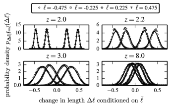
Figure 4: Conditional probability density $p_{{\bm{\Delta l}|{\bm{\bar{l}}}=\bar{\ell}}}\,(\Delta\ell)$ for spring networks with $N=100$ and varying $z$, conditioned on different $\bar{\ell}$ values. For each value of $z$, data points correspond to ensemble averages (repeated simulations) with $4.95\text{\times}{10}^{6}$ springs in total. Solid lines correspond to best-fit normal distributions. The cycle graph ($z=2$) is close to being normally distributed—as proven for $N\to\infty$. Whereas for $z=2.2$, there are still deviations from a normal distribution, for $z=3$ and larger, the densities rapidly approach a normal distribution.

Recall that in the intermediate-connectivity regime, $2<z<N-1$, the $(N,z)$-ensembles contain graphs with varying cycle structures making a similar analysis significantly more challenging. In simulations, however, we observe that $\bm{\Delta l}|_{{\bm{\bar{l}}}={\bar{\ell}}}$ is approximately normally distributed if $z$ is sufficiently large (Fig. 4).

II.4 Density approximation

Our empirical observations and theoretical discussion above justify the following approximation for $3\leq z\ll N$:

$$\bm{\Delta l}|_{{\bm{\bar{l}}}={\bar{\ell}}}\sim\mathcal{N}\Big{[}\E({\bm{\Delta l}|{\bm{\bar{l}}}=\bar{\ell}}),E_{{\bm{\bar{l}}}}[{\Var(\bm{\Delta l}|{\bm{\bar{l}}})}]\Big{]}\,,$$ (51)

with the expressions for $\E({\bm{\Delta l}|{\bm{\bar{l}}}=\bar{\ell}})$ and $E_{{\bm{\bar{l}}}}[{\Var(\bm{\Delta l}|{\bm{\bar{l}}})}]$ given in Eqs. 13 and 31. Using Eqs. 7 and 51, we obtain an explicit representation for the final length distribution $p_{\bm{l^{*}}}({\ell^{*}})$ in mechanical equilibrium (Appendix C). In Fig. 5 we compare this analytical expression to ensembles of simulated networks and observe excellent agreement.

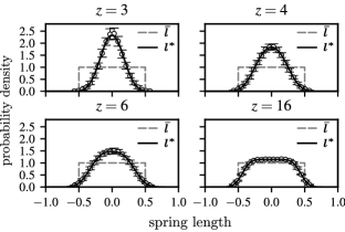
Figure 5: Probability density $p_{\bm{l^{*}}}(\ell^{*})$ for the final spring lengths for networks with $N=1000$ and varying $z$. Solid black lines show the analytic expression for $p_{\bm{l^{*}}}(\ell^{*})$ (Eq. 78); data points correspond to averages over 50 simulations. The error bars correspond to the standard deviation. For comparison, we show the initial uniform spring length distribution $p_{{\bm{\bar{l}}}}({\bar{\ell}})$ as a gray dashed line.

III Comparison to a mean-field approach

In order to evaluate the significance of our graph-theoretical analysis we compare it to a mean-field (mf) approach which neglects all topological features other than the local degree of connectivity.

Figure 6: Mean-field approach (here: $z=4$): The edge $\bar{l}$ connects two nodes $(\mathrm{n_{1}},\mathrm{n_{2}})$. The initial node forces (gray arrows) are given by $f_{\mathrm{n}_{1}}=\sum_{i=1}^{z-1}\bar{l}_{\mathrm{n}_{1},i}+\bar{l}$ and $f_{\mathrm{n}_{2}}=\sum_{i=1}^{z-1}\bar{l}_{\mathrm{n}_{2},i}-\bar{l}$. The spring $\bar{l}$ contributes to the forces with different signs because its length is measured from $\mathrm{n_{1}}$ to $\mathrm{n_{2}}$ (depicted by the black triangle). While displacing an individual node by $u_{\mathrm{n_{k}}}=z^{-1}f_{\mathrm{n_{k}}}$ introduces force balance at that node, this approach neglects that nodes/edges are coupled, i.e., force balance has to be established at all nodes simultaneously, as in Eq. 1.

In contrast to the graph-theoretical model, where $z$ refers to the average degree of a node, the mean-field approach assumes that each node is connected to exactly $z$ other nodes. Moreover, the node displacement $u_{\text{node}}$ during relaxation is calculated as if all other nodes in the network were fixed. Therefore $u_{\text{node}}=f_{\text{node}}/z$, where $f_{\text{node}}=\sum_{i=1}^{z}\bar{l}_{i}$ is the initial force acting on the node via the springs attached to it. The displacement $\Delta l$ of a spring is given by the difference of the displacements of the two nodes that are connected by this edge:

$$\begin{split}\Delta l&=u_{\mathrm{n}_{2}}-u_{\mathrm{n}_{1}}=z^{-1}(f_{\mathrm{n}_{2}}-f_{\mathrm{n}_{1}})\\ &=\frac{1}{z}\left(-2\bar{l}+\sum_{i=1}^{z-1}\bar{l}_{\mathrm{n}_{2},i}-\sum_{i=1}^{z-1}\bar{l}_{\mathrm{n}_{1},i}\right)\,,\end{split}$$ (52)

where we have taken into account that the two nodes share one spring, namely $\bar{l}$ (Fig. 6). All springs are assumed to be independent identically distributed random variables with mean zero and variance ${\Var(\bar{l})}$.

For the conditional mean, we have with Eq. 52:

$$\E({\bm{\Delta l}|{\bm{\bar{l}}}=\bar{\ell}})|_{\text{mf}}=-\frac{2{\bar{\ell}}}{z}\,.$$ (53)

The mean-field result agrees with the exact solution Eq. 13 in the limit $N\to\infty$, i.e., there is no significant difference for large node numbers. In contrast, we will show at the end of this section that for the variance, the mean-field solution differs substantially from the exact result, even in the limit $N\to\infty$.

When considering normality of $\bm{\Delta l}|_{{\bm{\bar{l}}}={\bar{\ell}}}$, the mean-field approach allows us to directly apply the Berry-Esseen theorem (Theorem) because all edges are treated as independent. Defining the normalized random variable

$$Y_{2(z-1)}:= \frac{\Delta l|_{\bar{l}={\bar{\ell}}}-\E(\Delta l|{\bar{l}}={\bar{\ell}})}{\sqrt{\Var(\Delta l|{\bar{l}={\bar{\ell}}})}}$$ (54)

$$= \frac{\sum_{i=1}^{2(z-1)}\bar{l}_{i}}{\sqrt{2(z-1)\Var(\bar{l})}}\,,$$ (55)

the theorem implies:

$$\sup_{x\in\mathbb{R}}|F_{Y_{2(z-1)}}(x)-\Phi_{0,1}(x)|\leq\frac{12^{3/2}\,C}{32\sqrt{2(z-1)}}\,.$$ (56)

The mean-field approach yields convergence to a normal distribution with a rate proportional to $(z-1)^{-1/2}$. While this result agrees with the rate of convergence we proved for the complete graph, it is in stark contrast to what we proved for the cycle graph case ($z=2$), for which we showed convergence to a normal distribution even though $z$ is constant. In the intermediate-connectivity regime, both the mean-field as well as our graph-theoretical approach suggest that $\bm{\Delta l}|_{{\bm{\bar{l}}}={\bar{\ell}}}$ can be approximated by a normal distribution. To complete the evaluation of our approach, it is therefore critical to also compare the second moments, i.e., the variances of the mean-field and graph-theoretical approach.

For the unconditional variance, we obtain using Eq. 52:

$$\Var(\bm{\Delta l})|_{\text{mf}} =z^{-2}\left(4{\Var(\bar{l})}+2(z-1){\Var(\bar{l})}\right)$$ (57)

$$=\frac{2}{z}\left(1+\frac{1}{z}\right){\Var(\bar{l})}\,.$$ (58)

Clearly, this expression does not agree with the exact graph-theoretical value Eq. 30, even in the limit $N\to\infty$. A mean-field approach assumes the conditional variance is constant and therefore equal to its expected value $\E_{{\bm{\bar{l}}}}[{\Var(\bm{\Delta l}|{\bm{\bar{l}}})}]|_{\text{mf}}={\Var(\bm{\Delta l}|{\bm{\bar{l}}}=\bar{\ell})}|_{\text{mf}}={2/z(1-1/z)\Var(\bar{l})}$. For the cycle graph, we proved the conditional variance is indeed constant (Eq. 16). However, we showed that the other extreme, the complete graph, exhibits non-constant conditional variance (Eq. 27). For $(N,z)$-ensembles in the intermediate-connectivity regime, we observe a continuous transition between the two extremes (Fig. 7). Therefore, for the biological regime ($z\lesssim 4$), we approximated the conditional variance with its constant expected value $\E_{{\bm{\bar{l}}}}[{\Var(\bm{\Delta l}|{\bm{\bar{l}}})}]$ (Eq. 31). However, it is exactly the regime $z\lesssim 4$ where the graph-theoretically derived expected conditional variance $\E_{{\bm{\bar{l}}}}[{\Var(\bm{\Delta l}|{\bm{\bar{l}}})}]$ and the mean-field quantity $\E_{{\bm{\bar{l}}}}[{\Var(\bm{\Delta l}|{\bm{\bar{l}}})}]|_{\text{mf}}$ exhibit the largest discrepancy (Fig. 7).

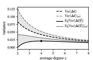
Figure 7: Comparison of graph-theoretical (black) and mean-field (gray) variances as a function of average degree $z$. Shown are the unconditional variance ${\Var(\bm{\Delta l})}$ as well as the expected conditional variance ${\E_{{\bm{\bar{l}}}}[{\Var(\bm{\Delta l}|{\bm{\bar{l}}})}]}$ as derived in the text. The graph-theoretically derived expected variance exhibits a maximum at $z=4$ (filled circle), while the corresponding mean-field expected variance monotonically decreases from its value at $z=2$.

IV Discussion and conclusions

In conclusion, we have presented a probabilistic theory of force distributions in one-dimensional random spring networks on a circle. Here we have regarded networks with initially unbalanced forces that relax into mechanical equilibrium. When drawing the analogy to a biological network, our approach, which focuses on the relaxation of the system after non-equilibrium starting conditions, is equivalent to assuming a separation of time scales where internal or external non-equilibrium processes slowly create forces in the network that rapidly equilibrate.

We developed a graph-theoretical approach that allows us to exactly compute mean and expected variance of the distribution of length changes conditioned on an initial configuration. For the two extreme cases, the cycle graph and the complete graph, we could prove convergence of this distribution to a normal distribution. A systematic analytical treatment of the—less symmetric—intermediate-connectivity regime is more demanding and not provided here. However, our results suggest an approximation that shows excellent agreement with simulation for the biologically relevant regime of connectivity, $3\leq z\ll N$.

It is straightforward to generalize the approach we present here to higher spatial dimensions $d$ if the probability densities $p_{{\bm{\bar{l}}}_{k}}$ for the components of the initial spring vectors are independent. In that case, due to the linearity of spring forces with extension, the optimization problem decouples into the spatial components. The probability density for the final spring vectors then is simply given as the product of the one-dimensional results:

$$p_{\bm{l^{*}}}(\bm{\ell^{*}})=\prod\limits_{k=1}^{d}p_{\bm{l^{*}}_{k}}(\ell^{*}_{k})\,.$$ (59)

Hence, our results carry over to two- and three-dimensional networks, which are more commonly studied in practice and are of biological and physiological relevance.

Interestingly, a classical mean-field approach fails to correctly reproduce the mean and the variance of the relevant distributions. The error is particularly pronounced for the—biologically most relevant—regime of low degrees of connectivity, and does not vanish in the limit of infinite node number. Our work demonstrates that network topology—here manifested as cycle constraints—is crucial for the correct determination of force distributions in an elastic spring network.

This opens the door for future research on the role of network topology in more complex elastic networks, e.g., in the presence of dynamics, spring nonlinearities or rupture. Moreover, the mixture of probabilistic and graph-theoretical techniques may prove useful for other types of network theories.

Appendix A Independence of the choice of cycle basis

A change of cycle basis corresponds to the transformation

$$\mathbf{\tilde{C}}=\mathbf{Q}\mathbf{C}\mathbf{\mathbf{U}}^{-1}\,,$$ (60)

where $\mathbf{Q}\in\mathrm{GL}(m)$ is an arbitrary change of basis matrix for the cycle space, and $\mathbf{U}\in\mathrm{O}(Nz/2)$ is a permutation matrix that corresponds to relabeling the edges of the graph. The independence of the solution of the cycle matrix means that, given the change of basis in Eq. 60 and the solution (Eq. 2)

$$\bm{\tilde{l}^{*}}=\mathbf{\tilde{C}}^{T}(\mathbf{\tilde{C}}\mathbf{\tilde{C}}^{T})^{-1}\mathbf{\tilde{C}}\bm{\tilde{\bar{l}}}$$

to the transformed problem,

$$\bm{\tilde{l}^{*}}=\mathbf{U}\,\bm{l^{*}}\,.$$ (61)

The above relation can be shown by direct computation:

$$\mathbf{\tilde{C}}^{T}(\mathbf{\tilde{C}}\mathbf{\tilde{C}}^{T})^{-1}\mathbf{\tilde{C}} =(\mathbf{Q}\mathbf{C}\mathbf{U}^{-1})^{T}(\mathbf{Q}\mathbf{C}\mathbf{U}^{-1}(\mathbf{Q}\mathbf{C}\mathbf{U}^{-1})^{T})^{-1}(\mathbf{Q}\mathbf{C}\mathbf{U}^{-1})=\mathbf{U}^{-T}\mathbf{C}^{T}\mathbf{Q}^{T}(\mathbf{Q}\mathbf{C}\mathbf{U}^{-1}\mathbf{U}^{-T}\mathbf{C}^{T}\mathbf{Q}^{T})^{-1}(\mathbf{Q}\mathbf{C}\mathbf{U}^{-1})$$

$$=\mathbf{U}^{-T}\mathbf{C}^{T}\mathbf{Q}^{T}\mathbf{Q}^{-T}(\mathbf{C}\mathbf{C}^{T})^{-1}\mathbf{Q}^{-1}\mathbf{Q}\mathbf{C}\mathbf{U}^{-1}=\mathbf{U}\mathbf{C}^{T}(\mathbf{C}\mathbf{C}^{T})^{-1}\mathbf{C}\mathbf{U}^{-1}\,,$$

and therefore

$$\bm{\tilde{l}^{*}} =\mathbf{U}\mathbf{C}^{T}(\mathbf{C}\mathbf{C}^{T})^{-1}\mathbf{C}\mathbf{U}^{-1}\bm{\tilde{\bar{l}}}=\mathbf{U}\mathbf{C}^{T}(\mathbf{C}\mathbf{C}^{T})^{-1}\mathbf{C}{\bm{\bar{l}}}=\mathbf{U}\bm{l^{*}}\,.$$

Appendix B Upper bounds for $\mathbf{I(x)}$ and $\mathbf{II(x)}$

For a uniform upper bound on the first term $I(x)$, we can apply the Berry-Esseen theorem, which is stated as follows Athreya and Lahiri (2006).

Theorem (Berry-Esseen).

Let $X_{1},X_{2},\cdots$ be independent identically distributed (iid) random variables with $E(X_{1})=0$, $E(X_{1}^{2})=\sigma^{2}>0$, $E(|X_{1}|^{3})=\rho<\infty$. Also, let

$$S_{n}=\frac{X_{1}+X_{2}+\cdots+X_{n}}{\sqrt{n}\sigma}$$

be the normalized $n$-th partial sum. Denote $F_{n}$ the cdf of $S_{n}$, and $\Phi_{0,1}$ the cdf of the standard normal distribution. Then there exists a positive constant $C<0.4785$ Tyurin (2010) such that

$$\sup_{x\in\mathbb{R}}|F_{n}(x)-\Phi_{0,1}(x)|\leq\frac{C\rho}{\sigma^{3}\sqrt{n}}\,.$$ (62)

By recalling that $U_{N-2}$ is the sum of $N-2$ independent uniformly distributed random variables on the interval $[-1/2,1/2]$, i.e., with variance ${\Var(\bar{l})}=\sigma^{2}_{\bar{l}}=1/12$, third absolute moment $\rho_{\bar{l}}=1/32$, and mean $\E(\bar{l})=0$, we have that $U_{N-2}/(\sigma_{\bar{l}}\sqrt{N-2})$ is a normalized $n$-th partial sum. The Berry-Esseen theorem therefore implies:

$$\sup_{x\in\mathbb{R}}I(x)=\sup_{x\in\mathbb{R}}\left|F_{\frac{U_{N-2}}{\sigma_{\bar{l}}\sqrt{(N-2)}}}(x)-\Phi_{0,1}(x)\right|\leq\frac{12^{3/2}\,C}{32\sqrt{N-2}}\,.$$ (63)

An upper bound for the second term $II(x)$ can be found as well. We write:

$$II(x) =\left|\Phi_{0,1}\left(\frac{x\,\sqrt{(N-1){\Var(\bar{l})}}+0.5-\delta(x)}{\sqrt{(N-2){\Var(\bar{l})}}}\right)-\Phi_{0,1}(x)\right|$$ (64)

$$=\left|\Phi_{0,1}(\alpha x+\beta)-\Phi_{0,1}(x)\right|=\left|\Phi_{0,1}(y)-\Phi_{0,1}(x)\right|\,,$$ (65)

with $\alpha=\sqrt{\frac{N-1}{N-2}}$, $\beta=\frac{0.5-\delta(x)}{\sqrt{(N-2){\Var(\bar{l})}}}$, and $y=\alpha x+\beta$. There are six cases that need to be distinguished: $(x<0<y)$, $(y<0<x)$, $(x<y<0)$, $(y<x<0)$, $(0<x<y)$, $(0<y<x)$.

For $(y<0<x)$, the following holds:

$$\left|\Phi_{0,1}(\alpha x+\beta)-\Phi_{0,1}(x)\right| \leq[({1-\alpha})x-\beta]\,\sup_{x\in\mathbb{R}}\Phi^{\prime}_{0,1}(x)\leq-\frac{\beta}{\sqrt{2\pi}}$$ (66)

$$<\frac{1}{2\sqrt{2\pi(N-2){\Var(\bar{l})}}}\,,$$ (67)

where we have used that $1-\alpha<0$ and $\delta(x)\in[0,1)$. Analogously, the same bound holds for the case $(x<0<y)$. For the other cases, we can make use of the convexity (concavity) of $\Phi_{0,1}(x)$ for $x<0$ ($x>0$).

For $(x<y<0)$, we have:

$$\left|\Phi_{0,1}(\alpha x+\beta)-\Phi_{0,1}(x)\right| \leq[({\alpha-1})x+\beta]\,\Phi^{\prime}_{0,1}(\alpha x+\beta)$$ (68)

$$=[(\alpha-1)x+\beta](2\pi)^{-1/2}e^{-(\alpha x+\beta)^{2}/2}$$ (69)

$$\leq\frac{\beta}{\sqrt{2\pi}}<\frac{1}{2\sqrt{2\pi(N-2){\Var(\bar{l})}}}\,,$$ (70)

and analogously the same for $(0<y<x)$.

Finally, for $(0<x<y)$:

$$\left|\Phi_{0,1}(\alpha x+\beta)-\Phi_{0,1}(x)\right| \leq[(\alpha-1)x+\beta]\,\Phi^{\prime}_{0,1}(x)$$ (71)

$$=[(\alpha-1)x+\beta](\sqrt{2\pi})^{-1/2}e^{-x^{2}/2}$$ (72)

$$\leq\frac{\beta}{\sqrt{2\pi}}+\frac{\alpha-1}{\sqrt{2\pi}}xe^{-x^{2}/2}\leq\frac{\beta}{\sqrt{2\pi}}+\frac{\alpha-1}{\sqrt{2\pi e}}$$ (73)

$$=\frac{\beta}{\sqrt{2\pi}}+\frac{1}{\sqrt{2\pi e}}\frac{\sqrt{N-1}-\sqrt{N-2}}{\sqrt{N-2}}$$ (74)

$$\leq\frac{1}{2\sqrt{2\pi(N-2){\Var(\bar{l})}}}+\frac{1}{\sqrt{2\pi e}}\frac{1}{2(N-2)}$$ (75)

$$\leq\frac{2}{2\sqrt{2\pi(N-2){\Var(\bar{l})}}}=\frac{1}{\sqrt{2\pi(N-2){\Var(\bar{l})}}}\,,$$ (76)

where we used the concavity of $\sqrt{x}$ in Eq. 75 and $N\geq{\Var(\bar{l})}/e+2$ in Eq. 76. Analogously, the same bound holds for the last remaining case $(y<x<0)$. Taking the maximum bound of all cases Eqs. 67, 70 and 76 we obtain

$$\sup_{x\in\mathbb{R}}II(x)\leq\frac{1}{\sqrt{2\pi(N-2){\Var(\bar{l})}}}\,.$$ (77)

Appendix C Analytical expression for the final length distribution

By combining Eq. 7 with the normal approximation for $\bm{\Delta l}|_{{\bm{\bar{l}}}={\bar{\ell}}}$ (Eq. 51) we obtain:

$$\begin{split}p_{\bm{l^{*}}}({\ell^{*}})=&\intinf p_{{\bm{\bar{l}}}}\,({\bar{\ell}})\cdot p_{{\bm{\Delta l}|{\bm{\bar{l}}}=\bar{\ell}}}\,({\ell^{*}}-{\bar{\ell}})\,d{\bar{\ell}}\simeq\frac{1}{\sqrt{2\pi{\E_{{\bm{\bar{l}}}}[{\Var(\bm{\Delta l}|{\bm{\bar{l}}})}]}}}\int\limits_{-0.5}^{0.5}\exp\left[-\left(\frac{{\ell^{*}}-(1-\frac{2}{z}(1-\frac{1}{N})){\bar{\ell}}}{\sqrt{2{\E_{{\bm{\bar{l}}}}[{\Var(\bm{\Delta l}|{\bm{\bar{l}}})}]}}}\right)^{2}\right]\,d{\bar{\ell}}\\ =&\frac{1}{2(1-\frac{2}{z}(1-\frac{1}{N}))}\left[\erf\left(\frac{{\ell^{*}}+(1-\frac{2}{z}(1-\frac{1}{N}))/2}{\sqrt{2{\E_{{\bm{\bar{l}}}}[{\Var(\bm{\Delta l}|{\bm{\bar{l}}})}]}}}\right)-\erf\left(\frac{{\ell^{*}}-(1-\frac{2}{z}(1-\frac{1}{N}))/2}{\sqrt{2{\E_{{\bm{\bar{l}}}}[{\Var(\bm{\Delta l}|{\bm{\bar{l}}})}]}}}\right)\right]\,.\end{split}$$ (78)

This expression is compared to simulated data in Fig. 5.