1 Introduction

While non-parametric models offer great flexibility, they can also lead to overfitting, and thus poor generalization performance. For this reason, it is well-understood that procedures for fitting non-parametric models must involve some form of regularization. When models are fit via a form of empirical risk minimization, the most classical form of regularization is based on adding some type of penalty to the objective function. An alternative form of regularization is based on the principle of early stopping, in which an iterative algorithm is run for a pre-specified number of steps, and terminated prior to convergence.

While the basic idea of early stopping is fairly old (e.g., [32, 1, 36]), recent years have witnessed renewed interests in its properties, especially in the context of boosting algorithms and neural network training (e.g., [26, 13]). Over the past decade, a line of work has yielded some theoretical insight into early stopping, including works on classification error for boosting algorithms [4, 14, 19, 24, 40, 41], $L^{2}$-boosting algorithms for regression [9, 8], and similar gradient algorithms in reproducing kernel Hilbert spaces (e.g. [12, 11, 35, 40, 27]). A number of these papers establish consistency results for particular forms of early stopping, guaranteeing that the procedure outputs a function with statistical error that converges to zero as the sample size increases. On the other hand, there are relatively few results that actually establish rate optimality of an early stopping procedure, meaning that the achieved error matches known statistical minimax lower bounds. To the best of our knowledge, Bühlmann and Yu [9] were the first to prove optimality for early stopping of $L^{2}$-boosting as applied to spline classes, albeit with a rule that was not computable from the data. Subsequent work by Raskutti et al. [27] refined this analysis of $L^{2}$-boosting for kernel classes and first established an important connection to the localized Rademacher complexity; see also the related work [40, 28, 10] with rates for particular kernel classes.

More broadly, relative to our rich and detailed understanding of regularization via penalization (e.g., see the books [18, 34, 33, 38] and papers [3, 21] for details), our understanding of early stopping regularization is not as well developed. Intuitively, early stopping should depend on the same bias-variance tradeoffs that control estimators based on penalization. In particular, for penalized estimators, it is now well-understood that complexity measures such as the localized Gaussian width, or its Rademacher analogue, can be used to characterize their achievable rates [3, 21, 33, 38]. Is such a general and sharp characterization also possible in the context of early stopping?

The main contribution of this paper is to answer this question in the affirmative for the early stopping of boosting algorithms for a certain class of regression and classification problems involving functions in reproducing kernel Hilbert spaces (RKHS). A standard way to obtain a good estimator or classifier is through minimizing some penalized form of loss functions of which the method of kernel ridge regression [37] is a popular choice. Instead, we consider an iterative update involving the kernel that is derived from a greedy update. Borrowing tools from empirical process theory, we are able to characterize the “size” of the effective function space explored by taking $T$ steps, and then to connect the resulting estimation error naturally to the notion of localized Gaussian width defined with respect to this effective function space. This leads to a principled analysis for a broad class of loss functions used in practice, including the loss functions that underlie the $L^{2}$-boost, LogitBoost and AdaBoost algorithms, among other procedures.

The remainder of this paper is organized as follows. In Section 2, we provide background on boosting methods and reproducing kernel Hilbert spaces, and then introduce the updates studied in this paper. Section 3 is devoted to statements of our main results, followed by a discussion of their consequences for particular function classes in Section 4. We provide simulations that confirm the practical effectiveness of our stopping rules, and show close agreement with our theoretical predictions. In Section 5, we provide the proofs of our main results, with certain more technical aspects deferred to the appendices.

2 Background and problem formulation

The goal of prediction is to learn a function that maps covariates $x\in\mathcal{X}$ to responses $y\in\mathcal{Y}$. In a regression problem, the responses are typically real-valued, whereas in a classification problem, the responses take values in a finite set. In this paper, we study both regression ($\mathcal{Y}=$) and classification problems (e.g., $\mathcal{Y}=\{-1,+1\}$ in the binary case). Our primary focus is on the case of fixed design, in which we observe a collection of $n$ pairs of the form $\{(x_{i},Y_{i})\}_{i=1}^{n}$, where each $x_{i}\in\mathcal{X}$ is a fixed covariate, whereas $Y_{i}\in\mathcal{Y}$ is a random response drawn independently from a distribution $\mathbb{P}_{Y|x_{i}}$ which depends on $x_{i}$. Later in the paper, we also discuss the consequences of our results for the case of random design, where the $(X_{i},Y_{i})$ pairs are drawn in an i.i.d. fashion from the joint distribution $\mathbb{P}=\mathbb{P}_{X}\mathbb{P}_{Y|X}$ for some distribution $\mathbb{P}_{X}$ on the covariates.

In this section, we provide some necessary background on a gradient-type algorithm which is often referred to as boosting algorithm. We also discuss briefly about the reproducing kernel Hilbert spaces before turning to a precise formulation of the problem that is studied in this paper.

2.1 Boosting and early stopping

Consider a cost function $\phi:\times\rightarrow[0,\infty)$, where the non-negative scalar $\phi(y,\theta)$ denotes the cost associated with predicting $\theta$ when the true response is $y$. Some common examples of loss functions $\phi$ that we consider in later sections include:

• the least-squares loss $\phi(y,\theta):\,=\frac{1}{2}(y-\theta)^{2}$ that underlies $L^{2}$-boosting [9],

• the logistic regression loss $\phi(y,\theta)=\ln(1+e^{-y\theta})$ that underlies the LogitBoost algorithm [15, 16], and

• the exponential loss $\phi(y,\theta)=\exp(-y\theta)$ that underlies the AdaBoost algorithm [14].

The least-squares loss is typically used for regression problems (e.g., [9, 12, 11, 35, 40, 27]), whereas the latter two losses are frequently used in the setting of binary classification (e.g., [14, 24, 16]).

Given some loss function $\phi$, we define the population cost functional $f\mapsto\mathcal{L}(f)$ via

$$\mathcal{L}(f):\,=\mathbb{E}_{Y_{1}^{n}}\Big{[}\frac{1}{n}\sum_{i=1}^{n}\phi\big{(}Y_{i},f(x_{i})\big{)}\Big{]}.$$ (1)

Note that with the covariates $\{x_{i}\}_{i=1}^{n}$ fixed, the functional $\mathcal{L}$ is a non-random object. Given some function space $\mathscr{F}$, the optimal function minimizes the population cost functional—that is

$$f^{*} :\,=\arg\min_{f\in\mathscr{F}}\mathcal{L}(f).$$ (2)

As a standard example, when we adopt the least-squares loss $\phi(y,\theta)=\frac{1}{2}(y-\theta)^{2}$, the population minimizer $f^{*}$ corresponds to the conditional expectation $x\mapsto\mathbb{E}[Y\mid x]$.

Since we do not have access to the population distribution of the responses however, the computation of $f^{*}$ is impossible. Given our samples $\{Y_{i}\}_{i=1}^{n}$, we consider instead some procedure applied to the empirical loss

$$\mathcal{L}_{n}(f) :\,=\frac{1}{n}\sum_{i=1}^{n}\phi(Y_{i},f(x_{i})),$$ (3)

where the population expectation has been replaced by an empirical expectation. For example, when $\mathcal{L}_{n}$ corresponds to the log likelihood of the samples with $\phi(Y_{i},f(x_{i}))=\log[\mathbb{P}(Y_{i};f(x_{i}))]$, direct unconstrained minimization of $\mathcal{L}_{n}$ would yield the maximum likelihood estimator.

It is well-known that direct minimization of $\mathcal{L}_{n}$ over a sufficiently rich function class $\mathscr{F}$ may lead to overfitting. There are various ways to mitigate this phenomenon, among which the most classical method is to minimize the sum of the empirical loss with a penalty regularization term. Adjusting the weight on the regularization term allows for trade-off between fit to the data, and some form of regularity or smoothness in the fit. The behavior of such penalized of regularized estimation methods is now quite well understood (for instance, see the books [18, 34, 33, 38] and papers [3, 21] for more details).

In this paper, we study a form of algorithmic regularization, based on applying a gradient-type algorithm to $\mathcal{L}_{n}$ but then stopping it “early”—that is, after some fixed number of steps. Such methods are often referred to as boosting algorithms, since they involve “boosting” or improve the fit of a function via a sequence of additive updates (see e.g. [29, 14, 7, 6, 30]). Many boosting algorithms, among them AdaBoost [14], $L^{2}$-boosting [9] and LogitBoost [15, 16], can be understood as forms of functional gradient methods [24, 16]; see the survey paper [8] for further background on boosting. The way in which the number of steps is chosen is referred to as a stopping rule, and the overall procedure is referred to as early stopping of a boosting algorithm.

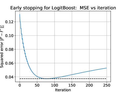
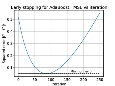
(a)		(b)

Figure 1: Plots of the squared error $\|f^{t}-f^{*}\|_{n}^{2}=\frac{1}{n}\sum_{i=1}^{n}(f^{t}(x_{i})-f^{*}(x_{i}))^{2}$ versus the iteration number $t$ for (a) LogitBoost using a first-order Sobolev kernel (b) AdaBoost using the same first-order Sobolev kernel $\mathbb{K}(x,x^{\prime})=1+\min(x,x^{\prime})$ which generates a class of Lipschitz functions (splines of order one). Both plots correspond to a sample size $n=100$.

In more detail, a broad class of boosting algorithms [24] generate a sequence $\{f^{t}\}_{t=0}^{\infty}$ via updates of the form

$$f^{t+1} =f^{t}-\alpha^{t}g^{t}\quad\text{ with }\quad g^{t}\propto\operatorname*{arg\,max\,}_{\|d\|_{\mathscr{F}}\leq 1}\langle\nabla\mathcal{L}_{n}(f^{t}),\,d(x_{1}^{n})\rangle,$$ (4)

where the scalar $\{\alpha^{t}\}_{t=0}^{\infty}$ is a sequence of step sizes chosen by the user, the constraint $\|d\|_{\mathscr{F}}\leq 1$ defines the unit ball in a given function class $\mathscr{F}$, $\nabla\mathcal{L}_{n}(f)\in^{n}$ denotes the gradient taken at the vector $\big{(}f(x_{1}),\ldots,f(x_{n}))$, and $\langle h,\,g\rangle$ is the usual inner product between vectors $h,g\in^{n}$. For non-decaying step sizes and a convex objective $\mathcal{L}_{n}$, running this procedure for an infinite number of iterations will lead to a minimizer of the empirical loss, thus causing overfitting. In order to illustrate this phenomenon, Figure 1 provides plots of the squared error $\|f^{t}-f^{*}\|_{n}^{2}:\,=\frac{1}{n}\sum_{i=1}^{n}\big{(}f^{t}(x_{i})-f^{*}(x_{i})\big{)}^{2}$ versus the iteration number, for LogitBoost in panel (a) and AdaBoost in panel (b). See Section 4.2 for more details on exactly how these experiments were conducted.

In the plots in Figure 1, the dotted line indicates the minimum mean-squared error $\rho_{n}^{2}$ over all iterates of that particular run of the algorithm. Both plots are qualitatively similar, illustrating the existence of a “good” number of iterations to take, after which the MSE greatly increases. Hence a natural problem is to decide at what iteration $T$ to stop such that the iterate $f^{T}$ satisfies bounds of the form

$$\mathcal{L}(f^{T})-\mathcal{L}(f^{*}) \precsim\rho_{n}^{2}\quad\mbox{and}\quad\|f^{T}-f^{*}\|_{n}^{2}\precsim\rho_{n}^{2}$$ (5)

with high probability. Here $f(n)\precsim g(n)$ indicates that $f(n)\leq cg(n)$ for some universal constant $c\in(0,\infty)$. The main results of this paper provide a stopping rule $T$ for which bounds of the form (5) do in fact hold with high probability over the randomness in the observed responses.

Moreover, as shown by our later results, under suitable regularity conditions, the expectation of the minimum squared error $\rho_{n}^{2}$ is proportional to the statistical minimax risk $\inf_{\widehat{f}}\sup_{f\in\mathcal{F}}\mathbb{E}[\mathcal{L}(\widehat{f})-\mathcal{L}(f)]$, where the infimum is taken over all possible estimators $\widehat{f}$. Note that the minimax risk provides a fundamental lower bound on the performance of any estimator uniformly over the function space $\mathcal{F}$. Coupled with our stopping time guarantee (5), we are guaranteed that our estimate achieves the minimax risk up to constant factors. As a result, our bounds are unimprovable in general (see Corollary 2).

2.2 Reproducing Kernel Hilbert Spaces

The analysis of this paper focuses on algorithms with the update (4) when the function class $\mathscr{F}$ is a reproducing kernel Hilbert space $\mathscr{H}$ (RKHS, see standard sources  [37, 17, 31, 5]), consisting of functions mapping a domain $\mathcal{X}$ to the real line . Any RKHS is defined by a bivariate symmetric kernel function $\mathbb{K}:\mathcal{X}\times\mathcal{X}\rightarrow$ which is required to be positive semidefinite, i.e. for any integer $N\geq 1$ and a collection of points $\{x_{j}\}_{j=1}^{N}$ in $\mathcal{X}$, the matrix $[\mathbb{K}(x_{i},x_{j})]_{ij}\in^{N\times N}$ is positive semidefinite.

The associated RKHS is the closure of the linear span of functions in the form $f(\cdot)=\sum_{j\geq 1}\omega_{j}\mathbb{K}(\cdot,x_{j})$, where $\{x_{j}\}_{j=1}^{\infty}$ is some collection of points in $\mathcal{X}$, and $\{\omega_{j}\}_{j=1}^{\infty}$ is a real-valued sequence. For two functions $f_{1},f_{2}\in\mathscr{H}$ which can be expressed as a finite sum $f_{1}(\cdot)=\sum_{i=1}^{\ell_{1}}\alpha_{i}\mathbb{K}(\cdot,x_{i})$ and $f_{2}(\cdot)=\sum_{j=1}^{\ell_{2}}\beta_{j}\mathbb{K}(\cdot,x_{j})$, the inner product is defined as $\langle f_{1},f_{2}\rangle_{\mathscr{H}}=\sum_{i=1}^{\ell_{1}}\sum_{j=1}^{\ell_{2}}\alpha_{i}\beta_{j}\mathbb{K}(x_{i},x_{j})$ with induced norm $\|f_{1}\|_{\mathscr{H}}^{2}=\sum_{i=1}^{\ell_{1}}\alpha_{i}^{2}\mathbb{K}(x_{i},x_{i})$. For each $x\in\mathcal{X}$, the function $\mathbb{K}(\cdot,x)$ belongs to $\mathscr{H}$, and satisfies the reproducing relation

$$\langle f,\,\mathbb{K}(\cdot,x)\rangle_{\mathscr{H}}=f(x)~{}~{}\text{ for all }f\in\mathscr{H}.$$ (6)

Moreover, when the covariates $X_{i}$ are drawn i.i.d. from a distribution $\mathbb{P}_{X}$ with domain $\mathcal{X}$ we can invoke Mercer’s theorem which states that any function in $\mathscr{H}$ can be represented as

$$\mathbb{K}(x,x^{\prime}) =\sum_{k=1}^{\infty}\mu_{k}\phi_{k}(x)\phi_{k}(x^{\prime}),$$ (7)

where $\mu_{1}\geq\mu_{2}\geq\dots\geq 0$ are the eigenvalues of the kernel function $\mathbb{K}$ and $\{\phi_{k}\}_{k=1}^{\infty}$ are eigenfunctions of $\mathbb{K}$ which form an orthonormal basis of $L^{2}(\mathcal{X},\mathbb{P}_{X})$ with the inner product $\langle f,g\rangle:\,=\int_{\mathcal{X}}f(x)g(x)\text{d}\mathbb{P}_{X}(x)$. We refer the reader to the standard sources [37, 17, 31, 5] for more details on RKHSs and their properties.

Throughout this paper, we assume that the kernel function is uniformly bounded, meaning that there is a constant $L$ such that $\sup_{x\in\mathcal{X}}\mathbb{K}(x,x)\leq L$. Such a boundedness condition holds for many kernels used in practice, including the Gaussian, Laplacian, Sobolev, other types of spline kernels, as well as any trace class kernel with trigonometric eigenfunctions. By rescaling the kernel as necessary, we may assume without loss of generality that $L=1$. As a consequence, for any function $f$ such that $\|f\|_{\mathscr{H}}\leq r$, we have by the reproducing relation that

$$\|f\|_{\infty}=\sup_{x}\langle f,\mathbb{K}(\cdot,x)\rangle_{\mathscr{H}}\leq\|f\|_{\mathscr{H}}\sup_{x}\|\mathbb{K}(\cdot,x)\|_{\mathscr{H}}\leq r.$$

Given samples $\{(x_{i},y_{i})\}_{i=1}^{n}$, by the representer theorem [20], it is sufficient to restrict ourselves to the linear subspace $\mathscr{H}_{n}=\makebox[0.0pt][l]{\hskip 1.29167pt\hskip 0.58333pt\rule[5.59721pt]{17.27151pt}{0.43057pt}}{\text{span}}\{\mathbb{K}(\cdot,x_{i})\}_{i=1}^{n}$, for which all $f\in\mathscr{H}_{n}$ can be expressed as

$$f =\frac{1}{\sqrt{n}}\sum_{i=1}^{n}\omega_{i}\mathbb{K}(\cdot,x_{i})$$ (8)

for some coefficient vector $\omega\in^{n}$. Among those functions which achieve the infimum in expression (1), let us define $f^{*}$ as the one with the minimum Hilbert norm. This definition is equivalent to restricting $f^{*}$ to be in the linear subspace $\mathscr{H}_{n}$.

2.3 Boosting in kernel spaces

For a finite number of covariates $x_{i}$ from $i=1\dots n$, let us define the normalized kernel matrix $K\in^{n\times n}$ with entries $K_{ij}=\mathbb{K}(x_{i},x_{j})/n$. Since we can restrict the minimization of $\mathcal{L}_{n}$ and $\mathcal{L}$ from $\mathscr{H}$ to the subspace $\mathscr{H}_{n}$ w.l.o.g., using expression (8) we can then write the function value vectors $f(x_{1}^{n}):\,=(f(x_{1}),\dots,f(x_{n}))$ as $f(x_{1}^{n})=\sqrt{n}K\omega$. As there is a one-to-one correspondence between the $n$-dimensional vectors $f(x_{1}^{n})\in^{n}$ and the corresponding function $f\in\mathscr{H}_{n}$ in $\mathscr{H}$ by the representer theorem, minimization of an empirical loss in the subspace $\mathscr{H}_{n}$ essentially becomes the $n$-dimensional problem of fitting a response vector $y$ over the set $\operatorname{range}(K)$. In the sequel, all updates will thus be performed on the function value vectors $f(x_{1}^{n})$.

With a change of variable $d(x_{1}^{n})=\sqrt{n}\sqrt{K}z$ we then have

$$d^{t}(x_{1}^{n}) :\,=\operatorname*{arg\,max\,}\limits_{\begin{subarray}{c}\|d\|_{\mathscr{H}}\leq 1\\ d\in\operatorname{range}(K)\end{subarray}}\langle\nabla\mathcal{L}_{n}(f^{t}),\,d(x_{1}^{n})\rangle=\frac{\sqrt{n}K\nabla\mathcal{L}_{n}(f^{t})}{\sqrt{\nabla\mathcal{L}_{n}(f^{t})K\nabla\mathcal{L}_{n}(f^{t})}}.$$

In this paper, we study the choice $g^{t}=\langle\nabla\mathcal{L}_{n}(f^{t}),\,d^{t}(x_{1}^{n})\rangle d^{t}$ in the boosting update (4), so that the function value iterates take the form

$$f^{t+1}(x_{1}^{n}) =f^{t}(x_{1}^{n})-\alpha nK\nabla\mathcal{L}_{n}(f^{t}),$$ (9)

where $\alpha>0$ is a constant stepsize choice. Choosing $f^{0}(x_{1}^{n})=0$ ensures that all iterates $f^{t}(x_{1}^{n})$ remain in the range space of $K$.

In this paper we consider the following three error measures for an estimator $\widehat{f}$:

$$L^{2}(\mathbb{P}_{n})\text{ norm: }~{}~{}~{} \|\widehat{f}-f^{*}\|_{n}^{2}=\frac{1}{n}\sum_{i=1}^{n}\big{(}\widehat{f}(x_{i})-f^{*}(x_{i})\big{)}^{2},$$

$$L^{2}(\mathbb{P}_{X})\text{ norm: }~{}~{}~{} \|\widehat{f}-f^{*}\|_{2}^{2}:\,=\mathbb{E}\big{(}\widehat{f}(X)-f^{*}(X)\big{)}^{2},$$

Excess risk: $$\mathcal{L}(\widehat{f})-\mathcal{L}(f^{*}),$$

where the expectation in the $L^{2}(\mathbb{P}_{X})$-norm is taken over random covariates $X$ which are independent of the samples $(X_{i},Y_{i})$ used to form the estimate $\widehat{f}$. Our goal is to propose a stopping time $T$ such that the averaged function $\widehat{f}=\frac{1}{T}\sum_{t=1}^{T}f^{t}$ satisfies bounds of the type (5). We begin our analysis by focusing on the empirical $L^{2}(\mathbb{P}_{n})$ error, but as we will see in Corollary 1, bounds on the empirical error are easily transformed to bounds on the population $L^{2}(\mathbb{P}_{X})$ error. Importantly, we exhibit such bounds with a statistical error term $\delta_{n}$ that is specified by the localized Gaussian complexity of the kernel class.

3 Main results

We now turn to the statement of our main results, beginning with the introduction of some regularity assumptions.

3.1 Assumptions

Recall from our earlier set-up that we differentiate between the empirical loss function $\mathcal{L}_{n}$ in expression (3), and the population loss $\mathcal{L}$ in expression (1). Apart from assuming differentiability of both functions, all of our remaining conditions are imposed on the population loss. Such conditions at the population level are weaker than their analogues at the empirical level.

For a given radius $r>0$, let us define the Hilbert ball around the optimal function $f^{*}$ as

$$\mathbb{B}_{\mathscr{H}}(f^{*},r):\,=\{f\in\mathscr{H}\mid\|f-f^{*}\|_{\mathscr{H}}\leq r\}.$$ (10)

Our analysis makes particular use of this ball defined for the radius $C_{\mathscr{H}}^{2}:\,=2\max\{\|f^{*}\|_{\mathscr{H}}^{2},~{}32,\sigma^{2}\}$ where the effective noise level $\sigma$ is defined in the sequel.

We assume that the population loss is $m$-strongly convex and $M$-smooth over $\mathbb{B}_{\mathscr{H}}(f^{*},2C_{\mathscr{H}})$, meaning that the
$m$-$M$-condition:

$$\frac{m}{2}\|f-g\|_{n}^{2}\leq\mathcal{L}(f)-\mathcal{L}(g)- \langle\nabla\mathcal{L}(g),\,f(x_{1}^{n})-g(x_{1}^{n})\rangle$$

$$\hskip 42.67912pt\leq\frac{M}{2}\|f-g\|_{n}^{2}$$

holds for all $f,g\in\mathbb{B}_{\mathscr{H}}(f^{*},2C_{\mathscr{H}})$ and all design points $\{x_{i}\}_{i=1}^{n}$. In addition, we assume that the function $\phi$ is $M$-Lipschitz in its second argument over the interval $\theta\in[\min\limits_{i\in[n]}f^{*}(x_{i})-2C_{\mathscr{H}},\max\limits_{i\in[n]}f^{*}(x_{i})+2C_{\mathscr{H}}]$. To be clear, here $\nabla\mathcal{L}(g)$ denotes the vector in ⁿ obtained by taking the gradient of $\mathcal{L}$ with respect to the vector $g(x_{1}^{n})$. It can be verified by a straightforward computation that when $\mathcal{L}$ is induced by the least-squares cost $\phi(y,\theta)=\frac{1}{2}(y-\theta)^{2}$, the $m$-$M$-condition  holds for $m=M=1$. The logistic and exponential loss satisfy this condition (see supp. material), where it is key that we have imposed the condition only locally on the ball $\mathbb{B}_{\mathscr{H}}(f^{*},2C_{\mathscr{H}})$.

In addition to the least-squares cost, our theory also applies to losses $\mathcal{L}$ induced by scalar functions $\phi$ that satisfy the
$\phi^{\prime}$-boundedness:

$$\max_{i=1,\ldots,n}\left|\frac{\partial\phi(y,\theta)}{\partial\theta}\right|_{\theta=f(x_{i})}\leq B$$

$$\hskip 28.45274pt\mbox{ for all $f\in\mathbb{B}_{\mathscr{H}}(f^{*},2C_{\mathscr{H}})$ and }y\in\mathcal{Y}.$$

This condition holds with $B=1$ for the logistic loss for all $\mathcal{Y}$, and $B=\exp(2.5C_{\mathscr{H}})$ for the exponential loss for binary classification with $\mathcal{Y}=\{-1,1\}$, using our kernel boundedness condition. Note that whenever this condition holds with some finite $B$, we can always rescale the scalar loss $\phi$ by $1/B$ so that it holds with $B=1$, and we do so in order to simplify the statement of our results.

3.2 Upper bound in terms of localized Gaussian width

Our upper bounds involve a complexity measure known as the localized Gaussian width. In general, Gaussian widths are widely used to obtain risk bounds for least-squares and other types of $M$-estimators. In our case, we consider Gaussian complexities for “localized” sets of the form

$$\mathcal{E}_{n}(\delta,1):\,=\Big{\{}f-g\mid\|f-g\|_{\mathscr{H}}\leq 1,~{}\|f-g\|_{n}\leq\delta\Big{\}}$$ (11)

with $f,g\in\mathscr{H}$. The Gaussian complexity localized at scale $\delta$ is given by

$$\mathcal{G}_{n}\big{(}\mathcal{E}_{n}(\delta,1)\big{)} :\,=\mathbb{E}\Big{[}\sup_{g\in\mathcal{E}_{n}(\delta,1)}\frac{1}{n}\sum_{i=1}^{n}w_{i}g(x_{i})\Big{]},$$ (12)

where $(w_{1},\ldots,w_{n})$ denotes an i.i.d. sequence of standard Gaussian variables.

An essential quantity in our theory is specified by a certain fixed point equation that is now standard in empirical process theory [33, 3, 21, 27]. Let us define the effective noise level

$$\sigma :\,=\begin{cases}\min\Big{\{}t\,\mid\,\max\limits_{i=1,\ldots,n}\mathbb{E}[e^{((Y_{i}-f^{*}(x_{i}))^{2}/t^{2})}]<\infty\Big{\}}~{}~{}\mbox{for L.S.}\\ 4\,(2M+1)(1+2C_{\mathscr{H}})~{}~{}\mbox{for $\phi^{\prime}$-bounded losses.}\end{cases}$$ (13)

The critical radius $\delta_{n}$ is the smallest positive scalar such that

$$\frac{\mathcal{G}_{n}(\mathcal{E}_{n}(\delta,1))}{\delta}~{}\leq~{}\frac{\delta}{\sigma}.$$ (14)

We note that past work on localized Rademacher and Gaussian complexity [25, 3] guarantees that there exists a unique $\delta_{n}>0$ that satisfies this condition, so that our definition is sensible.

3.2.1 Upper bounds on excess risk and empirical $L^{2}(\mathbb{P}_{n})$-error

With this set-up, we are now equipped to state our main theorem. It provides high-probability bounds on the excess risk and $L^{2}(\mathbb{P}_{n})$-error of the estimator $\bar{f}^{T}:\,=\frac{1}{T}\sum_{t=1}^{T}f^{t}$ defined by averaging the $T$ iterates of the algorithm. It applies to both the least-squares cost function, and more generally, to any loss function satisfying the $m$-$M$-condition and the $\phi^{\prime}$-boundedness condition.

Theorem 1.

Suppose that the sample size $n$ large enough such that $\delta_{n}\leq\frac{M}{m}$, and we compute the sequence $\{f^{t}\}_{t=0}^{\infty}$ using the update (9) with initialization $f^{0}=0$ and any step size $\alpha\in(0,\min\{\frac{1}{M},M\}]$. Then for any iteration $T\in\big{\{}0,1,\ldots\lfloor\frac{m}{8M\delta_{n}^{2}}\rfloor\big{\}}$, the averaged function estimate $\bar{f}^{T}$ satisfies the bounds

$$\mathcal{L}(\bar{f}^{T})-\mathcal{L}(f^{*}) \leq CM\Big{(}\frac{1}{\alpha mT}+\frac{\delta_{n}^{2}}{m^{2}}\Big{)},\quad\mbox{and}$$ (15a)

$$\|\bar{f}^{T}-f^{*}\|_{n}^{2} \leq C\Big{(}\frac{1}{\alpha mT}+\frac{\delta_{n}^{2}}{m^{2}}\Big{)},$$ (15b)

where both inequalities hold with probability at least $1-c_{1}\exp(-C_{2}\frac{m^{2}n\delta_{n}^{2}}{\sigma^{2}})$.

We prove Theorem 1 in Section 5.1.

A few comments about the constants in our statement: in all cases, constants of the form $c_{j}$ are universal, whereas the capital $C_{j}$ may depend on parameters of the joint distribution and population loss $\mathcal{L}$. In Theorem 1, we have the explicit value $C_{2}=\{\frac{m^{2}}{\sigma^{2}},1\}$ and $C^{2}$ is proportional to the quantity $2\max\{\|f^{*}\|_{\mathscr{H}}^{2},~{}32,~{}\sigma^{2}\}$. While inequalities (15a) and (15b) are stated as high probability results, similar bounds for expected loss (over the response $y_{i}$, with the design fixed) can be obtained by a simple integration argument.

In order to gain intuition for the claims in the theorem, note that apart from factors depending on $(m,M)$, the first term $\frac{1}{\alpha mT}$ dominates the second term $\frac{\delta_{n}^{2}}{m^{2}}$ whenever $T\lesssim 1/\delta_{n}^{2}$. Consequently, up to this point, taking further iterations reduces the upper bound on the error. This reduction continues until we have taken of the order $1/\delta_{n}^{2}$ many steps, at which point the upper bound is of the order $\delta_{n}^{2}$.

More precisely, suppose that we perform the updates with step size $\alpha=\frac{m}{M}$; then, after a total number of $\tau:\,=\frac{1}{\delta_{n}^{2}\max\{8,M\}}$ many iterations, the extension of Theorem 1 to expectations guarantees that the mean squared error is bounded as

$$\mathbb{E}\|\bar{f}^{\tau}-f^{*}\|_{n}^{2} \leq C^{\prime}\;\frac{\delta_{n}^{2}}{m^{2}},$$ (16)

where $C^{\prime}$ is another constant depending on $C_{\mathscr{H}}$. Here we have used the fact that $M\geq m$ in simplifying the expression. It is worth noting that guarantee (16) matches the best known upper bounds for kernel ridge regression (KRR)—indeed, this must be the case, since a sharp analysis of KRR is based on the same notion of localized Gaussian complexity (e.g. [2, 3]) . Thus, our results establish a strong parallel between the algorithmic regularization of early stopping, and the penalized regularization of kernel ridge regression. Moreover, as will be clarified in Section 3.3, under suitable regularity conditions on the RKHS, the critical squared radius $\delta_{n}^{2}$ also acts as a lower bound for the expected risk, meaning that our upper bounds are not improvable in general.

Note that the critical radius $\delta_{n}^{2}$ only depends on our observations $\{(x_{i},y_{i})\}_{i=1}^{n}$ through the solution of inequality (14). In many cases, it is possible to compute and/or upper bound this critical radius, so that a concrete and valid stopping rule can indeed by calculated in advance. In Section 4, we provide a number of settings in which this can be done in terms of the eigenvalues $\{\mu_{j}\}_{j=1}^{n}$ of the normalized kernel matrix.

3.2.2 Consequences for random design regression

Thus far, our analysis has focused purely on the case of fixed design, in which the sequence of covariates $\{x_{i}\}_{i=1}^{n}$ is viewed as fixed. If we instead view the covariates as being sampled in an i.i.d. manner from some distribution $\mathbb{P}_{X}$ over $\mathcal{X}$, then the empirical error $\|\widehat{f}-f^{*}\|_{n}^{2}=\frac{1}{n}\sum_{i=1}^{n}\big{(}f(x_{i})-f^{*}(x_{i})\big{)}^{2}$ of a given estimate $\widehat{f}$ is a random quantity, and it is interesting to relate it to the squared population $L^{2}(\mathbb{P}_{X})$-norm $\|\widehat{f}-f^{*}\|_{2}^{2}=\mathbb{E}\big{[}(\widehat{f}(X)-f^{*}(X))^{2}\big{]}$.

In order to state an upper bound on this error, we introduce a population analogue of the critical radius $\delta_{n}$, which we denote by $\makebox[0.0pt][l]{\hskip 2.08334pt\rule[8.23611pt]{2.24303pt}{0.43057pt}}{\delta}_{n}$. Consider the set

$$\makebox[0.0pt][l]{\hskip 2.05pt\rule[8.12498pt]{4.51776pt}{0.43057pt}}{\mathcal{E}}(\delta,1) :\,=\Big{\{}f-g\,\mid\,f,g\in\mathscr{H},~{}\|f-g\|_{\mathscr{H}}\leq 1,~{}\|f-g\|_{2}\leq\delta\Big{\}}.$$ (17)

It is analogous to the previously defined set $\mathcal{E}(\delta,1)$, except that the empirical norm $\|\cdot\|_{n}$ has been replaced by the population version. The population Gaussian complexity localized at scale $\delta$ is given by

$$\mathcal{\makebox[0.0pt][l]{\hskip 2.05pt\rule[8.12498pt]{5.52184pt}{0.43057pt}}{G}}_{n}\big{(}\makebox[0.0pt][l]{\hskip 2.05pt\rule[8.12498pt]{4.51776pt}{0.43057pt}}{\mathcal{E}}(\delta,1)\big{)} :\,=\mathbb{E}_{w,X}\Big{[}\sup_{g\in\makebox[0.0pt][l]{\hskip 1.435pt\rule[5.6875pt]{3.16245pt}{0.3014pt}}{\mathcal{E}}(\delta,1)}\frac{1}{n}\sum_{i=1}^{n}w_{i}g(X_{i})\Big{]},$$ (18)

where $\{w_{i}\}_{i=1}^{n}$ are an i.i.d. sequence of standard normal variates, and $\{X_{i}\}_{i=1}^{n}$ is a second i.i.d. sequence, independent of the normal variates, drawn according to $\mathbb{P}_{X}$. Finally, the population critical radius $\makebox[0.0pt][l]{\hskip 2.08334pt\rule[8.23611pt]{2.24303pt}{0.43057pt}}{\delta}_{n}$ is defined by equation (18), in which $\mathcal{G}_{n}$ is replaced by $\mathcal{\makebox[0.0pt][l]{\hskip 2.05pt\rule[8.12498pt]{5.52184pt}{0.43057pt}}{G}}_{n}$.

Corollary 1.

In addition to the conditions of Theorem 1, suppose that the sequence $\{(X_{i},Y_{i})\}_{i=1}^{n}$ of covariate-response pairs are drawn i.i.d. from some joint distribution $\mathbb{P}$, and we compute the boosting updates with step size $\alpha\in(0,\min\{\frac{1}{M},M\}]$ and initialization $f^{0}=0$. Then the averaged function estimate $\bar{f}^{T}$ at time $T:\,=\lfloor\frac{1}{\delta_{n}^{2}\max\{8,M\}}\rfloor$ satisfies the bound

$$\mathbb{E}_{X}\big{(}\bar{f}^{T}(X)-f^{*}(X)\big{)}^{2}\;=\;\|\bar{f}^{T}-f^{*}\|_{2}^{2}\leq\tilde{c}\;\makebox[0.0pt][l]{\hskip 2.08334pt\rule[8.23611pt]{2.24303pt}{0.43057pt}}{\delta}_{n}^{2}$$

with probability at least $1-c_{1}\exp(-C_{2}\frac{m^{2}n\delta_{n}^{2}}{\sigma^{2}})$ over the random samples.

The proof of Corollary 1 follows directly from standard empirical process theory bounds [3, 27] on the difference between empirical risk $\|\bar{f}^{T}-f^{*}\|_{n}^{2}$ and population risk $\|\bar{f}^{T}-f^{*}\|_{2}^{2}$. In particular, it can be shown that $\|\cdot\|_{2}$ and $\|\cdot\|_{n}$ norms differ only by a factor proportion to $\makebox[0.0pt][l]{\hskip 2.08334pt\rule[8.23611pt]{2.24303pt}{0.43057pt}}{\delta}_{n}$. Furthermore, one can show that the empirical critical quantity $\delta_{n}$ is bounded by the population $\makebox[0.0pt][l]{\hskip 2.08334pt\rule[8.23611pt]{2.24303pt}{0.43057pt}}{\delta}_{n}$. By combining both arguments the corollary follows. We refer the reader to the papers [3, 27] for further details on such equivalences.

It is worth comparing this guarantee with the past work of Raskutti et al. [27], who analyzed the kernel boosting iterates of the form (9), but with attention restricted to the special case of the least-squares loss. Their analysis was based on first decomposing the squared error into bias and variance terms, then carefully relating the combination of these terms to a particular bound on the localized Gaussian complexity (see equation (19) below). In contrast, our theory more directly analyzes the effective function class that is explored by taking $T$ steps, so that the localized Gaussian width (18) appears more naturally. In addition, our analysis applies to a broader class of loss functions.

In the case of reproducing kernel Hilbert spaces, it is possible to sandwich the localized Gaussian complexity by a function of the eigenvalues of the kernel matrix. Mendelson [25] provides this argument in the case of the localized Rademacher complexity, but similar arguments apply to the localized Gaussian complexity. Letting $\mu_{1}\geq\mu_{2}\geq\cdots\geq\mu_{n}\geq 0$ denote the ordered eigenvalues of the normalized kernel matrix $K$, define the function

$$\mathcal{R}(\delta) =\frac{1}{\sqrt{n}}\sqrt{\sum_{j=1}^{n}\min\{\delta^{2},\mu_{j}\}}.$$ (19)

Up to a universal constant, this function is an upper bound on the Gaussian width $\mathcal{G}_{n}\big{(}\mathcal{E}(\delta,1)\big{)}$ for all $\delta\geq 0$, and up to another universal constant, it is also a lower bound for all $\delta\geq\frac{1}{\sqrt{n}}$.

3.3 Achieving minimax lower bounds

In this section, we show that the upper bound (16) matches known minimax lower bounds on the error, so that our results are unimprovable in general. We establish this result for the class of regular kernels, as previously defined by Yang et al. [39], which includes the Gaussian and Sobolev kernels as special cases.

The class of regular kernels is defined as follows. Let $\mu_{1}\geq\mu_{2}\geq\cdots\geq\mu_{n}\geq 0$ denote the ordered eigenvalues of the normalized kernel matrix $K$, and define the quantity $d_{n}:\,=\operatorname{argmin}_{j=1,\dots,n}\{\mu_{j}\leq\delta_{n}^{2}\}$. A kernel is called regular whenever there is a universal constant $c$ such that the tail sum satisfies $\sum_{j=d_{n}+1}^{n}\mu_{j}\leq c\,d_{n}\delta_{n}^{2}$. In words, the tail sum of the eigenvalues for regular kernels is roughly on the same or smaller scale as the sum of the eigenvalues bigger than $\delta_{n}^{2}$.

For such kernels and under the Gaussian observation model ($Y_{i}\sim N(f^{*}(x_{i}),\sigma^{2})$), Yang et al. [39] prove a minimax lower bound involving $\delta_{n}$. In particular, they show that the minimax risk over the unit ball of the Hilbert space is lower bounded as

$$\inf_{\widehat{f}}\sup_{\|f^{*}\|_{\mathscr{H}}\leq 1}\mathbb{E}\|\widehat{f}-f^{*}\|_{n}^{2}\geq c_{\ell}\delta_{n}^{2}.$$ (20)

Comparing the lower bound (20) with upper bound (16) for our estimator $\bar{f}^{T}$ stopped after $O(1/\delta_{n}^{2})$ many steps, it follows that the bounds proven in Theorem 1 are unimprovable apart from constant factors.

We now state a generalization of this minimax lower bound, one which applies to a sub-class of generalized linear models, or GLM for short. In these models, the conditional distribution of the observed vector $Y=(Y_{1},\ldots,Y_{n})$ given $\big{(}f^{*}(x_{1}),\ldots,f^{*}(x_{n})\big{)}$ takes the form

$$\mathbb{P}_{\theta}(y)=\prod_{i=1}^{n}\Big{[}h(y_{i})\exp\big{(}\frac{y_{i}f^{*}(x_{i})-\Phi(f^{*}(x_{i}))}{s(\sigma)}\big{)}\Big{]},$$ (21)

where $s(\sigma)$ is a known scale factor and $\Phi:\to$ is the cumulant function of the generalized linear model. As some concrete examples:

• The linear Gaussian model is recovered by setting $s(\sigma)=\sigma^{2}$ and $\Phi(t)=t^{2}/2$.

• The logistic model for binary responses $y\in\{-1,1\}$ is recovered by setting $s(\sigma)=1$ and $\Phi(t)=\log(1+\exp(t))$.

Our minimax lower bound applies to the class of GLMs for which the cumulant function $\Phi$ is differentiable and has uniformly bounded second derivative $|\Phi^{\prime\prime}|\leq L$. This class includes the linear, logistic, multinomial families, among others, but excludes (for instance) the Poisson family. Under this condition, we have the following:

Corollary 2.

Suppose that we are given i.i.d. samples $\{y_{i}\}_{i=1}^{n}$ from a GLM (21) for some function $f^{*}$ in a regular kernel class with $\|f^{*}\|_{\mathscr{H}}\leq 1$. Then running $T:\,=\lfloor\frac{1}{\delta_{n}^{2}\max\{8,M\}}\rfloor$ iterations with step size $\alpha\in(0,\min\{\frac{1}{M},M\}]$ and $f^{0}=0$ yields an estimate $\bar{f}^{T}$ such that

$$\mathbb{E}\|\bar{f}^{T}-f^{*}\|_{n}^{2} \,\asymp\,\inf_{\widehat{f}}\sup_{\|f^{*}\|_{\mathscr{H}}\leq 1}\mathbb{E}\|\widehat{f}-f^{*}\|_{n}^{2}.$$ (22)

Here $f(n)\asymp g(n)$ means $f(n)=cg(n)$ up to a universal constant $c\in(0,\infty)$. As always, in the minimax claim (22), the infimum is taken over all measurable functions of the input data and the expectation is taken over the randomness of the response variables $\{Y_{i}\}_{i=1}^{n}$. Since we know that $\mathbb{E}\|\bar{f}^{T}-f^{*}\|_{n}^{2}\precsim\delta_{n}^{2}$, the way to prove bound (22) is by establishing $\inf_{\widehat{f}}\sup_{\|f^{*}\|_{\mathscr{H}}\leq 1}\mathbb{E}\|\widehat{f}-f^{*}\|_{n}^{2}\succsim\delta_{n}^{2}$. See Section 5.2 for the proof of this result.

At a high level, the statement in Corollary 2 shows that early stopping prevents us from overfitting to the data; in particular, using the stopping time $T$ yields an estimate that attains the optimal balance between bias and variance.

4 Consequences for various kernel classes

In this section, we apply Theorem 1 to derive some concrete rates for different kernel spaces and then illustrate them with some numerical experiments. It is known that the complexity of an RKHS in association with a distribution over the covariates $\mathbb{P}_{X}$ can be characterized by the decay rate (7) of the eigenvalues of the kernel function. In the finite sample setting, the analogous quantities are the eigenvalues $\{\mu_{j}\}_{j=1}^{n}$ of the normalized kernel matrix $K$. The representation power of a kernel class is directly correlated with the eigen-decay: the faster the decay, the smaller the function class. When the covariates are drawn from the distribution $\mathbb{P}_{X}$, empirical process theory guarantees that the empirical and population eigenvalues are close.

4.1 Theoretical predictions as a function of decay

In this section, let us consider two broad types of eigen-decay:

• $\gamma$-exponential decay: For some $\gamma>0$, the kernel matrix eigenvalues satisfy a decay condition of the form $\mu_{j}\leq c_{1}\exp(-c_{2}j^{\gamma})$, where $c_{1},c_{2}$ are universal constants. Examples of kernels in this class include the Gaussian kernel, which for the Lebesgue measure satisfies such a bound with $\gamma=2$ (real line) or $\gamma=1$ (compact domain).

• $\beta$-polynomial decay: For some $\beta>1/2$, the kernel matrix eigenvalues satisfy a decay condition of the form $\mu_{j}\leq c_{1}j^{-2\beta}$, where $c_{1}$ is a universal constant. Examples of kernels in this class include the $k^{th}$-order Sobolev spaces for some fixed integer $k\geq 1$ with Lebesgue measure on a bounded domain. We consider Sobolev spaces that consist of functions that have $k^{th}$-order weak derivatives $f^{(k)}$ being Lebesgue integrable and $f(0)=f^{(1)}(0)=\dots=f^{(k-1)}(0)=0$. For such classes, the $\beta$-polynomial decay condition holds with $\beta=k$.

Given eigendecay conditions of these types, it is possible to compute an upper bound on the critical radius $\delta_{n}$. In particular, using the fact that the function $\mathcal{R}$ from equation (19) is an upper bound on the function $\mathcal{G}_{n}\big{(}\mathcal{E}(\delta,1)\big{)}$, we can show that for $\gamma$-exponentially decaying kernels, we have $\delta_{n}^{2}\precsim\frac{(\log n)^{1/\gamma}}{n}$, whereas for $\beta$-polynomial kernels, we have $\delta_{n}^{2}\precsim n^{-\frac{2\beta}{2\beta+1}}$ up to universal constants. Combining with our Theorem 1, we obtain the following result:

Corollary 3 (Bounds based on eigendecay).

Under the conditions of Theorem 1:

1. For kernels with $\gamma$-exponential eigen-decay, we have

   $$\mathbb{E}\|\bar{f}^{T}-f^{*}\|_{n}^{2}\leq c\,\frac{\log^{1/\gamma}n}{n}~{}~{}\mbox{at $T\asymp\frac{n}{\log^{1/\gamma}n}$ steps.}$$ (23a)

2. For kernels with $\beta$-polynomial eigen-decay, we have

   $$\mathbb{E}\|\bar{f}^{T}-f^{*}\|_{n}^{2}\leq c\,n^{-2\beta/(2\beta+1)}~{}~{}\mbox{at $T\asymp n^{2\beta/(2\beta+1)}$ steps.}$$ (23b)

See Section 5.3 for the proof of Corollary 3.

In particular, these bounds hold for LogitBoost and AdaBoost. We note that similar bounds can also be derived with regard to risk in $L^{2}(\mathbb{P}_{n})$ norm as well as the excess risk $\mathcal{L}(f^{T})-\mathcal{L}(f^{*})$.

To the best of our knowledge, this result is the first to show non-asymptotic and optimal statistical rates for the $\|\cdot\|_{n}^{2}$-error when early stopping LogitBoost or AdaBoost with an explicit dependence of the stopping rule on $n$. Our results also yield similar guarantees for $L^{2}$-boosting, as has been established in past work [27]. Note that we can observe a similar trade-off between computational efficiency and statistical accuracy as in the case of kernel least-squares regression [40, 27]: although larger kernel classes (e.g. Sobolev classes) yield higher estimation errors, boosting updates reach the optimum faster than for a smaller kernel class (e.g. Gaussian kernels).

4.2 Numerical experiments

We now describe some numerical experiments that provide illustrative confirmations of our theoretical predictions. While we have applied our methods to various kernel classes, in this section, we present numerical results for the first-order Sobolev kernel as two typical examples for exponential and polynomial eigen-decay kernel classes.

Let us start with the first-order Sobolev space of Lipschitz functions on the unit interval $[0,1]$, defined by the kernel $\mathbb{K}(x,x^{\prime})=1+\min(x,x^{\prime})$, and with the design points $\{x_{i}\}_{i=1}^{n}$ set equidistantly over $[0,1]$. Note that the equidistant design yields $\beta$-polynomial decay of the eigenvalues of $K$ with $\beta=1$ as in the case when $x_{i}$ are drawn i.i.d. from the uniform measure on $[0,1]$. Consequently we have that $\delta_{n}^{2}\asymp n^{-2/3}$. Accordingly, our theory predicts that the stopping time $T=(cn)^{2/3}$ should lead to an estimate $\bar{f}^{T}$ such that $\|\bar{f}^{T}-f^{*}\|_{n}^{2}\precsim n^{-2/3}$.

In our experiments for $L^{2}$-Boost, we sampled $Y_{i}$ according to $Y_{i}=f^{*}(x_{i})+w_{i}$ with $w_{i}\sim\mathcal{N}(0,0.5)$, which corresponds to the probability distribution $\mathbb{P}(Y\mid x_{i})=\mathcal{N}(f^{*}(x_{i});0.5)$, where $f^{*}(x)=|x-\frac{1}{2}|-\frac{1}{4}$ is defined on the unit interval $[0,1]$. By construction, the function $f^{*}$ belongs to the first-order Sobolev space with $\|f^{*}\|_{\mathscr{H}}=1$. For LogitBoost, we sampled $Y_{i}$ according to $\text{Bin}(p(x_{i}),5)$ where $p(x)=\frac{\exp(f^{*}(x))}{1+\exp(f^{*}(x))}$. In all cases, we fixed the initialization $f^{0}=0$, and ran the updates (9) for $L^{2}$-Boost and LogitBoost with the constant step size $\alpha=0.75$. We compared various stopping rules to the oracle gold standard $G$, meaning the procedure that examines all iterates $\{f^{t}\}$, and chooses the stopping time $G=\arg\min_{t\geq 1}\|f^{t}-f^{*}\|_{n}^{2}$ that yields the minimum prediction error. Of course, this procedure is unimplementable in practice, but it serves as a convenient lower bound with which to compare.

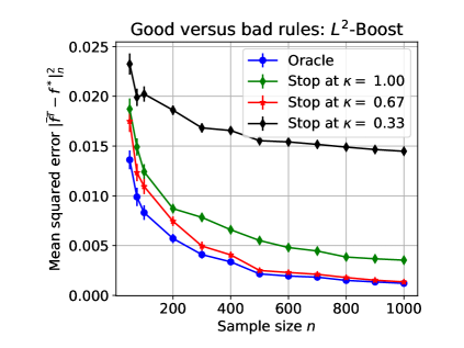
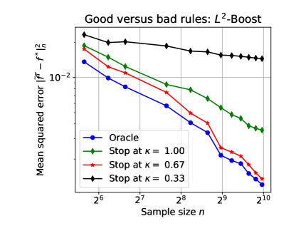
(a)		(b)

Figure 2: The mean-squared errors for the stopped iterates $\bar{f}^{T}$ at the Gold standard, i.e. iterate with the minimum error among all unstopped updates (blue) and at $T=(7n)^{\kappa}$ (with the theoretically optimal $\kappa=0.67$ in red, $\kappa=0.33$ in black and $\kappa=1$ in green) for (a) $L^{2}$-Boost and (b) LogitBoost.

Figure 2 shows plots of the mean-squared error $\|\bar{f}^{T}-f^{*}\|_{n}^{2}$ over the sample size $n$ averaged over $40$ trials, for the gold standard $T=G$ and stopping rules based on $T=(7n)^{\kappa}$ for different choices of $\kappa$. Error bars correspond to the standard errors computed from our simulations. Panel (a) shows the behavior for $L^{2}$-boosting, whereas panel (b) shows the behavior for LogitBoost.

Note that both plots are qualitatively similar and that the theoretically derived stopping rule $T=(7n)^{\kappa}$ with $\kappa^{*}=2/3=0.67$, while slightly worse than the Gold standard, tracks its performance closely. We also performed simulations for some “bad” stopping rules, in particular for an exponent $\kappa$ not equal to $\kappa^{*}=2/3$, indicated by the green and black curves. In the log scale plots in Figure 3 we can clearly see that for $\kappa\in\{0.33,1\}$ the performance is indeed much worse, with the difference in slope even suggesting a different scaling of the error with the number of observations $n$. Recalling our discussion for Figure 1, this phenomenon likely occurs due to underfitting and overfitting effects. These qualitative shifts are consistent with our theory.

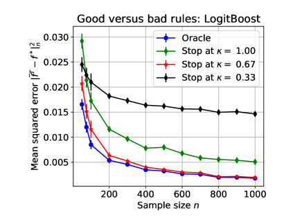
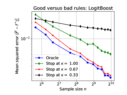
(a)		(b)

Figure 3: Logarithmic plots of the mean-squared errors at the Gold standard in blue and at $T=(7n)^{\kappa}$ (with the theoretically optimal rule for $\kappa=0.67$ in red, $\kappa=0.33$ in black and $\kappa=1$ in green) for (a) $L^{2}$-Boost and (b) LogitBoost.

5 Proof of main results

In this section, we present the proofs of our main results. The technical details are deferred to Appendix A.

In the following, recalling the discussion in Section 2.3, we denote the vector of function values of a function $f\in\mathscr{H}$ evaluated at $(x_{1},x_{2},\ldots,x_{n})$ as $\theta_{f}:\,=f(x_{1}^{n})=(f(x_{1}),f(x_{2}),\ldots f(x_{n}))\in^{n}$, where we omit the subscript $f$ when it is clear from the context. As mentioned in the main text, updates on the function value vectors $\theta^{t}\in^{n}$ correspond uniquely to updates of the functions $f^{t}\in\mathscr{H}$. In the following we repeatedly abuse notation by defining the Hilbert norm and empirical norm on vectors in $\Delta\in\operatorname{range}(K)$ as

$$\|\Delta\|_{\mathscr{H}}^{2}=\frac{1}{n}\Delta^{T}K^{\dagger}\Delta\quad\text{ and }\quad\|\Delta\|_{n}^{2}=\frac{1}{n}\|\Delta\|_{2}^{2},$$

where $K^{\dagger}$ is the pseudoinverse of $K$. We also use $\mathbb{B}_{\mathscr{H}}(\theta,r)$ to denote the ball with respect to the $\|\cdot\|_{\mathscr{H}}$-norm in $\operatorname{range}(K)$.

5.1 Proof of Theorem 1

The proof of our main theorem is based on a sequence of lemmas, all of which are stated with the assumptions of Theorem 1 in force. The first lemma establishes a bound on the empirical norm $\|\cdot\|_{n}$ of the error $\Delta^{t+1}:\,=\theta^{t+1}-\theta^{*}$, provided that its Hilbert norm is suitably controlled.

Lemma 1.

For any stepsize $\alpha\in(0,~{}\frac{1}{M}]$ and any iteration $t$ we have

$$\frac{m}{2}\|\Delta^{t+1}\|_{n}^{2} \leq\frac{1}{2\alpha}\Big{\{}\|\Delta^{t}\|_{\mathscr{H}}^{2}-\|\Delta^{t+1}\|_{\mathscr{H}}^{2}\Big{\}}+\langle\nabla\mathcal{L}(\theta^{*}+\Delta^{t})-\nabla\mathcal{L}_{n}(\theta^{*}+\Delta^{t}),\,\Delta^{t+1}\rangle.$$

See Section A.1 for the proof of this claim.

The second term on the right-hand side of the bound (1) involves the difference between the population and empirical gradient operators. Since this difference is being evaluated at the random points $\Delta^{t}$ and $\Delta^{t+1}$, the following lemma establishes a form of uniform control on this term.

Let us define the set

$$\mathbb{S} :\,=\Biggr{\{}\Delta,\widetilde{\Delta}\in^{n}\mid\|\Delta\|_{\mathscr{H}}\geq 1,~{}\mbox{and}~{}\Delta,~{}\widetilde{\Delta}\in\mathbb{B}_{\mathscr{H}}(0,2C_{\mathscr{H}})\Biggr{\}},$$ (24)

and consider the uniform bound

$$\langle\nabla\mathcal{L}(\theta^{*}+\widetilde{\Delta}) -\nabla\mathcal{L}_{n}(\theta^{*}+\widetilde{\Delta}),\,\Delta\rangle\leq 2\delta_{n}\|\Delta\|_{n}$$

$$+2\delta_{n}^{2}\|\Delta\|_{\mathscr{H}}+\frac{m}{c_{3}}\|\Delta\|_{n}^{2}\quad\mbox{for all $\Delta,\widetilde{\Delta}\in\mathbb{S}$.}$$ (25)

Lemma 2.

Let $\mathcal{E}$ be the event that bound (5.1) holds. There are universal constants $(c_{1},c_{2})$ such that $\mathbb{P}[\mathcal{E}]\geq 1-c_{1}\exp(-c_{2}\frac{m^{2}n\delta_{n}^{2}}{\sigma^{2}})$.

See Section A.2 for the proof of Lemma 2.

Note that Lemma 1 applies only to error iterates with a bounded Hilbert norm. Our last lemma provides this control for some number of iterations:

Lemma 3.

There are constants $(C_{1},C_{2})$ independent of $n$ such that for any step size $\alpha\in\big{(}0,\min\{M,\frac{1}{M}\}\big{]}$, we have

$$\|\Delta^{t}\|_{\mathscr{H}}\leq C_{\mathscr{H}}\qquad\mbox{for all iterations $t\leq\frac{m}{8M\delta_{n}^{2}}$}$$ (26)

with probability at least $1-C_{1}\exp(-C_{2}n\delta_{n}^{2})$, where $C_{2}=\max\{\frac{m^{2}}{\sigma^{2}},1\}$.

See Section A.3 for the proof of this lemma which also uses Lemma 2.

Taking these lemmas as given, we now complete the proof of the theorem. We first condition on the event $\mathcal{E}$ from Lemma 2, so that we may apply the bound (5.1). We then fix some iterate $t$ such that $t<\frac{m}{8M\delta_{n}^{2}}-1$, and condition on the event that the bound (26) in Lemma 3 holds, so that we are guaranteed that $\|\Delta^{t+1}\|_{\mathscr{H}}\leq C_{\mathscr{H}}$. We then split the analysis into two cases:

Case 1

First, suppose that $\|\Delta^{t+1}\|_{n}\leq\delta_{n}C_{\mathscr{H}}$. In this case, inequality (15b) holds directly.

Case 2

Otherwise, we may assume that $\|\Delta^{t+1}\|_{n}>\delta_{n}\|\Delta^{t+1}\|_{\mathscr{H}}$. Applying the bound (5.1) with the choice $(\widetilde{\Delta},\Delta)=(\Delta^{t},\Delta^{t+1})$ yields

$$\langle\nabla\mathcal{L}(\theta^{*}+\Delta^{t}) -\nabla\mathcal{L}_{n}(\theta^{*}+\Delta^{t}),\,\Delta^{t+1}\rangle\leq 4\delta_{n}\|\Delta^{t+1}\|_{n}+\frac{m}{c_{3}}\|\Delta^{t+1}\|_{n}^{2}.$$ (27)

Substituting inequality (27) back into equation (1) yields

$$\frac{m}{2}\|\Delta^{t+1}\|_{n}^{2}\leq\frac{1}{2\alpha}\Big{\{}\|\Delta^{t}\|_{\mathscr{H}}^{2} -\|\Delta^{t+1}\|_{\mathscr{H}}^{2}\Big{\}}+4\delta_{n}\|\Delta^{t+1}\|_{n}+\frac{m}{c_{3}}\|\Delta^{t+1}\|_{n}^{2}.$$

Re-arranging terms yields the bound

$$\gamma m\|\Delta^{t+1}\|_{n}^{2}\leq D^{t}+4\delta_{n}\|\Delta^{t+1}\|_{n},$$ (28)

where we have introduced the shorthand notation $D^{t}:\,=\frac{1}{2\alpha}\Big{\{}\|\Delta^{t}\|_{\mathscr{H}}^{2}-\|\Delta^{t+1}\|_{\mathscr{H}}^{2}\Big{\}}$, as well as $\gamma=\frac{1}{2}-\frac{1}{c_{3}}$

Equation (28) defines a quadratic inequality with respect to $\|\Delta^{t+1}\|_{n}$; solving it and making use of the inequality $(a+b)^{2}\leq 2a^{2}+2b^{2}$ yields the bound

$$\|\Delta^{t+1}\|_{n}^{2}\leq\frac{c\delta_{n}^{2}}{\gamma^{2}m^{2}}+\frac{2D^{t}}{\gamma m},$$ (29)

for some universal constant $c$. By telescoping inequality (29), we find that

$$\frac{1}{T}\sum_{t=1}^{T}\|\Delta^{t}\|_{n}^{2} \leq\frac{c\delta_{n}^{2}}{\gamma^{2}m^{2}}+\frac{1}{T}\sum_{t=1}^{T}\frac{2D^{t}}{\gamma m}$$ (30)

$$\leq\frac{c\delta_{n}^{2}}{\gamma^{2}m^{2}}+\frac{1}{\alpha\gamma mT}[\|\Delta^{0}\|_{\mathscr{H}}^{2}-\|\Delta^{T}\|_{\mathscr{H}}^{2}].$$ (31)

By Jensen’s inequality, we have

$$\|\bar{f}^{T}-f^{*}\|_{n}^{2} =\|\frac{1}{T}\sum_{t=1}^{T}\Delta^{t}\|_{n}^{2}\;\leq\;\frac{1}{T}\sum_{t=1}^{T}\|\Delta^{t}\|_{n}^{2},$$

so that inequality (15b) follows from the bound (30).

On the other hand, by the smoothness assumption, we have

$$\mathcal{L}(\bar{f}^{T})-\mathcal{L}(f^{*})\leq\frac{M}{2}\|\bar{f}^{T}-f^{*}\|_{n}^{2},$$

from which inequality (15a) follows.

5.2 Proof of Corollary 2

Similar to the proof of Theorem 1 in Yang et al. [39], a generalization can be shown using a standard argument of Fano’s inequality. By definition of the transformed parameter $\theta=DU\alpha$ with $K=U^{T}DU$, we have for any estimator $\widehat{f}=\sqrt{n}U^{T}\theta$ that $\|\widehat{f}-f^{*}\|_{n}^{2}=\|\theta-{\theta^{*}}\|_{2}^{2}$. Therefore our goal is to lower bound the Euclidean error $\|\theta-{\theta^{*}}\|_{2}$ of any estimator of ${\theta^{*}}.$ Borrowing Lemma 4 in Yang et al. [39], there exists $\delta/2$-packing of the set $B=\{\theta\in^{n}\mid\|D^{-1/2}\theta\|_{2}\leq 1\}$ of cardinality $M=e^{d_{n}/64}$ with $d_{n}:\,=\arg\min_{j=1,\dots,n}\{\mu_{j}\leq\delta_{n}^{2}\}.$ This is done through packing the following subset of $B$

$$\mathcal{E}(\delta):\,=\Big{\{}\theta\in^{n}~{}\mid~{}\sum_{j=1}^{n}\frac{\theta_{j}^{2}}{\min\{\delta^{2},\mu_{j}\}}\leq 1\Big{\}}.$$

Let us denote the packing set by $\{\theta^{1},\ldots,\theta^{M}\}.$ Since $\theta\in\mathcal{E}(\delta)$, by simple calculation, we have $\|\theta^{i}\|_{2}\leq\delta$.

By considering the random ensemble of regression problem in which we first draw at index $Z$ at random from the index set $[M]$ and then condition on $Z=z$, we observe $n$ i.i.d samples $y_{1}^{n}:=\{y_{1},\dots,y_{n}\}$ from $\mathbb{P}_{\theta^{z}}$, Fano’s inequality implies that

$$\mathbb{P}(\|\widehat{\theta}-{\theta^{*}}\|_{2}\geq\frac{\delta^{2}}{4})\geq 1-\frac{I(y_{1}^{n};Z)+\log 2}{\log M}.$$

where $I(y_{1}^{n};Z)$ is the mutual information between the samples $Y$ and the random index $Z$.

So it is only left for us to control the mutual information $I(y_{1}^{n};Z)$. Using the mixture representation, $\bar{\mathbb{P}}=\frac{1}{M}\sum_{i=1}^{M}\mathbb{P}_{\theta^{i}}$ and the convexity of the Kullback–Leibler divergence, we have

$$I(y_{1}^{n};Z)=\frac{1}{M}\sum_{j=1}^{M}\|\mathbb{P}_{\theta^{j}},~{}\bar{\mathbb{P}}\|_{\text{KL}}\leq\frac{1}{M^{2}}\sum_{i,j}\|\mathbb{P}_{\theta^{i}},~{}\mathbb{P}_{\theta^{j}}\|_{\text{KL}}.$$

We now claim that

$$\|\mathbb{P}_{\theta}(y),~{}\mathbb{P}_{\theta^{\prime}}(y)\|_{\text{KL}}\leq\frac{nL\|\theta-\theta^{\prime}\|_{2}^{2}}{s(\sigma)}.$$ (32)

Since each $\|\theta^{i}\|_{2}\leq\delta$, triangle inequality yields $\|\theta_{i}-\theta_{j}\|_{2}\leq 2\delta$ for all $i\neq j$. It is therefore guaranteed that

$$I(y_{1}^{n};Z)\leq\frac{4nL\delta^{2}}{s(\sigma)}.$$

Therefore, similar to Yang et al. [39], following by the fact that the kernel is regular and hence $s(\sigma)d_{n}\geq cn\delta_{n}^{2}$, any estimator $\widehat{f}$ has prediction error lower bounded as

$$\sup_{\|f^{*}\|_{\mathscr{H}}\leq 1}\mathbb{E}\|\widehat{f}-f^{*}\|_{n}^{2}\geq c_{l}\delta_{n}^{2}.$$

Corollary 2 thus follows using the upper bound in Theorem 1.

Proof of inequality (32)

Direct calculations of the KL-divergence yield

$$\|\mathbb{P}_{\theta}(y),~{}\mathbb{P}_{\theta^{\prime}}(y)\|_{\text{KL}}= \int\log(\frac{\mathbb{P}_{\theta}(y)}{\mathbb{P}_{\theta^{\prime}}(y)})\mathbb{P}_{\theta}(y)dy$$

$$= \frac{1}{s(\sigma)}\sum_{i=1}^{n}\Phi(\sqrt{n}\langle u_{i},\,\theta^{\prime}\rangle)-\Phi(\sqrt{n}\langle u_{i},\,\theta\rangle)$$

$$+\frac{\sqrt{n}}{s(\sigma)}\int\sum_{i=1}^{n}\big{[}y_{i}\langle u_{i},\,\theta-\theta^{\prime}\rangle\big{]}\mathbb{P}_{\theta}dy.$$ (33)

To further control the right hand side of expression (5.2), we concentrate on expressing $\int\sum_{i=1}^{n}y_{i}u_{i}\mathbb{P}_{\theta}dy$ differently. Leibniz’s rule allow us to inter-change the order of integral and derivative, so that

$$\int\frac{dP_{\theta}}{d\theta}dy=\frac{d}{d\theta}\int P_{\theta}dy=0.$$ (34)

Observe that

$$\int\frac{dP_{\theta}}{d\theta}dy=\frac{\sqrt{n}}{s(\sigma)}\int P_{\theta}\cdot\sum_{i=1}^{n}u_{i}\big{(}y_{i}-\Phi^{\prime}(\sqrt{n}\langle u_{i},\,\theta^{\prime}\rangle)\big{)}dy$$

so that equality (34) yields

$$\int\sum_{i=1}^{n}y_{i}u_{i}\mathbb{P}_{\theta}dy=\sum_{i=1}^{n}u_{i}\Phi^{\prime}(\sqrt{n}\langle u_{i},\,\theta\rangle).$$

Combining the above inequality with expression (5.2), the KL divergence between two generalized linear models $\mathbb{P}_{\theta},\mathbb{P}_{\theta^{\prime}}$ can thus be written as

$$\|\mathbb{P}_{\theta}(y),~{}\mathbb{P}_{\theta^{\prime}}(y)\|_{\text{KL}}=\frac{1}{s(\sigma)}\sum_{i=1}^{n}\Phi(\sqrt{n}\langle u_{i},\,\theta^{\prime}\rangle) -\Phi(\sqrt{n}\langle u_{i},\,\theta\rangle)$$

$$-\sqrt{n}\langle u_{i},\,\theta^{\prime}-\theta\rangle\Phi^{\prime}(\sqrt{n}\langle u_{i},\,\theta\rangle).$$ (35)

Together with the fact that

$$|\Phi(\sqrt{n}\langle u_{i},\,\theta^{\prime}\rangle)-\Phi(\sqrt{n}\langle u_{i},\,\theta\rangle)-\sqrt{n}\langle u_{i},\,\theta^{\prime}-\theta\rangle\Phi^{\prime}(\sqrt{n}\langle u_{i},\,\theta\rangle)|$$

$$\leq nL\|\theta-\theta^{\prime}\|_{2}^{2}.$$

which follows by assumption on $\Phi$ having a uniformly bounded second derivative. Putting the above inequality with inequality (5.2) establishes our claim (32).

5.3 Proof of Corollary 3

The general statement follows directly from Theorem 1. In order to invoke Theorem 1 for the particular cases of LogitBoost and AdaBoost, we need to verify the conditions, i.e. that the $m$-$M$-condition  and $\phi^{\prime}$-boundedness conditions hold for the respective loss function over the ball $\mathbb{B}_{\mathscr{H}}(\theta^{*},2C_{\mathscr{H}})$. The following lemma provides such a guarantee:

Lemma 4.

With $D:\,=C_{\mathscr{H}}+\|\theta^{*}\|_{\mathscr{H}}$, the logistic regression cost function satisfies the $m$-$M$-condition with parameters

$$m=\frac{1}{e^{-D}+e^{D}+2},\quad M=\frac{1}{4},\quad\mbox{and}\quad B=1.$$

The AdaBoost cost function satisfies the $m$-$M$-condition with parameters

$$m=\text{e}^{-D},\quad M=\text{e}^{D},\quad\mbox{and}\quad B=\text{e}^{D}.$$

See Section A.4 for the proof of Lemma 4.

$\gamma$-exponential decay

If the kernel eigenvalues satisfy a decay condition of the form $\mu_{j}\leq c_{1}\exp(-c_{2}j^{\gamma})$, where $c_{1},c_{2}$ are universal constants, the function $\mathcal{R}$ from equation (19) can be upper bounded as

$$\mathcal{R}(\delta)=\sqrt{\frac{2}{n}}\sqrt{\sum_{i=1}^{n}\min\{\delta^{2},\mu_{j}\}}\leq\sqrt{\frac{2}{n}}\sqrt{k\delta^{2}+\sum_{j=k+1}^{n}c_{1}e^{-c_{2}j^{2}}},$$

where $k$ is the smallest integer such that $c_{1}\exp(-c_{2}k^{\gamma})<\delta^{2}$. Since the localized Gaussian width $\mathcal{G}_{n}\big{(}\mathcal{E}_{n}(\delta,1)\big{)}$ can be sandwiched above and below by multiples of $\mathcal{R}(\delta)$, some algebra shows that the critical radius scales as $\delta_{n}^{2}\asymp\frac{n}{\log(n)^{1/\gamma}\sigma^{2}}$.

Consequently, if we take $T\asymp\frac{\log(n)^{1/\gamma}\sigma^{2}}{n}$ steps, then Theorem 1 guarantees that the averaged estimator $\bar{\theta}^{T}$ satisfies the bound

$$\|\bar{\theta}^{T}-\theta^{*}\|_{n}^{2}~{}\lesssim~{}\left(\frac{1}{\alpha m}+\frac{1}{m^{2}}\right)\frac{\log^{1/\gamma}n}{n}\sigma^{2},$$

with probability $1-c_{1}\text{exp}(-c_{2}m^{2}\log^{1/\gamma}n)$.

$\beta$-polynomial decay

Now suppose that the kernel eigenvalues satisfy a decay condition of the form $\mu_{j}\leq c_{1}j^{-2\beta}$ for some $\beta>1/2$ and constant $c_{1}$. In this case, a direct calculation yields the bound

$$\mathcal{R}(\delta)\leq\sqrt{\frac{2}{n}}\sqrt{k\delta^{2}+c_{2}\sum_{j=k+1}^{n}j^{-2}},$$

where $k$ is the smallest integer such that $c_{2}k^{-2}<\delta^{2}$. Combined with upper bound $c_{2}\sum_{j=k+1}^{n}j^{-2}\leq c_{2}\int_{k+1}j^{-2}\leq k\delta^{2}$, we find that the critical radius scales as $\delta_{n}^{2}\asymp n^{-2\beta/(1+2\beta)}$.

Consequently, if we take $T\asymp n^{-2\beta/(1+2\beta)}$ many steps, then Theorem 1 guarantees that the averaged estimator $\bar{\theta}^{T}$ satisfies the bound

$$\|\bar{\theta}^{T}-\theta^{*}\|_{n}^{2}~{}\leq~{}\left(\frac{1}{\alpha m}+\frac{1}{m^{2}}\right)\left(\frac{\sigma^{2}}{n}\right)^{2\beta/(2\beta+1)},$$

with probability at least $1-c_{1}\text{exp}(-c_{2}m^{2}(\frac{n}{\sigma^{2}})^{1/(2\beta+1)})$.

6 Discussion

In this paper, we have proven non-asymptotic bounds for early stopping of kernel boosting for a relatively broad class of loss functions. These bounds allowed us to propose simple stopping rules which, for the class of regular kernel functions [39], yield minimax optimal rates of estimation. Although the connection between early stopping and regularization has long been studied and explored in the theoretical literature and applications alike, to the best of our knowledge, this paper is the first one to establish a general relationship between the statistical optimality of stopped iterates and the localized Gaussian complexity. This connection is important, because this localized Gaussian complexity measure, as well as its Rademacher analogue, are now well-understood to play a central role in controlling the behavior of estimators based on regularization [33, 3, 21, 38].

There are various open questions suggested by our results. The stopping rules in this paper depend on the eigenvalues of the empirical kernel matrix; for this reason, they are data-dependent and computable given the data. However, in practice, it would be desirable to avoid the cost of computing all the empirical eigenvalues. Can fast approximation techniques for kernels be used to approximately compute our optimal stopping rules? Second, our current theoretical results apply to the averaged estimator $\bar{f}^{T}$. We strongly suspect that the same results apply to the stopped estimator $f^{T}$, but some new ingredients are required to extend our proofs.

Acknowledgments

This work was partially supported by DOD Advanced Research Projects Agency W911NF-16-1-0552, National Science Foundation grant NSF-DMS-1612948, and Office of Naval Research Grant DOD-ONR-N00014.

Appendix A Proof of technical lemmas

A.1 Proof of Lemma 1

Recalling that $K^{\dagger}$ denotes the pseudoinverse of $K$, our proof is based on the linear transformation

$$z:\,=n^{-1/2}(K^{\dagger})^{1/2}\theta\quad\Longleftrightarrow\quad\theta=\sqrt{n}K^{1/2}z.$$

as well as the new function $\mathcal{J}_{n}(z):\,=\mathcal{L}_{n}(\sqrt{n}\sqrt{K}z)$ and its population equivalent $\mathcal{J}(z):\,=\mathbb{E}\mathcal{J}_{n}(z)$. Ordinary gradient descent on $\mathcal{J}_{n}$ with stepsize $\alpha$ takes the form

$$z^{t+1} =z^{t}-\alpha\nabla\mathcal{J}_{n}(z^{t})\;=\;z^{t}-\alpha\sqrt{n}\sqrt{K}\nabla\mathcal{L}_{n}(\sqrt{n}\sqrt{K}z^{t}).$$ (36)

If we transform this update on $z$ back to an equivalent one on $\theta$ by multiplying both sides by $\sqrt{n}\sqrt{K}$, we see that ordinary gradient descent on $\mathcal{J}_{n}$ is equivalent to the kernel boosting update $\theta^{t+1}=\theta^{t}-\alpha nK\nabla\mathcal{L}_{n}(\theta^{t})$.

Our goal is to analyze the behavior of the update (36) in terms of the population cost $\mathcal{J}(z^{t})$. Thus, our problem is one of analyzing a noisy form of gradient descent on the function $\mathcal{J}$, where the noise is induced by the difference between the empirical gradient operator $\nabla\mathcal{J}_{n}$ and the population gradient operator $\nabla\mathcal{J}$.

Recall that the $\mathcal{L}$ is $M$-smooth by assumption. Since the kernel matrix $K$ has been normalized to have largest eigenvalue at most one, the function $\mathcal{J}$ is also $M$-smooth, whence

$$\mathcal{J}(z^{t+1}) \leq\mathcal{J}(z^{t})+\langle\nabla\mathcal{J}(z^{t}),\,d^{t}\rangle+\frac{M}{2}\|d^{t}\|_{2}^{2},$$

$$\mbox{where}\quad d^{t}:\,=z^{t+1}-z^{t}=-\alpha\nabla\mathcal{J}_{n}(z^{t}).$$

Morever, since the function $\mathcal{J}$ is convex, we have $\mathcal{J}(z^{*})\geq\mathcal{J}(z^{t})+\langle\nabla\mathcal{J}(z^{t}),\,z^{*}-z^{t}\rangle$, whence

$$\mathcal{J}(z^{t+1})-\mathcal{J}(z^{*}) \leq\langle\nabla\mathcal{J}(z^{t}),\,d^{t}+z^{t}-z^{*}\rangle+\frac{M}{2}\|d^{t}\|_{2}^{2}$$

$$=\langle\nabla\mathcal{J}(z^{t}),\,z^{t+1}-z^{*}\rangle+\frac{M}{2}\|d^{t}\|_{2}^{2}.$$ (37)

Now define the difference of the squared errors $V^{t}:\,=\frac{1}{2}\Big{\{}\|z^{t}-z^{*}\|_{2}^{2}-\|z^{t+1}-z^{*}\|_{2}^{2}\Big{\}}$. By some simple algebra, we have

$$V^{t} \;=\;\frac{1}{2}\Big{\{}\|z^{t}-z^{*}\|_{2}^{2}-\|d^{t}+z^{t}-z^{*}\|_{2}^{2}\Big{\}}$$

$$= -\langle d^{t},\,z^{t}-z^{*}\rangle-\frac{1}{2}\|d^{t}\|_{2}^{2}$$

$$= -\langle d^{t},\,-d^{t}+z^{t+1}-z^{*}\rangle-\frac{1}{2}\|d^{t}\|_{2}^{2}$$

$$= -\langle d^{t},\,z^{t+1}-z^{*}\rangle+\frac{1}{2}\|d^{t}\|_{2}^{2}.$$

Substituting back into equation (37) yields

$$\mathcal{J}(z^{t+1})-\mathcal{J}(z^{*}) \leq\frac{1}{\ \alpha}V^{t}+\langle\nabla\mathcal{J}(z^{t})+\frac{d^{t}}{\alpha},\,z^{t+1}-z^{*}\rangle$$

$$\;=\;\frac{1}{\alpha}V^{t}+\langle\nabla\mathcal{J}(z^{t})-\nabla\mathcal{J}_{n}(z^{t}),\,z^{t+1}-z^{*}\rangle,$$

where we have used the fact that $\frac{1}{\alpha}\geq M$ by our choice of stepsize $\alpha$.

Finally, we transform back to the original variables $\theta=\sqrt{n}\sqrt{K}z$, using the relation $\nabla\mathcal{J}(z)=\sqrt{n}\sqrt{K}\nabla\mathcal{L}(\theta)$, so as to obtain the bound

$$\mathcal{L}(\theta^{t+1})-\mathcal{L}(\theta^{*})\leq\frac{1}{2\alpha} \Big{\{}\|\Delta^{t}\|_{\mathscr{H}}^{2}-\|\Delta^{t+1}\|_{\mathscr{H}}^{2}\Big{\}}$$

$$+\langle\nabla\mathcal{L}(\theta^{t})-\nabla\mathcal{L}_{n}(\theta^{t}),\,\theta^{t+1}-\theta^{*}\rangle.$$

Note that the optimality of $\theta^{*}$ implies that $\nabla\mathcal{L}(\theta^{*})=0$. Combined with $m$-strong convexity, we are guaranteed that $\frac{m}{2}\|\Delta^{t+1}\|_{n}^{2}\leq\mathcal{L}(\theta^{t+1})-\mathcal{L}(\theta^{*})$, and hence

$$\frac{m}{2}\|\Delta^{t+1}\|_{n}^{2}\leq\frac{1}{2\alpha} \Big{\{}\|\Delta^{t}\|_{\mathscr{H}}^{2}-\|\Delta^{t+1}\|_{\mathscr{H}}^{2}\Big{\}}$$

$$+\langle\nabla\mathcal{L}(\theta^{*}+\Delta^{t})-\nabla\mathcal{L}_{n}(\theta^{*}+\Delta^{t}),\,\Delta^{t+1}\rangle,$$

as claimed.

A.2 Proof of Lemma 2

We split our proof into two cases, depending on whether we are dealing with the least-squares loss $\phi(y,\theta)=\frac{1}{2}(y-\theta)^{2}$, or a classification loss with uniformly bounded gradient ($\|\phi^{\prime}\|_{\infty}\leq 1$).

A.2.1 Least-squares case

The least-squares loss is $m$-strongly convex with $m=M=1$. Moreover, the difference between the population and empirical gradients can be written as $\nabla\mathcal{L}(\theta^{*}+\widetilde{\Delta})-\nabla\mathcal{L}_{n}(\theta^{*}+\widetilde{\Delta})=\frac{\sigma}{n}(w_{1},\ldots,w_{n})$, where the random variables $\{w_{i}\}_{i=1}^{n}$ are i.i.d. and sub-Gaussian with parameter $1$. Consequently, we have

$$|\langle\nabla\mathcal{L}(\theta^{*}+\widetilde{\Delta})-\nabla\mathcal{L}_{n}(\theta^{*}+\widetilde{\Delta}),\,\Delta\rangle|=\Biggr{|}\frac{\sigma}{n}\sum_{i=1}^{n}w_{i}\Delta(x_{i})\Biggr{|}.$$

Under these conditions, one can show (see [38] for reference) that

$$\left|\frac{\sigma}{n}\sum_{i=1}^{n}w_{i}\Delta(x_{i})\right| \leq 2\delta_{n}\|\Delta\|_{n}+2\delta_{n}^{2}\|\Delta\|_{\mathscr{H}}+\frac{1}{16}\|\Delta\|_{n}^{2},$$ (38)

which implies that Lemma 2 holds with $c_{3}=16$.

A.2.2 Gradient-bounded $\phi$-functions

We now turn to the proof of Lemma 2 for gradient bounded $\phi$-functions. First, we claim that it suffices to prove the bound (5.1) for functions $g\in\partial\mathscr{H}$ and $\|g\|_{\mathscr{H}}=1$ where $\partial\mathscr{H}:\,=\{f-g\mid f,g\in\mathscr{H}\}$. Indeed, suppose that it holds for all such functions, and that we are given a function $\Delta$ with $\|\Delta\|_{\mathscr{H}}>1$ . By assumption, we can apply the inequality (5.1) to the new function $g:\,=\Delta/\|\Delta\|_{\mathscr{H}}$, which belongs to $\partial\mathscr{H}$ by nature of the subspace $\mathscr{H}=\makebox[0.0pt][l]{\hskip 1.29167pt\hskip 0.58333pt\rule[5.59721pt]{17.27151pt}{0.43057pt}}{\text{span}}\{\mathbb{K}(\cdot,x_{i})\}_{i=1}^{n}$.

Applying the bound (5.1) to $g$ and then multiplying both sides by $\|\Delta\|_{\mathscr{H}}$, we obtain

$$\langle\nabla\mathcal{L}(\theta^{*}+\widetilde{\Delta}) -\nabla\mathcal{L}_{n}(\theta^{*}+\widetilde{\Delta}),\,\Delta\rangle$$

$$\leq 2\delta_{n}\|\Delta\|_{n}+2\delta_{n}^{2}\|\Delta\|_{\mathscr{H}}+\frac{m}{c_{3}}\frac{\|\Delta\|_{n}^{2}}{\|\Delta\|_{\mathscr{H}}}$$

$$\leq 2\delta_{n}\|\Delta\|_{n}+2\delta_{n}^{2}\|\Delta\|_{\mathscr{H}}+\frac{m}{c_{3}}\|\Delta\|_{n}^{2},$$

where the second inequality uses the fact that $\|\Delta\|_{\mathscr{H}}>1$ by assumption.

In order to establish the bound (5.1) for functions with $\|g\|_{\mathscr{H}}=1$, we first prove it uniformly over the set $\{g\mid\|g\|_{\mathscr{H}}=1,\quad\|g\|_{n}\leq t\}$, where $t>1$ is a fixed radius (of course, we restrict our attention to those radii $t$ for which this set is non-empty.) We then extend the argument to one that is also uniform over the choice of $t$ by a “peeling” argument.

Define the random variable

$$\mathcal{Z}_{n}(t):\,=\sup_{\Delta,\widetilde{\Delta}\in\mathcal{E}(t,1)}\langle\nabla\mathcal{L}(\theta^{*}+\widetilde{\Delta})-\nabla\mathcal{L}_{n}(\theta^{*}+\widetilde{\Delta}),\,\Delta\rangle.$$ (39)

The following two lemmas, respectively, bound the mean of this random variable, and its deviations above the mean:

Lemma 5.

For any $t>0$, the mean is upper bounded as

$$\mathbb{E}\mathcal{Z}_{n}(t)\leq\sigma\mathcal{G}_{n}(\mathcal{E}(t,1)),$$ (40)

where $\sigma:\,=2M+4C_{\mathscr{H}}$.

Lemma 6.

There are universal constants $(c_{1},c_{2})$ such that

$$\mathbb{P}\Big{[}\mathcal{Z}_{n}(t)\geq\mathbb{E}\mathcal{Z}_{n}(t)+\alpha\Big{]} \leq c_{1}\exp\Big{(}-\frac{c_{2}n\alpha^{2}}{t^{2}}\Big{)}.$$ (41)

See Appendices A.2.3 and A.2.4 for the proofs of these two claims.

Equipped with Lemmas 5 and 6, we now prove inequality (5.1). We divide our argument into two cases:

Case $t=\delta_{n}$

We first prove inequality (5.1) for $t=\delta_{n}$. From Lemma 5, we have

$$\mathbb{E}\mathcal{Z}_{n}(\delta_{n})\leq\sigma\mathcal{G}_{n}(\mathcal{E}(\delta_{n},1))\stackrel{{\scriptstyle(i)}}{{\leq}}\delta_{n}^{2},$$ (42)

where inequality (i) follows from the definition of $\delta_{n}$ in inequality (14). Setting $\alpha=\delta_{n}^{2}$ in expression (41) yields

$$\mathbb{P}\Big{[}\mathcal{Z}_{n}(\delta_{n})\geq 2\delta_{n}^{2}\Big{]}\leq c_{1}\exp\left(-c_{2}n\delta_{n}^{2}\right),$$ (43)

which establishes the claim for $t=\delta_{n}$.

Case $t>\delta_{n}$

On the other hand, for any $t>\delta_{n}$, we have

$$\mathbb{E}\mathcal{Z}_{n}(t)\stackrel{{\scriptstyle(i)}}{{\leq}}\sigma\mathcal{G}_{n}(\mathcal{E}(t,1))\stackrel{{\scriptstyle(ii)}}{{\leq}}t\sigma\frac{\mathcal{G}_{n}(\mathcal{E}(t,1))}{t}\leq t\delta_{n},$$

where step (i) follows from Lemma 5, and step (ii) follows because the function $u\mapsto\frac{\mathcal{G}_{n}(\mathcal{E}(u,1))}{u}$ is non-increasing on the positive real line. (This non-increasing property is a direct consequence of the star-shaped nature of $\partial\mathscr{H}$.) Finally, using this upper bound on expression $\mathbb{E}\mathcal{Z}_{n}(\delta_{n})$ and setting $\alpha=t^{2}m/(4c_{3})$ in the tail bound (41) yields

$$\mathbb{P}\Big{[}\mathcal{Z}_{n}(t)\geq t\delta_{n}+\frac{t^{2}m}{4c_{3}}\Big{]} \leq c_{1}\exp\left(-c_{2}nm^{2}t^{2}\right).$$ (44)

Note that the precise values of the universal constants $c_{2}$ may change from line to line throughout this section.

Peeling argument

Equipped with the tail bounds (43) and (44), we are now ready to complete the peeling argument. Let $\mathcal{A}$ denote the event that the bound (5.1) is violated for some function $g\in\partial\mathscr{H}$ with $\|g\|_{\mathscr{H}}=1$. For real numbers $0\leq a<b$, let $\mathcal{A}(a,b)$ denote the event that it is violated for some function such that $\|g\|_{n}\in[a,b]$, and $\|g\|_{\mathscr{H}}=1$. For $k=0,1,2,\ldots$, define $t_{k}=2^{k}\delta_{n}$. We then have the decomposition $\mathcal{E}=(0,t_{0})\cup(\bigcup_{k=0}^{\infty}\mathcal{A}(t_{k},t_{k+1}))$ and hence by union bound,

$$\mathbb{P}[\mathcal{E}]\leq\mathbb{P}[\mathcal{A}(0,\delta_{n})]+\sum_{k=1}^{\infty}\mathbb{P}[\mathcal{A}(t_{k},t_{k+1})].$$ (45)

From the bound (43), we have $\mathbb{P}[\mathcal{A}(0,\delta_{n})]\leq c_{1}\exp\left(-c_{2}n\delta_{n}^{2}\right)$. On the other hand, suppose that $\mathcal{A}(t_{k},t_{k+1})$ holds, meaning that there exists some function $g$ with $\|g\|_{\mathscr{H}}=1$ and $\|g\|_{n}\in[t_{k},t_{k+1}]$ such that

$$\langle\nabla\mathcal{L}(\theta^{*}+\widetilde{\Delta})-\nabla\mathcal{L}_{n}(\theta^{*}+\widetilde{\Delta}),\,g\rangle >2\delta_{n}\|g\|_{n}+2\delta_{n}^{2}+\frac{m}{c_{3}}\|g\|_{n}^{2}$$

$$\stackrel{{\scriptstyle(i)}}{{\geq}}2\delta_{n}t_{k}+2\delta_{n}^{2}+\frac{m}{c_{3}}t_{k}^{2}$$

$$\stackrel{{\scriptstyle(ii)}}{{\geq}}\delta_{n}t_{k+1}+2\delta_{n}^{2}+\frac{m}{4c_{3}}t_{k+1}^{2},$$

where step (i) uses the $\|g\|_{n}\geq t_{k}$ and step (ii) uses the fact that $t_{k+1}=2t_{k}.$ This lower bound implies that $\mathcal{Z}_{n}(t_{k+1})>t_{k+1}\delta_{n}+\frac{t_{k+1}^{2}m}{4c_{3}}$ and applying the tail bound (44) yields

$$\mathbb{P}(\mathcal{A}(t_{k},t_{k+1})) \leq\mathbb{P}(\mathcal{Z}_{n}(t_{k+1})>t_{k+1}\delta_{n}+\frac{t_{k+1}^{2}m}{4c_{3}})$$

$$\leq\exp\left(-c_{2}nm^{2}2^{2k+2}\delta_{n}^{2}\right).$$

Substituting this inequality and our earlier bound (43) into equation (45) yields

$$\mathbb{P}(\mathcal{E})\leq c_{1}\exp(-c_{2}nm^{2}\delta_{n}^{2}),$$

where the reader should recall that the precise values of universal constants may change from line-to-line. This concludes the proof of Lemma 2.

A.2.3 Proof of Lemma 5

Recalling the definitions (1) and (3) of $\mathcal{L}$ and $\mathcal{L}_{n}$, we can write

$$\mathcal{Z}_{n}(t)=\sup_{\Delta,\widetilde{\Delta}\in\mathcal{E}(t,1)}\frac{1}{n}\sum_{i=1}^{n}(\phi^{\prime}(y_{i},\theta^{*}_{i}+\widetilde{\Delta}_{i})-\mathbb{E}\phi^{\prime}(y_{i},\theta^{*}_{i}+\widetilde{\Delta}_{i}))\Delta_{i}$$

Note that the vectors $\Delta$ and $\widetilde{\Delta}$ contain function values of the form $f(x_{i})-f^{*}(x_{i})$ for functions $f\in\mathbb{B}_{\mathscr{H}}(f^{*},2C_{\mathscr{H}})$. Recall that the kernel function is bounded uniformly by one. Consequently, for any function $f\in\mathbb{B}_{\mathscr{H}}(f^{*},2C_{\mathscr{H}})$, we have

$$|f(x)-f^{*}(x)| =|\langle f-f^{*},\,\mathbb{K}(\cdot,x)\rangle_{\mathscr{H}}|$$

$$\leq\|f-f^{*}\|_{\mathscr{H}}\|\mathbb{K}(\cdot,x)\|_{\mathscr{H}}\leq 2C_{\mathscr{H}}.$$

Thus, we can restrict our attention to vectors $\Delta,\widetilde{\Delta}$ with $\|\Delta\|_{\infty},\|\widetilde{\Delta}\|_{\infty}\leq 2C_{\mathscr{H}}$ from hereonwards.

Letting $\{\varepsilon_{i}\}_{i=1}^{n}$ denote an i.i.d. sequence of Rademacher variables, define the symmetrized variable

$$\mathcal{\tilde{Z}}_{n}(t) :\,=\sup_{\Delta,\widetilde{\Delta}\in\mathcal{E}(t,1)}\frac{1}{n}\sum_{i=1}^{n}\varepsilon_{i}\phi^{\prime}(y_{i},\theta^{*}_{i}+\widetilde{\Delta}_{i})\;\Delta_{i}.$$ (46)

By a standard symmetrization argument [34], we have $\mathbb{E}_{y}[\mathcal{Z}_{n}(t)]\leq 2\mathbb{E}_{y,\epsilon}[\mathcal{\tilde{Z}}_{n}(t)]$. Moreover, since

$$\phi^{\prime}(y_{i},\theta^{*}_{i}+\widetilde{\Delta}_{i})\;\Delta_{i}\leq\frac{1}{2}\Big{(}\phi^{\prime}(y_{i},\theta^{*}_{i}+\widetilde{\Delta}_{i})\Big{)}^{2}+\frac{1}{2}\Delta^{2}_{i}$$

we have

$$\mathbb{E}\mathcal{Z}_{n}(t)\leq \mathbb{E}\sup_{\widetilde{\Delta}\in\mathcal{E}(t,1)}\frac{1}{n}\sum_{i=1}^{n}\varepsilon_{i}\big{(}\phi^{\prime}(y_{i},\theta^{*}_{i}+\widetilde{\Delta}_{i})\big{)}^{2}+\mathbb{E}\sup_{\Delta\in\mathcal{E}(t,1)}\frac{1}{n}\sum_{i=1}^{n}\varepsilon_{i}\Delta^{2}_{i}$$

$$\leq 2\underbrace{\mathbb{E}\sup_{\widetilde{\Delta}\in\mathcal{E}(t,1)}\frac{1}{n}\sum_{i=1}^{n}\varepsilon_{i}\phi^{\prime}(y_{i},\theta^{*}_{i}+\widetilde{\Delta}_{i})}_{T_{1}}+\,4C_{\mathscr{H}}\underbrace{\mathbb{E}\sup_{\Delta\in\mathcal{E}(t,1)}\frac{1}{n}\sum_{i=1}^{n}\varepsilon_{i}\Delta_{i}}_{T_{2}},$$

where the second inequality follows by applying the Rademacher contraction inequality [23], using the fact that $\|\phi^{\prime}\|_{\infty}\leq 1$ for the first term, and $\|\Delta\|_{\infty}\leq 2C_{\mathscr{H}}$ for the second term.

Focusing first on the term $T_{1}$, since $\mathbb{E}[\varepsilon_{i}\phi^{\prime}(y_{i},\theta^{*}_{i})]=0$, we have

$$T_{1} =\mathbb{E}\sup_{\widetilde{\Delta}\in\mathcal{E}(t,1)}\frac{1}{n}\sum_{i=1}^{n}\varepsilon_{i}\underbrace{\Big{(}\phi^{\prime}(y_{i},\theta^{*}_{i}+\widetilde{\Delta}_{i})-\phi^{\prime}(y_{i};\theta^{*}_{i})\Big{)}}_{\varphi_{i}(\widetilde{\Delta}_{i})}$$

$$\stackrel{{\scriptstyle(i)}}{{\leq}}M\mathbb{E}\sup_{\widetilde{\Delta}\in\mathcal{E}(t,1)}\frac{1}{n}\sum_{i=1}^{n}\varepsilon_{i}\widetilde{\Delta}_{i}$$

$$\stackrel{{\scriptstyle(ii)}}{{\leq}}\sqrt{\frac{\pi}{2}}M\mathcal{G}_{n}(\mathcal{E}(t,1)),$$

where step (i) follows since each function $\varphi_{i}$ is $M$-Lipschitz by assumption; and step (ii) follows since the Gaussian complexity upper bounds the Rademacher complexity up to a factor of $\sqrt{\frac{\pi}{2}}$. Similarly, we have

$$T_{2} \leq\sqrt{\frac{\pi}{2}}\;\mathcal{G}_{n}(\mathcal{E}(t,1)),$$

and putting together the pieces yields the claim.

A.2.4 Proof of Lemma 6

Recall the definition (46) of the symmetrized variable $\mathcal{\tilde{Z}}_{n}$. By a standard symmetrization argument [34], there are universal constants $c_{1},c_{2}$ such that

$$\mathbb{P}\Big{[}\mathcal{Z}_{n}(t)\geq\mathbb{E}\mathcal{Z}_{n}[t]+c_{1}\alpha\Big{]} \leq c_{2}\mathbb{P}\Big{[}\mathcal{\tilde{Z}}_{n}(t)\geq\mathbb{E}\mathcal{\tilde{Z}}_{n}[t]+\alpha\Big{]}.$$

Since $\{\varepsilon_{i}\}_{i=1}^{n}$ are $\{y_{i}\}_{i=1}^{n}$ are independent, we can study $\mathcal{\tilde{Z}}_{n}(t)$ conditionally on $\{y_{i}\}_{i=1}^{n}$. Viewed as a function of $\{\varepsilon_{i}\}_{i=1}^{n}$, the function $\mathcal{\tilde{Z}}_{n}(t)$ is convex and Lipschitz with respect to the Euclidean norm with parameter

$$L^{2} :\,=\sup_{\Delta,\widetilde{\Delta}\in\mathcal{E}(t,1)}\frac{1}{n^{2}}\sum_{i=1}^{n}\Big{(}\phi^{\prime}(y_{i},\theta^{*}_{i}+\widetilde{\Delta}_{i})\;\Delta_{i}\Big{)}^{2}\;\leq\;\frac{t^{2}}{n},$$

where we have used the facts that $\|\phi^{\prime}\|_{\infty}\leq 1$ and $\|\Delta\|_{n}\leq t$. By Ledoux’s concentration for convex and Lipschitz functions [22], we have

$$\mathbb{P}\Big{[}\mathcal{\tilde{Z}}_{n}(t)\geq\mathbb{E}\mathcal{\tilde{Z}}_{n}[t]+\alpha\;\mid\;\{y_{i}\}_{i=1}^{n}\Big{]} \leq c_{3}\exp\Big{(}-c_{4}\frac{n\alpha^{2}}{t^{2}}\Big{)}.$$

Since the right-hand side does not involve $\{y_{i}\}_{i=1}^{n}$, the same bound holds unconditionally over the randomness in both the Rademacher variables and the sequence $\{y_{i}\}_{i=1}^{n}$. Consequently, the claimed bound (41) follows, with suitable redefinitions of the universal constants.

A.3 Proof of Lemma 3

We first require an auxiliary lemma, which we state and prove in the following section. We then prove Lemma 3 in Section A.3.2.

A.3.1 An auxiliary lemma

The following result relates the Hilbert norm of the error to the difference between the empirical and population gradients:

Lemma 7.

For any convex and differentiable loss function $\mathcal{L}$, the kernel boosting error $\Delta^{t+1}:\,=\theta^{t+1}-\theta^{*}$ satisfies the bound

$$\|\Delta^{t+1}\|_{\mathscr{H}}^{2}\leq\|\Delta^{t}\|_{\mathscr{H}} \|\Delta^{t+1}\|_{\mathscr{H}}$$

$$+\alpha\langle\nabla\mathcal{L}(\theta^{*}+\Delta^{t})-\nabla\mathcal{L}_{n}(\theta^{*}+\Delta^{t}),\,\Delta^{t+1}\rangle.$$ (47)

Proof.

Recall that $\|\Delta^{t}\|_{\mathscr{H}}^{2}=\|\theta^{t}-\theta^{*}\|_{\mathscr{H}}^{2}=\|z^{t}-z^{*}\|_{2}^{2}$ by definition of the Hilbert norm. Let us define the population update operator $G$ on the population function $\mathcal{J}$ and the empirical update operator $G_{n}$ on $\mathcal{J}_{n}$ as

$$G(z^{t}):\,=z^{t}-\alpha\nabla\mathcal{J}(\sqrt{n}\sqrt{K}z^{t}),$$

$$\mbox{and}\quad z^{t+1}:\,=G_{n}(z^{t})=z^{t}-\alpha\nabla\mathcal{J}_{n}(\sqrt{n}\sqrt{K}z^{t}).$$ (48)

Since $\mathcal{J}$ is convex and smooth, it follows from standard arguments in convex optimization that $G$ is a non-expansive operator—viz.

$$\|G(x)-G(y)\|_{2}\leq\|x-y\|_{2}\qquad\mbox{for all $x,y\in\mathcal{C}$.}$$ (49)

In addition, we note that the vector $z^{*}$ is a fixed point of $G$—that is, $G(z^{*})=z^{*}$. From these ingredients, we have

$$\|\Delta^{t+1}\|_{\mathscr{H}}^{2}$$

$$=\, \langle z^{t+1}-z^{*},\,G_{n}(z^{t})-G(z^{t})+G(z^{t})-z^{*}\rangle$$

$$\stackrel{{\scriptstyle(i)}}{{\leq}}\, \|z^{t+1}-z^{*}\|_{2}\|G(z^{t})-G(z^{*})\|_{2}$$

$$\,+\alpha\langle\sqrt{n}\sqrt{K}[\nabla\mathcal{L}(\theta^{*}+\Delta^{t})-\nabla\mathcal{L}_{n}(\theta^{*}+\Delta^{t})],\,z^{t+1}-z^{*}\rangle$$

$$\stackrel{{\scriptstyle(ii)}}{{\leq}}\, \|\Delta^{t+1}\|_{\mathscr{H}}\|\Delta^{t}\|_{\mathscr{H}}$$

$$+\alpha\langle\nabla\mathcal{L}(\theta^{*}+\Delta^{t})-\nabla\mathcal{L}_{n}(\theta^{*}+\Delta^{t}),\,\Delta^{t+1}\rangle$$

where step (i) follows by applying the Cauchy-Schwarz to control the inner product, and step (ii) follows since $\Delta^{t+1}=\sqrt{n}\sqrt{K}(z^{t+1}-z^{*})$, and the square root kernel matrix $\sqrt{K}$ is symmetric. ∎

A.3.2 Proof of Lemma 3

We now prove Lemma 3. The argument makes use of Lemmas 1 and 2 combined with Lemma 7.

In order to prove inequality (26), we follow an inductive argument. Instead of proving (26) directly, we prove a slightly stronger relation which implies it, namely

$$\max\{1,\|\Delta^{t}\|_{\mathscr{H}}^{2}\} \leq\max\{1,\|\Delta^{0}\|_{\mathscr{H}}^{2}\}+t\delta_{n}^{2}\frac{4M}{\widetilde{\gamma}m}.$$ (50)

Here $\widetilde{\gamma}$ and $c_{3}$ are constants linked by the relation

$$\widetilde{\gamma}:\,=\frac{1}{32}-\frac{1}{4c_{3}}=1/C_{\mathscr{H}}^{2}.$$ (51)

We claim that it suffices to prove that the error iterates $\Delta^{t+1}$ satisfy the inequality (50). Indeed, if we take inequality (50) as given, then we have

$$\|\Delta^{t}\|_{\mathscr{H}}^{2}\leq\max\{1,\|\Delta^{0}\|_{\mathscr{H}}^{2}\}+\frac{1}{2\widetilde{\gamma}}\leq C_{\mathscr{H}}^{2},$$

where we used the definition $C_{\mathscr{H}}^{2}=2\max\{\|\theta^{*}\|_{\mathscr{H}}^{2},~{}32\}$. Thus, it suffices to focus our attention on proving inequality (50).

For $t=0$, it is trivially true. Now let us assume inequality (50) holds for some $t\leq\frac{m}{8M\delta_{n}^{2}}$, and then prove that it also holds for step $t+1$.

If $\|\Delta^{t+1}\|_{\mathscr{H}}<1$, then inequality (50) follows directly. Therefore, we can assume without loss of generality that $\|\Delta^{t+1}\|_{\mathscr{H}}\geq 1$.

We break down the proof of this induction into two steps:

• First, we show that $\|\Delta^{t+1}\|_{\mathscr{H}}\leq 2C_{\mathscr{H}}$ so that Lemma 2 is applicable.

• Second, we show that the bound (50) holds and thus in fact $\|\Delta^{t+1}\|_{\mathscr{H}}\leq C_{\mathscr{H}}$.

Throughout the proof, we condition on the event $\mathcal{E}$ and $\mathcal{E}_{0}:=\{\frac{1}{\sqrt{n}}\|y-\mathbb{E}[y\mid x]\|_{2}\leq\sqrt{2}\sigma\}$. Lemma 2 guarantees that $\mathbb{P}(\mathcal{E}^{c})\leq c_{1}\exp(-c_{2}\frac{m^{2}n\delta_{n}^{2}}{\sigma^{2}})$ whereas $\mathbb{P}(\mathcal{E}_{0})\geq 1-\text{e}^{-n}$ follows from the fact that $Y^{2}$ is sub-exponential with parameter $\sigma^{2}n$ and applying Hoeffding’s inequality. Putting things together yields an upper bound on the probability of the complementary event, namely

$$\mathbb{P}(\mathcal{E}^{c}\cup\mathcal{E}_{0}^{c})\leq 2c_{1}\exp(-C_{2}n\delta_{n}^{2})$$

with $C_{2}=\max\{\frac{m^{2}}{\sigma^{2}},1\}$.

Showing that $\|\Delta^{t+1}\|_{\mathscr{H}}\leq 2C_{\mathscr{H}}$

In this step, we assume that inequality (50) holds at step $t$, and show that $\|\Delta^{t+1}\|_{\mathscr{H}}\leq 2C_{\mathscr{H}}$. Recalling that $z:\,=\frac{(K^{\dagger})^{1/2}}{\sqrt{n}}\theta$, our update can be written as

$$z^{t+1}-z^{*} =z^{t}-\alpha\sqrt{n}\sqrt{K}\nabla\mathcal{L}(\theta^{t})-z^{*}$$

$$\hskip 28.45274pt+\alpha\sqrt{n}\sqrt{K}(\nabla\mathcal{L}_{n}(\theta^{t})-\nabla\mathcal{L}(\theta^{t})).$$

Applying the triangle inequality yields the bound

$$\|z^{t+1}-z^{*}\|_{2} \leq\|\underbrace{z^{t}-\alpha\sqrt{n}\sqrt{K}\nabla\mathcal{L}(\theta^{t})}_{G(z^{t})}-z^{*}\|_{2}$$

$$\hskip 28.45274pt+\|\alpha\sqrt{n}\sqrt{K}(\nabla\mathcal{L}_{n}(\theta^{t})-\nabla\mathcal{L}(\theta^{t}))\|_{2}$$

where the population update operator $G$ was previously defined (A.3.1), and observed to be non-expansive (49). From this non-expansiveness, we find that

$$\|z^{t+1}-z^{*}\|_{2} \leq\|z^{t}-z^{*}\|_{2}+\|\alpha\sqrt{n}\sqrt{K}(\nabla\mathcal{L}_{n}(\theta^{t})-\nabla\mathcal{L}(\theta^{t}))\|_{2},$$

Note that the $\ell_{2}$ norm of $z$ corresponds to the Hilbert norm of $\theta$. This implies

$$\|\Delta^{t+1}\|_{\mathscr{H}} \leq\|\Delta^{t}\|_{\mathscr{H}}+\underbrace{\|\alpha\sqrt{n}\sqrt{K}(\nabla\mathcal{L}_{n}(\theta^{t})-\nabla\mathcal{L}(\theta^{t}))\|_{2}}_{:\,=T}$$

Observe that because of uniform boundedness of the kernel by one, the quantity $T$ can be bounded as

$$T\leq\alpha\sqrt{n}\|\nabla\mathcal{L}_{n}(\theta^{t})-\nabla\mathcal{L}(\theta^{t}))\|_{2}=\alpha\sqrt{n}\frac{1}{n}\|v-\mathbb{E}v\|_{2},$$

where we have define the vector $v\in^{n}$ with coordinates $v_{i}:\,=\phi^{\prime}(y_{i},\theta^{t}_{i})$. For functions $\phi$ satisfying the gradient boundedness and $m-M$ condition, since $\theta^{t}\in\mathbb{B}_{\mathscr{H}}(\theta^{*},C_{\mathscr{H}})$, each coordinate of the vectors $v$ and $\mathbb{E}v$ is bounded by $1$ in absolute value. We consequently have

$$T\leq\alpha\leq C_{\mathscr{H}},$$

where we have used the fact that $\alpha\leq m/M<1\leq\frac{C_{\mathscr{H}}}{2}.$ For least-squares $\phi$ we instead have

$$T\leq\alpha\frac{\sqrt{n}}{n}\|y-\mathbb{E}[y\mid x]\|_{2}=:\frac{\alpha}{\sqrt{n}}Y\leq\sqrt{2}\sigma\leq C_{\mathscr{H}}$$

conditioned on the event $\mathcal{E}_{0}:=\{\frac{1}{\sqrt{n}}\|y-\mathbb{E}[y\mid x]\|_{2}\leq\sqrt{2}\sigma\}$. Since $Y^{2}$ is sub-exponential with parameter $\sigma^{2}n$ it follows by Hoeffding’s inequality that $\mathbb{P}(\mathcal{E}_{0})\geq 1-\text{e}^{-n}$.

Putting together the pieces yields that $\|\Delta^{t+1}\|_{\mathscr{H}}\leq 2C_{\mathscr{H}}$, as claimed.

Completing the induction step

We are now ready to complete the induction step for proving inequality (50) using Lemma 1 and Lemma 2 since $\|\Delta^{t+1}\|_{\mathscr{H}}\geq 1$. We split the argument into two cases separately depending on whether or not $\|\Delta^{t+1}\|_{\mathscr{H}}\delta_{n}\geq\|\Delta^{t+1}\|_{n}$. In general we can assume that $\|\Delta^{t+1}\|_{\mathscr{H}}>\|\Delta^{t}\|_{\mathscr{H}}$, otherwise the induction inequality (50) satisfies trivially.

Case 1

When $\|\Delta^{t+1}\|_{\mathscr{H}}\delta_{n}\geq\|\Delta^{t+1}\|_{n}$, inequality (5.1) implies that

$$\langle\nabla\mathcal{L}(\theta^{*}+\widetilde{\Delta})-\nabla\mathcal{L}_{n}(\theta^{*}+ \widetilde{\Delta}),\,\Delta^{t+1}\rangle$$

$$\leq 4\delta_{n}^{2}\|\Delta^{t+1}\|_{\mathscr{H}}+\frac{m}{c_{3}}\|\Delta^{t+1}\|_{n}^{2},$$ (52)

Combining Lemma 7 and inequality (A.3.2), we obtain

$$\|\Delta^{t+1}\|_{\mathscr{H}}^{2}\leq \|\Delta^{t}\|_{\mathscr{H}}\|\Delta^{t+1}\|_{\mathscr{H}}+4\alpha\delta_{n}^{2}\|\Delta^{t+1}\|_{\mathscr{H}}+\alpha\frac{m}{c_{3}}\|\Delta^{t+1}\|_{n}^{2}$$

$$\implies \|\Delta^{t+1}\|_{\mathscr{H}}\leq\frac{1}{1-\alpha\delta_{n}^{2}\frac{m}{c_{3}}}\big{[}\|\Delta^{t}\|_{\mathscr{H}}+4\alpha\delta_{n}^{2}\big{]},$$ (53)

where the last inequality uses the fact that $\|\Delta^{t+1}\|_{n}\leq\delta_{n}\|\Delta^{t+1}\|_{\mathscr{H}}.$

Case 2

When $\|\Delta^{t+1}\|_{\mathscr{H}}\delta_{n}<\|\Delta^{t+1}\|_{n}$, we use our assumption $\|\Delta^{t+1}\|_{\mathscr{H}}\geq\|\Delta^{t}\|_{\mathscr{H}}$ together with Lemma 7 and inequality (5.1) which guarantee that

$$\|\Delta^{t+1}\|_{\mathscr{H}}^{2}\leq \|\Delta^{t}\|_{\mathscr{H}}^{2}+2\alpha\langle\nabla\mathcal{L}(\theta^{*}+\Delta^{t})-\nabla\mathcal{L}_{n}(\theta^{*}+\Delta^{t}),\,\Delta^{t+1}\rangle$$

$$\leq \|\Delta^{t}\|_{\mathscr{H}}^{2}+8\alpha\delta_{n}\|\Delta^{t+1}\|_{n}+2\alpha\frac{m}{c_{3}}\|\Delta^{t+1}\|_{n}^{2}.$$

Using the elementary inequality $2ab\leq a^{2}+b^{2}$, we find that

$$\|\Delta^{t+1}\|_{\mathscr{H}}^{2}\leq \|\Delta^{t}\|_{\mathscr{H}}^{2}+8\alpha\left[m\widetilde{\gamma}\|\Delta^{t+1}\|_{n}^{2}+\frac{1}{4\widetilde{\gamma}m}\delta_{n}^{2}\right]+2\alpha\frac{m}{c_{3}}\|\Delta^{t+1}\|_{n}^{2}$$

$$\leq \|\Delta^{t}\|_{\mathscr{H}}^{2}+\alpha\frac{m}{4}\|\Delta^{t+1}\|_{n}^{2}+\frac{2\alpha\delta_{n}^{2}}{\widetilde{\gamma}m},$$ (54)

where in the final step, we plug in the constants $\widetilde{\gamma},c_{3}$ which satisfy equation (51).

Now Lemma 1 implies that

$$\frac{m}{2}\|\Delta^{t+1}\|_{n}^{2} \leq D^{t}+4\|\Delta^{t+1}\|_{n}\delta_{n}+\frac{m}{c_{3}}\|\Delta^{t+1}\|_{n}^{2}$$

$$\stackrel{{\scriptstyle(i)}}{{\leq}}D^{t}+4\left[\widetilde{\gamma}m\|\Delta^{t+1}\|_{n}^{2}+\frac{1}{4\widetilde{\gamma}m}\delta_{n}^{2}\right]+\frac{m}{c_{3}}\|\Delta^{t+1}\|_{n}^{2},$$

where step (i) again uses $2ab\leq a^{2}+b^{2}$. Thus, we have $\frac{m}{4}\|\Delta^{t+1}\|_{n}^{2}\leq D^{t}+\frac{1}{\widetilde{\gamma}m}\delta_{n}^{2}$. Together with expression (A.3.2), we find that

$$\|\Delta^{t+1}\|_{\mathscr{H}}^{2} \leq\|\Delta^{t}\|_{\mathscr{H}}^{2}+\frac{1}{2}(\|\Delta^{t}\|_{\mathscr{H}}^{2}-\|\Delta^{t+1}\|_{\mathscr{H}}^{2})+\frac{4\alpha}{\widetilde{\gamma}m}\delta_{n}^{2}$$

$$\implies\|\Delta^{t+1}\|_{\mathscr{H}}^{2}\leq\|\Delta^{t}\|_{\mathscr{H}}^{2}+\frac{4\alpha}{\widetilde{\gamma}m}\delta_{n}^{2}.$$ (55)

Combining the pieces

By combining the two previous cases, we arrive at the bound

$$\max\Big{\{}1,\|\Delta^{t+1}\|_{\mathscr{H}}^{2}\Big{\}}$$

$$\leq \max\Big{\{}1,\kappa^{2}(\|\Delta^{t}\|_{\mathscr{H}}+4\alpha\delta_{n}^{2})^{2},\|\Delta^{t}\|_{\mathscr{H}}^{2}+\frac{4M}{\widetilde{\gamma}m}\delta_{n}^{2}\Big{\}},$$ (56)

where $\kappa:\,=\frac{1}{(1-\alpha\delta_{n}^{2}\frac{m}{c_{3}})}$ and we used that $\alpha\leq\min\{\frac{1}{M},M\}$.

Now it is only left for us to show that with the constant $c_{3}$ chosen such that $\widetilde{\gamma}=\frac{1}{32}-\frac{1}{4c_{3}}=1/C_{\mathscr{H}}^{2}$, we have

$$\kappa^{2}(\|\Delta^{t}\|_{\mathscr{H}}+4\alpha\delta_{n}^{2})^{2} \leq\|\Delta^{t}\|_{\mathscr{H}}^{2}+\frac{4M}{\widetilde{\gamma}m}\delta_{n}^{2}.$$

Define the function $f:(0,C_{\mathscr{H}}]\rightarrow$ via $f(\xi):\,=\kappa^{2}(\xi+4\alpha\delta_{n}^{2})^{2}-\xi^{2}-\frac{4M}{\widetilde{\gamma}m}\delta_{n}^{2}$. Since $\kappa\geq 1$, in order to conclude that $f(\xi)<0$ for all $\xi\in(0,C_{\mathscr{H}}]$, it suffices to show that $\operatorname{argmin}_{x\in}f(x)<0$ and $f(C_{\mathscr{H}})<0$. The former is obtained by basic algebra and follows directly from $\kappa\geq 1$. For the latter, since $\widetilde{\gamma}=\frac{1}{32}-\frac{1}{4c_{3}}=1/C_{\mathscr{H}}^{2}$, $\alpha<\frac{1}{M}$ and $\delta_{n}^{2}\leq\frac{M^{2}}{m^{2}}$ it thus suffices to show

$$\frac{1}{(1-\frac{M}{8m})^{2}}\leq\frac{4M}{m}+1$$

Since $(4x+1)(1-\frac{x}{8})^{2}\geq 1$ for all $x\leq 1$ and $\frac{m}{M}\leq 1$, we conclude that $f(C_{\mathscr{H}})<0$.

Now that we have established $\max\{1,\|\Delta^{t+1}\|_{\mathscr{H}}^{2}\}\leq\max\{1,\|\Delta^{t}\|_{\mathscr{H}}^{2}\}+\frac{4M}{\widetilde{\gamma}m}\delta_{n}^{2}$, the induction step (50) follows. which completes the proof of Lemma 3.

A.4 Proof of Lemma 4

Recall that the LogitBoost algorithm is based on logistic loss $\phi(y,\theta)=\ln(1+e^{-y\theta})$, whereas the AdaBoost algorithm is based on the exponential loss $\phi(y,\theta)=\exp(-y\theta)$. We now verify the $m$-$M$-condition for these two losses with the corresponding parameters specified in Lemma 4.

A.4.1 $m$-$M$-condition for logistic loss

The first and second derivatives are given by

$$\frac{\partial\phi(y,\theta)}{\partial\theta}=\frac{-ye^{-y\theta}}{1+e^{-y\theta}},\qquad\text{ and }\quad\frac{\partial^{2}\phi(y,\theta)}{(\partial\theta)^{2}}=\frac{y^{2}}{(e^{-y\theta/2}+e^{y\theta/2})^{2}}.$$

It is easy to check that $|\frac{\partial\phi(y,\theta)}{\partial\theta}|$ is uniformly bounded by $B=1$.

Turning to the second derivative, recalling that $y\in\{-1,+1\}$, it is straightforward to show that

$$\max_{y\in\{-1,+1\}}\sup_{\theta}\frac{y^{2}}{(e^{-y\theta/2}+e^{y\theta/2})^{2}}\leq\frac{1}{4},$$

which implies that $\frac{\partial\phi(y,\theta)}{\partial\theta}$ is a $1/4$-Lipschitz function of $\theta$, i.e. with $M=1/4$.

Our final step is to compute a value for $m$ by deriving a uniform lower bound on the Hessian. For this step, we need to exploit the fact that $\theta=f(x)$ must arise from a function $f$ such that $\|f\|_{\mathscr{H}}\leq D:\,=C_{\mathscr{H}}+\|\theta^{*}\|_{\mathscr{H}}$. Since $\sup_{x}\mathbb{K}(x,x)\leq 1$ by assumption, the reproducing relation for RKHS then implies that $|f(x)|\leq D$. Combining this inequality with the fact that $y\in\{-1,1\}$, it suffices to lower the bound the quantity

$$\min_{y\in\{-1,+1\}}\min_{|\theta|\leq D}\left|\frac{\partial^{2}\phi(y,\theta)}{(\partial\theta)^{2}}\right| =\min_{|y|\leq 1}\min_{|\theta|\leq D}\frac{y^{2}}{(e^{-y\theta/2}+e^{y\theta/2})^{2}}$$

$$\geq\underbrace{\frac{1}{e^{-D}+e^{D}+2}}_{m},$$

which completes the proof for the logistic loss.

A.4.2 $m$-$M$-condition for AdaBoost

The AdaBoost algorithm is based on the cost function $\phi(y,\theta)=e^{-y\theta}$, which has first and second derivatives (with respect to its second argument) given by

$$\frac{\partial\phi(y,\theta)}{\partial\theta}=-ye^{-y\theta},\qquad\text{ and }~{}~{}\frac{\partial^{2}\phi(y,\theta)}{(\partial\theta)^{2}}=e^{-y\theta}.$$

As in the preceding argument for logistic loss, we have the bound $|y|\leq 1$ and $|\theta|\leq D$. By inspection, the absolute value of the first derivative is uniformly bounded $B:\,=e^{D}$, whereas the second derivative always lies in the interval $[m,M]$ with $M:\,=e^{D}$ and $m:\,=e^{-D}$, as claimed.

References

- [1] R. S. Anderssen and P. M. Prenter. A formal comparison of methods proposed for the numerical solution of first kind integral equations. Jour. Australian Math. Soc. (Ser. B), 22:488–500, 1981.
- [2] P. Bartlett and S. Mendelson. Gaussian and Rademacher complexities: Risk bounds and structural results. Journal of Machine Learning Research, 3:463–482, 2002.
- [3] P. L. Bartlett, O. Bousquet, and S. Mendelson. Local Rademacher complexities. Annals of Statistics, 33(4):1497–1537, 2005.
- [4] P. L. Bartlett and M. Traskin. Adaboost is consistent. Journal of Machine Learning Research, 8(Oct):2347–2368, 2007.
- [5] A. Berlinet and C. Thomas-Agnan. Reproducing kernel Hilbert spaces in probability and statistics. Kluwer Academic, Norwell, MA, 2004.
- [6] L. Breiman. Prediction games and arcing algorithms. Neural computation, 11(7):1493–1517, 1999.
- [7] L. Breiman et al. Arcing classifier (with discussion and a rejoinder by the author). Annals of Statistics, 26(3):801–849, 1998.
- [8] P. Bühlmann and T. Hothorn. Boosting algorithms: Regularization, prediction and model fitting. Statistical Science, pages 477–505, 2007.
- [9] P. Bühlmann and B. Yu. Boosting with loss: Regression and classification. Journal of American Statistical Association, 98:324–340, 2003.
- [10] R. Camoriano, T. Angles, A. Rudi, and L. Rosasco. Nytro: When subsampling meets early stopping. In Proceedings of the 19th International Conference on Artificial Intelligence and Statistics, pages 1403–1411, 2016.
- [11] A. Caponetto and Y. Yao. Adaptation for regularization operators in learning theory. Technical Report CBCL Paper #265/AI Technical Report #063, Massachusetts Institute of Technology, September 2006.
- [12] A. Caponneto. Optimal rates for regularization operators in learning theory. Technical Report CBCL Paper #264/AI Technical Report #062, Massachusetts Institute of Technology, September 2006.
- [13] R. Caruana, S. Lawrence, and C. L. Giles. Overfitting in neural nets: Backpropagation, conjugate gradient, and early stopping. In Advances in Neural Information Processing Systems, pages 402–408, 2001.
- [14] Y. Freund and R. Schapire. A decision-theoretic generalization of on-line learning and an application to boosting. Journal of Computer and System Sciences, 55(1):119–139, 1997.
- [15] J. Friedman, T. Hastie, R. Tibshirani, et al. Additive logistic regression: a statistical view of boosting (with discussion and a rejoinder by the authors). Annals of statistics, 28(2):337–407, 2000.
- [16] J. H. Friedman. Greedy function approximation: a gradient boosting machine. Annals of Statistics, 29:1189–1232, 2001.
- [17] C. Gu. Smoothing spline ANOVA models. Springer Series in Statistics. Springer, New York, NY, 2002.
- [18] L. Gyorfi, M. Kohler, A. Krzyzak, and H. Walk. A Distribution-Free Theory of Nonparametric Regression. Springer Series in Statistics. Springer, 2002.
- [19] W. Jiang. Process consistency for adaboost. Annals of Statistics, 21:13–29, 2004.
- [20] G. Kimeldorf and G. Wahba. Some results on Tchebycheffian spline functions. Jour. Math. Anal. Appl., 33:82–95, 1971.
- [21] V. Koltchinskii. Local Rademacher complexities and oracle inequalities in risk minimization. Annals of Statistics, 34(6):2593–2656, 2006.
- [22] M. Ledoux. The Concentration of Measure Phenomenon. Mathematical Surveys and Monographs. American Mathematical Society, Providence, RI, 2001.
- [23] M. Ledoux and M. Talagrand. Probability in Banach Spaces: Isoperimetry and Processes. Springer-Verlag, New York, NY, 1991.
- [24] L. Mason, J. Baxter, P. L. Bartlett, and M. R. Frean. Boosting algorithms as gradient descent. In Advances in Neural Information Processing Systems 12, pages 512–518, 1999.
- [25] S. Mendelson. Geometric parameters of kernel machines. In Proceedings of the Conference on Learning Theory (COLT), pages 29–43, 2002.
- [26] L. Prechelt. Early stopping-but when? In Neural Networks: Tricks of the trade, pages 55–69. Springer, 1998.
- [27] G. Raskutti, M. J. Wainwright, and B. Yu. Early stopping and non-parametric regression: An optimal data-dependent stopping rule. Journal of Machine Learning Research, 15:335–366, 2014.
- [28] L. Rosasco and S. Villa. Learning with incremental iterative regularization. In Advances in Neural Information Processing Systems, pages 1630–1638, 2015.
- [29] R. E. Schapire. The strength of weak learnability. Machine learning, 5(2):197–227, 1990.
- [30] R. E. Schapire. The boosting approach to machine learning: An overview. In Nonlinear estimation and classification, pages 149–171. Springer, 2003.
- [31] B. Schölkopf and A. Smola. Learning with Kernels. MIT Press, Cambridge, MA, 2002.
- [32] O. N. Strand. Theory and methods related to the singular value expansion and Landweber’s iteration for integral equations of the first kind. SIAM J. Numer. Anal., 11:798–825, 1974.
- [33] S. van de Geer. Empirical Processes in M-Estimation. Cambridge University Press, 2000.
- [34] A. W. van der Vaart and J. Wellner. Weak Convergence and Empirical Processes. Springer-Verlag, New York, NY, 1996.
- [35] E. D. Vito, S. Pereverzyev, and L. Rosasco. Adaptive kernel methods using the balancing principle. Foundations of Computational Mathematics, 10(4):455–479, 2010.
- [36] G. Wahba. Three topics in ill-posed problems. In M. Engl and G. Groetsch, editors, Inverse and ill-posed problems, pages 37–50. Academic Press, 1987.
- [37] G. Wahba. Spline models for observational data. CBMS-NSF Regional Conference Series in Applied Mathematics. SIAM, Philadelphia, PN, 1990.
- [38] M. J. Wainwright. High-dimensional statistics: A non-asymptotic viewpoint. Cambridge University Press, 2017.
- [39] Y. Yang, M. Pilanci, and M. J. Wainwright. Randomized sketches for kernels: Fast and optimal non-parametric regression. Annals of Statistics, 2017. To appear.
- [40] Y. Yao, L. Rosasco, and A. Caponnetto. On early stopping in gradient descent learning. Constructive Approximation, 26(2):289–315, 2007.
- [41] T. Zhang and B. Yu. Boosting with early stopping: Convergence and consistency. Annals of Statistics, 33(4):1538–1579, 2005.