Gaussian Processes Semantic Map Representation

Abstract

In this paper, we develop a high-dimensional map building technique that incorporates raw pixelated semantic measurements into the map representation. The proposed technique uses Gaussian Processes (GPs) multi-class classification for map inference and is the natural extension of GP occupancy maps from binary to multi-class form. The technique exploits the continuous property of GPs and, as a result, the map can be inferred with any resolution. In addition, the proposed GP Semantic Map (GPSM) learns the structural and semantic correlation from measurements rather than resorting to assumptions, and can flexibly learn the spatial correlation as well as any additional non-spatial correlation between map points. We extend the OctoMap to Semantic OctoMap representation and compare with the GPSM mapping performance using NYU Depth V2 dataset. Evaluations of the proposed technique on multiple partially labeled RGBD scans and labels from noisy image segmentation show that the GP semantic map can handle sparse measurements, missing labels in the point cloud, as well as noise corrupted labels.

I Introduction

Semantic knowledge in robotic perception systems can use representations such as hierarchical maps [27], objects as higher level landmarks [43], or voxelized reconstruction [26]. Dense robotic maps such as occupancy grids and the OctoMap [34, 11, 51, 19, 32] traditionally contain geometric knowledge of the environment. Grid/voxel-based maps have been successful in many applications such as localization, robotic exploration, and navigation tasks [55, 47, 7, 54]. However, these techniques ignore available correlations in data by simplifying the mapping problem into a set of marginalized random variables. Furthermore, the map resolution is often fixed or limited and once the map is inferred the resolution cannot be increased. In the context of high-dimensional occupancy mapping, at the cost of higher computational time, Gaussian Processes (GPs) have improved the map building performance by taking into account the correlation between map points and treating the map inference as a binary classification problem [49, 23, 13, 14].

Semantic segmentation of the scene has long been an active topic in computer vision. The best performing algorithms used to rely on classifiers trained on a set of hand-crafted features [4, 45]. However, the computational efficiency limits their application in real-time mobile robotics scenarios. More recent literature use the advances in the deep convolutional neural network. New architectures designed for semantic segmentation, including [30, 2, 8, 39], have achieved superior performance in both indoor and outdoor benchmarks. Furthermore, the processing time for their pixel-wise estimation is also promising.

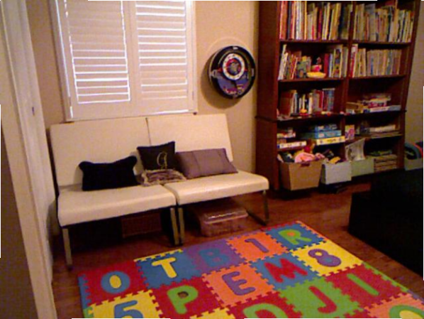
(a)

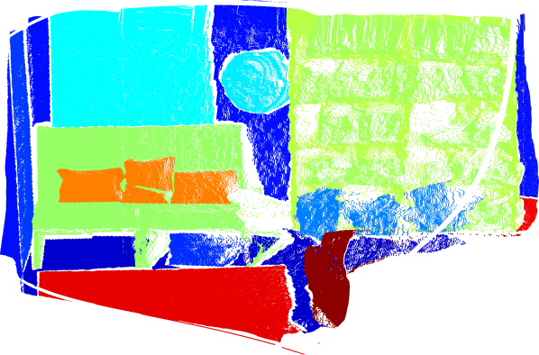
(b)

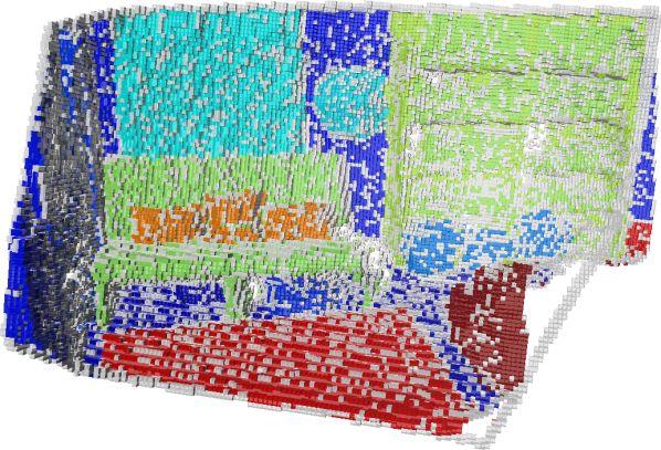
(c)

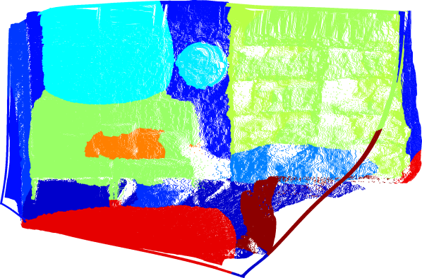
(d)

Figure 1: The figure shows examples of the GPSM (bottom right) and SOM (bottom left) using NYU Depth V2 dataset. The point cloud with ground truth semantic labels is shown in the top right. The maps are built by uniformly down-sampling the original point cloud to one-third. The GP map can infer the missing labels and deal with sparse measurements. The query points are the same as original points in the top right.

In this paper, we formulate the semantic mapping as a multi-class classification problem and use raw pixelated semantic measurements (class labels) to generalize the traditional occupied and unoccupied class assignment. The proposed Gaussian Processes Semantic Map (GPSM) is inherently continuous, and prediction can be made at any desired location. We use kernel methods in the form of GPs to systematically accept inputs with any dimensionality as well as heterogeneous bases such as spatial coordinates and colors. Figure 1 shows examples of Semantic OctoMap (SOM) and GPSM built using a single frame of NYU Depth V2 dataset [37]. In particular, this work has the following contributions:

1. The proposed technique infers the structural and semantic correlation from measurements rather than resorting to assumptions. Through learning the correlation in data, GPSM can infer missing labels and deal with sparse measurements.

2. GPSM is continuous, and queries can be made at any desired locations; therefore, the map can be inferred with any resolution.

3. GPSM is the extension of GPs occupancy maps, i.e. binary maps, to the multi-class semantic representation which provides rich maps for robotic planning tasks.

4. GPSM is agnostic to the input dimensions and can handle an arbitrary number of non-spatial dimensions .

Outline

In the following section, a review of the related work is given. The problem statement and preliminaries are discussed in Section III. The detailed formulation of the GP semantic mapping is presented in Section IV. The semantic OctoMap as an alternative map building technique is described in Section V. Section VI includes the time complexity analysis of both GP semantic map and semantic OctoMap. The Comparison of mapping results using a publicly available dataset is presented in Section VII; and finally, Section VIII concludes the paper and discusses possible extensions of this work.

Notation

In the present article probabilities and probability densities are not distinguished in general. Matrices are capitalized in bold, such as in $\boldsymbol{X}$, and vectors are in lower case bold type, such as in $\boldsymbol{x}$. Vectors are column-wise and $1\colon n$ means integers from $1$ to $n$. The Euclidean norm is shown by $\lVert\cdot\rVert$. $\lvert\boldsymbol{X}\rvert$ denotes the determinant of matrix $\boldsymbol{X}$. For the sake of compactness, random variables, such as $X$, and their realizations, $x$, are sometimes denoted interchangeably where it is evident from context. $x^{[i]}$ denotes a reference to the $i$-th element of the variable. An alphabet such as $\mathcal{X}$ denotes a set, and the cardinality of the set is denoted by $\lvert\mathcal{X}\rvert$. A subscript asterisk, such as in $\boldsymbol{x}_{*}$, indicates a reference to a test set quantity. The $n$-by-$n$ identity matrix is denoted by $\boldsymbol{I}_{n}$. We use $\mathrm{vec}(\boldsymbol{x},\boldsymbol{y})$ to construct a vector by stacking $\boldsymbol{x}$ and $\boldsymbol{y}$. The function notation is overloaded based on the output type and denoted by $k(\cdot)$, $\boldsymbol{k}(\cdot)$, and $\boldsymbol{K}(\cdot)$ where the outputs are scalar, vector, and matrix, respectively. Finally, $\mathbb{E}[\cdot]$ and $\mathbb{V}[\cdot]$ denote the expected value and variance of a random variable, respectively.

II Related Work

Early work in the context of robotic semantic mapping focused on room and building structure semantics, similar to topological mapping. Kuipers and Byun [27] create a network of distinctive places to map and explore large scale environments. Mozos et al. [35] assign labels to a 2D map of the indoor space corresponding to different parts of an indoor environment, such as room, corridor, and doorway through applying a classifier to the information collected by a range sensor. Then a Hidden Markov Model is used to encode transition probabilities to different labels, and thus using topological information. Pronobis et al. [41] extend that framework to include visual features, namely Scale-Invariant Feature Transform (SIFT) [31] and Composite Receptive Field Histograms (CRFH) [29]. Another interesting form of semantics for Simultaneous Localization And Mapping (SLAM) is object level classification. While room level semantics and topology are useful for navigation and exploration, object level semantics enable finer grained tasks such as robotic manipulation. Castle et al. [5] use a database of known planar objects to match SIFT features of a monocular video stream in an extended Kalman filter SLAM framework. Civera et al. [10] extend this approach to arbitrary three-dimensional (3D) geometries. Bao and Savarese [3] use an object detector in the structure from motion setup to jointly estimate camera parameters, 3D points, and object instances and poses. These approaches are developed to improve scene estimation by providing more geometric constraints. Conversely, Pillai and Leonard [40] use monocular SLAM to aggregate multiple views of a single object to provide more evidence to the object detector.

Dense 3D priors of objects have also been used for mapping and scene understanding. Kim et al. [24] learn models that are a collection of primitive 3D shapes; and show once a model based on primitives is learned, the object can quickly be recognized in an environment. Salas-Moreno et al. [43] align 3D mesh model priors of objects to the RGBD frame. The technique treats objects as landmarks and each alignment as a factor in the graphical SLAM framework. Choudhary et al. [9] also use objects as landmarks, but instead of having a dense 3D prior for every object, the objects are discovered via segmentation, and then their models are produced during the mapping process.

Beyond just object models, there has been work to produce 3D maps with dense semantic labels. Kundu et al. [28] jointly reconstruct the 3D scene and perform semantic segmentation. The technique uses a Conditional Random Field (CRF) to infer the semantic category and occupancy for each voxel jointly. Sengupta and Sturgess [44] also look at semantic segmentation and reconstruction of the 3D scene; the technique uses stereo images, estimated camera pose, and a CRF defined over voxels and supervoxels of the octree to infer the semantic octree representation of the 3D scene. Vineet et al. [53] propose an incremental dense stereo reconstruction and semantic segmentation technique. To address the challenge of dealing with moving objects, Kochanov et al. [26] present a method to incorporate temporal updates into the map using scene flow measurements.

In this paper, we propose the GP semantic map to infer the structural and semantic representation of the scene concurrently. Our approach fundamentally differs from the above-mentioned techniques as it does not discretize the map and is continuous. While in the present work, we focus on the problem formulation and 3D reconstruction of a single RGBD scan, the proposed framework can be used for the 3D scene reconstruction using map fusion algorithms [14]. Furthermore, the techniques mentioned earlier ignore pose estimation uncertainty in the map building process; however, our framework is systematically capable of accepting uncertain inputs [16].

III Problem Statement and Preliminaries

The objective is formulate and solve the mapping process in a fully probabilistic framework. Since the environment representation we consider here is dense and measurements can be sparse due to the limited sensor field of view and range, a simple inference on individual voxels can lead to a poor mapping performance. Therefore, we devise a joint inference scheme based on GPs by assuming map points are normally distributed. In particular, the following assumption are made.

Assumption 1 (Static map representation).

The environment is static.

Assumption 2 (Gaussian map points).

Any sampled point from the semantic map representation of the environment is a random variable whose distribution is Gaussian.

From Assumption 2, and placing a joint distribution over map points, the mapping process by definition can be modeled as a GP.

Definition 1 (Gaussian process [42]).

A Gaussian process is a collection of random variables, any finite number of which have a joint Gaussian distribution.

Problem 1 (Gaussian processes semantic map).

Given a point cloud measurement that is (possibly partially) assigned with noisy semantic class labels, infer a semantic map representation of the point cloud as a Gaussian process.

III-A Gaussian Processes Regression

GPs are nonparametric Bayesian regression techniques that employ statistical inference to learn dependencies between points in a data set [42]. The joint distribution of the observed target values, $\boldsymbol{y}$, and the function values (the latent variable), $\boldsymbol{f}_{*}$, at the query points can be written as

$$\begin{bmatrix}\boldsymbol{y}\\ \boldsymbol{f}_{*}\end{bmatrix}\sim\mathcal{N}(\boldsymbol{0},\begin{bmatrix}\boldsymbol{K}(\boldsymbol{X},\boldsymbol{X})+\sigma_{n}^{2}\boldsymbol{I}_{n}&\boldsymbol{K}(\boldsymbol{X},\boldsymbol{X}_{*})\\ \boldsymbol{K}(\boldsymbol{X}_{*},\boldsymbol{X})&\boldsymbol{K}(\boldsymbol{X}_{*},\boldsymbol{X}_{*})\end{bmatrix})$$ (1)

where $\boldsymbol{X}$ is the $d\times n$ design matrix of aggregated input vectors $\boldsymbol{x}$, $\boldsymbol{X}_{*}$ is a $d\times n_{*}$ query points matrix, $\boldsymbol{K}(\cdot,\cdot)$ is the GP covariance matrix, and $\sigma_{n}^{2}$ is the variance of the observation noise which is assumed to have an independent and identically distributed (i.i.d.) Gaussian distribution. The predictive conditional distribution for a single query point $f_{*}|\boldsymbol{X},\boldsymbol{y},\boldsymbol{x}_{*}\sim\mathcal{N}(\mathbb{E}[f_{*}],\mathbb{V}[f_{*}])$ can be derived as

$$\mathbb{E}[f_{*}]=\boldsymbol{k}(\boldsymbol{X},\boldsymbol{x}_{*})^{T}[\boldsymbol{K}(\boldsymbol{X},\boldsymbol{X})+\sigma_{n}^{2}\boldsymbol{I}_{n}]^{-1}\boldsymbol{y}$$ (2)

$$\mathbb{V}[f_{*}]= k(\boldsymbol{x}_{*},\boldsymbol{x}_{*})$$

$$-\boldsymbol{k}(\boldsymbol{X},\boldsymbol{x}_{*})^{T}[\boldsymbol{K}(\boldsymbol{X},\boldsymbol{X})+\sigma_{n}^{2}\boldsymbol{I}_{n}]^{-1}\boldsymbol{k}(\boldsymbol{X},\boldsymbol{x}_{*})$$ (3)

III-B Gaussian Processes Classification

Supervised classification is the problem of learning input-output mappings from a training dataset for discrete outputs (class labels). In binary GP Classification (GPC), we define class labels as $y\in\{\pm 1\}$. In GPC, the inference is performed in two steps. First computing the predictive distribution of the latent variable corresponding to a query case, $f_{*}|\boldsymbol{X},\boldsymbol{y},\boldsymbol{x}_{*}\sim\mathcal{N}(\mathbb{E}[f_{*}],\mathbb{V}[f_{*}])$, and then a probabilistic prediction, $p(y_{*}=+1|\boldsymbol{X},\boldsymbol{y},\boldsymbol{x}_{*})$, using a sigmoid function, $\sigma(\cdot)$, that assigns class labels with a probability that increases monotonically with the latent. The non-Gaussian likelihood and the choice of the sigmoid function can make the inference analytically intractable. Hence, approximate inference techniques are required.

III-C Model Selection

In GPs, one can learn free parameters of mean, covariance, and likelihood functions (hyperparameters) through optimizing a cost function. Practically, The hyperparameters, $\boldsymbol{\theta}$, can be computed by minimization of the negative log of the marginal likelihood (NLML) function.

$$\log p(\boldsymbol{y}|\boldsymbol{X},\boldsymbol{\theta}) =-\frac{1}{2}\boldsymbol{y}^{T}(\boldsymbol{K}(\boldsymbol{X},\boldsymbol{X})+\sigma_{n}^{2}\boldsymbol{I}_{n})^{-1}\boldsymbol{y}$$

$$-\frac{1}{2}\log\arrowvert K(\boldsymbol{X},\boldsymbol{X})+\sigma_{n}^{2}\boldsymbol{I}_{n}\arrowvert-\frac{n}{2}\log 2\pi\$$ (4)

In (III-C), the first term $-\frac{1}{2}\boldsymbol{y}^{T}(\boldsymbol{K}(\boldsymbol{X},\boldsymbol{X})+\sigma_{n}^{2}\boldsymbol{I}_{n})^{-1}\boldsymbol{y}$ corresponds to data-fit, the second term $\frac{1}{2}\log\ \arrowvert K(\boldsymbol{X},\boldsymbol{X})+\sigma_{n}^{2}\boldsymbol{I}_{n}\arrowvert$ penalizes the model complexity, and the last term is a constant.

Remark 1.

Note that the selection of NLML function for the optimization problem is entirely optional. However due to the marginalization property of the multivariate normal distribution, the latent variable $\boldsymbol{f}_{*}$ can be conveniently marginalized.

Remark 2.

Generally speaking, building maps using GPs can handle sparse sensor observations and consequently sparse training data. However, in practice, the kernel function describes the correlation between training points. A smooth kernel such as the squared exponential can cover a larger area with fewer training points, and a rough kernel such as Matérn ($\nu=1/2$) can only cover the vicinity of sparse training points, see Rasmussen and Williams [42, Figure 4.1]. Therefore, model selection is crucial to fully exploit capabilities of GPs. Furthermore, hyperparameters have a significant effect on the shape of the map.

The GPC model implemented in this work uses a constant mean function, Matérn ($\nu=5/2$) covariance function [48] with automatic relevance determination [38], the error function likelihood (probit regression), and Laplace technique for approximate inference and is done using the open source GP library in [42]. It is argued in Stein [48] that Matérn covariance functions are more suitable for modeling physical processes.

III-D Large-scale Inference

The main bottleneck in GP regression is computation of the term $[\boldsymbol{K}(\boldsymbol{X},\boldsymbol{X})+\sigma_{n}^{2}\boldsymbol{I}_{n}]^{-1}$ where the covariance matrix of training data has to be inverted. This limitation reveals itself more when one tries to use a large number of training data. In general, the number of measurements in a point cloud exceeds a few hundred and can be up to several hundred thousands. In such cases, approximate inference techniques such as Laplace, expectation propagation [33], or variational Bayes [20] can become time-consuming. The Fully Independent Training Conditional (FITC) [46, 36] method is based on a low-rank plus diagonal approximation to the exact covariance matrix and is computationally more attractive while it preserves the desirable properties of the full GP [46]. In particular, FITC uses a set of inducing points to shift the computational cost on the cross-covariances computation between training, test, and inducing points.

IV Gaussian Processes Semantic Map

In this section, we formulate the GP semantic map to solve Problem 1. While the formulation we present here is general, for the classification purpose, we use a binary GPC as the base classifier for each class and one-vs.-rest approach to building a multi-class classifier. However, we acknowledge that the multi-class Laplace approximation in Rasmussen and Williams [42, Section 3.5] is an interesting approach to building a true probabilistic multi-class classifier.

Let $\mathcal{M}$ be the set of possible semantic maps. We consider the map of the environment as an $n_{m}$-tuple random variable $(M^{[1]},\dots,M^{[n_{m}]})$ whose elements are described by a normal distribution $m^{[i]}\sim\mathcal{N}(\mu^{[i]},v^{[i]})$, $i\in\{1\colon n_{m}\}$. Let $\mathcal{X}\subset\mathbb{R}^{3}$ be the set of spatial coordinates to build a map on, and $\mathcal{C}=\{c^{[j]}\}_{j=1}^{n_{c}}$ be the set of semantic class labels. Let $\mathcal{Z}\subset\mathcal{X}\times\mathcal{C}$ be the set of possible measurements. The observation consists of an $n_{z}$-tuple random variable $(Z^{[1]},\dots,Z^{[n_{z}]})$ whose elements can take values $\boldsymbol{z}^{[k]}\in\mathcal{Z}$, $k\in\{1\colon n_{z}\}$ where $\boldsymbol{z}^{[k]}=(\boldsymbol{x}^{[k]},y^{[k]})$, $\boldsymbol{x}^{[k]}\in\mathcal{X}$, and $y^{[k]}\in\mathcal{C}$.

We define a training set $\mathcal{D}=\{(\boldsymbol{x}^{[i]},y^{[i]})\}_{i=1}^{n_{t}}$ and the target vector $\boldsymbol{y}=\mathrm{vec}(y^{[1]},\dots,y^{[n_{t}]})$ where $\mathcal{D}\subseteq\mathcal{Z}$, and $n_{t}\leq n_{z}$ is the number of training points. Given observations $Z=\boldsymbol{z}$, we wish to estimate $p(M=m\mid Z=\boldsymbol{z})$. The map can be inferred as a Gaussian process by defining the process as the function $y:\mathcal{Z}\rightarrow\mathcal{M}$, therefore

$$y(\boldsymbol{x})\sim\mathcal{GP}(f_{m}(\boldsymbol{x}),k(\boldsymbol{x},\boldsymbol{x}^{\prime}))$$ (5)

It is often the case that we set the mean function $f_{m}(\boldsymbol{x})$ as zero, unless it is mentioned explicitly that $f_{m}(\boldsymbol{x})\neq 0$. For a given query point in the map, $\boldsymbol{x}_{*}$, GP predicts a mean, $\mu$, and an associated variance, $v$. Thus, for any map point, we have $m^{[i]}=y(\boldsymbol{x}^{[i]}_{*})\sim\mathcal{N}(\mu^{[i]},v^{[i]})$.

Once the mean and variance of the latent $f_{*}$ are available, we predict the averaged predictive probability of the class $c^{[j]}$ as follow [42, Chapter 3].

$$p(c^{[j]}=+1|\mathcal{D},\boldsymbol{x}_{*})=\int\sigma(u)\mathcal{N}(u\mid\mathbb{E}[f_{*}],\mathbb{V}[f_{*}])du$$ (6)

Note that once the $n_{c}$ binary GPC are trained, and the prediction at query points (map points) are performed, we normalize the class probabilities to get $p(M=c^{[j]}|\boldsymbol{z})$ for the $j$-th semantic class. One straightforward way to assign hard labels to map points is to find the class with the maximum probability.

Remark 3.

The actual representation of the map depends on the distribution of query points. It is often the case to use uniformly distributed points. In general, query points can have any desired distributions. However, in this work, we use the original dense point cloud as the query points to facilitate comparison with the ground truth.

Example 1 (Two-dimensional Toy Example).

Figure 2 illustrates a two-dimensional toy example of GP multi-class classification that can be extended to the three-dimensional semantic mapping. The continuity and smoothness of the probabilistic inference are evident from the left plot, while the corresponding contour curves and the synthetic training points are shown in the right plot. The plots show the log probabilities.

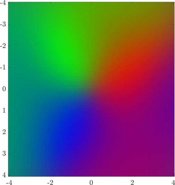
(a)

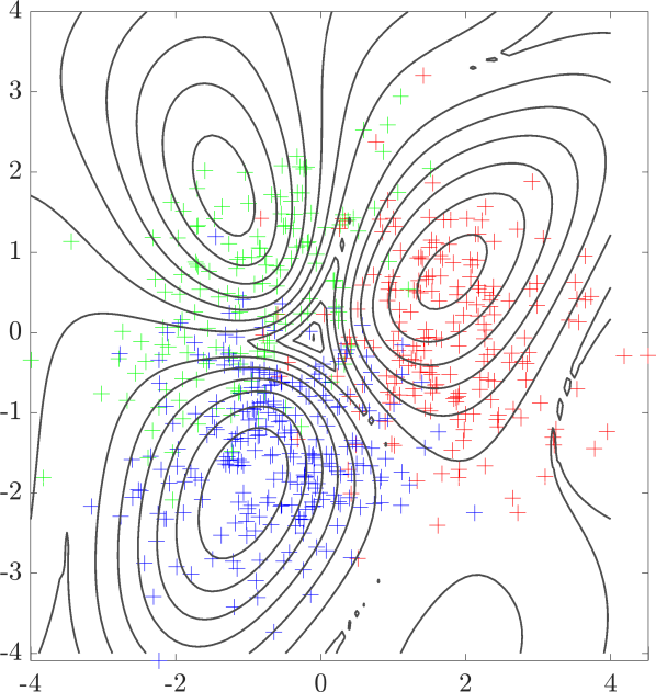
(b)

Figure 2: A two-dimensional toy example of GP multi-class classification using the synthetic dataset shown in the right plot. The prediction is continuous, and the class probabilities can be queries at any point in the plane as shown in the left plot. Furthermore, the contour curves can be seen as decision boundaries. The plots show the log probabilities.

V Semantic OctoMap

The OctoMap [19] is a popular robotic occupancy mapping tool which builds a discretized model of the 3D world using the octree data structure. The octree enables the multi-resolution map representation which has the advantage of being memory-efficient. In this section, we develop a simple extension of this technique to semantic OctoMap which will serve as the alternative approach in the presented evaluations in Section VII. In the basic OctoMap implementation, voxels only contain occupancy probability represented as log-odds. In the developed semantic OctoMap, in addition, voxels include semantic labeling and color information for visualization. The incorporation of the semantic knowledge into the OctoMap is also discussed in Sengupta and Sturgess [44].

Following the problem formulation in the previous section, given observations $Z=\boldsymbol{z}$, we wish to estimate $p(M=m\mid Z=\boldsymbol{z})$. The fundamental assumptions of this approach are as follows. First, the map posterior is approximated as the product of its marginals [50]:

$$p(M=m\mid Z=\boldsymbol{z})=\prod_{i=1}^{n_{m}}p(M=m^{[i]}\mid Z=\boldsymbol{z})$$ (7)

which indicates the distribution of each voxel is independent of the others. Second, we assume that for each voxel, the occupancy and semantic probabilities are independent. Based on these tow assumptions, we can process occupancy and semantic beliefs separately. We first use OctoMap library to compute the occupancy probability of each voxel. The principle is that voxels correspond to endpoints are updated as hits, while voxels along the ray between the sensor origin and the endpoint are updated as misses.

We follow the idea in Kochanov et al. [26] to define the semantic likelihood. The idea is to simply average the discrete semantic class labels that fall within a voxel. Let $\mathcal{L}^{[i]}$ be a multiset that contains semantic label observation, $l^{[i,j]}\in\mathcal{C}$, that are inside the $i$-th voxel. The likelihood function to update the semantic belief of the $j$-th class for the $i$-th voxel can be defined as follows.

$$p(c^{[j]}=+1\mid Z)=\frac{1}{\lvert\mathcal{L}^{[i]}\rvert}\sum_{s^{[k]}\in{\mathcal{L}^{[i]}}}p(s^{[k]}\mid Z)$$ (8)

For the visualization purpose, we only visualize the occupied voxels with their corresponding hard labels which are computed by finding the label with the maximum semantic probability. Figure 3 shows an example of the developed semantic OctoMap.

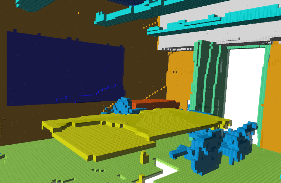
Figure 3: Semantic OctoMap built using the Stanford 2D-3D-Semantics Dataset [1], area 1, conference room 1. The semantic label observations are from the ground truth data. From the figure, the effect of discretization of the map and independent voxels inference are evident in the structural shape of the environment.

VI Computational Complexity Analysis

FITC uses inducing points (active set) to base the computations on cross-covariances between training, test, and inducing points; hence, the computational cost is dominated by the matrix multiplication and reduced from $\mathcal{O}(n_{t}^{3})$ to $\mathcal{O}(n_{t}n_{u}^{2})$ where $n_{u}$ is the number of inducing points and $n_{u}\ll n_{t}$. The computational complexity of the GP semantic map is dominated by FITC approximation and is the same.

The computational complexity of semantic OctoMap is determined by octree data access complexity, which is $\mathcal{O}(n_{d})=\mathcal{O}(\log{n_{n}})$, where $n_{n}$ is the total number of nodes and $n_{d}$ is the depth of the octree data structure. As semantics fusion process queries the corresponding voxel on an octree for each measured point in a scan, the computational complexity of this part is $\mathcal{O}(n_{p}\log{n_{n}})$, where $n_{p}$ is the number of points in the point cloud. It is worth mentioning that the maximum depth of octree is fixed in implementation; therefore, the practical computational complexity of the semantic fusion process is $\mathcal{O}(n_{p})$.

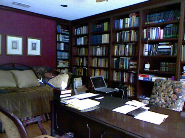
(a)

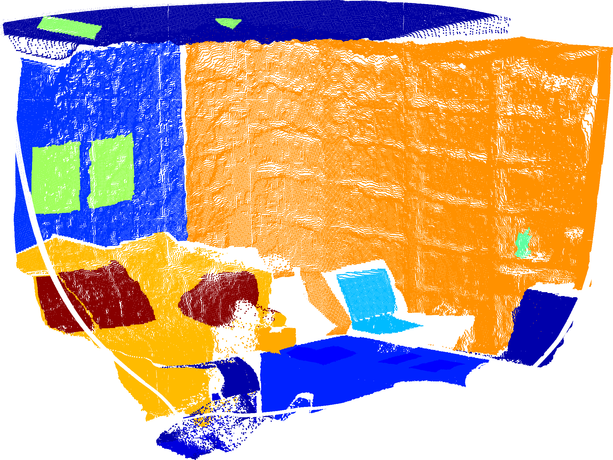
(b)

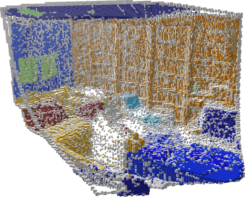
(c)

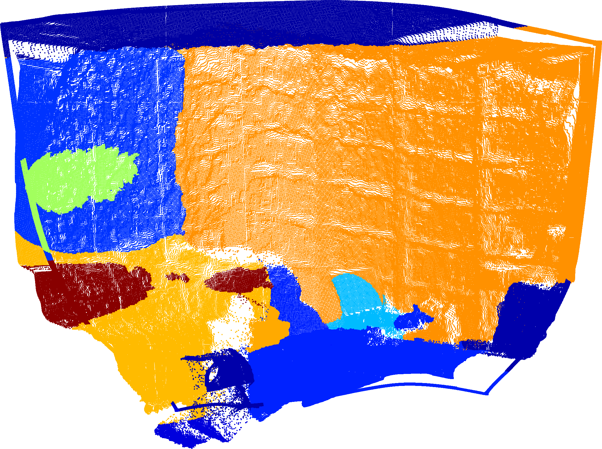
(d)

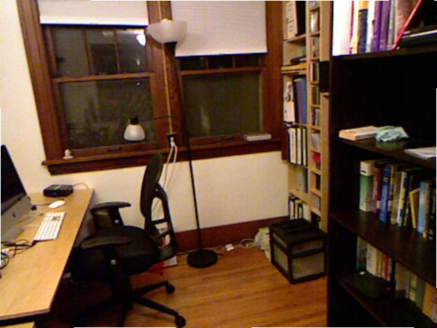
(e)

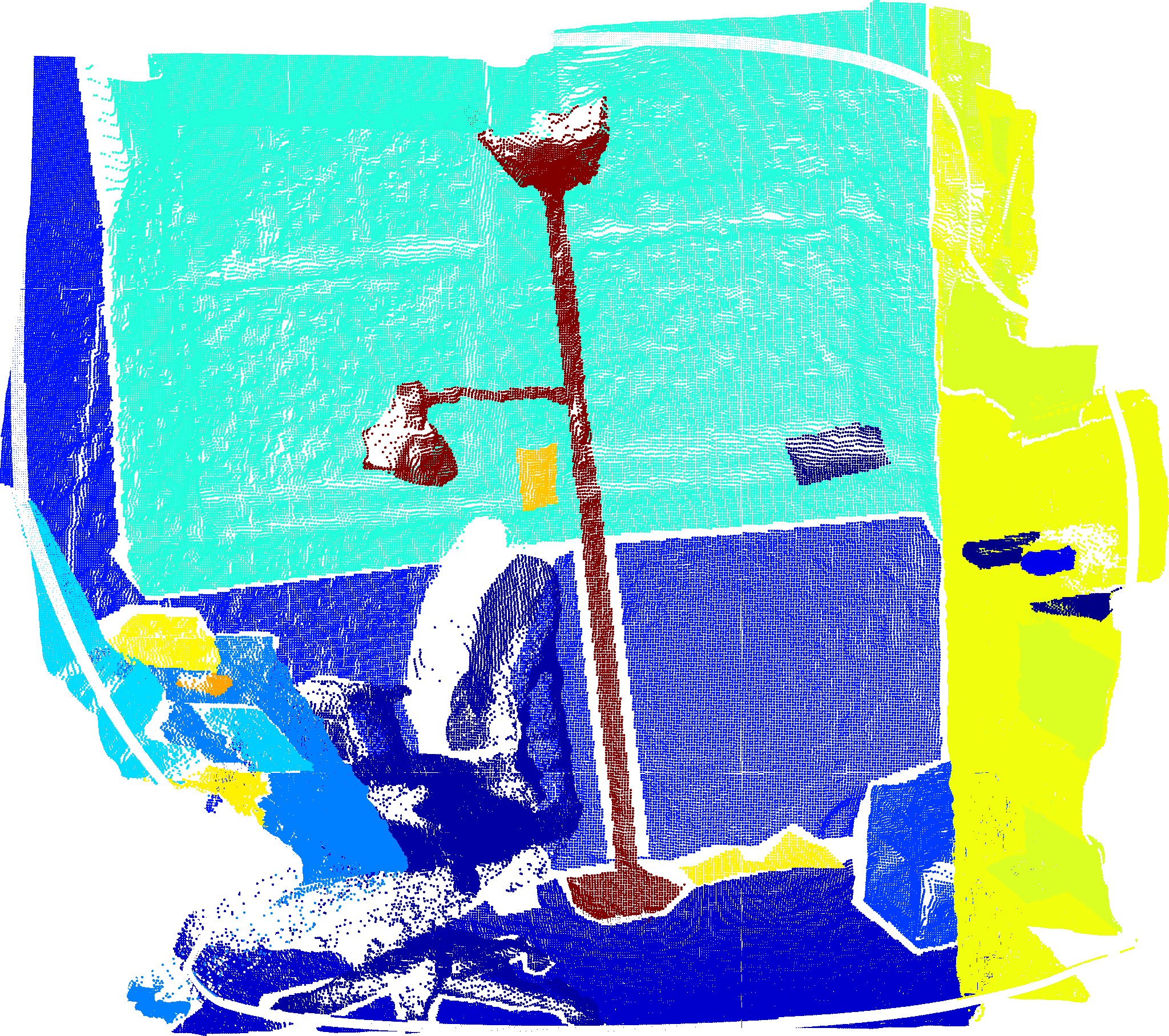
(f)

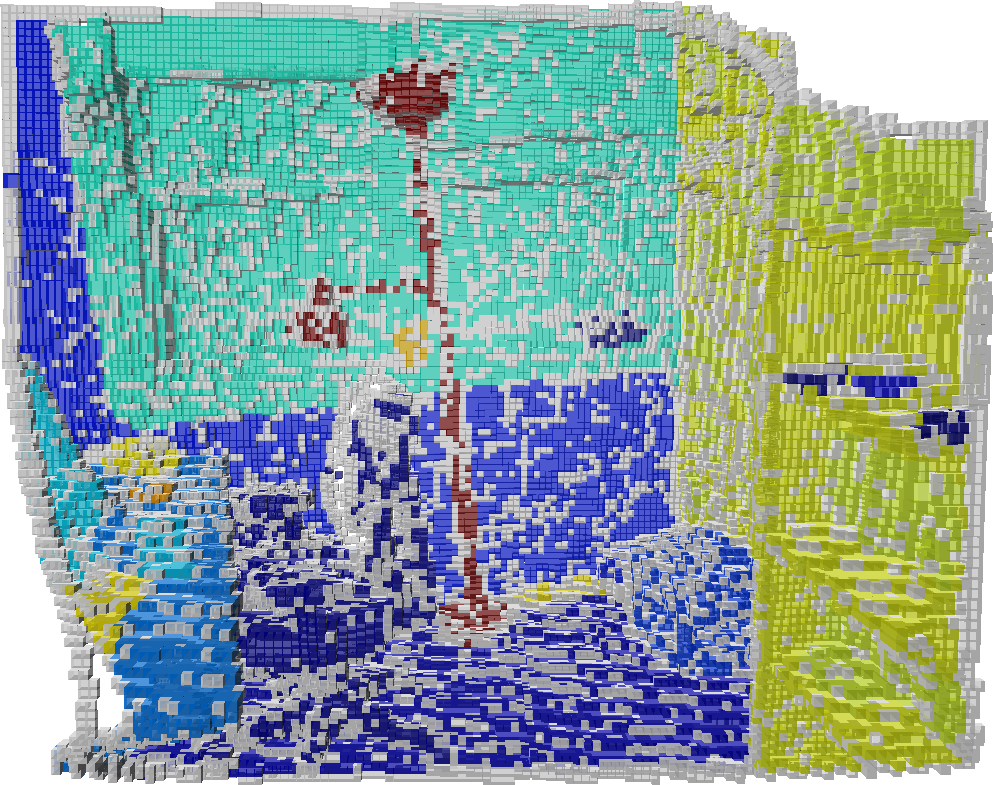
(g)

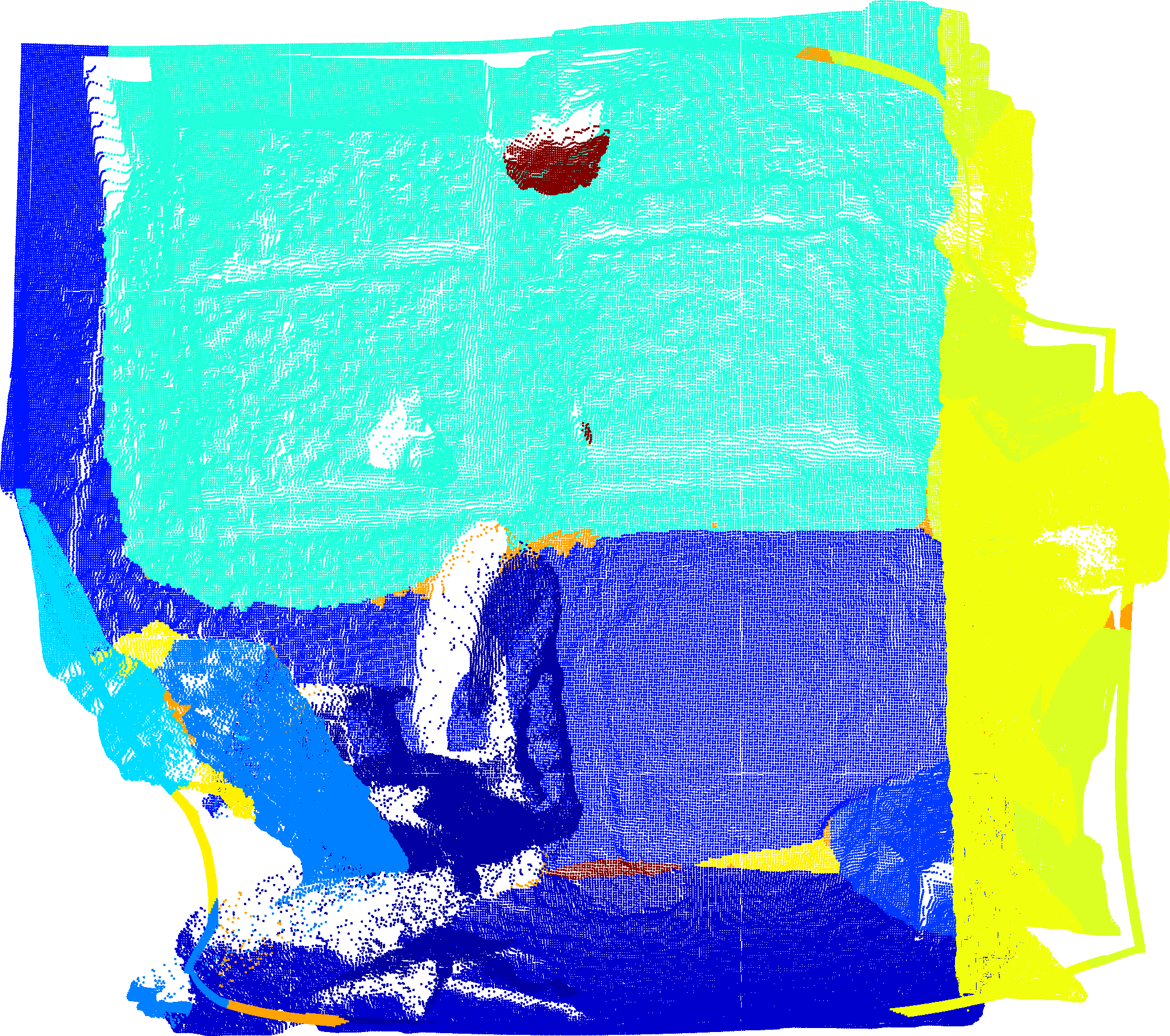
(h)

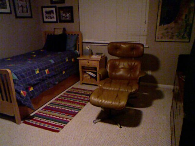
(i)

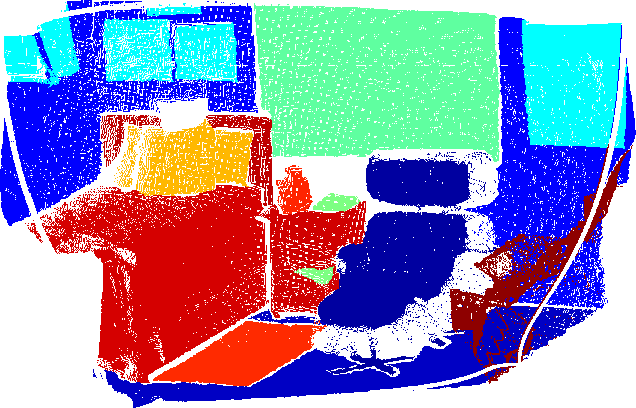
(j)

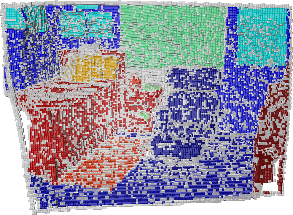
(k)

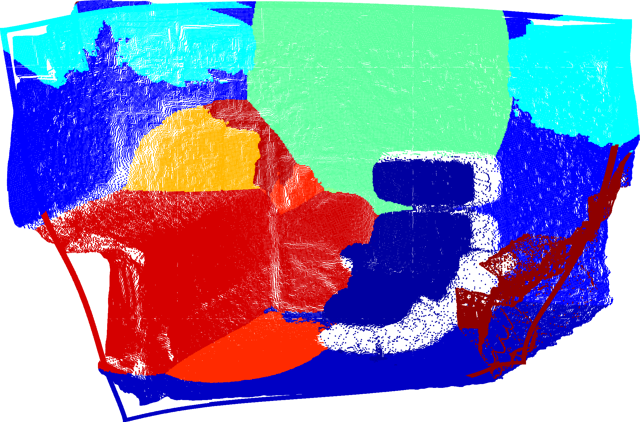
(l)

Figure 4: The figure shows GPSM and SOM results using sparse labeled point clouds. From left, each column respectively shows the RGB image, the point cloud with ground truth semantic labels before downsampling, the SOM, and the GPSM. The maps are built by uniformly down-sampling the original point cloud to one-third. The GP map can infer the missing labels and deal with sparse measurements through leaning the correlation between observations. For GPSM, the query points are the same as original points in the second column.

VII Results and Discussion

We now present mapping results using the proposed GP semantic map and the semantic OctoMap. We evaluate the proposed technique by comparing the mapping performance with that of the semantic OctoMap using NYU Depth V2 dataset [37]. The GPSM is implemented in MATLAB using the GPML library [42] and the SOM is implemented in C++ using by developing the original OctoMap implementation [19].

In the following, we explain the experimental setup and the performance criterion used for the comparison. We run two experiments; first, we study the effect of sparse measurements and missing labels by downsampling ground truth point clouds. Second, we use an image segmentation technique to label the entire point cloud to study the effect of misclassification (false positives) in observations.

VII-A Experimental Setup and Evaluation Criterion

The NYU Depth V2 dataset provides a large set of aligned RGB and depth images in indoor environments that are recorded by the Kinect sensor. The dataset also contains a subset of pixel-wise multi-class labeled images where there are unlabeled pixels in the annotated images for missing structures. We first convert RGBD scans to 3D point clouds with point-wise labels which serve as observation sets. Then we build the GPSM and the SOM. Note that, in this work, the map is referred to a local map built using a single scan (labeled point cloud). In the first experiment, point clouds are labeled using the ground truth semantic labels and downsampled by one-third to replicate sparse measurements and missing labels. In the second experiment, semantic labels are computed by the image segmentation technique SegNet [21]. The resolution of semantic OctoMap is set to $0.02\mathop{\mathrm{m}}$ for all results. The observation set contains about $300,000$ points. While the GP training points are a much smaller subset of the original observation set (typically less than $5000$ points), the query points are all points in the original point cloud.

The evaluations include the comparison of mapping performance using the Area Under the receiver operating characteristic Curve (AUC). The probability that the classifier ranks a randomly chosen positive instance higher than a randomly chosen negative instance can be understood using the AUC of the classifier; furthermore, the AUC is useful for domains with skewed class distribution and unequal classification error costs [12]. The AUC is originally a measure of the discriminability of a pair of classes. The extension of this method to the multi-class case is discussed in Hand and Till [18]. In order to maintain the performance measure insensitive to class distribution and error costs, following our one-vs.-rest multi-class classification approach, we calculate an AUC for each classifier (GP) and then take the average AUC as the overall performance measure. Thus, the total AUC can be computed as follows.

$$\mathrm{AUC}_{\mathrm{total}}=\frac{1}{\lvert\mathcal{C}\rvert}\sum_{j\in\mathcal{C}}\mathrm{AUC}^{[j]}$$ (9)

(a)

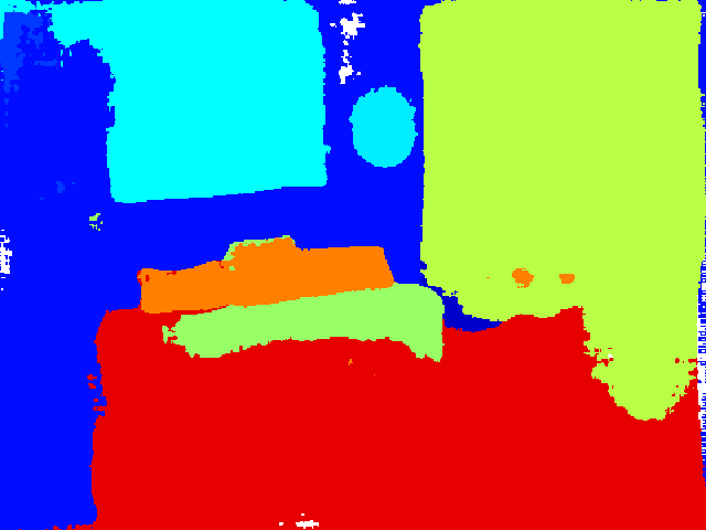
(b)

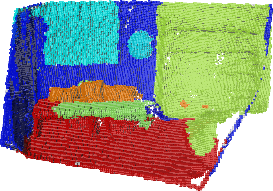
(c)

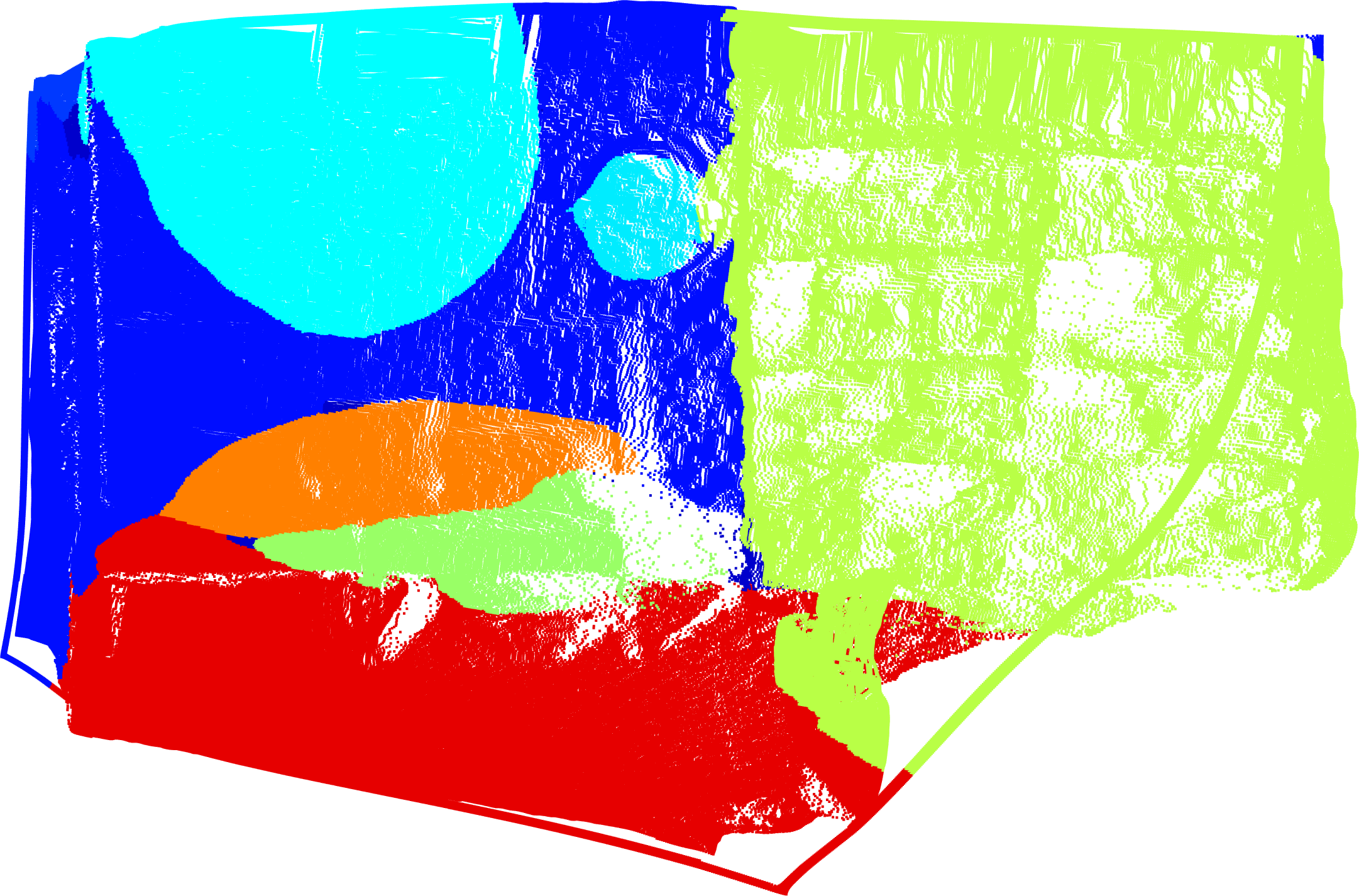
(d)

(e)

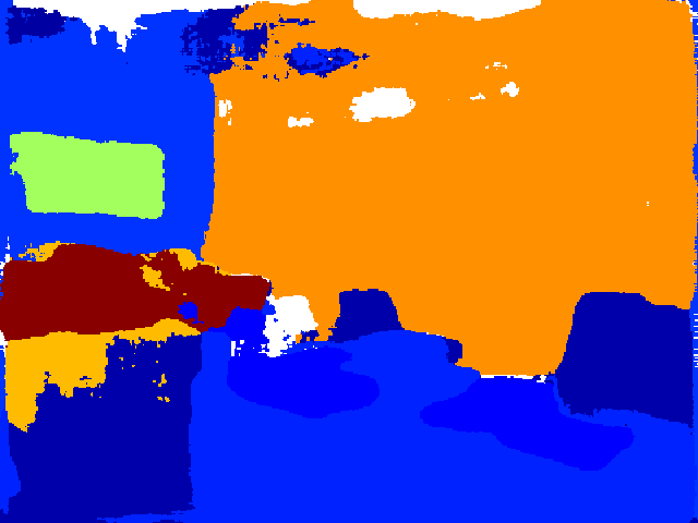
(f)

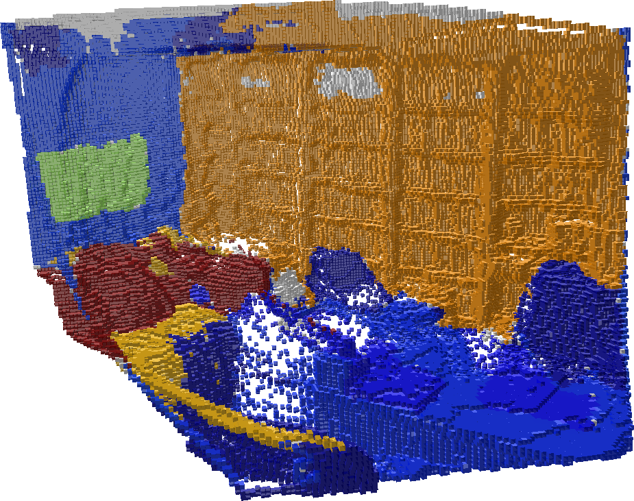
(g)

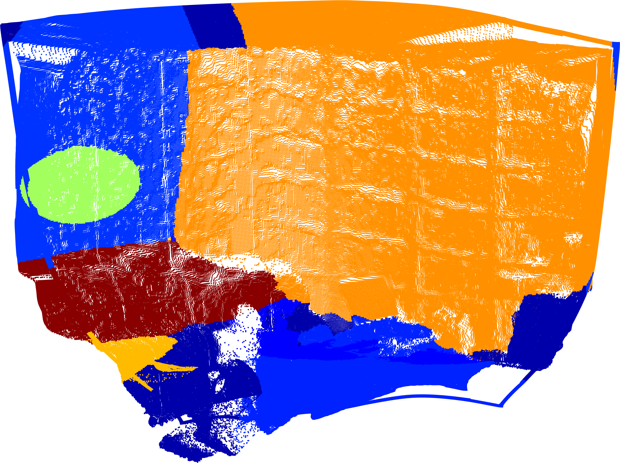
(h)

(i)

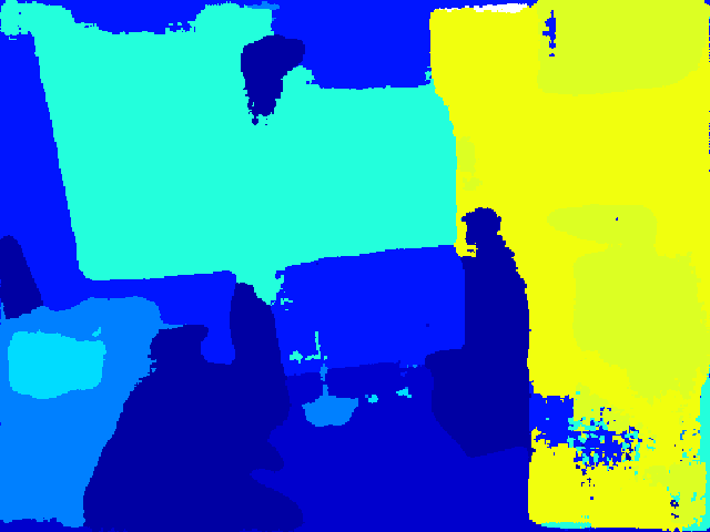
(j)

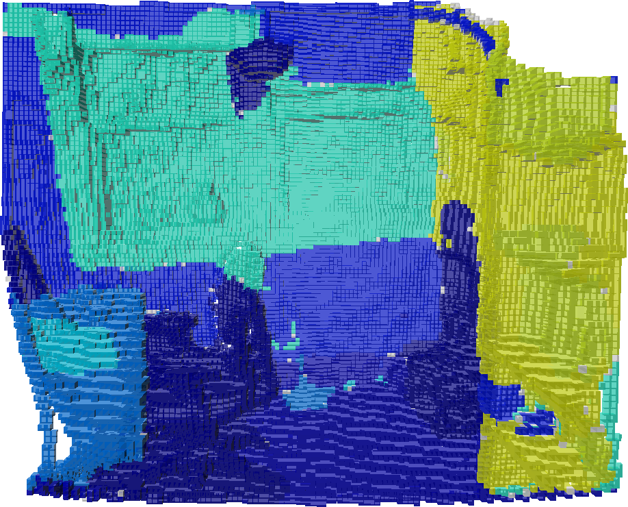
(k)

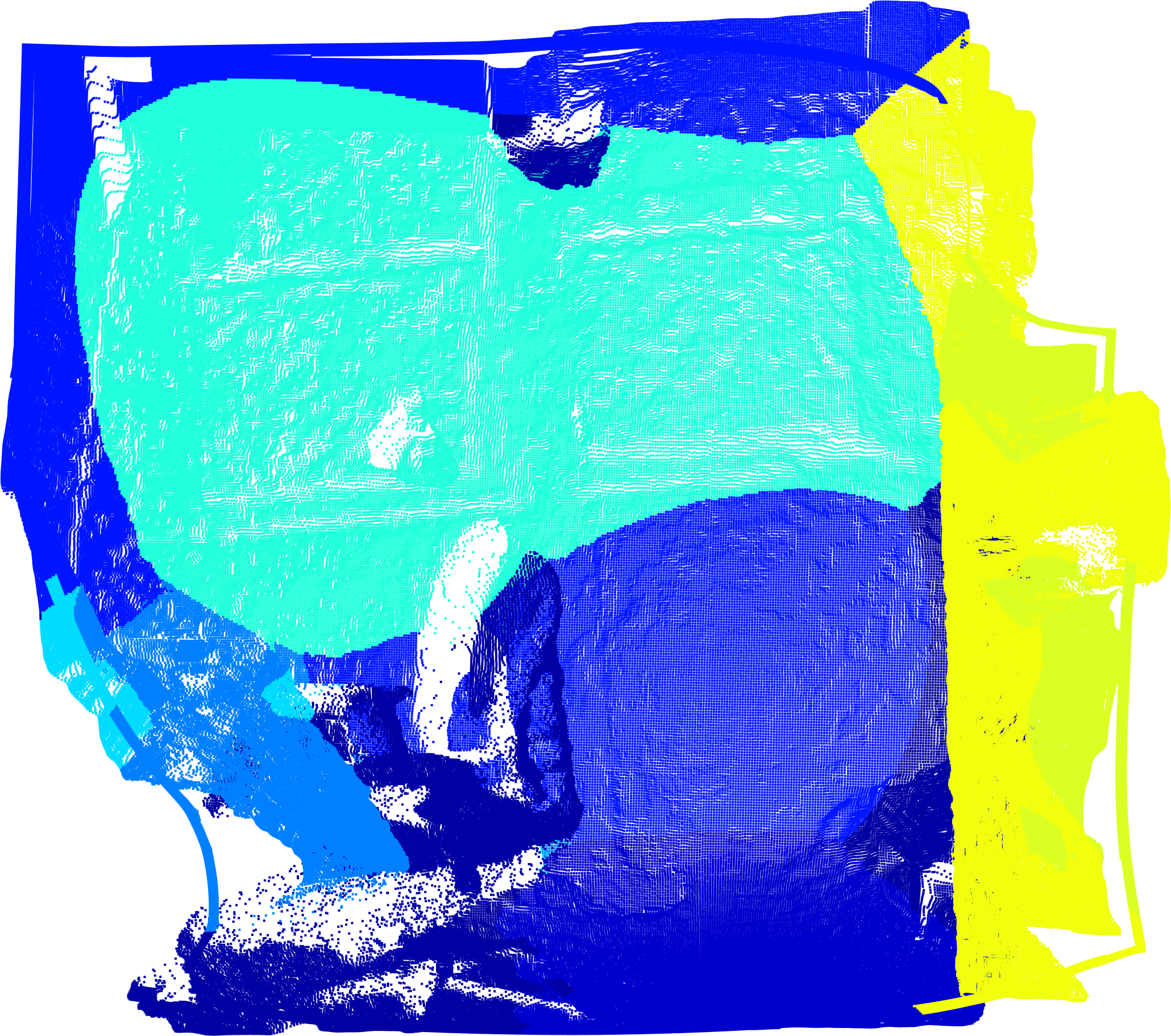
(l)

(m)

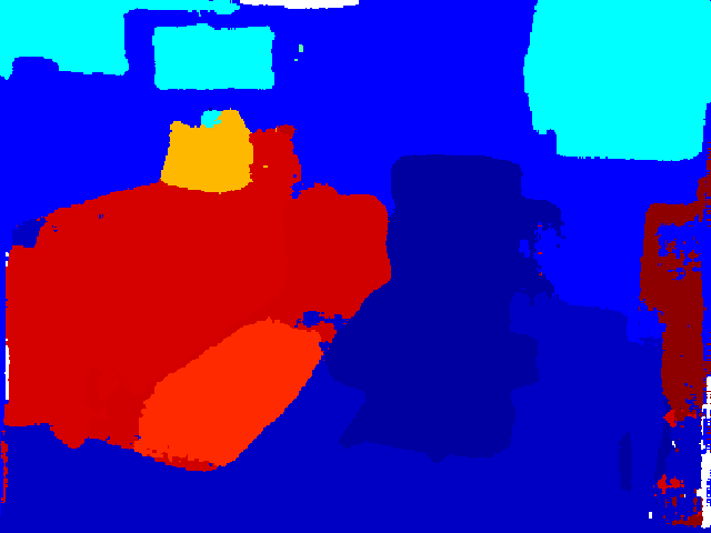
(n)

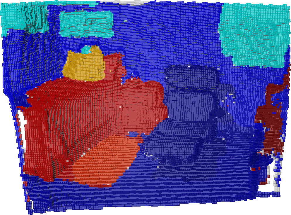
(o)

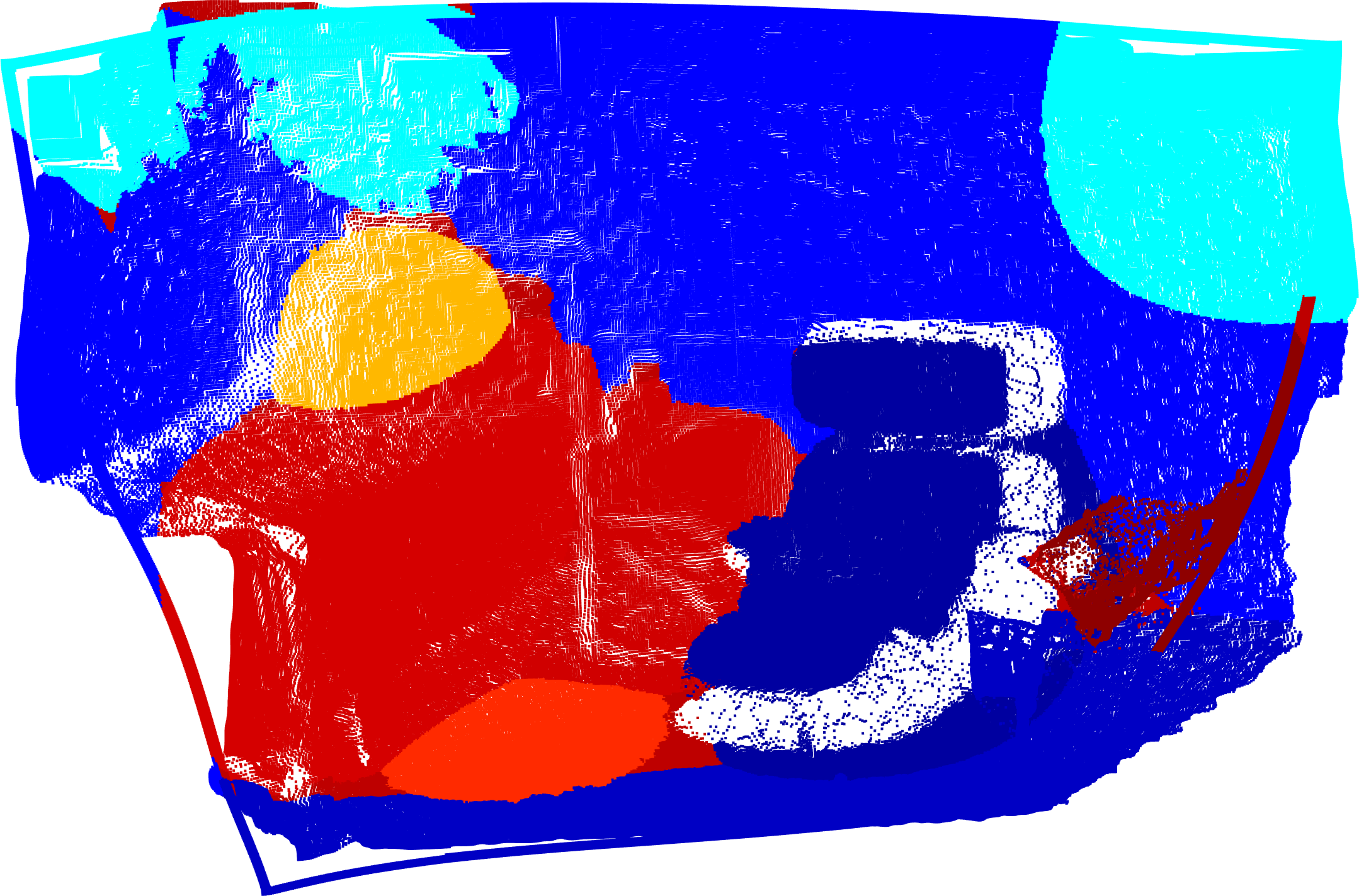
(p)

Figure 5: The results of mapping under noisy and misclassified labels. From left, each column respectively shows the RGB image, the image segmentation using SegNet, the SOM, and the GPSM results. The false positives in the image segmentation are directly transferred into the SOM results, while the GPSM uses the spatial distance between points to infer the class labels based on correlations between map points.

VII-B Sparse and Missing Measurements Effects

In the first experiment, we use four samples from the dataset for map building. The point clouds are labeled using the ground truth data. We uniformly downsample the labeled point clouds by one-third to replicate sparse measurements. As a result, since the number of labeled points is reduced, the point cloud contains many unlabeled points which makes the mapping process challenging. Figures 1 and 4 show the results of GPSM and SOM using the selected frames. Table I shows the quantitative comparison between GPSM and SOM.

TABLE I: The comparison of Gaussian processes semantic map and semantic OctoMap using the area under the receiver operating characteristic curve (AUC). The maps are built using downsampled point clouds from the NYU Depth V2 dataset [37] and the corresponding frame numbers are shown in the table.

Frame Number	GP Semantic Map	Semantic OctoMap
	$\mathrm{AUC}_{\mathrm{total}}$	$\mathrm{AUC}_{\mathrm{total}}$
NYU V2 - 282	0.9624	0.88525
NYU V2 - 374	0.9622	0.86251
NYU V2 - 555	0.9675	0.88648
NYU V2 - 965	0.9644	0.83569

From the result, the marginalization effect of the SOM on the map inference appears as many unlabeled voxels. Essentially, any voxel that does not contain any labeled points remains as unlabeled as there is no information available at that particular location. Intuitively, it is likely that neighboring locations share the same semantic class label and if any two points are spatially close, this chance can be even higher due to the present structural correlations in the environment. The lower mapping performance of the SOM, while dealing with sparse measurements, approves this claim.

The GP semantic map places a joint distribution on the observations and query points. This high-dimensional approach enables the method to infer the semantic class labels continuously. Furthermore, the available information in observations are captured in the GP covariance function which effectively models the correlation between map points. The GPSM is not limited to a fixed resolution and provides a probabilistic prediction and any desired location. The GPSM performs on all samples equally well with minor misclassified regions in each map. The maps are visualized using the class label with the maximum probability.

VII-C Mapping under Noisy and Misclassified Labels

In the second experiment, we use SegNet [21] to generate semantic labels. We first perform the RGB image segmentation and then assign each pixel’s label to its corresponding point in the point cloud. The mapping results are computed using the same four examples from the previous experiment, and the performance of each method is evaluated using the ground truth labeled point clouds in Figure 4. Figure 5 shows the results of the image segmentation (second column from left), the SOM (third column from left), and the GPSM (fourth column from left). Table II shows the quantitative comparison between GPSM and SOM. The challenge in this test is the presence of false positive labels in the observations and, as expected, both methods achieve lower mapping performance on the same set of data. Note that in this experiment the point clouds are not downsampled; however, the GP training set is a subset of observations as explained in the previous subsection.

The SOM directly uses the available points within a voxel to infer the voxel labels. Therefore, any misclassified label is transferred to the map. However, the GPSM infers the class labels based on the available correlations in the observation sets. Specifically, in the presented examples, the spatial correlations reduce the number of the misclassified points in the final map. For example, two adjacent pixels in the image space can have a similar label while their spatial distance can be large. Such cases are trivially handled in the GPSM framework since a large spatial distance implies insignificant correlation.

VII-D Discussion and Limitations

Since we seldom have sufficient information about a process, minimization of the NLML is a useful approach as it provides flexibility for model selection. However, the problem of minimizing NLML is an ill-posed problem and using maximum likelihood estimate we can often find a local minimum. Therefore, it is always possible that the solution suffers from overfitting, especially if the number of hyperparameters is large [42].

The common way for map representation in robotics is using a dense set of points with a particular distribution that is possibly suitable for navigation tasks. However, there is no restriction for any other desired representation such as approximate belief representations in Charrow et al. [6], that can be useful for other applications such as predictions. In fact, it is shown in Ghaffari Jadidi et al. [15] that by modeling the underlying process as GPs, one can perform information-theoretic planning using nonparametric information gain with possibility to handle the state estimate uncertainty [16].

In heteroscedastic processes, noise is state dependent. Heteroscedastic Gaussian process regression [17, 22] can be an alternative to model the structural correlation more accurately. However, to model the prediction uncertainty, they require a second GP in addition to the GP governing the noise-free output value. The computational cost is roughly twice that of the standard GP [25, 52]. To avoid increasing the computational time in the proposed mapping technique, we do not consider the heteroscedasticity in training data; however, applying these techniques to the problem at hand is an interesting direction to follow.

VIII Conclusion and Future Work

In this paper, we developed the Gaussian processes semantic map for 3D semantic map representations. We formulated the problem as a multi-class classification by defining the map spatial coordinates and semantic class labels as the input and output of the process, respectively. The proposed GP semantic map learns the structural and semantic correlation from measurements rather than resorting to assumptions, and exploits the spatial correlation (and possibly any additional non-spatial correlation) between map points for inference. In particular, the proposed map inference can infer missing labels and deal with sparse measurements, is continuous and queries can be made at any desired locations, and can deal with false positives better.

While, in this work, we only considered the spatial coordinates as the input, GPSM is agnostic to the input dimensions and can handle an arbitrary number of non-spatial dimensions. Future work includes extension of the proposed method to an incremental form and addition of other available dimensions such as color and intensity.

TABLE II: The comparison of Gaussian processes semantic map and semantic OctoMap using the area under the receiver operating characteristic curve (AUC). The maps are built using noisy image segmentation labels produced by SegNet. The figures for both methods are lower than the first experiment due to the presence of false positive labels in the observations.

Frame Number	GP Semantic Map	Semantic OctoMap
	$\mathrm{AUC}_{\mathrm{total}}$	$\mathrm{AUC}_{\mathrm{total}}$
NYU V2 - 282	0.7192	0.68402
NYU V2 - 374	0.7625	0.73552
NYU V2 - 555	0.7032	0.66881
NYU V2 - 965	0.8612	0.77456

References

- Armeni et al. [2017] I. Armeni, A. Sax, A. R. Zamir, and S. Savarese. Joint 2D-3D-Semantic Data for Indoor Scene Understanding. ArXiv e-prints, 2017.
- Badrinarayanan et al. [2015] Vijay Badrinarayanan, Alex Kendall, and Roberto Cipolla. SegNet: A deep convolutional encoder-decoder architecture for image segmentation. arXiv preprint arXiv:1511.00561, 2015.
- Bao and Savarese [2011] Sid Yingze Bao and Silvio Savarese. Semantic structure from motion. In Computer Vision and Pattern Recognition (CVPR), 2011 IEEE Conference on, pages 2025–2032. IEEE, 2011.
- Brostow et al. [2008] Gabriel Brostow, Jamie Shotton, Julien Fauqueur, and Roberto Cipolla. Segmentation and recognition using structure from motion point clouds. Computer Vision–ECCV 2008, pages 44–57, 2008.
- Castle et al. [2007] Robert O Castle, Darren J Gawley, Georg Klein, and David W Murray. Towards simultaneous recognition, localization and mapping for hand-held and wearable cameras. In Proc. IEEE Int. Conf. Robot Automat., pages 4102–4107, 2007.
- Charrow et al. [2014] Benjamin Charrow, Vijay Kumar, and Nathan Michael. Approximate representations for multi-robot control policies that maximize mutual information. Auton. Robot, 37(4):383–400, 2014.
- Charrow et al. [2015] Benjamin Charrow, Sikang Liu, Vijay Kumar, and Nathan Michael. Information-theoretic mapping using Cauchy-Schwarz quadratic mutual information. In Proc. IEEE Int. Conf. Robot Automat., pages 4791–4798. IEEE, 2015.
- Chen et al. [2016] Liang-Chieh Chen, George Papandreou, Iasonas Kokkinos, Kevin Murphy, and Alan L Yuille. Deeplab: Semantic image segmentation with deep convolutional nets, atrous convolution, and fully connected CRFs. arXiv preprint arXiv:1606.00915, 2016.
- Choudhary et al. [2014] Siddharth Choudhary, Alexander JB Trevor, Henrik I Christensen, and Frank Dellaert. SLAM with object discovery, modeling and mapping. In Proc. IEEE/RSJ Int. Conf. Intell. Robots Syst., pages 1018–1025, 2014.
- Civera et al. [2011] Javier Civera, Dorian Gálvez-López, Luis Riazuelo, Juan D Tardós, and JMM Montiel. Towards semantic SLAM using a monocular camera. In Proc. IEEE/RSJ Int. Conf. Intell. Robots Syst., pages 1277–1284, 2011.
- Elfes [1987] Alberto Elfes. Sonar-based real-world mapping and navigation. Robotics and Automation, IEEE Journal of, 3(3):249–265, 1987.
- Fawcett [2006] Tom Fawcett. An introduction to ROC analysis. Pattern recognition letters, 27(8):861–874, 2006.
- Ghaffari Jadidi et al. [2014] Maani Ghaffari Jadidi, Jaime Valls Miro, Rafael Valencia, and Juan Andrade-Cetto. Exploration on continuous Gaussian process frontier maps. In Proc. IEEE Int. Conf. Robot Automat., pages 6077–6082, 2014.
- Ghaffari Jadidi et al. [2017a] Maani Ghaffari Jadidi, Jaime Valls Miro, and Gamini Dissanayake. Gaussian process autonomous mapping and exploration for range sensing mobile robots. arXiv, 2017a. URL http://arxiv.org/abs/1605.00335.
- Ghaffari Jadidi et al. [2017b] Maani Ghaffari Jadidi, Jaime Valls Miro, and Gamini Dissanayake. Sampling-based incremental information gathering with applications to robotic exploration and environmental monitoring. arXiv, 2017b. URL http://arxiv.org/abs/1607.01883.
- Ghaffari Jadidi et al. [2017c] Maani Ghaffari Jadidi, Jaime Valls Miro, and Gamini Dissanayake. Warped Gaussian processes occupancy mapping with uncertain inputs. IEEE Robotics and Automation Letters, 2(2):680 – 687, 2017c.
- Goldberg et al. [1998] Paul W Goldberg, Christopher KI Williams, and Christopher M Bishop. Regression with input-dependent noise: A Gaussian process treatment. In NIPS, pages 493–499. 1998.
- Hand and Till [2001] David J Hand and Robert J Till. A simple generalisation of the area under the ROC curve for multiple class classification problems. Machine learning, 45(2):171–186, 2001.
- Hornung et al. [2013] Armin Hornung, Kai M Wurm, Maren Bennewitz, Cyrill Stachniss, and Wolfram Burgard. OctoMap: An efficient probabilistic 3d mapping framework based on octrees. Autonomous Robots, 34(3):189–206, 2013.
- Jordan et al. [1999] Michael I Jordan, Zoubin Ghahramani, Tommi S Jaakkola, and Lawrence K Saul. An introduction to variational methods for graphical models. Machine learning, 37(2):183–233, 1999.
- Kendall et al. [2015] Alex Kendall, Vijay Badrinarayanan, , and Roberto Cipolla. Bayesian SegNet: Model uncertainty in deep convolutional encoder-decoder architectures for scene understanding. arXiv preprint arXiv:1511.02680, 2015.
- Kersting et al. [2007] Kristian Kersting, Christian Plagemann, Patrick Pfaff, and Wolfram Burgard. Most likely heteroscedastic Gaussian process regression. In Proc. Int. Conf. Machine learning, pages 393–400. ACM, 2007.
- Kim and Kim [2013] Soohwan Kim and Jonghyuk Kim. Occupancy mapping and surface reconstruction using local Gaussian processes with Kinect sensors. IEEE Transactions on Cybernetics, 43(5):1335–1346, 2013.
- Kim et al. [2012] Young Min Kim, Niloy J Mitra, Dong-Ming Yan, and Leonidas Guibas. Acquiring 3D indoor environments with variability and repetition. ACM Transactions on Graphics (TOG), 31(6):138, 2012.
- Ko and Fox [2009] Jonathan Ko and Dieter Fox. GP-BayesFilters: Bayesian filtering using Gaussian process prediction and observation models. Auton. Robot, 27(1):75–90, 2009.
- Kochanov et al. [2016] Deyvid Kochanov, Aljoša Ošep, Jörg Stückler, and Bastian Leibe. Scene flow propagation for semantic mapping and object discovery in dynamic street scenes. In Proc. IEEE/RSJ Int. Conf. Intell. Robots Syst., pages 1785–1792, 2016.
- Kuipers and Byun [1991] Benjamin Kuipers and Yung-Tai Byun. A robot exploration and mapping strategy based on a semantic hierarchy of spatial representations. Robot. Auton. Syst., 8(1):47–63, 1991.
- Kundu et al. [2014] Abhijit Kundu, Yin Li, Frank Dellaert, Fuxin Li, and James M Rehg. Joint semantic segmentation and 3D reconstruction from monocular video. In European Conf. on Computer Vision, pages 703–718. Springer, 2014.
- Linde and Lindeberg [2004] Oskar Linde and Tony Lindeberg. Object recognition using composed receptive field histograms of higher dimensionality. In Proc. Int. Conf. Pattern Recognition, volume 2, pages 1–6. IEEE, 2004.
- Long et al. [2015] Jonathan Long, Evan Shelhamer, and Trevor Darrell. Fully convolutional networks for semantic segmentation. In Proceedings of the IEEE Conf. on Computer Vision and Pattern Recognition, pages 3431–3440, 2015.
- Lowe [2004] David G Lowe. Distinctive image features from scale-invariant keypoints. Int. journal of computer vision, 60(2):91–110, 2004.
- Merali and Barfoot [2014] Rehman S Merali and Timothy D Barfoot. Optimizing online occupancy grid mapping to capture the residual uncertainty. In Proc. IEEE Int. Conf. Robot Automat., pages 6070–6076. IEEE, 2014.
- Minka [2001] Thomas P Minka. A family of algorithms for approximate Bayesian inference. PhD thesis, Massachusetts Institute of Technology, 2001.
- Moravec and Elfes [1985] Hans P Moravec and Alberto Elfes. High resolution maps from wide angle sonar. In Proc. IEEE Int. Conf. Robot Automat., volume 2, pages 116–121. IEEE, 1985.
- Mozos et al. [2007] Oscar Martinez Mozos, Rudolph Triebel, Patric Jensfelt, Axel Rottmann, and Wolfram Burgard. Supervised semantic labeling of places using information extracted from sensor data. Robot. Auton. Syst., 55(5):391–402, 2007.
- Naish-Guzman and Holden [2007] Andrew Naish-Guzman and Sean B Holden. The generalized FITC approximation. In NIPS, pages 1057–1064, 2007.
- Nathan Silberman and Fergus [2012] Pushmeet Kohli Nathan Silberman, Derek Hoiem and Rob Fergus. Indoor segmentation and support inference from RGBD images. In ECCV, 2012.
- Neal [1996] Radford M Neal. Bayesian learning for neural networks, volume 118. Springer New York, 1996.
- Noh et al. [2015] Hyeonwoo Noh, Seunghoon Hong, and Bohyung Han. Learning deconvolution network for semantic segmentation. In Proceedings of the IEEE Int. Conf. on Computer Vision, pages 1520–1528, 2015.
- Pillai and Leonard [2015] Sudeep Pillai and John Leonard. Monocular SLAM supported object recognition. In Robotics: Science and Systems, Rome, Italy, July 2015.
- Pronobis et al. [2010] Andrzej Pronobis, O Martinez Mozos, Barbara Caputo, and Patric Jensfelt. Multi-modal semantic place classification. The Int. J. Robot. Res., 29(2-3):298–320, 2010.
- Rasmussen and Williams [2006] C.E. Rasmussen and C.K.I. Williams. Gaussian processes for machine learning, volume 1. MIT press, 2006.
- Salas-Moreno et al. [2013] Renato F Salas-Moreno, Richard A Newcombe, Hauke Strasdat, Paul HJ Kelly, and Andrew J Davison. SLAM++: Simultaneous localisation and mapping at the level of objects. In Proc. IEEE Conf. on Computer Vision and Pattern Recognition, pages 1352–1359, 2013.
- Sengupta and Sturgess [2015] Sunando Sengupta and Paul Sturgess. Semantic octree: Unifying recognition, reconstruction and representation via an octree constrained higher order MRF. In Proc. IEEE Int. Conf. Robot Automat., pages 1874–1879, 2015.
- Shotton et al. [2008] Jamie Shotton, Matthew Johnson, and Roberto Cipolla. Semantic texton forests for image categorization and segmentation. In IEEE Conf. on Computer vision and pattern recognition, pages 1–8. IEEE, 2008.
- Snelson and Ghahramani [2006] Ed Snelson and Zoubin Ghahramani. Sparse Gaussian processes using pseudo-inputs. In NIPS, pages 1257–1264, 2006.
- Stachniss et al. [2005] Cyrill Stachniss, Giorgio Grisetti, and Wolfram Burgard. Information gain-based exploration using rao-blackwellized particle filters. In Robotics: Science and Systems, volume 2, 2005.
- Stein [1999] M.L. Stein. Interpolation of spatial data: some theory for kriging. Springer Verlag, 1999.
- T O’Callaghan and Ramos [2012] S. T O’Callaghan and F.T. Ramos. Gaussian process occupancy maps. The Int. J. Robot. Res., 31(1):42–62, 2012.
- Thrun et al. [2005] S. Thrun, W. Burgard, and D. Fox. Probabilistic robotics, volume 1. MIT press, 2005.
- Thrun [2003] Sebastian Thrun. Learning occupancy grid maps with forward sensor models. Autonomous robots, 15(2):111–127, 2003.
- Titsias and Lázaro-Gredilla [2011] Michalis K Titsias and Miguel Lázaro-Gredilla. Variational heteroscedastic Gaussian process regression. In Proc. Int. Conf. Machine learning, pages 841–848. ACM, 2011.
- Vineet et al. [2015] Vibhav Vineet, Ondrej Miksik, Morten Lidegaard, Matthias Nießner, Stuart Golodetz, Victor A Prisacariu, Olaf Kähler, David W Murray, Shahram Izadi, Patrick Pérez, et al. Incremental dense semantic stereo fusion for large-scale semantic scene reconstruction. In Proc. IEEE Int. Conf. Robot Automat., pages 75–82, 2015.
- Wolcott and Eustice [2017] Ryan W Wolcott and Ryan M Eustice. Robust LIDAR localization using multiresolution Gaussian mixture maps for autonomous driving. The Int. J. Robot. Res., 36(3):292–319, 2017.
- Yamauchi [1997] B. Yamauchi. A frontier-based approach for autonomous exploration. In Int. Sym. Comput. Intell. Robot. Automat., pages 146–151, 1997.