[figure]subcapbesideposition=top
Fractional Transport in Strongly Turbulent Plasmas
Abstract
We analyze statistically the energization of particles in a large scale environment of strong turbulence that is fragmented into a large number of distributed current filaments. The turbulent environment is generated through strongly perturbed, 3D, resistive MHD simulations, and it emerges naturally from the nonlinear evolution, without a specific reconnection geometry being set up. Based on test-particle simulations, we estimate the transport coefficients in energy space for use in the classical Fokker-Planck (FP) equation, and we show that the latter fails to reproduce the simulation results. The reason is that transport in energy space is highly anomalous (strange), the particles perform Levy flights, and the energy distributions show extended power-law tails. Newly then, we motivate the use and derive the specific form of a fractional transport equation (FTE), we determine its parameters and the order of the fractional derivatives from the simulation data, and we show that the FTE is able to reproduce the high energy part of the simulation data very well. The procedure for determining the FTE parameters also makes clear that it is the analysis of the simulation data that allows to make the decision whether a classical FP or a FTE is appropriate.
Introduction.
Particle transport in weakly turbulent environments () has been discussed extensively for several decades with the use of the Fokker-Planck (FP) equation, mostly in combination with the quasi-linear (QL) approximation (Kulsrud & Ferrari, 1971; Achterberg, 1981; Petrosian, 2012) but also with other physical motivations for the form of the transport coefficients (e.g. Morales74, ).
Recent research on the development of strong magnetic turbulence () has shown the importance of two scenarios: Initially extended current filaments (CF) or current sheets (CS) or multiple interacting CF or CS develop on fast time scales into a strongly turbulent environment that is fragmented into a collection of small scale current structures (Matthaeus & Lamkin, 1986; Drake et al., 2006; Onofri et al., 2006; Cargill et al., 2012). On the other hand, reconnection at existing CS is reinforced and new CF or CS are formed by Alfvén waves that propagate along complex magnetic topologies (see Biskamp & Welter, 1989; Lazarian & Vishniac, 1999; Dmitruk et al., 2004; Arzner & Vlahos, 2004; Hoshino12, ; Gordovskyy14, ). In this context, two fundamental questions remain open: (1) Is the FP equation still valid in strongly turbulent environments ? (2) How to model transport when the FP approach is not valid anymore ?
In this article, we consider a large scale environment of strong turbulence that is fragmented into a large number of distributed current filaments, and we analyze statistically the energization of particles in this environment, focusing on the case of acceleration by the electric field and on the high energy part (tail) of the energy distribution.
The MHD turbulent environment.
We consider a strongly turbulent environment as it naturally results from the nonlinear evolution of the MHD equations, in a similar approach as Dmitruk et al. (2004). Thus, we do not set up a specific geometry of a reconnection environment or prescribe a collection of waves as turbulence model, but allow the MHD equations themselves to build naturally correlated field structures (which are turbulent, not random) and coherent regions of intense current densities (current filaments or CS).
The 3D, resistive, compressible and normalized MHD equations used here are
| (1) |
| (2) |
| (3) |
| (4) |
with the density, the momentum density, , the thermal pressure, the magnetic field, the electric field, the current density, the resistivity, the entropy, and the adiabatic index.
The MHD equations are solved numerically in Cartesian coordinates with the pseudo-spectral method Boyd (2001), combined with the strong-stability-preserving Runge Kutta scheme of Gottlieb98 , and by applying periodic boundary conditions to a grid of size . As initial conditions we use a superposition of Alfvén waves, with a Kolmogorov type spectrum in Fourier space, together with a constant background magnetic field in the -direction. The mean value of the initial magnetic perturbation is , its standard deviation is , and the maximum equals , so that we indeed consider strong turbulence. The initial velocity field is 0, and the initial pressure and energy are constant.
For the MHD turbulent environment to build, we let the MHD equations evolve until the largest velocity component starts to exceed twice the Alvfèn speed. The magnetic Reynolds number at final time is , with a typical eddy size, and the ratio of the energy carried by the magnetic perturbation to the kinetic energy is , which is a second indication that we consider strong turbulence.
The test-particle are tracked in a fixed snapshot of the MHD evolution, and we evolve the particles for short times, so we do not probe the scattering of particles off waves, but the interaction with electric fields. Also, we take into account anomalous resistivity effects by increasing the resistivity to locally when the current density exceeds a threshold . The threshold is determined from the frequency distribution of the current density, which exhibits an exponential tail, and the threshold is chosen as the value above which the tail is formed (). Physical units are introduced by using the parameters m for the box-size, m/s for the Alfvén speed, and T for the background magnetic field. We apply a cubic interpolation of the fields at the grid-points to the actual particle positions.
Test-particle simulations.
The relativistic guiding center equations (without collisions) are used for the evolution of the position and the parallel component of the relativistic 4-velocity of the particles Tao07 ,
| (5) |
| (6) |
where , , is the magnetic moment, , , , is the perpendicular component of the relativistic 4-velocity, and , are the particle charge and rest-mass, respectively.
[] \sidesubfloat[]
 \sidesubfloat[]
 \sidesubfloat[]
 \sidesubfloat[]
 \sidesubfloat[]
The test-particles we consider throughout are electrons. Initially, all particles are located at random positions, they obey a Maxwellian distribution with temperature eV. The simulation box is open, the particles can escape from it when they reach any of its boundaries.
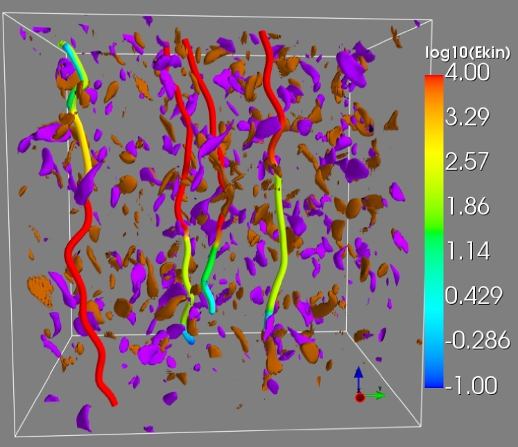
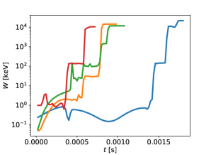
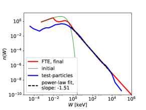
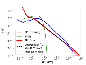
The acceleration process, is very efficient, and we consider a final time of s ( gyration periods), at which the asymptotic state has already been reached. Fig. 1 shows the component in the regions of above-critical current density, which clearly are fragmented into a large number of small-scale coherent structures within the nonlinear, super-Alfvénic MHD environment. The figure also shows the trajectories of 4 particles that reach high energies (MeV), and Fig. (2) shows the energy of the same 4 particles as a function of time. The particles can lose energy, yet they mostly gain energy in a number of sudden jumps in energy, the energization process thus is localized and there is multiple energization at different current filaments, as is also visible from the color-coded energy in Fig. 1. Fig. (2) shows the energy distribution at final time, which exhibits a clear power law part in the intermediate to high energy range with power-law index , with a slight turnover at the highest energies.
Transport coefficients and classical FP equation.
We now turn to the question whether the test-particle results can be reproduced as a solution of the FP equation. In order to simplify the FP equation (e.g. Gardiner (2004)), we neglect the spatial diffusion and consider particle diffusion only in energy space, including an escape term,
| (7) |
with the distribution function, the kinetic energy, and the escape time, and where is the energy diffusion coefficient,
| (8) |
and is the energy convection coefficient,
| (9) |
with a small time-interval. With we denote the conditional average that (see e.g. Ragwitz & Kantz (2001)). For the estimate of the coefficients, we follow the method described in Vlahos16 , i.e. we keep track of the energy of the particles at a number of monitoring times separated by , and to account for the conditional averaging, we divide the energies of the particles at time into a number of logarithmically equi-spaced bins and perform the requested averages separately for the particles in each bin.
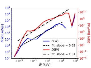
The estimates of and at s and as function of the energy are shown in Fig. 2, and they show a power-law shape, with power-law indexes and .
In Vlahos16 , we have shown that the described procedure of estimating the transport coefficients is consistent for the case of classical Fermi acceleration, in the sense that the test-particle distribution is reproduced quite well by the FP solution when the coefficients are inserted into the FP equation and the latter is solved numerically. We thus also here insert and , into the FP equation and solve it numerically in the energy interval , with the method described in Vlahos16 (pseudospectral method based on rational Chebyshev polynomials, combined with the backward Euler scheme, see e.g. Boyd (2001)). We also include the escape term, for which the escape time is estimated by assuming that the number of particles that stays inside the simulation box decays exponentially, which yields s.
The resulting evolution of the energy distribution up to a final time of s, is shown in Fig. (2). A clear power-law tail has developed, much flatter though than the one of the test-particle simulations. The discrepancy between the solution of the FP equation and the simulation data actually persists when applying larger integration times.
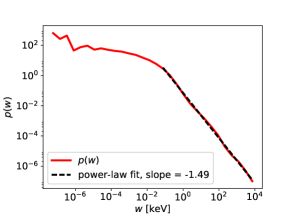
The failure of the classical FP equation can be explained by analyzing the sample of energy increments (with the particle index), on which the estimates of and are based (Eqs. (9) and (8)). These increments follow a power law distribution with index at intermediate to high energies, as shown in Fig. 2, and as a consequence the particles occasionally perform very large jumps in energy space (Levy flights), as illustrated in Fig. 2. The fact that the energy increments have a power-law distribution with the specific index has several consequences: (1) The estimates of as a mean value and as a variance theoretically are infinite, and thus in practice they are very problematic. (2) The mean is not representative for a scale-free power-law distribution. (3) The prerequisites for deriving a FP equation are not fulfilled, see the comments below.
Fractional transport equation (FTE).
A general description of transport in energy space is given by a variant of the Chapman-Kolmogorov equation
| (10) | |||||
see e.g. Klafter, Blumen & Shlesinger (1987); Klages, Radons, Sokolov (2008), which expresses a conservation law in energy space, and which can be interpreted as describing a Continuous Time Random Walk (CTRW) process. is the probability density for a particle to make a random walk step in energy, and the probability density for this step to be performed in a time interval , and for simplicity we have assumed the two probabilities to be independent. When both and are practically bounded, allowing only small increments, as e.g. if they are Gaussians, then the FP equation can be derived from Eq. (10) through Taylor-expansions (see e.g. Gardiner (2004)). For now, we do not make this smallness assumption.
A Fourier Laplace transform (, ), by applying the respective convolution theorems, yields
| (11) |
which is the Montroll-Weiss equation Montroll & Weiss (1965); Klafter, Blumen & Shlesinger (1987), written in non-standard form.
For the distribution of energy increments, expressed in Fourier space (i.e. the characteristic function), we consider the symmetric stable Levy distributions , with , which exhibit a power-law tail in energy-space, for and large, and for they are Gaussian distributions Hughes (1995). For the waiting time distribution, we assume one sided stable Levy distributions, expressed in Laplace space, with and , which have a power-law tail, for and large, and for they equal Hughes (1995).
In order to derive a meso-scopic equation, we consider the fluid-limit where are large, and thus are small, (e.g. Klages, Radons, Sokolov (2008), and references therein) so that the distributions of increments can be approximated as and . Upon inserting into Eq. (11), we find
| (12) |
which can be written as a fractional transport equation
| (13) |
with the Caputo fractional derivative of order , defined in Laplace space as
| (14) |
and the symmetric Riesz fractional derivative of order , defined in Fourier space as
| (15) |
see e.g. Klages, Radons, Sokolov (2008). Note that Eq. (13) includes the cases of a pure diffusion or convection equation ( and or 1, respectively). From the derivation of the FTE it is clear that the order of the fractional derivative is given by the index of the power-law tail of the distribution of increments, if any, otherwise, if the mean and variance of the increments are finite, then the classical FP equation is appropriate.
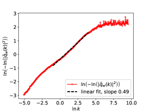
We need to estimate two parameter sets, , and , . can be inferred from the index of the power-law tail of in Fig. 2 as . As second method to determine and also , we use the characteristic function approach Borak05 ; Koutrouvelis80 , with the estimator of the characteristic function that is based on the sample of increments from the test-particle simulations,
| (16) |
for a suitable set of -values. If the obey a stable Levy distribution, then should hold, and a linear fit to as a function of will yield as the slope and as the intercept with the -axis. Fig. 2 shows , there indeed is a linear range, and we find and , with the value of being equal to the one inferred from the power-law tail of the increments.
We have probed the energy increments over a fixed time interval , and thus we considered the waiting time distribution to be , from which it follows that and . This approach seems unavoidable if the test-particle data are given in the form of time-series, where there is no direct information on the waiting times between scattering events. Thus, in the following we consider the transport equation to have an ordinary, first order derivative in time-direction and a fractional derivative in energy direction,
| (17) |
where we also have added an escape term.
For the numerical solution of the fractional transport equation, we use the Grünwald-Letnikov definition of fractional derivatives (e.g. Kilbas et al. (2006)) in the matrix formulation of Podlubny et al. (2009), and in order to use the same grid-points in as above for the solution of the classical FP equation, we use the derivative scheme given in Podlubny et al. (2013) for non equi-distant grid-points. Also, we apply the fractional derivative only above energies of eV, being interested here in the evolution of the high energy part, and considering that the FTE in its current form is not an appropriate tool to model low energy phenomena and heating, being motivated and derived here for modeling long tails at the high energy side of the energy distribution.
Fig. 2 shows the solution of the FTE at s, and obviously the distribution from the test-particle simulations is very well reproduced in what the power-law tail in its entire extent is concerned. Varying the anomalous resistivity from to , we find that the FTE we have introduced is always appropriate and successful in reproducing the simulation data (for no power-law tail is being formed).
Summary and Discussion.
It is to note that the statistical analysis of the simulation data, and in particular the analysis of the distribution of increments, plays a crucial role. First of all, this analysis allows to decide whether a classical FP equation or a FTE is appropriate.
In the case of anomalous transport, the data have to be analyzed statistically more in depth. The order of the fractional derivative is directly related to the index of the power-law tail of the increments and thus it is easy to estimate, and for an estimate of the scale parameter we have used the characteristic function method. After all, the form of the FTE and its parameters, most prominently the order of the fractional derivative, are directly inferred from the simulation data (and thus they are not universal or unique).
Also, we made no effort to model the low energy part of the distribution, which could possibly be achieved by combining the fractional term in the FTE with classical diffusive and convective terms.
Acknowledgements.
We would like to thank the anonymous referees for their constructive criticism. This work was supported by (a) the national Programme for the Controlled Thermonuclear Fusion, Hellenic Republic, (b) the EJP Cofund Action SEP-210130335 EUROfusion, and (c) the EUROfusion Consortium under grant agreement No 633053. The sponsors do not bear any responsibility for the content of this work.References
- Achterberg (1981) A. Achterberg, Astronomy & Astrophysics 97, 259 (1981).
- Arzner & Vlahos (2004) K. Arzner & L. Vlahos, The Astrophysical Journal Letters 605, L69 (2004).
- Biskamp & Welter (1989) D. Biskamp, & H. Welter, Physics of Fluids B 1, 1964 (1989).
- (4) S. Borak, W. Härdle, and R. Weron, in Statistical Tools for Finance and Insurance (Springer, 2005), pp. 21–44.
- Boyd (2001) J. P. Boyd, Chebyshev and Fourier spectral methods (Courier Corporation, 2001)
- Cargill et al. (2012) P. Cargill, L. Vlahos, G. Baumann, J. Drake & Å. Nordlund, Space science reviews 173, 223 (2012).
- Dahlin et al. (2015) J. T. Dahlin, J. F. Drake, & M. Swisdak, Physics of Plasmas 22, 100704 (2015).
- Dmitruk et al. (2004) P. Dmitruk, W.H. Matthaeus, & N. Seenu, Astrophys. J. 617, 667 (2004).
- Drake et al. (2006) J.F. Drake, M. Swisdak, H. Che, & M.A. Shay, Nature (London) 443, 553 (2006).
- Gardiner (2004) C.W. Gardiner, Handbook of Stochastic Methods, 4th ed. (Springer; Berlin & Heidelberg; 2009)
- (11) M. Gordovskyy, P.K. Browning, E.P. Kontar, and N.H. Bian, A&A 561, A72 (2014)
- (12) S. Gottlieb, C.-W. Shu, Mathematics of Computation 67, 73 (1998)
- Guo et al. (2015) F. Guo, Y.-H. Liu, W. Daughton, & H. Li, Astrophys. J. 806, 167 (2015).
- (14) M. Hoshino, Phys. Rev. Lett. 108, 135003 (2012).
- Hughes (1995) B.D. Hughes, Random Walks and Random Environments, Volume 1, Random Walks, Oxford (Clarendon Press, 1995).
- Kilbas et al. (2006) A.A. Kilbas, H.M. Srivastava, J.J. Trujillo, Theory and Applications of Fractional Differential Equations (Elsevier, Amsterdam, 2006).
- Klafter, Blumen & Shlesinger (1987) J. Klafter, A. Blumen, M.F. Shlesinger, Phys. Rev. A 35, 3081 (1987).
- Klages, Radons, Sokolov (2008) R. Klages, G. Radons, I.M. Sokolov, Anomalous Transport: Foundations and Applications (John Wiley & Sons, 2008).
- (19) I.A. Koutrouvelis, Journal of the American Statistical Association 75, 918 (1980).
- Kulsrud & Ferrari (1971) R. M. Kulsrud, A. Ferrari, Astrophysics and Space Science 12, 302 (1971).
- Lazarian & Vishniac (1999) A. Lazarian, & E.T. Vishniac, Astrophys. J. 517, 700 (1999)
- Matthaeus & Lamkin (1986) W.H. Matthaeus, & S.L. Lamkin, Physics of Fluids 29, 2513 (1986).
- Montroll & Weiss (1965) E.W. Montroll, G.H. Weiss, J. Math. Phys. 6, 167 (1965).
- Onofri et al. (2006) M. Onofri, H. Isliker, & L. Vlahos, Physical Review Letters 96, 151102 (2006).
- Petrosian (2012) V. Petrosian, Space science reviews 173, 535 (2012).
- Podlubny et al. (2009) I. Podlubny, A. Chechkin, T. Skovranek, Y.Q. Chen, B.M. Vinagre Jara, Journal of Computational Physics 228, 3137 (2009).
- Podlubny et al. (2013) I. Podlubny, T. Skovranek, B.M. Vinagre Jara, I. Petras, V. Verbitsky, Y.Q. Chen YQ., Phil Trans R Soc A 371, 20120153 (2013).
- Ragwitz & Kantz (2001) M. Ragwitz, & H. Kantz, Physical Review Letters 87, 254501 (2001).
- (29) X. Tao, A. A. Chan, and Alain J. Brizard, Phys. Plasmas 14, 092107 (2007).
- (30) L. Vlahos, Th. Pisokas, H. Isliker, V. Tsiolis, A. Anastasiadis, The Astrophysical Journal Letters 827, L3, (2016).
- (31) G. J. Morales and Y. C. Lee, Phys. Rev. Lett. 33, 1534 (1974).