Context Aware Document Embedding

Abstract

Recently, doc2vec has achieved excellent results in different tasks Lau and Baldwin (2016). In this paper, we present a context aware variant of doc2vec. We introduce a novel weight estimating mechanism that generates weights for each word occurrence according to its contribution in the context, using deep neural networks. Our context aware model can achieve similar results compared to doc2vec initialized by Wikipedia trained vectors, while being much more efficient and free from heavy external corpus. Analysis of context aware weights shows they are a kind of enhanced IDF weights that capture sub-topic level keywords in documents. They might result from deep neural networks that learn hidden representations with the least entropy.

1 Introduction

Knowledge representation, as a critical prerequisite for many machine learning tasks, has always been a central problem in the field of natural language processing (NLP). As for the representation of documents, an established form is to use bag-of-words (BOW) or term frequency-inverse document frequency (TF-IDF) representations. Another widely adopted method is generative topic models, such as latent semantic analysis (LSA) Deerwester et al. (1990) and latent dirichlet allocation (LDA) Blei et al. (2003).

Recently, Bengio et al. (2003) proposed a window-based unsupervised word embedding method. Following his approach, Mikolov et al. (2013a) introduced two new log-linear models, skip-gram and cbow. Mikolov et al. (2013b) gave a highly efficient implementation of those two models, and distributed it as word2vec, which has been widely used as a tool in language related tasks.

Inspired by the success of word2vec, Le and Mikolov (2014) extended word2vec into doc2vec, which produces a vector representation for each document, known as ”document embedding”. Dai et al. (2015) further examined doc2vec and found analogy features on Wikipedia (e.g. ”Lady Gaga” - ”American” + ”Japanese” $\approx$ ”Ayumi Hamasaki”). However, others have struggled to reproduce such results. Most recently, Lau and Baldwin (2016) made an empirical evaluation of doc2vec, and revealed its potential on different tasks.

Although doc2vec has produced promising results, we doubt its basis as it implicitly assigns the same weight to each word occurrence when training document vectors. This is counter-intuitive, since human never give equal attention to different parts of a sentence. Consider the following sentence as an example:

There are many activities
including but not limited to
running, jumping, and swimming.

When reading this sentence, we are not concerned about the ”there be” term. We will probably ignore ”limited to”, because ”including” and ”but not” indicate the parenthesis character of that term. The sentence can still be understood even if some parts are missing:

... many activities including
... running, jumping, ...

Motivated by such facts, we propose a context aware document embedding based on doc2vec. Our method takes a novel approach that estimates weights for each word occurrence by measuring the shift of the corresponding document vector if the word is substituted by another. We use convolutional neural networks (CNN) and gated recurrent units (GRU) as auxiliary models for the space of document vectors. We compared our model with benchmarks in Lau and Baldwin (2016) and doc2vec with IDF weights to show the advantage of our model. To give a convincing illustration of our model, we visualized the hidden states of deep neural networks. Our findings suggest that context aware weights are a kind of enhanced IDF weights that are especially good at capturing sub-topic level keywords in documents, since neural networks can substantially extract asymmetric context features, despite trained with unsupervisedly embedded targets.

2 Related Work

2.1 Distributed Bag of Words

The departure point of the context aware model is the distributed bag of word (DBOW) model of doc2vec proposed in Le and Mikolov (2014) trained with the negative sampling procedure Mikolov et al. (2013b). dbow uses a similar fashion like skip-gram Mikolov et al. (2013a) to train a document vector ($\mathbf{d}^{i}$) for each document with its context word vectors ($\mathbf{c}^{i}_{j}$). By adopting negative sampling procedure, the objective is to maximise the likelihood of $P(\mathbf{c}^{i}_{j}|\mathbf{d}^{i})$ while minimising the likelihood of $P(\mathbf{c}^{\prime}|\mathbf{d}^{i})$, where $\mathbf{c}^{\prime}$ is a random sample Goldberg and Levy (2014); Lau and Baldwin (2016). Therefore, the objective function is given as:

$$\sum_{j}{\left[\log\sigma({\mathbf{c}^{i}_{j}}^{\intercal}\mathbf{d}^{i})-\\ \sum_{k=1,\mathbf{c}^{\prime}\sim P_{n}(c)}^{n}{\log\sigma({\mathbf{c}^{\prime}}^{\intercal}\mathbf{d}^{i})}\right]}$$ (1)

where $\sigma$ is the sigmoid function, $n$ is the number of negative samples, and $P_{n}(c)$ is a distribution derived from term frequency.

Despite that dbow works with randomly initialized context word vectors, it is suggested that the quality of embeddings is improved when context word vectors are jointly trained by skip-gram and dbow Dai et al. (2015); Lau and Baldwin (2016). It is also observed that by initializing word vectors from pre-trained word2vec of large external corpus like wiki, the model converges faster as well as performs better Lau and Baldwin (2016).

2.2 CNN

Figure 1: CNN architecture

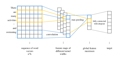
Convolutional neural networks (CNN) proposed by LeCun et al. (1998) are a kind of partially connected network architecture. CNN exploits convolution kernels to extract local features and uses pooling method to agglomerate features for subsequent layers, which have achieved excellent results in many NLP tasks Collobert et al. (2011); Yih et al. (2014). A typical CNN architecture for NLP consists of a convolutional layer, a global max pooling layer, and a fully connected layer , as is shown in Figure 1 Kim (2014).

For a document, the model takes a sequence of word vectors as input, and applies convolution along the sequence. The kernels are designed with different widths to extract features of different scales. Following each feature map, there is a max-pooling, which leads to a global maximum of the feature over the sequence. Finally, all features are concatenated and fully connected to the target, for either regression or classification purpose.

2.3 GRU

Figure 2: GRU architecture

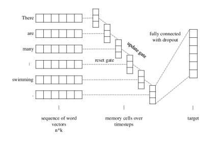
Gated recurrent units (GRU), introduced by Cho et al. (2014b, a); Chung et al. (2014), is a kind of recurrent neural networks (RNN) often used in semantics related tasks. An RNN is a neural network that scans input items one by one, and produces a representation for every prefix of the sequence, which can be formally written as

$$\mathbf{h}_{\left<t\right>}=f(\mathbf{h}_{\left<t-1\right>},\mathbf{x}_{t})$$

where $\mathbf{x}_{t}$ is the $t^{th}$ item, $\mathbf{h}_{\left<t\right>}$ is the hidden representation at timestep $t$, and $f$ is a non-linear activation function. In GRU, a reset gate $\mathbf{r}_{\left<t\right>}$ and an update gate $\mathbf{z}_{\left<t\right>}$ are used for regulating $f$.

$$\mathbf{z}_{\left<t\right>}=\sigma(\mathbf{W}_{z}\mathbf{x}_{t}+\mathbf{U}_{z}\mathbf{h}_{\left<t-1\right>})$$

$$\mathbf{r}_{\left<t\right>}=\sigma(\mathbf{W}_{r}\mathbf{x}_{t}+\mathbf{U}_{r}\mathbf{h}_{\left<t-1\right>})$$

where $\sigma$ is a non-negative activation function, usually sigmoid or hard sigmoid function. Then $f$ is computed by

$$f(\mathbf{h}_{\left<t-1\right>},\mathbf{x}_{t})=\mathbf{z}_{\left<t\right>}\odot\mathbf{h}_{\left<t-1\right>}+(1-\mathbf{z}_{\left<t\right>})\odot\tilde{\mathbf{h}}_{\left<t\right>}$$

with

$$\tilde{\mathbf{h}}_{\left<t\right>}=\phi\left(\mathbf{W}\mathbf{x}_{t}+\mathbf{U}(\mathbf{r}_{\left<t\right>}\odot\mathbf{h}_{\left<t-1\right>})\right)$$

where $\phi$ stands for $tanh$ function.

The two-gate design enables GRU to represent both long-term and short-term dependencies over timesteps. Units with update gate frequently activated tend to capture long-term dependencies, while units with reset gate activated tend to capture short-term dependencies Cho et al. (2014b). For regression targets over the sequence, a fully connected layer with dropout is added to the last timestep, as Figure 2 shows. ²

3 Context Aware Model

Our context aware model is an unsupervised model that trains doc2vec with word occurrence weights regarding their contexts. To generalize the problem, we will first define weighted dbow (notated as w-dbow), then illustrate the context aware model as a specific one of w-dbow.

A w-dbow model is defined as a triplet $(\mathcal{D},\mathcal{C},\mathcal{W})$. In the triplet, $\mathcal{D}$ and $\mathcal{C}$ are documents and context words for the vanilla doc2vec model, respectively. $\mathcal{W}$ is a set of weights corresponding to each word occurrence $\mathbf{c}\in\mathcal{C}$. Similar to Equation (1), the target is to minimize the following function:

$$\sum_{j}{\mathbf{w}^{i}_{j}\left[\log\sigma({\mathbf{c}^{i}_{j}}^{\intercal}\mathbf{d}^{i})-\sum_{k=1,\mathbf{c}^{\prime}\sim P_{n}(c)}^{n}{\log\sigma({\mathbf{c}^{\prime}}^{\intercal}\mathbf{d}^{i})}\right]}$$ (2)

where $\mathbf{w}^{i}_{j}\in\psi(\mathcal{W})$. Here we introduce a normalizing function $\psi$ on $\mathcal{W}$, because $\mathcal{W}$ may be scaled or biased in non-trivial cases. We adopt a global temperature softmax for $\psi$, which means

$$\psi(\mathbf{w}^{i}_{j})=\frac{|\mathcal{W}|e^{\mathbf{w}^{i}_{j}/T}}{\sum_{\mathbf{w}\in\mathcal{W}}{e^{\mathbf{w}/T}}}$$

$T$, known as the ”temperature”, is a hyperparameter that controls the softness of a softmax function. The result is scaled by $|\mathcal{W}|$ times so that the average $\mathbf{w}$ is $1$, which is the case in dbow. Therefore, hyperparameters like learning rate from dbow can be applied to w-dbow directly.

Input Size #Timesteps Output Size Loss Optimizer Epoch 300 93 300 cosine distance adam(lr=0.001) 100

Table 1: Shared hyperparameters of auxiliary models for STS task

The context aware model is a w-dbow that generates weights in the following way. First, a vanilla dbow is trained on the corpus, and then weight $\mathbf{w}^{i}_{j}$ is computed by randomly substitute $\mathbf{c}^{i}_{j}$ and measuring the shift in document vector $\mathbf{d}^{i}$ with cosine distance. This makes sense because there will be little shift if the word can be inferred from its context, otherwise a large shift should take place, as replacing the word impedes the meaning of the document. To predict document vectors on new word sequences, we trained an auxiliary model to regress document vectors with word vector sequences. We utilize CNN (Figure 1) and GRU (Figure 2) for this task. Hence, the corresponding context aware models are named as CA(CNN) and CA(GRU). Algorithm 1 gives details of this procedure

Algorithm 1 Generate context aware weights

1:$aux\_model\leftarrow$ CNN or GRU

2:$aux\_model.train(word\_sequence,doc)$

3:for $i\leftarrow 1$ to $|docs|$ do

4:     for $j\leftarrow 1$ to $|word\_sequence^{i}|$ do

5:         $shifts\leftarrow\varnothing$

6:         for $k\leftarrow 1$ to $sample\_count$ do

7:              $s^{\prime}\leftarrow word\_sequence^{i}$

8:              $s^{\prime}_{j}\leftarrow random\_word()$

9:              $d^{\prime}\leftarrow aux\_model.predict(s^{\prime})$

10:              $d\leftarrow doc^{i}$

11:              $shifts.add(cos\_distance(d^{\prime},d))$

12:         end for

13:         $\mathbf{w}^{i}_{j}\leftarrow average(shifts)$

14:     end for

15:end for

The weight is computed by averaging all the shifts of random substitutions. The random word is sampled from the global vocabulary with probability proportional to term frequency (TF). We also propose an economic way that take samples from words sharing the same part-of-speech (POS). Experiments show that two methods can achieve similar results, as will be shown in Section 4.

4 Experiments

4.1 Evaluation methods

We conduct experiments on the semantic textual similarity (STS) task. It is a shared task held by SemEval Agirre et al. (2015). In STS, the goal is to automatically predict a score for each sentence pair according to their semantic similarity. The result is evaluated by computing the Pearson correlation coefficient between the predicted score and the ground truth.

Since the official dataset provided by SemEval is quite small, we combine all datasets from 2012 to 2015 as the training set, following the approach in Lau and Baldwin (2016). We take the headlines domain of 2014 as the development set, and test on the 2015 dataset. It is reliable to specify the test set as a subset of the training set, as both our methods and baselines are unsupervised.

All datasets are preprocessed by lowercasing and tokenizing the sentence, using Stanford CoreNLP Manning et al. (2014). POS tags are also obtained through Stanford CoreNLP.

4.2 Baselines

To demonstrate the advantages of context aware models, we compare them with unsupervised baselines proposed in Lau and Baldwin (2016), including a linear combination of word vectors from skip-gram, and several dbow with different training settings. The linear combination computes a document embedding for a sentence by averaging over all its context with word vectors trained on the full collection of English Wikipedia entries.

For dbow, we train one model on the STS dataset. In the following context, we will refer these datasets as wiki and sts respectively. We train another model on wiki and exploit it to infer document vectors for sts without updating any hidden weights. ³

As it is observed in practice that using pretrained word vectors from external corpus can benefit the performance of dbow, we experiment a third dbow baseline with word vectors initialized by skip-gram trained on wiki. ^3,

Our context aware models are concrete implementations of w-dbow. Because w-dbow is consistent with dbow, we force context aware models to use the same hyperparameters as dbow. ⁴ We only optimise hyperparameters of the auxiliary model (i.e. CNN or GRU) towards the target of document vectors through cross-validation on the training set, as well as the temperature $T$ on the development set. In the following context, these two methods are referred as CA(CNN) and CA(GRU) respectively.

To distinguish context aware models from other weighting methods, we also introduced a w-dbow baseline with weights from inverse document frequency (IDF) as w-dbow(IDF). We optimise its temperature $T$ separately from context aware models.

4.3 Experiments

Domain skip-gram dbow CA(CNN) CA(GRU) w-dbow(IDF) wiki sts wiki sts (wiki init) sts sts answers-forums 0.516 0.647 0.666 0.675 0.670 0.662 0.656 headlines 0.731 0.768 0.746 0.782 0.785 0.787 0.788 answers-students 0.661 0.640 0.628 0.654 0.683 0.676 0.660 belief 0.607 0.764 0.713 0.773 0.772 0.764 0.760 images 0.678 0.781 0.789 0.800 0.793 0.793 0.787

Table 2: Results over STS task with different unsupervised methods

Domain CA(CNN) CA(GRU) global POS global POS answers-forums 0.663 0.670 0.668 0.662 headlines 0.786 0.785 0.786 0.787 answers-students 0.673 0.683 0.675 0.676 belief 0.760 0.772 0.761 0.764 images 0.800 0.793 0.792 0.793

Table 3: Context aware models with random sampling from different distributions. The global distribution is proportional to TF of each word. The POS distribution is proportional to TF of each word grouped by POS. Samples are taken from the corresponding distribution regarding POS of the substituted word. We take 50 and 10 samples for global distribution and POS distribution respectively.

First, we decide hyperparameters for our auxiliary models. For CNN, it is observed through cross-validation that kernels with width from 3 to 8 best capture features from the word vector sequence to make the vanilla document vector. Considering the scale of sts dataset, we use 128 kernels for each width. For GRU, we use 512 hidden units. Both deep networks have 1.4M trainable parameters approximately, indicating they should have the same capability.

Then we optimise the temperature $T$ for w-dbow models. We find that results on the development set almost follows a unimodal function as $T$ varies, which facilitates the optimization of $T$ a lot. In general, $T$ around 1/15–1/14 works for both CA(CNN) and CA(GRU), while $T$ around 5–6 works for w-dbow(IDF).

Experiments show that our context aware models outperforms dbow in all 5 domains (Table 2). Of two purposed models, CA(CNN) works a little better and results at the same level of dbow initialized by word vectors from wiki. Besides, w-dbow(IDF) also gets a better performance than dbow, which buttresses the consistency of our definition for w-dbow. More interestingly, all w-dbow baselines make excellent results in the domain of answers-students, compared to any dbow approach. We will give a detailed analysis of this in Section 5.

We also compared CA(CNN) and CA(GRU) with different word distributions. Table 3 gives results in detail. Consistent with our estimation, the difference between global distribution and POS distribution is not significant. Therefore, gain of context aware models comes from weighting method rather than sampling from POS distribution. However, we recommend to use POS distribution for random substitution, as it is much smaller and more efficient.

5 Model Introspection

(a) dbow

(b) dbow (wiki init)

(c) CA(CNN)

(d) CA(GRU)

(e) w-dbow(IDF)

Figure 3: Distribution of different document vectors under t-SNE

Figure 4: A sample of weights learned by the context aware model. Brighter bars denote larger weights.

Being unsupervised models, our context aware models surpass the vanilla dbow, and even show some advantage towards dbow (wiki init). This is momentous because context aware models only exploit the local corpus, without external priori like pretrained vectors. Hence, we believe context aware models do extract more information from the corpus. We will shed some light on why and how context aware models work by looking into document vectors and hidden representations of the model.

In context aware models, weights learned by word-level substitution consists of two components. One is a base value for each word, the other is a context-related bias for each word occurrence. The base value is something close to IDF, as there is a moderate correlation between context aware weights and IDF. Hence, context aware models can be viewed as an enhanced version of w-dbow(IDF).

Generally, both context aware models and w-dbow(IDF) give equal or smaller similarity answers in STS task. They tend to distinguish sentences rather than find trivial similarities. In other words, IDF weighted loss makes document embeddings insensitive to common words. Context aware models even enable them to neglect common words given the context in a self-adaptive manner, which is very similar to lateral inhibition in cognition and neuroscience.

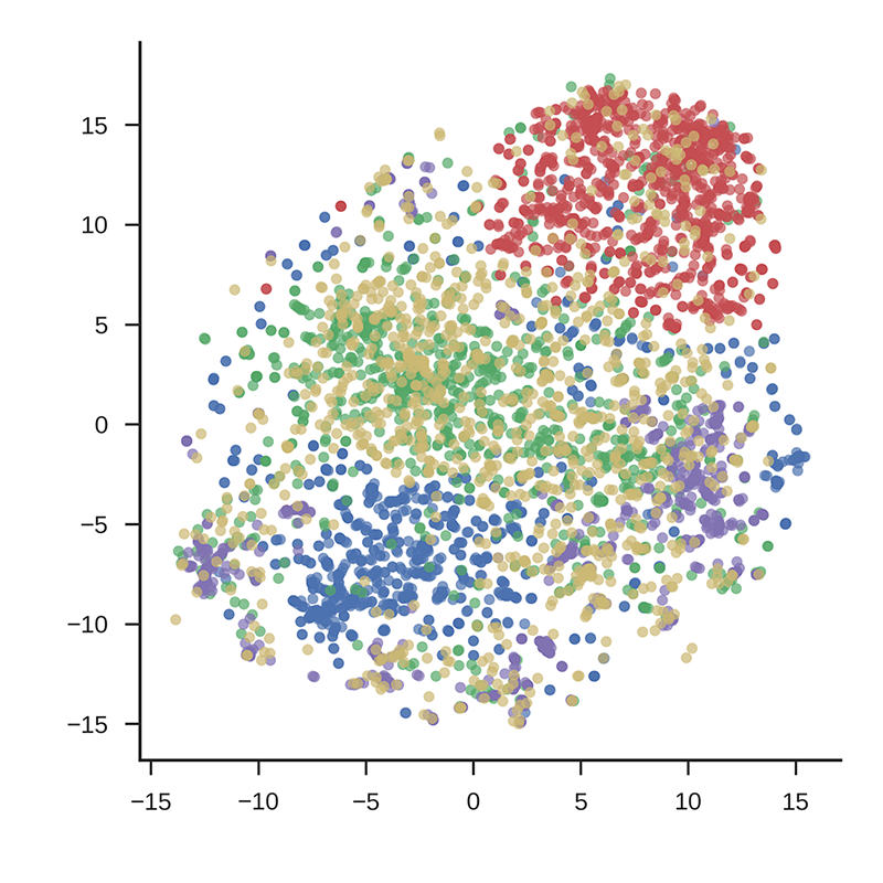
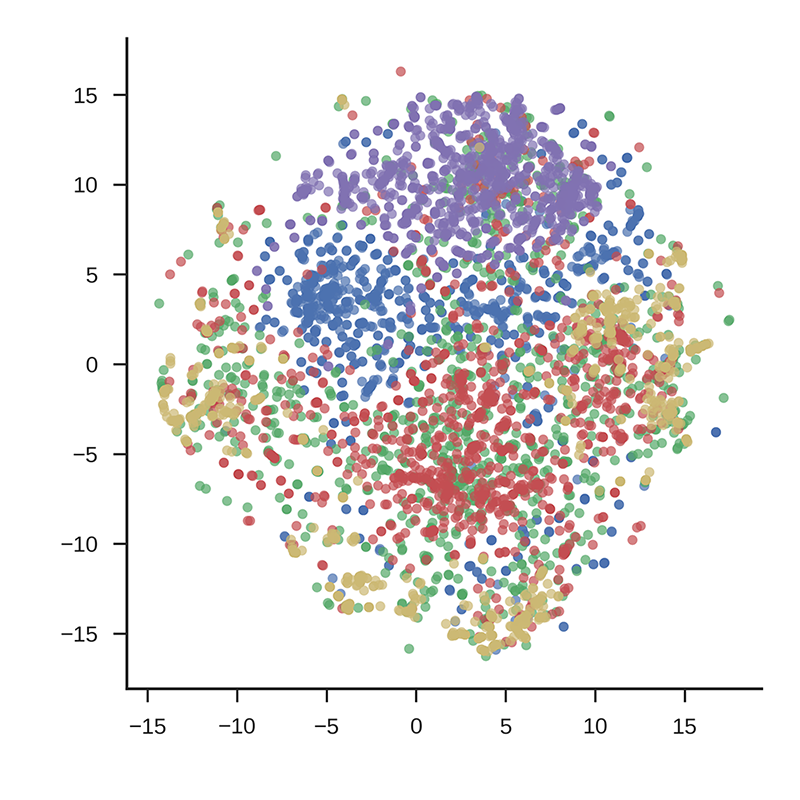
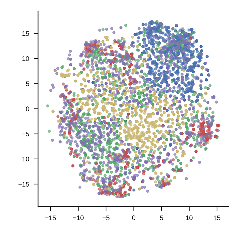
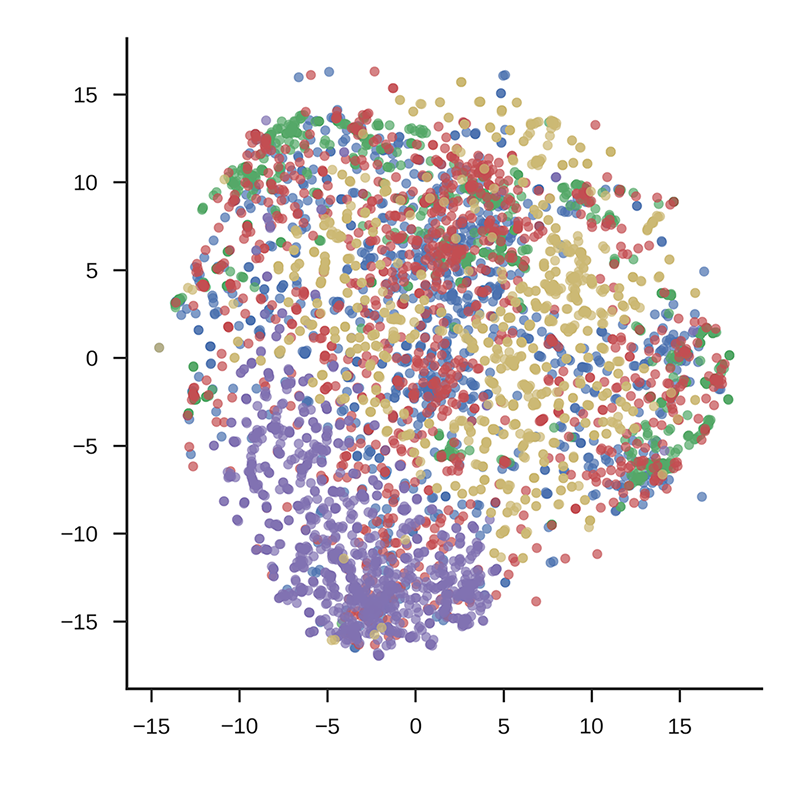
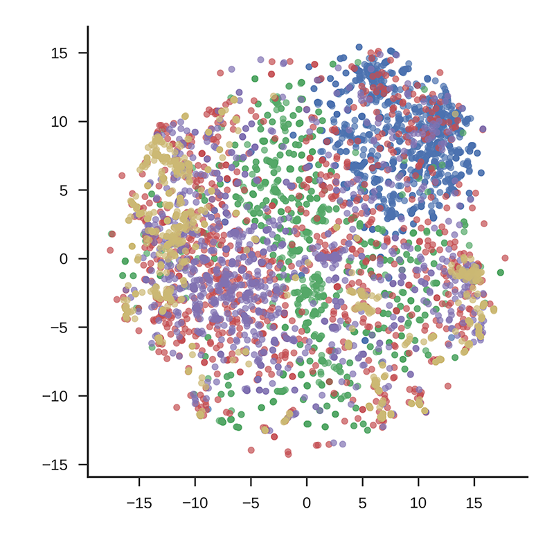
To illustrate this, consider the distribution of document vectors on the test set using t-SNE Maaten and Hinton (2008) in Figure 3. Document vectors of different domains are marked with different colors. Since domains are natural categories, dots of the same color should gather as a cluster. Consistent with our experience, dbow forms good clusters. However, none of three w-dbow models gives such a clear result. In context aware embeddings, though clusters still can be observed, a number of dots are scattered far away from their centers. The phenomenon is extremely significant in answers-students (red), where dbow performs worst and context aware models improve most. This might be attributed to that different from coarse-grained task like clustering, STS task more relies on fine-grained features, where our models have advantage over vanilla dbow.

We then examine the domain of answers-students. It contains students answer to electricity problems, of which most share the same topic, but their semantic similarity varies. As for a concrete example, we randomly pick a sentence pair from answers-students whose similarity differs much in dbow and context aware models. Figure 4 clearly shows weights learned by CA(CNN). It can be spotted that low weights are assigned to common words. Moreover, context aware model neglects jargons like ”voltage” or ”terminal”, but focuses on ”difference”, which is a relatively rare occurrence given the context. In fact, it is word like ”difference” and ”positive” that defines the key point of a sentence in a topic. With context aware weights, their contribution are well amplified.

Context word CNN GRU IDF #feature change norm of $\mathbf{r}_{\left<t\right>}$ Voltage 393 5.037 5.805 is 157 8.847 1.526 the 98 10.168 0.877 difference 385 7.153 5.925 between 200 8.957 4.678 a 96 10.039 0.953 positive 324 5.916 4.383 and 99 9.334 1.671 negative 322 6.017 5.363 terminal 328 5.393 4.066 on 122 10.349 2.171 the 53 10.476 0.877 battery 230 6.889 3.422 . 15 10.570 0.417 Correlation to IDF 0.915 -0.845 1

Table 4: Influence of each context word on hidden representations

Notice that auxiliary models are trained with document vectors, which are generated according to context words homogeneously. But shifts in the vector space do behave heterogeneously regard to each substituted occurrence. To find the origin of such asymmetry, we investigate on the hidden states of auxiliary models. For CNN, we count the number of global features that change in substitution. For GRU, since the hidden representation varies in different timesteps, we count the norm of $\mathbf{r}_{\left<t\right>}$, as it implies how much units ”decline” the input. Surprisingly, both auxiliary models reveal unequal hidden states, as shown in Table 4. The number of features that a word contributes to in CNN is highly correlated with its IDF, while the extent to which hidden units turn down a word in GRU is highly negatively correlated with its IDF. Since IDF is the entropy of every word given its distribution over a corpus, we are inclined to believe that the first layer of deep neural networks learns hidden representations towards the least entropy over the corpus (i.e. maximize the use of hidden units).

6 Conclusion

We introduce two context aware models for document embedding with a novel weight estimating mechanism. Compared to vanilla dbow method, our approach infers a weight for each word occurrence with regard to its context, which helps document embedding to capture sub-topic level keywords. This property facilitates learning a more fine-grained embedding for semantic textual similarity task as well as eases training on large external corpus. We claim that context aware weights is composed of an IDF base and a context-related bias. This might be induced by deep neural networks as they naturally learns representations with the least entropy, even when the target is generated homogeneously.

References

- Agirre et al. (2015) Eneko Agirre, Carmen Baneab, Claire Cardiec, Daniel Cerd, Mona Diabe, Aitor Gonzalez-Agirrea, Weiwei Guof, Inigo Lopez-Gazpioa, Montse Maritxalara, Rada Mihalceab, et al. 2015. Semeval-2015 task 2: Semantic textual similarity, english, spanish and pilot on interpretability. In Proceedings of the 9th international workshop on semantic evaluation (SemEval 2015). pages 252–263.
- Bengio et al. (2003) Yoshua Bengio, Réjean Ducharme, Pascal Vincent, and Christian Jauvin. 2003. A neural probabilistic language model. Journal of machine learning research (JMLR) 3(Feb):1137–1155.
- Blei et al. (2003) David M Blei, Andrew Y Ng, and Michael I Jordan. 2003. Latent dirichlet allocation. Journal of machine Learning research (JMLR) 3(Jan):993–1022.
- Cho et al. (2014a) Kyunghyun Cho, Bart van Merriënboer, Dzmitry Bahdanau, and Yoshua Bengio. 2014a. On the properties of neural machine translation: Encoder–decoder approaches. Syntax, Semantics and Structure in Statistical Translation page 103.
- Cho et al. (2014b) Kyunghyun Cho, Bart Van Merriënboer, Caglar Gulcehre, Dzmitry Bahdanau, Fethi Bougares, Holger Schwenk, and Yoshua Bengio. 2014b. Learning phrase representations using rnn encoder-decoder for statistical machine translation. In Proceedings of the 2014 Conference on Empirical Methods in Natural Language Processing (EMNLP). pages 1724–1734.
- Chollet (2015) François Chollet. 2015. Keras.
- Chung et al. (2014) Junyoung Chung, Caglar Gulcehre, KyungHyun Cho, and Yoshua Bengio. 2014. Empirical evaluation of gated recurrent neural networks on sequence modeling. NIPS Deep Learning Workshop .
- Collobert et al. (2011) Ronan Collobert, Jason Weston, Léon Bottou, Michael Karlen, Koray Kavukcuoglu, and Pavel Kuksa. 2011. Natural language processing (almost) from scratch. Journal of Machine Learning Research 12(Aug):2493–2537.
- Dai et al. (2015) Andrew M Dai, Christopher Olah, and Quoc V Le. 2015. Document embedding with paragraph vectors. NIPS Deep Learning Workshop .
- Deerwester et al. (1990) Scott Deerwester, Susan T Dumais, George W Furnas, Thomas K Landauer, and Richard Harshman. 1990. Indexing by latent semantic analysis. Journal of the American society for information science 41(6):391.
- Goldberg and Levy (2014) Yoav Goldberg and Omer Levy. 2014. word2vec explained: Deriving mikolov et al.’s negative-sampling word-embedding method. arXiv preprint arXiv:1402.3722 .
- Kim (2014) Yoon Kim. 2014. Convolutional neural networks for sentence classification. In Proceedings of the 2014 Conference on Empirical Methods in Natural Language Processing (EMNLP). pages 1746–1751.
- Lau and Baldwin (2016) Jey Han Lau and Timothy Baldwin. 2016. An empirical evaluation of doc2vec with practical insights into document embedding generation. Association for Computational Linguistics (ACL) page 78.
- Le and Mikolov (2014) Quoc V Le and Tomas Mikolov. 2014. Distributed representations of sentences and documents. In Proceedings of the 31st International Conference on Machine Learning (ICML). volume 14, pages 1188–1196.
- LeCun et al. (1998) Yann LeCun, Léon Bottou, Yoshua Bengio, and Patrick Haffner. 1998. Gradient-based learning applied to document recognition. Proceedings of the IEEE 86(11):2278–2324.
- Maaten and Hinton (2008) Laurens van der Maaten and Geoffrey Hinton. 2008. Visualizing data using t-sne. Journal of Machine Learning Research 9(Nov):2579–2605.
- Manning et al. (2014) Christopher D Manning, Mihai Surdeanu, John Bauer, Jenny Rose Finkel, Steven Bethard, and David McClosky. 2014. The stanford corenlp natural language processing toolkit. In Association for Computational Linguistics (ACL) System Demonstrations. pages 55–60.
- Mikolov et al. (2013a) Tomas Mikolov, Kai Chen, Greg Corrado, and Jeffrey Dean. 2013a. Efficient estimation of word representations in vector space. International Conference on Learning Representations (ICLR) .
- Mikolov et al. (2013b) Tomas Mikolov, Ilya Sutskever, Kai Chen, Greg S Corrado, and Jeff Dean. 2013b. Distributed representations of words and phrases and their compositionality. In Advances in neural information processing systems (NIPS). pages 3111–3119.
- Pennington et al. (2014) Jeffrey Pennington, Richard Socher, and Christopher D Manning. 2014. Glove: Global vectors for word representation. In Proceedings of the 2014 Conference on Empirical Methods in Natural Language Processing (EMNLP). volume 14, pages 1532–1543.
- Rehurek and Sojka (2010) Radim Rehurek and Petr Sojka. 2010. Software framework for topic modelling with large corpora. In In Proceedings of the LREC 2010 Workshop on New Challenges for NLP Frameworks. Citeseer.
- Yih et al. (2014) Wen-tau Yih, Xiaodong He, and Christopher Meek. 2014. Semantic parsing for single-relation question answering. In Association for Computational Linguistics (ACL). Citeseer, pages 643–648.
- Zhang et al. (2017) Chiyuan Zhang, Samy Bengio, Moritz Hardt, Benjamin Recht, and Oriol Vinyals. 2017. Understanding deep learning requires rethinking generalization.