Synthesis of Data Completion Scripts using Finite Tree Automata

Abstract.

In application domains that store data in a tabular format, a common task is to fill the values of some cells using values stored in other cells. For instance, such data completion tasks arise in the context of missing value imputation in data science and derived data computation in spreadsheets and relational databases. Unfortunately, end-users and data scientists typically struggle with many data completion tasks that require non-trivial programming expertise. This paper presents a synthesis technique for automating data completion tasks using programming-by-example (PBE) and a very lightweight sketching approach. Given a formula sketch (e.g., AVG($\textnormal{{?}}_{1}$, $\textnormal{{?}}_{2}$)) and a few input-output examples for each hole, our technique synthesizes a program to automate the desired data completion task. Towards this goal, we propose a domain-specific language (DSL) that combines spatial and relational reasoning over tabular data and a novel synthesis algorithm that can generate DSL programs that are consistent with the input-output examples. The key technical novelty of our approach is a new version space learning algorithm that is based on finite tree automata (FTA). The use of FTAs in the learning algorithm leads to a more compact representation that allows more sharing between programs that are consistent with the examples. We have implemented the proposed approach in a tool called DACE and evaluate it on 84 benchmarks taken from online help forums. We also illustrate the advantages of our approach by comparing our technique against two existing synthesizers, namely PROSE and SKETCH.

1. Introduction

Many application domains store data in a tabular form arranged using rows and columns. For example, Excel spreadsheets, R dataframes, and relational databases all view the underlying data as a 2-dimensional table consisting of cells. In this context, a common scenario is to fill the values of some cells using values stored in other cells. For instance, consider the following common data completion tasks:

• Data imputation: In statistics, imputation means replacing missing data with substituted values. Since missing values can hinder data analytics tasks, users often need to fill missing values using other related entries in the table. For instance, data imputation arises frequently in statistical computing frameworks, such as R and pandas.

• Spreadsheet computation: In many applications involving spreadsheets, users need to calculate the value of a cell based on values from other cells. For instance, a common task is to introduce new columns, where each value in the new column is derived from values in existing columns.

• Virtual columns in databases: In relational databases, users sometimes create views that store the result of some database query. In this context, a common task is to add virtual columns whose values are computed using existing entries in the view.

As illustrated by these examples, users often need to complete missing values in tabular data. While some of these data completion tasks are fairly straightforward, many others require non-trivial programming knowledge that is beyond the expertise of end-users and data scientists.

To illustrate a typical data completion task, consider the tabular data shown in Fig. 1. Here, the table stores measurements for different people during a certain time period, where each row represents a person and each column corresponds to a day. As explained in a StackOverflow post , a data scientist analyzing this data wants to compute the difference of the measurements between the first and last days for each person and record this information in the Delta column. Since the table contains a large number of rows (of which only a small subset is shown in Fig. 1), manually computing this data is prohibitively cumbersome. Furthermore, since each person’s start and end date is different, automating this data completion requires non-trivial programming logic.

Figure 1. A data completion task taken from StackOverflow.

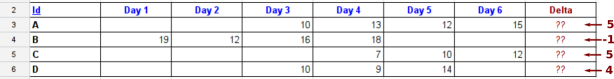
In this paper, we present a novel program synthesis technique for automating data completion tasks in tabular data sources, such as dataframes, spreadsheets, and relational databases. Our synthesis methodology is based on two key insights that we gained by analyzing dozens of posts on online forums: First, it is often easy for end-users to specify which operators should be used in the data completion task and provide a specific instantiation of the operands for a few example cells. However, it is typically very difficult for end-users to express the general operand extraction logic. For instance, for the example from Fig. 1, the user knows that the missing value can be computed as $C_{1}-C_{2}$, but he is not sure how to implement the logic for extracting $C_{1},C_{2}$ in the general case.

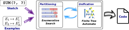
Based on this observation, our synthesis methodology for data completion combines program sketching and programming-by-example (PBE). Specifically, given a formula sketch (e.g., SUM($\textnormal{{?}}_{1}$,AVG($\textnormal{{?}}_{2}$,$\textnormal{{?}}_{3}$))) as well as a few input-output examples for each hole, our technique automatically synthesizes a program that can be used to fill all missing values in the table. For instance, in our running example, the user provides the sketch MINUS($\textnormal{{?}}_{1}$,$\textnormal{{?}}_{2}$) as well as the following input-output examples for the two holes:

$\textnormal{{?}}_{1}$	$\textnormal{{?}}_{2}$
(A, Delta) $\mapsto$ (A, Day 6)	(A, Delta) $\mapsto$ (A, Day 3)
(B, Delta) $\mapsto$ (B, Day 4)	(B, Delta) $\mapsto$ (B, Day 1)

Given these examples, our technique automatically synthesizes a program that can be used to fill all values in the Delta column in Fig. 1.

One of the key pillars underlying our synthesis algorithm is the design of a new domain-specific language (DSL) that is expressive enough to capture most data completion tasks we have encountered, yet lightweight enough to facilitate automation. The programs in our DSL take as input a table and a cell with missing value, and return a list of cells that are used for computing the missing value. Our main insight in designing this DSL is to use abstractions that combine spatial reasoning in the tabular structure with relational reasoning. Spatial reasoning allows the DSL programs to follow structured paths in the 2-dimensional table whereas relational reasoning allows them to constrain those paths with predicates over cell values.

As shown schematically in Fig. 2, the high-level structure of our synthesis algorithm is similar to prior techniques that combine partitioning with unification (Gulwani, 2011; Yaghmazadeh et al., 2016; Alur et al., 2015) . Specifically, partitioning is used to classify the input-output examples into a small number of groups, each of which can be represented using a conditional-free program in the DSL. In contrast, the goal of unification is to find a conditional-free program that is consistent with each example in the group. The key novelty of our synthesis algorithm is a new unification algorithm based on finite tree automata (FTA).

Our unification procedure can be viewed as a new version space learning algorithm (Mitchell, 1982) that succinctly represents a large number of programs. Specifically, a version space represents all viable hypotheses that are consistent with a given set of examples, and prior work on programming-by-example have used so-called version space algebras (VSA) to combine simpler version spaces into more complex ones (Lau et al., 2003; Gulwani, 2011; Polozov and Gulwani, 2015). Our use of FTAs for version space learning offers several advantages compared to prior VSA-based techniques such as PROSE: First, FTAs represent version spaces more succinctly, without explicitly constructing individual sub-spaces representing sub-expressions. Hence, our approach avoids the need for finite unrolling of recursive expressions in the DSL. Second, our finite-tree automata are constructed in a forward manner using the DSL semantics. In constrast to VSA-based approaches such as PROSE that construct VSAs in a backward fashion starting from the outputs, our approach therefore obviates the need to manually define complex inverse semantics for each DSL construct. As we demonstrate experimentally, our version space learning algorithm using FTAs significantly outperforms the VSA-based learning algorithm used in PROSE.

Figure 2. High-level overview of our synthesis approach.

We have implemented our synthesis algorithm in a tool called DACE  and evaluated it on $84$ real-world data completion tasks collected from online help forums. Our evaluation shows that DACE can successfully synthesize over $92\%$ of the data completion tasks in an average of $0.7$ seconds. We also empirically compare our approach against PROSE and SKETCH and show that our new synthesis technique outperforms these baseline algorithms by orders of magnitude in the data completion domain.

To summarize, this paper makes the following key contributions:

• We propose a new program synthesis methodology that combines program sketching and programming-by-example techniques to automate a large class of data completion tasks involving tabular data.

• We describe a DSL that can concisely express a large class of data completion tasks and that is amenable to an efficient synthesis algorithm.

• We propose a new unification algorithm that uses finite tree automata to construct version spaces that succinctly represent DSL programs that are consistent with a set of input-output examples.

• We evaluate our approach on real-world data completion tasks involving dataframes, spreadsheets, and relational databases. Our experiments show that the proposed learning algorithm is effective in practice.

2. Motivating Examples

In this section, we present some representative data completion tasks collected from online help forums. Our main goal here is to demonstrate the diversity of data completion tasks and motivate various design choices for the DSL of cell extraction programs.

Example 2.1.

A numerical ecologist needs to perform data imputation in R using the last observation carried forward (LOCF) method . Specifically, he would like to replace each missing entry with the previous non-missing entry incremented by $1$. For instance, if the original row contains $[2,2,\textnormal{{?}},\textnormal{{?}},8,\textnormal{{?}}]$, the new row should be $[2,2,3,3,8,9]$.

Here, the desired imputation task can be expressed using the simple formula sketch $\texttt{SUM}(\textnormal{{?}}_{1},1)$. The synthesis task is to find an expression that retrieves the previous non-missing value for each missing entry.

Example 2.2.

An astronomer needs to perform data imputation using Python’s pandas data analysis library . Specifically, the astronomer wants to replace each missing value with the previous non-missing value with the same id. The desired data imputation task is illustrated in Fig. 3(a).

As this example illustrates, some data completion tasks require finding a cell that satisfies a relational predicate. In this case, the desired cell with non-missing value must have the same id as the id of the cell with missing value.

1 2 1: id x 2: $1$ $10$ 3: $1$ $\textnormal{{?}}\shortleftarrow 10$ 4: $2$ $100$ 5: $2$ $200$ 6: $1$ $\textnormal{{?}}\shortleftarrow 10$ 7: $2$ $\textnormal{{?}}\shortleftarrow 200$ 8: $1$ $300$ $\cdot\cdot$ $\cdot\cdot$			1 2 3 4 1: 2016-11-01 A $\textnormal{{?}}\shortleftarrow 12$ $\textnormal{{?}}\shortleftarrow 200$ 2: 2016-11-02 B $12$ $\textnormal{{?}}\shortleftarrow 200$ 3: 2016-11-03 A $\textnormal{{?}}\shortleftarrow 12$ $200$ 4: 2016-11-04 C $18$ $400$ 5: 2016-11-05 B $10$ $\textnormal{{?}}\shortleftarrow 400$ 6: 2016-11-06 B $\textnormal{{?}}\shortleftarrow 10$ $800$ 7: 2016-11-07 C $\textnormal{{?}}\shortleftarrow 10$ $1000$ $\cdot\cdot$ $\cdot\cdot$ $\cdot\cdot$ $\cdot\cdot$
(a)	(b)	(c)	(d)

Figure 3. (a) Replace missing entry by previous non-missing value with same id. (b) Fill cells in column D by copying values in column C. (c) Calculate total count for each group. (d) Replace missing value by previous non-missing value (if exists), otherwise use next non-missing one.

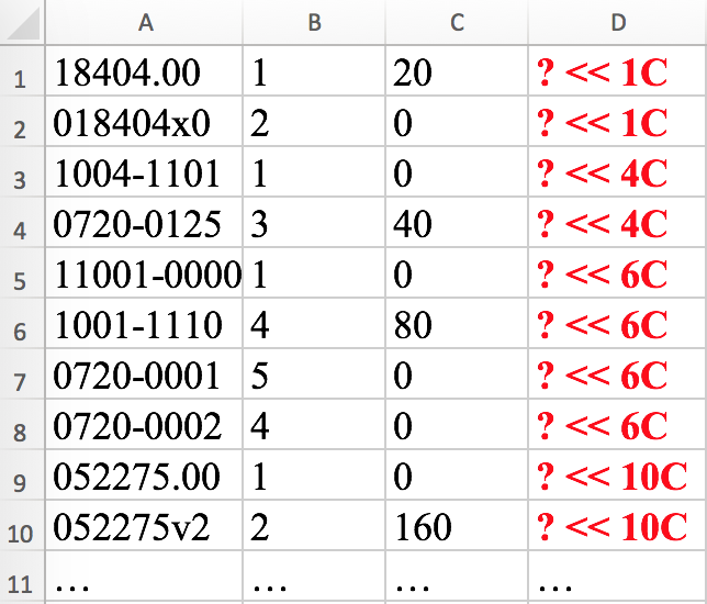
Example 2.3.

A businessman using Excel wants to add a new column to his spreadsheet . As shown in Fig. 3 (b), the entries in the new column D are obtained from column C. Specifically, the data completion logic is as follows: First, find the previous row that has value $1$ in column $B$. Then, go down from that row and find the first non-zero value in column $C$ and use that value to populate the cell in column $D$. Fig. 3 (b) shows the desired values for column $D$.

As this example illustrates, the cell extraction logic in some tasks can be quite involved. In this example, we first need to find an intermediate cell satisfying a certain property (namely, it must be upwards from the missing cell and have value $1$ in column $B$). Then, once we find this intermediate cell, we need to find the target cell satisfying a different property (namely, it must be downwards from the intermediate cell and store a non-zero value in column $C$).

This example illustrates two important points: First, the data extraction logic can combine both geometric (upward and downward search) and relational properties. Second, the data extraction logic can require “making turns” — in this example, we first go up to an intermediate cell and then change direction by going down to find the target cell using a different logic.

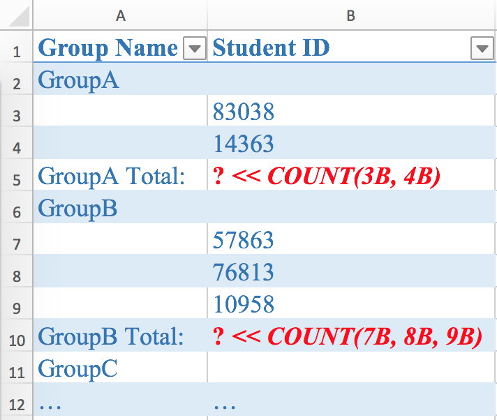
Example 2.4.

A statistician working on spreadsheet data needs to complete the “Group Total” rows from Fig. 3 (c) using the count of entries in that group . For instance, the GroupA Total entry should be filled with $2$.

This example illustrates the need for allowing holes of type list in the sketches. Since each missing value is obtained by counting a variable number of entries, the user instead provides a sketch $\texttt{COUNT}(\textnormal{{?}}_{1})$, where $\textnormal{{?}}_{1}$ represents a list of cells. Furthermore, this example also illustrates the need for a language construct that can extract a range of values satisfying a certain property. For instance, in this example, we need to extract all cells between the cell $c$ to be completed and the first empty entry that is upwards from $c$.

Example 2.5.

An R user wants to perform imputation on the dataframe shown in Fig. 3 (d) using the LOCF method. Specifically, she wants to impute the missing value by substituting it with the first previous non-missing value in the same column. However, if no such entry exists, she wants to fill the missing entry by using the first following non-missing value in the same column instead.

This example illustrates the need for allowing a conditional construct in our DSL: Here, we first try some extraction logic, and, if it fails, we then resort to a back-up strategy. Many of the data completion tasks that we have encountered follow this pattern – i.e., they try different extraction logics depending on whether the previous logic succeeds. Based on this observation, our DSL introduces a restricted form of switch statement, where the conditional implicitly checks if the current branch fails.

3. Specifications

Task	Sketch	Input-output examples
Example 2.1	$\texttt{SUM}(\textnormal{{?}}_{1},1)$	$\big{\{}\textnormal{{?}}_{1}\hookrightarrow\{(1,3)\mapsto[(1,2)],(1,4)\mapsto[(1,2)],(1,6)\mapsto[(1,5)]\}\big{\}}$
Example 2.2	$\textnormal{{?}}_{1}$	$\big{\{}\textnormal{{?}}_{1}\hookrightarrow\{(3,2)\mapsto[(2,2)],(6,2)\mapsto[(2,2)],(7,2)\mapsto[(5,2)]\}\big{\}}$
Example 2.3	$\textnormal{{?}}_{1}$	$\big{\{}\textnormal{{?}}_{1}\hookrightarrow\{(1,D)\mapsto[(1,C)],(3,D)\mapsto[(4,C)],(8,D)\mapsto[(6,C)]\}\big{\}}$
Example 2.4	$\texttt{COUNT}(\textnormal{{?}}_{1})$	$\big{\{}\textnormal{{?}}_{1}\hookrightarrow\{(5,B)\mapsto[(3,B),(4,B)],(10,B)\mapsto[(7,B),(8,B),(9,B)]\}\big{\}}$
Example 2.5	$\textnormal{{?}}_{1}$	$\big{\{}\textnormal{{?}}_{1}\hookrightarrow\{(3,3)\mapsto[(2,3)],(7,3)\mapsto[(5,3)],(1,4)\mapsto[(3,4)]\}\big{\}}$

Figure 4. Specifications for examples from Section 2.

A specification in our synthesis methodology is a pair $(\mathcal{S},\mathcal{E})$, where $\mathcal{S}$ is a formula sketch and $\mathcal{E}$ is a set of input-output examples. Specifically, formula sketches are defined by the following grammar:

$$\begin{array}[]{lll}\text{Sketch}~{}\mathcal{S}&:=&t~{}|~{}F(\mathcal{S}_{1},\cdot\cdot,\mathcal{S}_{n}),\ \ \ F\in\Lambda\\ \text{Term}~{}t&:=&const~{}|~{}\textnormal{{?}}_{id}\\ \end{array}$$

Here, $\Lambda$ denotes a family of pre-defined functions, such as AVG, SUM, MAX, etc. Holes in the sketch represent unknown cell extraction programs to be synthesized. Observe that formula sketches can contain multiple functions. For instance, ${\tt SUM}({\tt MAX}(\textnormal{{?}}_{1},\textnormal{{?}}_{2}),1)$ is a valid sketch and indicates that a missing value in the table should be filled by adding one to the maximum of two unknown cells.

In many cases, the data completion task involves copying values from an existing cell. In this case, the user can express her intent using the identity sketch ${\tt ID}(\textnormal{{?}}_{1})$. Since this sketch is quite common, we abbreviate it using the notation $\textnormal{{?}}_{1}$.

In addition to the sketch, users of DACE are also expected to provide one or more input-output examples $\mathcal{E}$ for each hole. Specifically, examples $\mathcal{E}$ map each hole $\textnormal{{?}}_{id}$ in the sketch to a set of pairs of the form $i\mapsto[o_{1},\cdot\cdot,o_{n}]$, where $i$ is an input cell and $[o_{1},\cdot\cdot,o_{n}]$ is the desired list of output cells. Hence, examples in DACE have the following shape:

$$\text{Example}~{}\mathcal{E}:=\Big{\{}\textnormal{{?}}_{id}\hookrightarrow\{i\mapsto[o_{1},\cdot\cdot,o_{n}]\}\Big{\}}\\$$

Each cell in the table is represented as a pair $(x,y)$, where $x$ and $y$ denote the row and column of the cell respectively. Fig. 4 provides the complete specifications for the examples described in Section 2.

Given a specification $(\mathcal{S},\mathcal{E})$, the key learning task is to synthesize a program $P_{id}$ for each hole $\textnormal{{?}}_{id}$ such that $P_{id}$ satisfies all examples $\mathcal{E}[\textnormal{{?}}_{id}]$. For a list of programs $\mathcal{P}=[P_{1},\cdot\cdot,P_{n}]$, we write $\mathcal{S}[\mathcal{P}]$ to denote the resulting program that is obtained by filling hole $\textnormal{{?}}_{id}$ in $\mathcal{S}$ with program $P_{id}$. Once DACE learns a cell extraction program $P_{id}$ for each hole, it computes missing values in the table T using $\mathcal{S}[\mathcal{P}](\textsf{T},c)$ where $c$ denotes a cell to be completed in table T. In the rest of the paper, we assume that missing values in the table are identified using the special symbol ?. For instance, the analog of ? is the symbol NA in R and blank cell in Excel.

4. Domain-Specific Language

In this section, we present our domain-specific language (DSL) for cell extraction programs. The syntax of the DSL is shown in Fig. 5, and its denotational semantics is presented in Fig. 6. We now review the key constructs in the DSL together with their semantics.

A cell extraction program $\pi$ takes as input a table T and a cell $x$, and returns a list of cells $[c_{1},\cdot\cdot,c_{n}]$ or the special value $\bot$. Here, $\bot$ can be thought of as an “exception” and indicates that $\pi$ fails to extract any cells on its input cell $x$. A cell extraction program $\pi$ is either a simple program $\rho$ without branches or a conditional of the form $\textsf{Seq}(\rho,\pi)$. As shown in Fig. 6, the semantics of $\textsf{Seq}(\rho,\pi)$ is that the second argument $\pi$ is only evaluated if $\rho$ fails (i.e., returns $\bot$).

$$\small\begin{array}[]{lll}\text{Extractor}~{}\pi&:=&\lambda\textsf{T}.\lambda x.\rho~{}~{}~{}|~{}~{}~{}\lambda\textsf{T}.\lambda x.\textsf{Seq}(\rho,\pi)\\ \text{Simple prog.}~{}\rho&:=&\textsf{List}(\tau_{1},\cdot\cdot,\tau_{n})~{}~{}~{}|~{}~{}~{}\textsf{Filter}(\tau_{1},\tau_{2},\tau_{3},\lambda y.\lambda z.\phi)\\ \text{Cell prog.}~{}\tau&:=&x~{}~{}|~{}~{}\textsf{GetCell}(\tau,\textsf{dir},k,\lambda y.\lambda z.\phi)\\ \text{Predicate}~{}\phi&:=&\textsf{True}~{}~{}|~{}~{}\textsf{Val}(\chi(z))=s~{}~{}|~{}~{}\textsf{Val}(\chi(z))\neq s~{}~{}|~{}~{}\textsf{Val}(\chi(y))=\textsf{Val}(\chi(z))~{}~{}|~{}~{}\phi_{1}\wedge\phi_{2}\\ \text{Cell mapper}~{}\chi&:=&\lambda c.c~{}~{}|~{}~{}\lambda c.(k,\textsf{col}(c))~{}~{}|~{}~{}\lambda c.(\textsf{row}(c),k)\\ \text{Direction}~{}\textsf{dir}&:=&\textsf{u}~{}|~{}\textsf{d}~{}|~{}\textsf{l}~{}|~{}\textsf{r}\\ \end{array}$$

Figure 5. Syntax of the DSL. Here, T is a table, $x$ is a cell, and $y$ and $z$ are bound to cells in table T. Also, $k$ denotes an integer constant, and $s$ denotes a string constant. $\textsf{Val}(\cdot)$ returns the value in a given cell.

Let us now consider the syntax and semantics of simple programs $\rho$. A simple program is either a list of individual cell extraction programs ($\textsf{List}(\tau_{1},\cdot\cdot,\tau_{n})$), or a filter construct of the form $\textsf{Filter}(\tau_{1},\tau_{2},\tau_{3},\lambda y.\lambda z.\phi)$. Here, $\tau$ denotes a so-called cell program for extracting a single cell. The semantics of the Filter construct is that it returns all cells between $\tau_{2}$ and $\tau_{3}$ that satisfy the predicate $\phi$. Note that the predicate $\phi$ takes two arguments $y$ and $z$, where $y$ is bound to the result of $\tau_{1}$ and $z$ is bound to each of the cells between $\tau_{2}$ and $\tau_{3}$.

The key building block of cell extraction programs is the GetCell construct. In the simplest case, a GetCell construct has the form $\textsf{GetCell}(x,\textsf{dir},k,\lambda y.\lambda z.\phi)$ where $x$ is a cell, dir is a direction (up u, down d, left l, right r), $k$ is an integer constant drawn from the set $\{-3,-2,-1,1,2,3\}$, and $\phi$ is a predicate. The semantics of this construct is that it finds the $k$’th cell satisfying predicate $\phi$ in direction dir from the starting cell $x$. For instance, the expression $\textsf{GetCell}(x,\textsf{r},1,\lambda y.\lambda z.\textsf{True})$ refers to $x$ itself, while $\textsf{GetCell}(x,\textsf{r},2,\lambda y.\lambda z.\textsf{True})$ extracts the neighboring cell to the right of cell $x$. An interesting point about the GetCell construct is that it is recursive: For instance, if $x$ is bound to cell $(r,c)$, then the expression

$$\textsf{GetCell}(\textsf{GetCell}(x,\textsf{u},2,\lambda y.\lambda z.\textsf{True}),\textsf{r},2,\lambda y.\lambda z.\textsf{True})$$

retrieves the cell at row $r-1$ and column $c+1$. Effectively, the recursive GetCell construct allows the program to “make turns” when searching for the target cell. As we observed in Example 5 from Section 2, the ability to “make turns” is necessary for expressing many real-world data extraction tasks.

$$\llbracket{\textsf{Val}(\chi(z))=s}\rrbracket_{\textsf{T},c_{1},c_{2}} =\text{Eval}(\textsf{T}(\chi(c_{2})),=,s)$$

$$\llbracket{\textsf{Val}(\chi(z))\neq s}\rrbracket_{\textsf{T},c_{1},c_{2}} =\text{Eval}(\textsf{T}(\chi(c_{2})),\neq,s)$$

$$\llbracket{\textsf{Val}(\chi(y))=\textsf{Val}(\chi(z))}\rrbracket_{\textsf{T},c_{1},c_{2}} =\text{Eval}(\textsf{T}(\chi(c_{1})),=,\textsf{T}(\chi(c_{2})))$$

$$\llbracket{\phi_{1}\wedge\phi_{2}}\rrbracket_{\textsf{T},c_{1},c_{2}} =\llbracket{\phi_{1}}\rrbracket_{\textsf{T},c_{1},c_{2}}\wedge\llbracket{\phi_{2}}\rrbracket_{\textsf{T},c_{1},c_{2}}$$

$$\llbracket{x}\rrbracket_{\textsf{T},c} =c$$

$$\llbracket{\textsf{GetCell}(\tau,\textsf{dir},k,\lambda y.\lambda z.\phi)}\rrbracket_{\textsf{T},c} =\left\{\begin{aligned} &\perp~{}~{}~{}~{}~{}~{}~{}~{}~{}~{}~{}~{}\text{if}~{}\llbracket{\tau}\rrbracket_{\textsf{T},c}=\perp\text{ or }|k|>\emph{len}(L)\\ &L.\emph{get}\big{(}k\big{)}~{}~{}~{}~{}~{}~{}~{}~{}~{}~{}~{}~{}~{}~{}~{}~{}~{}~{}~{}~{}~{}~{}~{}~{}~{}~{}~{}~{}~{}~{}~{}\text{if}~{}k>0\\ &L.\emph{get}\big{(}\emph{len}(L)+1-|k|\big{)}~{}~{}~{}~{}~{}~{}\text{if}~{}k<0\\ \end{aligned}\right.$$

$$~{}~{}~{}~{}\text{where }L=\texttt{filter}\big{(}\texttt{range}(\llbracket{\tau}\rrbracket_{\textsf{T},c},\textsf{dir}),(\lambda y.\lambda z.~{}\phi)\llbracket{\tau}\rrbracket_{\textsf{T},c}\big{)}$$

$$\llbracket{\textsf{List}(\tau_{1},\cdot\cdot,\tau_{n})}\rrbracket_{\textsf{T},c} =\overline{\llbracket{\tau_{1}}\rrbracket}_{\textsf{T},c}\uplus\cdot\cdot\uplus\overline{\llbracket{\tau_{n}}\rrbracket}_{\textsf{T},c}$$

$$\llbracket{\textsf{Filter}(\tau_{1},\tau_{2},\tau_{3},\lambda y.\lambda z.\phi)}\rrbracket_{\textsf{T},c} =\left\{\begin{aligned} &\perp~{}~{}~{}~{}~{}~{}~{}~{}~{}~{}~{}~{}~{}~{}~{}~{}~{}~{}~{}~{}~{}~{}~{}~{}~{}~{}~{}~{}~{}~{}\text{if}~{}\llbracket{\tau_{1}}\rrbracket_{\textsf{T},c}=\perp\text{ or }\llbracket{\tau_{2}}\rrbracket_{\textsf{T},c}=\perp\text{ or }\llbracket{\tau_{3}}\rrbracket_{\textsf{T},c}=\perp\\ &\texttt{filter}\big{(}\texttt{range}(\llbracket{\tau_{2}}\rrbracket_{\textsf{T},c},\llbracket{\tau_{3}}\rrbracket_{\textsf{T},c}),(\lambda y\lambda z.~{}\phi)\llbracket{\tau_{1}}\rrbracket_{\textsf{T},c}\big{)}~{}~{}~{}~{}~{}~{}~{}~{}\text{otherwise}\\ \end{aligned}\right.$$

$$\llbracket{\textsf{Seq}(\rho,\pi)}\rrbracket_{\textsf{T},c} =\left\{\begin{aligned} \llbracket{\rho}\rrbracket_{\textsf{T},c}~{}~{}~{}~{}&\text{if}~{}\llbracket{\rho}\rrbracket_{\textsf{T},c}\neq\perp\\ \llbracket{\pi}\rrbracket_{\textsf{T},c}~{}~{}~{}~{}&\text{otherwise}\end{aligned}\right.$$

$$\text{Eval}(s_{1},\triangleleft,s_{2}) =\left\{\begin{aligned} &\text{false}&\text{if}~{}s_{1}=\textnormal{{?}}\text{ or }s_{2}=\textnormal{{?}}\\ &s_{1}\triangleleft s_{2}&\text{otherwise}\\ \end{aligned}\right.$$

$$\overline{c} =\left\{\begin{aligned} &\perp~{}~{}~{}~{}&\text{if}~{}c=\perp\\ &[c]~{}~{}~{}~{}&\text{otherwise}\\ \end{aligned}\right.$$

$$\overline{c_{1}}\uplus\overline{c_{2}} =\left\{\begin{aligned} &\perp~{}~{}~{}~{}&\text{if}~{}\overline{c_{1}}=\perp\text{or}~{}\overline{c_{2}}=\perp\\ &\overline{c_{1}}::\overline{c_{2}}~{}~{}~{}~{}&\text{otherwise}\\ \end{aligned}\right.$$

Figure 6. Semantics of the DSL. $\textsf{T}(\cdot)$ gives the value of the given cell in table T. Function $\texttt{range}(c,\textsf{dir})$ returns all cells in the direction dir from $c$ (including $c$). Function $\texttt{range}(c_{1},c_{2})$ returns all cells between $c_{1}$ and $c_{2}$ (including $c_{1}$ and $c_{2}$) if $c_{1}$ and $c_{2}$ are in the same row/column, otherwise it gets stuck. Function $\texttt{filter}(L,p)$ is the standard combinator that returns a list of elements satisfying $p$ in $L$.

Another important point about the GetCell construct is that it returns $\bot$ if the $k$’th entry from the starting cell falls outside the range of the table. For instance, if the input table has $3$ rows, then $\textsf{GetCell}((3,1),\textsf{d},2,\lambda y.\lambda z.\textsf{True})$ yields $\bot$. Finally, another subtlety about GetCell is that the $k$ value can be negative. For instance, $\textsf{GetCell}(x,\textsf{u},-1,$ $\lambda y.\lambda z.\textsf{True})$ returns the uppermost cell in $x$’s column.

So far, we have seen how the GetCell construct allows us to express spatial (geometrical) relationships by specifying a direction and a distance. However, as illustrated through the examples in Section 2, many real-world data extraction tasks require combining geometrical and relational reasoning. For this purpose, predicates in our DSL can be constructed using conjunctions of an expressive family of relations. Specifically, unary predicates $\textsf{Val}(\chi(z))=s$ and $\textsf{Val}(\chi(z))\neq s$ in our DSL check whether or not the value of a cell $\chi(z)$ is equal to a string constant $s$. Similarly, binary predicates $\textsf{Val}(\chi(y))=\textsf{Val}(\chi(z))$ check whether two cells contain the same value. Observe that the mapper function $\chi$ used in the predicate yields a new cell that shares some property with its input cell $z$. For instance, the cell mapper $\lambda c.(\textsf{row}(c),1)$ yields a cell that has the same row as $c$ but whose column is $1$. The use of mapper functions in predicates allows us to further combine geometric and relational reasoning.

Example 4.1.

Fig. 7 gives the desired cell extraction program for each hole from Fig. 4. For instance, the program $\lambda\textsf{T}.\lambda x.~{}\textsf{GetCell}(x,\textsf{l},1,\lambda y.\lambda z.\textsf{Val}(z)\neq\textnormal{{?}})$ yields the first non-missing value to the left of $x$. Similarly, the cell extraction program for Example 2 yields the first cell $c$ such that (1) $c$ does not have a missing value, (2) $c$ has the same entry as $x$ at column $1$, and (3) $c$ is obtained by going up from $x$.

Task	Sketch	Implementation in our DSL
Example 2.1	$\texttt{SUM}(\textnormal{{?}}_{1},1)$	$\textnormal{{?}}_{1}\hookrightarrow\lambda\textsf{T}.\lambda x.~{}\textsf{GetCell}(x,\textsf{l},1,\lambda y.\lambda z.\textsf{Val}(z)\neq\textnormal{{?}})$
Example 2.2	$\textnormal{{?}}_{1}$	$\textnormal{{?}}_{1}\hookrightarrow\lambda\textsf{T}.\lambda x.~{}\textsf{GetCell}\big{(}x,\textsf{u},1,\lambda y.\lambda z.\textsf{Val}(z)\neq\textnormal{{?}}\wedge\textsf{Val}((\textsf{row}(y),1))=\textsf{Val}((\textsf{row}(z),1))\big{)}$
Example 2.3	$\textnormal{{?}}_{1}$	$\textnormal{{?}}_{1}\hookrightarrow\lambda\textsf{T}.\lambda x.~{}\textsf{GetCell}\big{(}\textsf{GetCell}(\textsf{GetCell}(x,\textsf{l},2,\lambda y.\lambda z.\textsf{True}),\textsf{u},1,\lambda y.\lambda z.\textsf{Val}((\textsf{row}(z),2))=``1"),$ $\textsf{d},1,\lambda y.\lambda z.\textsf{Val}(z)\neq``0"\big{)}$
Example 2.4	$\texttt{COUNT}(\textnormal{{?}}_{1})$	$\textnormal{{?}}_{1}\hookrightarrow\lambda\textsf{T}.\lambda x.~{}\textsf{Filter}(x,\textsf{GetCell}(x,\textsf{u},1,\textsf{Val}(z)=``~{}"),x,\lambda y.\lambda z.\textsf{Val}(z)\neq``~{}")$
Example 2.5	$\textnormal{{?}}_{1}$	$\textnormal{{?}}_{1}\hookrightarrow\lambda\textsf{T}.\lambda x.~{}\textsf{Seq}\big{(}\textsf{GetCell}(x,\textsf{u},1,\lambda y.\lambda z.\textsf{Val}(z)\neq\textnormal{{?}}),\textsf{GetCell}(x,\textsf{d},1,\lambda y.\lambda z.\textsf{Val}(z)\neq\textnormal{{?}})\big{)}$

Figure 7. Code in the DSL for examples. The List keyword is omitted if it has only one cell program as the argument.

5. Top-Level Synthesis Algorithm

We now present the synthesis algorithm for learning cell extraction programs from input-output examples. Recall that the formula sketches provided by the user can contain multiple holes; hence, the synthesis algorithm is invoked once per hole in the input sketch, given input-output examples for each hole.

1:procedure Learn($\text{table}~{}\textsf{T},\text{set}~{}\mathcal{E}$)

2: input: Table T, and input-output examples $\mathcal{E}$ of the form $\{i_{1}\mapsto L_{1},\cdot\cdot,i_{n}\mapsto L_{n}\}$

3:output: A Seq program satisfying all examples in $\mathcal{E}$

4:     $\pi:=\text{null}$;

5:     for $k:=1,\cdot\cdot,|\mathcal{E}|$ do $\triangleright$ Enumerate # branches

6:         $\pi:=\textsc{LearnExtractor}(\textsf{T},k,\mathcal{E})$;

7:         if $\pi\neq\text{null}$ then return $\pi$;               

8:     return null;

Figure 8. Algorithm for $\textsc{Learn}(\textsf{T},\mathcal{E})$.

Fig. 8 shows the high-level structure of our synthesis algorithm. The algorithm Learn takes as input a table T and a set of examples $\mathcal{E}$ of the form $\{i_{1}\mapsto L_{1},\cdot\cdot,i_{n}\mapsto L_{n}\}$ and returns a Seq program $\pi$ such that $\pi$ is consistent with all examples $\mathcal{E}$. Essentially, the Learn algorithm enumerates the number of branches $k$ in the Seq program $\pi$. In each iteration of the loop (lines 5–7), it calls the LearnExtractor function to find the “best” program that contains exactly $k$ branches and satisfies all the input-output examples, and returns the program with the minimum number of branches. If no such program is found after the loop exits, it returns null, meaning there is no program in the DSL satisfying all examples in $\mathcal{E}$. 

Let us now consider the LearnExtractor procedure in Fig. 9 for learning a program with exactly $k$ branches. At a high level, LearnExtractor partitions the inputs $\mathcal{E}$ into $k$ disjoint subsets $\mathcal{S}_{1},\cdot\cdot,\mathcal{S}_{k}$ and checks whether each $\mathcal{S}_{i}$ can be “unified”, meaning that all examples in $\mathcal{S}_{i}$ can be represented using the same conditional-free program. Our algorithm performs unification using the LearnSimpProg function, which we will explain later.

Let us now consider the recursive LearnExtractor procedure in a bit more detail. The base case of this procedure corresponds to learning a simple (i.e., conditional-free) program. Since the synthesized program should not introduce any branches, it simply calls the LearnSimpProg function to find a unifier $\rho$ for examples $\mathcal{E}$. Note that the conditional-free program $\rho$ here could be null.

1:procedure LearnExtractor($\text{table}~{}\textsf{T},\text{int}~{}k,\text{set}~{}\mathcal{E}$)

2: input: Table T, number of partitions $k$, and examples $\mathcal{E}$ of the form $\{i_{1}\mapsto L_{1},\cdot\cdot,i_{n}\mapsto L_{n}\}$

3:output: A Seq program with $k$ branches satisfying $\mathcal{E}$

4:     if $k=1$ then $\triangleright$ Base case

5:         $\rho:=\textsc{LearnSimpProg}(\textsf{T},\mathcal{E},\emptyset)$;

6:         return $\rho$;      

7:     $\pi^{\prime}:=\text{null}$;$\triangleright$ Recursive case

8:     for all $\mathcal{P}\in 2^{\textsf{dom}(\mathcal{E})}$ do

9:         $\rho:=\textsc{LearnSimpProg}(\textsf{T},\mathcal{E}\downarrow\mathcal{P},\overline{\mathcal{P}})$;

10:         if $\rho=\text{null}$ then continue;          

11:         $\pi:=\textsc{LearnExtractor}(\textsf{T},k-1,\mathcal{E}\downarrow\overline{\mathcal{P}})$;

12:         if $\pi=\text{null}$ then continue;          

13:         $\pi^{\prime\prime}:=\textsf{Seq}(\rho,\pi)$;

14:         if $\theta(\pi^{\prime\prime})>\theta(\pi^{\prime})$ then $\pi^{\prime}:=\pi^{\prime\prime}$;               

15:     return $\pi^{\prime}$;

Figure 9. Algorithm for $\textsc{LearnExtractor}(\textsf{T},k,\mathcal{E})$.

The recursive case of LearnExtractor enumerates all subsets of all the input cells $\textsf{dom}(\mathcal{E})$ that are to be handled by the first simple program in the Seq construct (line $8$). Here the notation $\textsf{dom}(\mathcal{E})$ is defined as follows:

$$\textsf{dom}(\mathcal{E})=\{i\ |\ (i\mapsto L)\in\mathcal{E}\}$$

Given a subset $\mathcal{P}$ of all the input cells, we first try to unify the examples whose inputs belong to $\mathcal{P}$. In particular, the notation $\mathcal{E}\downarrow\mathcal{P}$ used at line $9$ is defined as follows:

$$\mathcal{E}\downarrow\mathcal{P}=\{i\mapsto L\ |\ i\in\mathcal{P}\land(i\mapsto L)\in\mathcal{E}\}$$

Hence, if the call to LearnSimpProg at line $9$ returns non-null, this means there is a conditional-free program $\rho$ satisfying all examples in $\mathcal{E}\downarrow\mathcal{P}$ and returning failure ($\bot$) on all input cells $\overline{\mathcal{P}}=\textsf{dom}(\mathcal{E})\backslash\mathcal{P}$. Note that it is crucial that $\rho$ yields $\bot$ on inputs $\overline{\mathcal{P}}$, because the second statement of the Seq construct is only evaluated when the first program returns $\bot$. For this reason, the unification algorithm LearnSimpleProg takes as input a set of negative examples $\mathcal{E}^{-}$ as well as positive examples $\mathcal{E}^{+}$. Observe that a “negative example” in our case corresponds to a cell on which the learned program should yield $\bot$.

Now, if unification of examples $\mathcal{E}\downarrow\mathcal{P}$ returns null, we know that $\mathcal{P}$ is not a valid subset and we move on to the next subset. On the other hand, if $\mathcal{E}\downarrow\mathcal{P}$ is unifiable, we try to construct a program that contains $k-1$ branches and that is consistent with the remaining examples $\mathcal{E}\downarrow\overline{\mathcal{P}}$. If such a program exists (i.e, the recursive call to LearnExtractor at line $11$ returns non-null), we have found a program $\textsf{Seq}(\rho,\pi)$ that has exactly $k$ branches and that satisfies all input-output examples $\mathcal{E}$. However, our algorithm does not return the first consistent program it finds: In general, our goal is to find the “best” program, according to some heuristic cost metric $\theta$ (described in the Appendix), that is consistent with the examples and that minimizes the number of branches. For this reason, the algorithm only returns $\pi^{\prime}$ after it has explored all possible partitions (line $15$).

1:procedure LearnSimpProg($\text{table}~{}\textsf{T},\text{set}~{}\mathcal{E}^{+},\text{set}~{}\mathcal{E}^{-}$)

2: input: $\mathcal{E}^{+}$ is positive examples $\{i_{1}\mapsto L_{1},\cdot\cdot,i_{n}\mapsto L_{n}\}$, and $\mathcal{E}^{-}:\{j_{1},\cdot\cdot,j_{m}\}$ is set of negative examples

3:output: A simple program satisfying both $\mathcal{E}^{+}$ and $\mathcal{E}^{-}$

4:     $\triangleright$ Initialization

5:     if $\exists i,i^{\prime}\in\textnormal{dom}(\mathcal{E}^{+}).\ \emph{len}(\mathcal{E}^{+}[i])\neq\emph{len}(\mathcal{E}^{+}[i^{\prime}])$

6:          then $t:=-1$;

7:     else $t:=\emph{len}(\mathcal{E}^{+}[i_{1}])$;      

8:     $\mathcal{A}:=\textsc{FTA}(\textsf{T},i_{1},\mathcal{E}^{+}[i_{1}],t)$;

9:     for $i\in\textnormal{dom}(\mathcal{E}^{+})\setminus\{i_{1}\}$ do $\triangleright$ Positive examples

10:         $\mathcal{A}:=\mathcal{A}~{}\cap~{}\textsc{FTA}(\textsf{T},i,\mathcal{E}^{+}[i],t)$;      

11:     for $j\in\mathcal{E}^{-}$ do $\triangleright$ Negative examples

12:         $\mathcal{A}:=\mathcal{A}~{}\cap~{}\textsc{FTA}(\textsf{T},j,\perp,t)$;      

13:     if $\llbracket{\mathcal{A}}\rrbracket=\emptyset$ then return null;      

14:     $\rho:=\textsc{{Rank}}(\mathcal{A})$; $\triangleright$ Rank programs

15:     return $\rho$;

Figure 10. Algorithm for $\textsc{LearnSimpProg}(\textsf{T},\mathcal{E}^{+},\mathcal{E}^{-})$.

Finally, let us turn our attention to the unification algorithm LearnSimpProg from Fig. 10 for finding a simple (conditional-free) program $\rho$ such that $\rho(\textsf{T},i)=L$ for all $(i\mapsto L)\in\mathcal{E}^{+}$ and $\rho(\textsf{T},i)=\bot$ for every $i\in\mathcal{E}^{-}$. The key idea underlying LearnSimpProg is to construct a finite tree automaton $\mathcal{A}$ for each example $i\mapsto L$ such that $\mathcal{A}$ accepts exactly those simple programs that produce $L$ on input $i$.  Since constructing the FTA for a given example is non-trivial, we will explain it in detail in the next section. Once we construct an FTA for each example, the final program is obtained by taking the intersection of the tree automata for each individual example (lines $8$-$12$) and then extracting the best program accepted by the automaton (line $14$).

Example 5.1.

Consider a row vector $[\textnormal{{?}},1,\textnormal{{?}},2,\textnormal{{?}}]$. The user wants to fill each missing value by the previous non-missing value, if one exists, and by the next non-missing value otherwise. Here, the formula sketch is $\textnormal{{?}}_{1}$, and suppose that the user gives two examples for $\textnormal{{?}}_{1}$:

$$(1,1)\mapsto(1,2)\ \ \emph{and}\ \ (1,3)\mapsto(1,2)$$

Given this input, DACE first tries to learn a Seq program with one branch by unifying two examples. Since there is no such program in the DSL, the algorithm then tries to learn a program $\pi=\textsf{Seq}(\rho_{1},\rho_{2})$ by partitioning the examples into two disjoint sets. There are two ways of partitioning the examples:

1. The first partition is $\{(1,1)\}$, meaning that $\rho_{1}$ should return $(1,2)$ on $(1,1)$ and $\bot$ on $(1,3)$, and $\rho_{2}$ should return $(1,2)$ on $(1,3)$. In this case, DACE learns the following two programs $\rho_{1},\rho_{2}$:

   $$\begin{array}[]{ll}\rho_{1}:&\textsf{GetCell}(x,\textsf{r},-2,\lambda y.\lambda z.\textsf{Val}(z)\neq\textnormal{{?}})\\ \rho_{2}:&\textsf{GetCell}(x,\textsf{l},1,\lambda y.\lambda z.\textsf{Val}(z)\neq\textnormal{{?}})\end{array}$$

2. The second partition is $\{(1,3)\}$, meaning that $\rho_{1}$ should return $(1,2)$ on $(1,3)$ and $\bot$ on $(1,1)$, and $\rho_{2}$ should return $(1,2)$ on $(1,1)$. In this case, DACE learns the following two programs $\rho_{1},\rho_{2}$:

   $$\begin{array}[]{ll}\rho_{1}:&\textsf{GetCell}(x,\textsf{l},1,\lambda y.\lambda z.\textsf{Val}(z)\neq\textnormal{{?}})\\ \rho_{2}:&\textsf{GetCell}(x,\textsf{r},1,\lambda y.\lambda z.\textsf{Val}(z)\neq\textnormal{{?}})\end{array}$$

After learning these two programs, DACE compares them according to a scoring function $\theta$. In this case, the second program has a higher score (because the scoring function prefers $k$ values in GetCell with smaller absolute value), hence we select the Seq program learned in the second case.

6. Unification using Tree Automata

In this section, we describe how to represent conditional-free programs using finite tree automata (FTA). Since the LearnSimpProg algorithm from Section 5 performs unification using standard FTA intersection (Comon et al., 2007), the key problem is how to construct a tree automaton representing all programs that are consistent with a given input-output example. As mentioned in Section 1, our FTA-based formulation leads to a new version space learning algorithm that offers several advantages over prior VSA-based techniques. We discuss the relationship between our learning algorithm and VSA-based techniques in Section 9.

6.1. Preliminaries

Since the remainder of this section relies on basic knowledge about finite tree automata, we first provide some background on this topic. At a high level, tree automata generalize standard automata by accepting trees rather than words (i.e., chains).

Definition 6.1 (FTA).

A (bottom-up) finite tree automaton (FTA) over alphabet $\mathcal{F}$ is a tuple $\mathcal{A}=(Q,\mathcal{F},Q_{f},\Delta)$ where $Q$ is a set of states, $Q_{f}\subseteq Q$ is a set of final states, and $\Delta$ is a set of transition (rewrite) rules of the form $f(q_{1},\cdot\cdot,q_{n})\rightarrow q$ where $q,q_{1},\cdot\cdot,q_{n}\in Q$, and $f\in\mathcal{F}$ has arity $n$.

Figure 11. Tree for $\neg(1\land\neg 0)$ where each sub-term is annotated with its state.

Here, the alphabet is ranked in that every symbol $f$ in $\mathcal{F}$ has an arity (rank) associated with it. The set of function symbols of arity $k$ is denoted $\mathcal{F}_{k}$. In the context of tree automata, we view ground terms over alphabet $\mathcal{F}$ as trees. Intuitively, an FTA accepts a ground term $t$ if we can rewrite $t$ to some $q\in Q_{f}$ using rules in $\Delta$. The language of an FTA $\mathcal{A}$, written $\mathcal{L}(\mathcal{A})$, is the set of all ground terms accepted by $\mathcal{A}$.

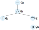
Example 6.2.

Consider the tree automaton defined by states $Q=\{q_{0},q_{1}\}$, $\mathcal{F}_{0}=\{0,1\}$, $\mathcal{F}_{1}=\{\neg\}$ $\mathcal{F}_{2}=\{\land\}$, final state $q_{1}$, and the following transitions $\Delta$:

$$\begin{array}[]{ l l l l }1\rightarrow q_{1}&0\rightarrow q_{0}&\land(q_{0},q_{0})\rightarrow q_{0}&\land(q_{0},q_{1})\rightarrow q_{0}\\ \neg(q_{1})\rightarrow q_{0}&\neg(q_{0})\rightarrow q_{1}&\land(q_{1},q_{0})\rightarrow q_{0}&\land(q_{1},q_{1})\rightarrow q_{1}\\ \end{array}$$

This tree automaton accepts exactly those propositional logic formulas (without variables) that evaluate to true. As an example, Fig. 11 shows the tree for the formula $\neg(1\land\neg 0)$ where each sub-term is annotated with its state. Since $q_{0}$ is not a final state, this formula is rejected by the tree automaton.

6.2. Simple programs as tree automata

Suppose we are given a single input-output example $i\mapsto L$ where we have $i\in\textsf{Cells}(\textsf{T})$ and $L$ is either $\bot$ or a list of cells $[o_{1},\cdot\cdot,o_{t}]$ in table T. Our key idea is to construct a (deterministic) bottom-up FTA $\mathcal{A}$ such that $\mathcal{L}(\mathcal{A})$ represents exactly those simple programs (i.e., abstract syntax trees) that produce output $L$ on input cell $i$.

Before presenting the full FTA construction procedure, we first explain the intuition underlying our automata. At a high level, the alphabet of the FTA corresponds to our DSL constructs, and the states in the FTA represent cells in table T. The constructed FTA contains a transition $f(c_{1},\cdot\cdot,c_{n})\rightarrow c$ if it is possible to get to cell $c$ from cells $c_{1},\cdot\cdot c_{n}$ via the DSL construct $f$. Hence, given an input cell $c$ and output cell $c^{\prime}$, the trees accepted by our FTA correspond to simple programs that produce output cell $c^{\prime}$ from input cell $c$.

$$\begin{array}[]{ c c c c }\mkern-2.0mu\displaystyle\frac{}{\vphantom{,}\lambda c.c\in\textsf{Mappers}(\textsf{T})}\mkern-2.0mu&~{}~{}~{}~{}\mkern-2.0mu\displaystyle\frac{\begin{array}[]{c}1\leq k\leq\textsf{NumCols}(\textsf{T})\\ \end{array}}{\vphantom{,}\lambda c.(k,\textsf{col}(c))\in\textsf{Mappers}(\textsf{T})}\mkern-2.0mu&~{}~{}~{}~{}\mkern-2.0mu\displaystyle\frac{\begin{array}[]{c}1\leq k\leq\textsf{NumRows}(\textsf{T})\\ \end{array}}{\vphantom{,}\lambda c.(\textsf{row}(c),k)\in\textsf{Mappers}(\textsf{T})}\mkern-2.0mu&~{}~{}~{}~{}\mkern-2.0mu\displaystyle\frac{}{\vphantom{,}\textsf{True}\in\textsf{Preds}(\textsf{T})}\mkern-2.0mu\end{array}$$

$$\begin{array}[]{ c c c }\mkern-2.0mu\displaystyle\frac{\begin{array}[]{c}\chi\in\textsf{Mappers}(\textsf{T}),\ \ \triangleleft\in\{=,\neq\}\\ \exists c\in\textsf{Cells}(\textsf{T}).\ \ s=\textsf{Val}(c)\\ \end{array}}{\vphantom{,}(\textsf{Val}({\chi(z)})\triangleleft s)\in\textsf{Preds}(\textsf{T})}\mkern-2.0mu&~{}~{}~{}~{}\mkern-2.0mu\displaystyle\frac{\begin{array}[]{c}\chi\in\textsf{Mappers}(\textsf{T})\\ \end{array}}{\vphantom{,}\textsf{Val}(\chi(y))=\textsf{Val}(\chi(z))\in\textsf{Preds}(\textsf{T})}\mkern-2.0mu&~{}~{}~{}~{}\mkern-2.0mu\displaystyle\frac{\phi_{1}\in\textsf{Preds}(\textsf{T}),\phi_{2}\in\textsf{Preds}(\textsf{T})}{\vphantom{,}\phi_{1}\wedge\phi_{2}\in\textsf{Preds}(\textsf{T})}\mkern-2.0mu\end{array}$$

Figure 12. Rules for constructing the universe of predicates.

With this intuition in mind, let us now consider the FTA construction procedure in more detail. Given a table T, an input cell $i$, a list of output cells $L$ (or $\bot$ in the case of negative examples), and an integer $t$ denoting the number of output cells, we construct a tree automaton $\mathcal{A}=(Q,\mathcal{F},Q_{f},\Delta)$ in the following way:

• The states $Q$ include all cells in table T as well as two special symbols $q_{\bot}$ and $q^{\star}$:

  $$Q=\{q_{c}\ |\ c\in\textsf{Cells}(\textsf{T})\}\cup\{q_{\bot},q^{\star}\}$$

  Here, $q_{\bot}$ denotes any cell that is outside the range of the input table, and $q^{\star}$ indicates we have reached all desired output cells.

• The final states $Q_{f}$ only include the special symbol $q^{\star}$ (i.e., $Q_{f}=\{q^{\star}\}$).

• The alphabet $\mathcal{F}$ is $\mathcal{F}_{0}\cup\mathcal{F}_{1}\cup\mathcal{F}_{3}\cup\mathcal{F}_{t}$ where $\mathcal{F}_{0}=\{x\}$, $\mathcal{F}_{t}=\{\textsf{List}\}$ , and

  $$\mathcal{F}_{3}=\{\textsf{Filter}_{\phi}\ |\ \phi\in\textsf{Preds}(\textsf{T})\}$$

  $$\mathcal{F}_{1}=\left\{\textsf{GetCell}_{\textsf{dir},k,\phi}\ {\Big{|}}\begin{array}[]{c}\ \textsf{dir}\in\{\textsf{u},\textsf{d},\textsf{l},\textsf{r}\}\land k\in[1,3]\cup[-3,-1]\land\ \phi\in\textsf{Preds}(\textsf{T})\end{array}\right\}$$

  In other words, the alphabet of $\mathcal{A}$ consists of the DSL constructs for simple programs. Since Filter and GetCell statements also use predicates, we construct the universe of predicates $\textsf{Preds}(\textsf{T})$ as shown in Fig. 12 and generate a different symbol for each different predicate. Furthermore, since GetCell also takes a direction and position as input, we also instantiate those arguments with concrete values.

• The transitions $\Delta$ of $\mathcal{A}$ are constructed using the inference rules in Fig. 13. The Init rule says that argument $x$ is bound to input cell $i$. The GetCell rule states that $\textsf{GetCell}_{\textsf{dir},k,\phi}(q_{c})$ can be rewritten to $q_{c^{\prime}}$ if we can get to cell $c^{\prime}$ from $c$ using the GetCell construct in the DSL. The List 1 rule says that we can reach the final state $q^{\star}$ if the arguments of List correspond to cells in the output $L$. Finally, the Filter 1 rule states that we can reach the final state $q^{\star}$ from states $q_{c_{1}},q_{c_{2}},q_{c_{3}}$ via $\textsf{Filter}_{\phi}$ if $\textsf{Filter}(c_{1},c_{2},c_{3},\phi)$ yields the output $L$ on input table T. The second variants of the rules (labeled 2) deal with the special case where $L=\bot$ (negative example). For instance, according to the List 2 rule, we can reach the final state $q^{\star}$ if the desired output is $\bot$ and any of the arguments of List is $\bot$.

$$\begin{array}[]{ c c }\vspace{1pt}\begin{array}[]{ c r }\mkern-2.0mu\displaystyle\frac{}{\vphantom{,}\textsf{T},i,L\vdash x\rightarrow q_{i}\in\Delta}\mkern-2.0mu&{\rm(Init)}\\ \\ \\ \mkern-2.0mu\displaystyle\frac{\begin{array}[]{c}c\in\textsf{Cells}(\textsf{T})\cup\{\bot\}\\ \llbracket{\textsf{GetCell}(c,\textsf{dir},k,\lambda y.\lambda z.\phi)}\rrbracket_{\textsf{T}}=c^{\prime}\\ \end{array}}{\vphantom{,}\textsf{T},i,L\vdash\textsf{GetCell}_{\textsf{dir},k,\phi}(q_{c})\rightarrow q_{c^{\prime}}\in\Delta}\mkern-2.0mu&({\rm GetCell})\\ \\ \mkern-2.0mu\displaystyle\frac{\begin{array}[]{c}L=[o_{1},\cdot\cdot,o_{n}]\\ c_{1}\in\textsf{Cells}(\textsf{T}),c_{2}\in\textsf{Cells}(\textsf{T}),c_{3}\in\textsf{Cells}(\textsf{T})\\ \llbracket{\textsf{Filter}(c_{1},c_{2},c_{3},\lambda y.\lambda z.\phi)}\rrbracket_{\textsf{T}}=L\\ \end{array}}{\vphantom{,}\textsf{T},i,L\vdash\textsf{Filter}_{\phi}(q_{c_{1}},q_{c_{2}},q_{c_{3}})\rightarrow q^{\star}\in\Delta}\mkern-2.0mu&({\rm Filter}\ 1)\end{array}&\begin{array}[]{ c r }\mkern-2.0mu\displaystyle\frac{L=[o_{1},\cdot\cdot,o_{n}]}{\vphantom{,}\textsf{T},i,L\vdash\textsf{List}(q_{o_{1}},\cdot\cdot,q_{o_{n}})\rightarrow q^{\star}\in\Delta}\mkern-2.0mu&({\rm List}\ 1)\\ \\ \mkern-2.0mu\displaystyle\frac{\begin{array}[]{c}L=\bot\\ \exists k\in[1,n].\ q_{j_{k}}=q_{\bot}\\ \forall k\in[1,n].\ q_{j_{k}}\neq q^{\star}\end{array}}{\vphantom{,}\textsf{T},i,L\vdash\textsf{List}(q_{j_{1}},\cdot\cdot,q_{j_{n}})\rightarrow q^{\star}\in\Delta}\mkern-2.0mu&({\rm List}\ 2)\\ \\ \mkern-2.0mu\displaystyle\frac{\begin{array}[]{c}L=\bot\\ \exists k\in[1,3].\ q_{j_{k}}=q_{\bot}\\ \forall k\in[1,3].\ q_{j_{k}}\neq q^{\star}\end{array}}{\vphantom{,}\textsf{T},i,L\vdash\textsf{Filter}_{\phi}(q_{j_{1}},q_{j_{2}},q_{j_{3}})\rightarrow q^{\star}\in\Delta}\mkern-2.0mu&({\rm Filter}\ 2)\end{array}\end{array}$$

Figure 13. Rules for constructing transition rules $\Delta$ for table T and example $i\mapsto L$.

Theorem 6.3.

(Soundness and Completeness) Let $\mathcal{A}$ be the finite tree automaton constructed by our technique for example $i\mapsto L$ and table T. Then, $\mathcal{A}$ accepts the tree that represents a simple program $\rho$ iff $\llbracket{\rho}\rrbracket_{\textsf{T},i}=L$.

Proof.

Provided in the appendix. ∎

Tree
Prog.	$\textsf{List}(\textsf{GetCell}(x,\textsf{u},2,\lambda y.\lambda z.\textsf{True}))$	$\textsf{List}(\textsf{GetCell}(x,\textsf{u},1,\lambda y.\lambda z.\textsf{Val}(z)\neq\textnormal{{?}}))$	$\textsf{Filter}\big{(}x,\textsf{GetCell}(x,\textsf{u},-1,\lambda y.\lambda z.\textsf{True}),\textsf{GetCell}(x,$ $~{}~{}~{}~{}~{}~{}~{}~{}~{}~{}~{}~{}\textsf{d},-1,\lambda y.\lambda z.\textsf{True}),\lambda y.\lambda z.\textsf{Val}(z)\neq\textnormal{{?}}\big{)}$
Desc.	The previous cell upwards	The previous non-missing cell upwards	All non-missing cells in the same column

Figure 14. Three terms (programs) accepted by the tree automaton in Example 6.4.

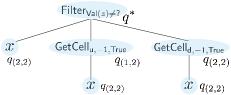
Example 6.4.

Consider a small table with two rows, where the first row is $[4,5]$ and the second row is $[6,\textnormal{{?}}]$. Furthermore, suppose the user provides the sketch $\textnormal{{?}}_{1}$ and the example $\{(2,2)\mapsto[(1,2)]\}$ (i.e., ? should be $5$).

Let us consider the FTA construction for this example. The states in the FTA are $\{q_{(1,1)},q_{(1,2)},q_{(2,1)},q_{(2,2)},q_{\perp},q^{*}\}$, and the final state is $q^{*}$. The transition rules $\Delta$ of the FTA are constructed according to Fig. 13. For example, $\Delta$ includes $x\rightarrow q_{(2,2)}$ because cell $(2,2)$ is the input cell in the example (Init). It also includes $\textsf{GetCell}_{\textsf{u},2,\textsf{True}}(q_{(2,2)})\rightarrow q_{(1,2)}$ because, using GetCell, we have

$$\llbracket{\textsf{GetCell}((2,2),\textsf{u},2,\lambda y.\lambda z.\textsf{True})}\rrbracket_{\textsf{T}}=(1,2)$$

Using List 1, the transition rules $\Delta$ also include the transition $\textsf{List}(q_{(1,2)})\rightarrow q^{*}$ and, using Filter 1, it contains:

$$\textsf{Filter}_{\textsf{Val}(z)\neq\textnormal{{?}}}(q_{(2,2)},q_{(1,2)},q_{(2,2)})\rightarrow q^{*}$$

6.3. Ranking programs accepted by tree automaton

Recall from Section 5 that the LearnSimpProg algorithm requires finding the “best” program accepted by $\mathcal{A}$ according to a Rank function. In this section, we briefly discuss how we rank programs accepted by a tree automaton. In the rest of this section, we use the term “program” and its corresponding AST interchangably.

Definition 6.5.

The size of a tree (term) $t$, denoted by $||t||$, is inductively defined by:
- $||t||=1$ if $t\in\mathcal{F}_{0}$,
- $||t||=1+\Sigma_{i\in\{1,\cdot\cdot,n\}}{||t_{i}||}$ if $\textnormal{Root}(t)\in\mathcal{F}_{n}$, where $t_{i}$ is the $i$-th argument of $t$.

The ranking function $\textsc{Rank}(\mathcal{A})$ selects the best program by finding a tree $t$ in $\mathcal{L}(\mathcal{A})$ such that $||t||$ is minimized. If there are multiple trees with the same size, it selects the one with the highest score according to a heuristic scoring function $\theta$. Intuitively, $\theta$ assigns a positive score to each language construct in our DSL so that a more “general” construct has a higher score. For example, the identity mapper $\lambda c.c$ is assigned a higher score than the other cell mappers, and predicate True has a higher score than other predicates. More details about the heuristic scoring function $\theta$ are provided in the appendix.

Example 6.6.

Fig. 14 shows a subset of the programs accepted by the tree automaton $\mathcal{A}$ from Example 6.4. The first program, $\textsf{List}(x,\textsf{u},2,\lambda y.\lambda z.\textsf{True})$, is selected as the best program, because it is of the minimum size (3), and it only uses the most general predicate True.

7. Implementation

We have implemented the synthesis algorithm proposed in this paper in a tool called DACE, written in Java. While our implementation mostly follows our technical presentation, it performs several additional optimizations. First, our presentation of LearnSimpProg algorithm constructs a separate tree automaton for each example. However, observe that the tree automata for different examples actually have the same set of cells and share a large subset of the transitions. Based on this observation, our implementation constructs a base (incomplete) tree automaton $\mathcal{A}_{B}$ that is shared by all examples and then adds additional transitions to $\mathcal{A}_{B}$ for each individual example. Second, our implementation memoizes results of automaton intersection. Since the top-level synthesis algorithm ends up intersecting the same pair of automata many times, this kind of memoization is useful for improving the efficiency of our synthesis procedure. In addition to these optimizations, our implementation also limits the number of nested GetCell constructs to be at most $4$. We have found this restriction to improve the scalability of automaton intersection without affecting expressiveness in practice.

8. Evaluation

In this section, we present the results of our evaluation on $84$ data completion benchmarks collected from online forums. All experiments are conducted on an Intel Xeon(R) machine with an E5-2630 CPU and 64G of memory.

Benchmarks. To evaluate the proposed synthesis technique , we collected a total of $84$ data completion benchmarks from StackOverflow by searching for posts containing relevant keywords such as “data imputation”, “missing value”, “missing data”, “spreadsheet formula”, and so on. We then manually inspected each post and only retained those benchmarks that are indeed relevant to data completion and that contain at least one example. Among these $84$ benchmarks, $46$ involve data imputation in languages such as R and Python, $32$ perform spreadsheet computation in Excel and Google Sheets, and $6$ involve data completion in relational databases.

Recall that an input to DACE consists of (a) a small example table, (b) a sketch formula, and (c) a mapping from each hole in the sketch to a set of examples of the form $i\mapsto[o_{1},\cdot\cdot,o_{n}]$. As it turns out, most posts contain exactly the type of information that DACE requires: Most questions related to data completion already come with a small example table, a simple formula (or a short description in natural language), and a few examples that show how to instantiate the formula for concrete cells in the table.

We categorize our benchmarks in 21 groups according to their shared functionality. Specifically, as shown in  Fig. 15, benchmarks in the same category typically require the same sketch. For instance, all benchmarks in the first category in Fig. 15 share the sketch $\textnormal{{?}}_{1}$ and require filling the missing value with the previous/next non-missing value (with or without the same key). The column labeled “Formula sketch” shows the concrete sketch for each benchmark category. Observe that most of these sketches are extremely simple to write. In fact, for over 50% of the benchmarks, the user only needs to specify the sketch $\textnormal{{?}}_{1}$, which is equivalent to having no sketch at all. The next column labeled Count indicates the number of benchmarks that belong to the corresponding category, and the column called “Avg. table size” shows the average number of cells in the tables for each category. Finally, the last column labeled “Avg. # examples per hole” shows the average number of examples that the user provides in the original StackOverflow post. Observe that this is not the number of examples that DACE actually requires to successfully perform synthesis, but rather the number of all available examples in the forum post.

Benchmark category description		Formula sketch	Count	Avg. table size	Avg. # examples per hole
1	Fill missing value by previous/next non-missing value with/without same keys.	$\textnormal{{?}}_{1}$	24	24.4	5.3
2	Fill missing value by previous (next) non-missing value with/without same keys if one exists, otherwise use next (previous) non-missing value	$\textnormal{{?}}_{1}$	9	25.6	5.7
3	Replace missing value by the average of previous and next non-missing values.	$\texttt{AVG}(\textnormal{{?}}_{1},\textnormal{{?}}_{2})$	3	12.7	2.3
4	Fill missing value by the average of previous and next non-missing values, but if either one does not exist, fill by the other one.	$\texttt{AVG}(\textnormal{{?}}_{1})$	2	21.5	4
5	Replace missing value by the sum of previous non-missing value (with or without the same key) and a constant.	$\texttt{SUM}(\textnormal{{?}}_{1},c)$	3	31.3	5.7
6	Replace missing value by the average of all non-missing values in the same row/column (with or without same keys).	$\texttt{AVG}(\textnormal{{?}}_{1})$	7	21.7	3.1
7	Replace missing value by the max/min of all non-missing values in the column with the same key.	$\texttt{MAX}(\textnormal{{?}}_{1}),\ \texttt{MIN}(\textnormal{{?}}_{1})$	2	28.0	3
8	Fill missing value by linear interpolation of previous/next non-missing values.	$\texttt{INTERPOLATE}(\textnormal{{?}}_{1},\textnormal{{?}}_{2})$	2	28.0	7.5
9	Fill cells by copying values from other cells in various non-trivial ways, such as by copying the first/last entered entry in the same/previous/next row, and etc.	$\textnormal{{?}}_{1}$	13	44.5	10.2
10	Fill value by the sum of a range of cells in various ways, such as by summing all values to the left with the same keys.	$\texttt{SUM}(\textnormal{{?}}_{1})$	4	47.8	10.3
11	Fill cells with the count of non-empty cells in a range.	$\texttt{COUNT}(\textnormal{{?}}_{1})$	1	32.0	3
12	Fill cells in a column by the sum of values from two other cells.	$\texttt{SUM}(\textnormal{{?}}_{1},\textnormal{{?}}_{2})$	2	38.3	6.5
13	Fill each value in a column by the difference of values in two other cells in different columns found in various ways.	$\texttt{MINUS}(\textnormal{{?}}_{1},\textnormal{{?}}_{2})$	4	39.0	3.5
14	Replace missing value by the average of two non-missing values to the left.	$\texttt{AVG}(\textnormal{{?}}_{1},\textnormal{{?}}_{2})$	1	32.0	5
15	Complete a column so that each value is the difference of the sum of a range of cells and another fixed cell.	$\texttt{MINUS}(\texttt{SUM}(\textnormal{{?}}_{1}),\textnormal{{?}}_{2})$	1	27.0	8
16	Fill each value in a column by the difference of a cell and sum of a range of cells.	$\texttt{MINUS}(\textnormal{{?}}_{1},\texttt{SUM}(\textnormal{{?}}_{2}))$	1	10.0	3
17	Create column where each value is the max of previous five cells in sibling column.	$\texttt{MAX}(\textnormal{{?}}_{1})$	1	60.0	15
18	Fill blank cell in a column by concatenating two values to its right.	$\texttt{CONCAT}(\textnormal{{?}}_{1},\textnormal{{?}}_{2})$	1	12.0	2
19	Fill missing value by the linear extrapolation of the next two non-missing values to the right, but if there is only one or zero such entries, fill by the linear extrapolation of the previous two non-missing values to the left.	$\texttt{EXTRAPOLATE}(\textnormal{{?}}_{1})$	1	121.0	16
20	Replace missing values by applying an equation (provided by the user) to the previous and next non-missing values.	$\texttt{SUM}(\textnormal{{?}}_{1},\frac{\texttt{MINUS}(\textnormal{{?}}_{1},\textnormal{{?}}_{2})}{\texttt{ROW}(\textnormal{{?}}_{2})-\texttt{ROW}(\textnormal{{?}}_{1})})$	1	60.0	9
21	Fill missing value using the highest value or linear interpolation of two values before and after it, based on two different criteria.	—	1	60.0	10
Summary			84	32.0	6.3

Figure 15. Benchmark statistics.

Experimental Setup. Since DACE is meant to be used in an interactive mode where the user iteratively provides more examples, we simulated a realistic usage scenario in the following way: First, for each benchmark, we collected the set $\mathcal{S}$ of all examples provided by the user in the original Stackoverflow post. We then randomly picked a single example $e$ from $\mathcal{S}$ and used DACE to synthesize a program $P$ satisfying $e$. If $P$ failed any of the examples in $\mathcal{S}$, we then randomly sampled a failing test case $e^{\prime}$ from $\mathcal{S}$ and used DACE to synthesize a program that satisfies both $e$ and $e^{\prime}$. We repeated this process of randomly sampling examples from $\mathcal{S}$ until either (a) the synthesized program $P$ satisfies all examples in $\mathcal{S}$, or (b) we exhaust all examples in $\mathcal{S}$, or (c) we reach a time-out of $30$ seconds per synthesis task. At the end of this process, we manually inspected the program $P$ synthesized by DACE and checked whether $P$ conforms to the natural language description provided by the user.

Benchmark category	Count	DACE					PROSE					SKETCH
		# Solved	Running time per benchmark (sec)		# Examples used per hole		# Solved	Running time per benchmark (sec)		# Examples used per hole		# Solved (2 exs)	Running time per benchmark (sec)		# Solved (3 exs)	Running time per benchmark (sec)
			Avg.	Med.	Avg.	Med.		Avg.	Med.	Avg.	Med.		Avg.	Med.		Avg.	Med.
1	24	24	0.41	0.04	1.1	1.0	24	1.32	0.73	1.1	1.0	6	230	224	6	314	281
2	9	9	0.50	0.13	2.7	3.0	7	4.88	1.13	2.4	2.0	2	182	182	0	—	—
3	3	3	0.05	0.04	1.0	1.0	3	5.16	5.89	1.0	1.0	0	—	—	0	—	—
4	2	2	0.19	0.19	2.0	2.0	1	2.11	2.11	2.0	2.0	0	—	—	0	—	—
5	3	3	0.18	0.14	1.3	1.0	3	0.90	0.99	1.7	1.0	0	—	—	0	—	—
6	7	6	0.09	0.07	1.8	2.0	5	15.86	8.31	1.8	2.0	5	353	352	4	399	400
7	2	2	0.66	0.66	2.0	2.0	1	296.17	296.17	3.0	3.0	0	—	—	0	—	—
8	2	2	0.15	0.15	1.0	1.0	1	19.72	19.72	1.0	1.0	1	501	501	0	—	—
9	13	10	1.55	0.31	2.8	2.0	5	6.02	1.52	1.4	1.0	2	507	507	0	—	—
10	4	3	0.42	0.30	1.7	2.0	1	2.27	2.27	2.0	2.0	0	—	—	0	—	—
11	1	1	0.59	0.59	1.0	1.0	0	—	—	—	—	3	223	182	3	353	298
12	2	2	0.51	0.51	1.0	1.0	1	66.95	66.95	2.0	2.0	0	—	—	0	—	—
13	4	4	0.51	0.46	2.0	2.0	2	1.52	1.52	2.0	2.0	0	—	—	0	—	—
14	1	1	0.16	0.16	3.0	3.0	0	—	—	—	—	0	—	—	0	—	—
15	1	1	0.11	0.11	2.0	2.0	1	148.95	148.95	3.0	3.0	0	—	—	0	—	—
16	1	1	0.03	0.03	2.0	2.0	0	—	—	—	—	0	—	—	0	—	—
17	1	1	1.96	1.96	4.0	4.0	1	183.19	183.19	2.0	2.0	1	78	78	1	81	81
18	1	1	0.01	0.01	1.0	1.0	1	1.44	1.44	1.0	1.0	0	—	—	0	—	—
19	1	1	13.66	13.66	5.0	5.0	0	—	—	—	—	0	—	—	0	—	—
20	1	1	1.92	1.92	1.0	1.0	0	—	—	—	—	0	—	—	0	—	—
21	1	0	—	—	—	—	0	—	—	—	—	0	—	—	0	—	—
All	84	78	0.70	0.19	1.8	2.0	57	16.09	1.18	1.5	1.0	20	289	226	14	330	314

Figure 16. Evaluation results of DACE, as well as PROSE and SKETCH as two baselines. The time-out for DACE is set to be $30$ seconds, whereas the time-out for baselines is set to be $10$ minutes.

Results. We present the main results of our evaluation of DACE in Fig. 16. The column “# Solved” shows the number of benchmarks that can be successfully solved by DACE for each benchmark category. Overall, DACE can successfully synthesize over 92% of the benchmarks. Among the six benchmarks that cannot be synthesized by DACE, one benchmark (Category 21) cannot be expressed using our specification language. For the remaining 5 benchmarks, DACE fails to synthesize the correct program due to limitations of our DSL, mainly caused by the restricted vocabulary of predicates. For instance, two benchmarks require capturing the concept “nearest”, which is not expressible by our current predicate language.

Next, let us consider the running time of DACE, which is shown in the column labeled “Running time per benchmark”. We see that DACE is quite fast in general and takes an average of $0.7$ seconds to solve a benchmark. The median time to solve these benchmarks is $0.19$ seconds. In cases where the sketch contains multiple holes, the reported running times include the time to synthesize all holes in the sketch. In more detail, DACE can synthesize 75% of the benchmarks in under one second and 87% of the benchmarks in under three seconds. There is one benchmark (Category 19) where DACE’s running time exceeds $10$ seconds. This is because (a) the size of the example table provided by the user is large in comparison to other example tables, and (b) the table contains over 100 irrelevant strings that form the universe of constants used in predicates. These irrelevant entries cause DACE to consider over $30,000$ predicates to be used in the GetCell and Filter programs.

Finally, let us look at the number of examples used by DACE, as shown in the column labeled “# Examples used per hole”. As we can see, the number of examples used by DACE is much smaller than the total number of examples provided in the benchmark (as shown in Fig. 15). Specifically, while StackOverflow users provide about $6$ examples on average, DACE requires only about $2$ examples to synthesize the correct program. This statistic highlights that DACE can effectively learn general programs from very few input-output examples.

Comparison with PROSE. In this paper, we argued that our proposed FTA-based technique can be viewed as a new version space learning algorithm; hence, we also empirically compare our approach again PROSE (Polozov and Gulwani, 2015), which is the state-of-the-art version space learning framework that has been deployed in Microsoft products. To provide some background, PROSE propagates example-based constraints on subexpressions using the inverse semantics of DSL operators and then represents all programs that are consistent with the examples using a version space algebra (VSA) data structure (Lau et al., 2003).

To allow a fair comparison between PROSE and DACE, we use the same algorithm presented in Section 5 to learn the Seq construct (i.e., branches), but we encode simple programs in the DSL using the PROSE format.  Since PROSE’s learning algorithm requires so-called witness functions, which describe the inverse semantics of each DSL construct, we also manually wrote precise witness functions for all constructs in our DSL. Finally, we use the same scoring function $\theta$ described in the Appendix to rank different programs in the version space.

The results of our evaluation are presented under the PROSE column in Fig. 16. Overall, PROSE can successfully solve 68% of the benchmarks in an average of 15 seconds, whereas DACE can solve 92% of the benchmarks in an average of 0.7 seconds. These results indicate that DACE is superior to PROSE, both in terms of its running time and the number of benchmarks that it can solve. Upon further inspection of the PROSE results, we found that the tasks that can be automated using PROSE tend to be relatively simple ones, where the input table size is very small or the desired program is relatively simple. For benchmarks that have larger tables or involve more complex synthesis tasks (e.g., require the use of Filter operator), PROSE does not scale well – i.e., it might take much longer time than DACE, time out in 10 minutes, or run out of memory. We provide more details and intuition regarding why our FTA-based learning algorithm performs better than PROSE’s VSA-based algorithm in Section 9.

The careful reader may have observed in Fig. 16 that PROSE requires fewer examples on average than DACE (1.5 vs. 1.8). However, this number is quite misleading, as the benchmarks that can be solved using PROSE are relatively simple and therefore require fewer examples on average.

Comparison with SKETCH. Since our synthesis methodology involves a sketching component in addition to examples, we also compare DACE against SKETCH, which is the state-of-the-art tool for program sketching. To compare DACE against SKETCH, we define the DSL operators using nested and recursive structures in SKETCH. For each struct, we define two corresponding functions, namely RunOp and LearnOp. The RunOp function defines the semantics of the operator whereas LearnOp encodes a SKETCH generator that defines the bounded space of all possible expressions in the DSL. The specification is encoded as a sequence of assert statements of the form assert RunExtractor(LearnExtractor(), $i_{k}$) == $L_{k}$, where ($i_{k},L_{k}$) denotes the input-output examples. To optimize the sketch encoding further, we use the input-output examples inside the LearnOp functions, and we also manually unroll and limit the recursion in predicates and cell programs to 3 and 4 respectively.

When we use the complete DSL encoding, SKETCH was able to solve only 1 benchmark out of 84 within a time limit of 10 minutes per benchmark. We then simplified the SKETCH encoding by removing the Seq operator, which allows us to synthesize only conditional-free programs. As shown in Fig. 16, SKETCH terminated on 20 benchmarks within 10 minutes using 2 input-output examples. The average time to solve each benchmark was 289 seconds. However, on manual inspection, we found that most of the synthesized programs were not the desired ones. When we increase the number of input-output examples to 3, 14 benchmarks terminated with an average of 330 seconds, but only 5 of these 14 programs were the desired ones. We believe that SKETCH performs poorly due to two reasons: First, the constraint-based encoding in SKETCH does not scale for complex synthesis tasks that arise in the data completion domain. Second, since it is difficult to encode our domain-specific ranking heuristics using primitive cost operations supported by SKETCH, it often generates undesired programs. In summary, this experiment confirms that a general-purpose program sketching tool is not adequate for automating the kinds of data completion tasks that arise in practice.

9. Version Space Learning using Finite Tree Automata

So far in this paper, we focused on our algorithm for synthesizing data completion tasks in our domain-specific language. However, as argued in Section 1, our FTA-based formulation of unification can be seen as a new version-space learning algorithm. In this section, we outline how our FTA-based learning algorithm could be applied to other settings, and we also discuss the advantages of our learning algorithm compared to prior VSA-based techniques (Lau et al., 2003; Gulwani, 2011; Polozov and Gulwani, 2015).

9.1. The general idea

To see how our FTA-based unification procedure can be used as a general version space learning algorithm, let us consider a domain-specific language specified by a context-free grammar $G=(T,N,P,S)$, where $T$ is a finite set of terminals (i.e., variables and constants), $N$ is the set of non-terminal symbols, $P$ is a set of productions of the form $e\rightarrow F(e_{1},\cdot\cdot,e_{n})$ where $F$ is a built-in DSL function (i.e., “component”), and $S$ is the start symbol representing a complete program. To simplify the presentation, let us assume that the components used in each production are first-order; if they are higher-order, we can combine our proposed methodology with enumerative search (as we did in this paper for dealing with predicates inside the Filter and GetCell constructs).

Now, our general version space learning algorithm works as follows. For each input-output example $\sigma\rightarrow o$, where $\sigma$ is a valuation and $o$ is the output value, we construct an FTA $\mathcal{A}=(Q,\mathcal{F},Q_{f},\Delta)$ that represents exactly the set of programs that are consistent with the examples. Here, the alphabet $\mathcal{F}$ of the FTA consists of the built-in components provided by the DSL.

To construct the states $Q$ of the FTA, let us assume that every non-terminal symbol $n\in N$ has a pre-defined universe $U_{n}=\{v_{1},\cdot\cdot,v_{k}\}$ of values that it can take. Then, we introduce a state $q_{n}^{v_{i}}$ for every $n\in N$ and $v_{i}\in U_{n}$; let us refer to the set of states for all non-terminals in $N$ as $Q_{N}$. We also construct a set of states $Q_{T}$ by introducing a state $q_{t}$ for each terminal $t\in T$. Then, the set of states in the FTA is given by $Q_{N}\cup Q_{T}$.

Next, we construct the transition rules $\Delta$ using the productions $P$ in the grammar. To define the transitions, let us define a function $dom(s)$ that gives the domain of $s$ for every symbol $s$:

$$dom(s)=\left\{\begin{array}[]{ll}s&{\rm if}\ s\ {\rm is\ constant}\\ \sigma(s)&{\rm if}\ s\ {\rm is\ a\ variable}\\ U_{s}&{\rm if}\ s\ {\rm is\ a\ non\text{-}terminal,and\ }U_{s}{\rm\ is\ its\ corresponding\ universe}\\ \end{array}\right.$$

Now, consider a production of the form $n\rightarrow F(s_{1},\cdot\cdot,s_{k})$ in the grammar where $n$ is a non-terminal and each $s_{i}$ is either a terminal or non-terminal. For every $v_{i}\in dom(s_{i})$, we add a transition $F(q_{s_{1}}^{v_{1}},\cdot\cdot,q_{s_{k}}^{v_{k}})\rightarrow q_{n}^{v}$ iff we have $v=\llbracket{F(v_{1},\cdot\cdot,v_{k})}\rrbracket$. In addition, for every variable $x$, we add a transition $x\rightarrow q_{x}$. Finally, the final state $Q_{f}$ is a singleton containing the state $q_{S}^{o}$, where $S$ is the start symbol of the grammar and $o$ is the output in the example.

Given this general methodology for FTA construction, the learning algorithm works by constructing the FTA for each individual example and then intersecting them. The final FTA represents the version space of all programs that are consistent with the examples.

9.2. Comparison with prior version space learning techniques

As mentioned briefly in Section 1, we believe that our FTA-based learning algorithm has two important advantages compared to the VSA-based approach in PROSE. First, FTAs yield a more succinct representation of the version space compared to VSAs in PROSE. To see why, recall that VSA-based approaches construct more complex version spaces by combining smaller version spaces using algebraic operators, such as Join and Union. In essence, PROSE constructs a hierarchy of version spaces where the version spaces at lower levels can be shared by version spaces at higher levels, but cyclic dependencies between version spaces are not allowed. As a result, PROSE must unroll recursive language constructs to introduce new version spaces, but this unrolling leads to a less compact representation with less sharing between version spaces at different layers. The second advantage of our learning algorithm using FTAs is that it does not require complex witness functions that encode inverse semantics of DSL constructs. Specifically, since PROSE propagates examples backwards starting from the output, the developer of the synthesizer must manually specify witness functions. In contrast, the methodology we outlined in Section 9.1 does not require any additional information beyond the grammar and semantics of the DSL.

We refer the interested reader to the Appendix for an example illustrating the differences between PROSE’s VSA-based learning algorithm and our FTA-based technique.

10. Related work

In this section, we compare and contrast our approach with prior work on program synthesis.

Programming-by-example. In recent years, there has been significant interest in programming by example (PBE) (Gulwani, 2011; Polozov and Gulwani, 2015; Wang et al., 2016; Feser et al., 2015; Smith and Albarghouthi, 2016; Osera and Zdancewic, 2015; Bornholt et al., 2016; Udupa et al., 2013; Polikarpova et al., 2016; Yaghmazadeh et al., 2016). Existing PBE techniques can be roughly categorized into two classes, namely enumerative search techniques (Feser et al., 2015; Osera and Zdancewic, 2015; Udupa et al., 2013), and those based on version space learning (Gulwani, 2011; Polozov and Gulwani, 2015; Singh and Gulwani, 2012).

The enumerative techniques search a space of programs to find a single program that is consistent with the examples. Specifically, they enumerate all programs in the language in a certain order and terminate when they find a program that satisfies all examples. Recent techniques in this category employ various pruning methods and heuristics, for instance by using type information (Polikarpova et al., 2016; Osera and Zdancewic, 2015), checking partial program equivalence (Udupa et al., 2013; Albarghouthi et al., 2013), employing deduction (Feser et al., 2015), or performing stochastic search (Schkufza et al., 2013).

In contrast, PBE techniques based on version space learning construct a compact data structure representing all possible programs that are consistent with the examples. The notion of version space was originally introduced by Mitchell (Mitchell, 1982) as a general search technique for learning boolean functions from samples. Lau et al. later extended this concept to version space algebra for learning more complex functions (Lau et al., 2003). The basic idea is to build up a complex version space by composing together version spaces containing simpler functions, thereby representing hypotheses hierarchically (Pardowitz et al., 2007).

The synthesis algorithm proposed in this paper is another technique for performing version space learning – i.e., we build a data structure (namely, finite tree automaton) that represents all consistent hypotheses. However, our approach differs from previous work using version space learning in several key aspects: First, unlike VSA-based techniques that decompose the version space of complex programs into smaller version spaces of simpler programs, we directly construct a tree automaton whose language accepts all consistent programs. Second, our FTA construction is done in a forward manner, rather than by back-propagation as in previous work (Polozov and Gulwani, 2015). Consequently, we believe that our technique results in a more compact representation and enables better automation.

Program sketching. In sketch-based synthesis (Solar-Lezama et al., 2005; Lezama, 2008; Solar-Lezama et al., 2006, 2007), the programmer provides a skeleton of the program with missing expressions (holes). Our approach is similar to program sketching in that we require the user to provide a formula sketch, such as ${\tt SUM}(\textnormal{{?}}_{1},\textnormal{{?}}_{2})$. However, holes in our formula sketches are programs rather than constants. Furthermore, while SKETCH uses a constraint-based counter-example guided inductive synthesis algorithm, DACE uses a combination of finite tree automata and enumerative search. As we show in our experimental evaluation, DACE is significantly more efficient at learning data completion programs compared to SKETCH.

Tree automata. Tree automata were introduced in the late sixties as a generalization of finite word automata (Thatcher and Wright, 1968). Originally, ranked tree automata were used to prove the existence of a decision procedure for weak monadic second-order logic with multiple successors (Thatcher and Wright, 1968). In the early 2000s, unranked tree automata have also gained popularity as a tool for analyzing XML documents where the number of children of a node are not known a priori (Cristau et al., 2005; Martens and Niehren, 2005). More recently, tree automata have found numerous applications in the context of software verification (Abdulla et al., 2008; Kafle and Gallagher, 2015), analysis of XML documents (Hosoya and Pierce, 2003; Cristau et al., 2005; Martens and Niehren, 2005), and natural language processing (May and Knight, 2008; Knight and May, 2009). Most related to our technique is the work of Parthasarathy in which they advocate the use of tree automata as a theoretical basis for synthesizing reactive programs (Madhusudan, 2011). In that work, the user provides a regular $\omega$-specification describing the desired reactive system, and the proposed synthesis methodology constructs a non-deterministic tree automaton representing programs (over a simple imperative language) that meet the user-provided specification. The technique first constructs an automaton that accepts reactive programs corresponding to the negation of the regular $\omega$-specification, and then complements it to obtain the automaton for representing the desired set of programs. In contrast to the purely theoretical work of Parthasarathy in the context of synthesizing reactive programs from regular $\omega$-specifications, we show how finite tree automata can be used in the context of program synthesis from examples. Moreover, we combine this FTA-based approach with enumerative search to automatically synthesize programs for real-world data completion tasks in a functional DSL with higher-order combinators.

11. Conclusions and Future Work

In this paper, we presented a new approach for automating data completion tasks using a combination of program sketching and programming-by-example. Given a formula sketch where holes represent programs and a set of input-output examples for each hole, our technique generates a script that can be used to automate the target data completion task. To solve this problem, we introduced a new domain-specific language that combines relational and spatial reasoning for tabular data and a new synthesis algorithm for generating programs over this DSL. Our synthesis procedure combines enumerative search (for learning conditionals) with a new version-space learning algorithm that uses finite tree automata. We also showed the generality of our FTA-based learning algorithm by explaining how it can be used synthesize programs over any arbitrary DSL specified using a context-free grammar.

We evaluated our proposed synthesis algorithm on 84 data completion tasks collected from StackOverflow and compared our approach with two existing state-of-the-art synthesis tools, namely PROSE and SKETCH. Our experiments demonstrate that DACE is practical enough to automate a large class of data completion tasks and that it significantly outperforms both PROSE and SKETCH in terms of both running time and the number of benchmarks that can be solved.

We are interested in two main directions for future work. First, as discussed in Section 8, there are a few benchmarks for which DACE’s DSL (specifically, predicate language) is not sufficiently expressive. While such benchmarks seem to be relatively rare, we would like to investigate how to enrich the DSL so that all of these tasks can be automated. Second, we would like to apply our new version-learning algorithm using FTAs to other domains beyond data completion. We believe that our new VS-learning algorithm can be quite effective in other domains, such as automating table transformation tasks.

Appendix A: Heuristic Scoring Function

Recall that our synthesis algorithm uses a scoring function $\theta$ to choose between multiple programs that satisfy the input-output examples. The design of the scoring fuction follows the Occam’s razor principle and tries to favor simpler, more general programs over complex ones.

In more detail, our scoring function assign scores to constants, cell mappers, and predicates in our DSL in a way that satisfies the following properties:

• A predicate with mapper $\lambda c.c$ has a higher score than the same predicate with other mappers.

• For predicates containing the same mapper $\chi$, we require that the scoring function satisfies the following constraint:

  $$\theta(\textsf{True})>\theta(\textsf{Val}(\chi(z))=\textnormal{{?}})>\theta(\textsf{Val}(\chi(y))=\textsf{Val}(\chi(z)))>\theta(\textsf{Val}(\chi(z))=s)=\theta(\textsf{Val}(\chi(z))\neq s)$$

• $\theta(\phi_{1},\cdot\cdot,\phi_{n})$ takes into account both the scores of each conjunct as well as the number of conjuncts. That is, $\theta$ assigns a higher score to predicates that have conjuncts with higher scores, and assigns lower scores to predicates with more conjuncts. One design choice satisfying this criterion is to take the average of scores of all the terms in the conjunct.

• For scores of integer $k$ we have $\theta(1)>\theta(2)>\theta(-1)>\theta(3)>\theta(-2)>\theta(-3)$.

Using the scores assigned to predicates, mappers, and constants, we then assign scores to more complex programs in the DSL in the following way. The score of a GetCell program is defined by taking into account both the scores of its arguments and the recursion depth (number of nested GetCell constructs). One possible way to assign scores to GetCell programs is therefore the following:

$$\theta(\textsf{GetCell}(x,\textsf{dir},k,\lambda y\lambda z.\phi)) :=\theta(k)\cdot\theta(\phi)$$

$$\theta(\textsf{GetCell}(\tau,\textsf{dir},k,\lambda y\lambda z.\phi)) :=\frac{\theta(\tau)+\theta(k)\cdot\theta(\phi)}{\textit{depth}(\tau)}$$

$$\textit{depth}(x) :=0$$

$$\textit{depth}(\textsf{GetCell}(\tau,\textsf{dir},k,\lambda y\lambda z.\phi)) :=\textit{depth}(\tau)+1$$

The score of a simple program, i.e., $\textsf{List}(\tau_{1},\cdot\cdot,\tau_{n})$ or $\textsf{Filter}(\tau_{1},\tau_{2},\tau_{3},\lambda y\lambda z.\phi)$, takes into account of the scores of its arguments and the number of the arguments. Specifically, it assigns scores in the following way:

$$\theta(\textsf{List}(\tau_{1},\cdot\cdot,\tau_{n})) :=\frac{\theta(\tau_{1})+\cdot\cdot+\theta(\tau_{n})}{n}$$

$$\theta(\textsf{Filter}(\tau_{1},\tau_{2},\tau_{3},\lambda y\lambda z.\phi)) :=\frac{\theta(\tau_{1})+\theta(\tau_{2})+\theta(\tau_{3})}{3}$$

Appendix B: Proof of Soundness and Completeness

Theorem 11.1.

(Soundness and Completeness) Let $\mathcal{A}$ be the finite tree automaton constructed by our technique for example $i\mapsto L$ and table T. Then, $\mathcal{A}$ accepts the tree that represents a simple program $\rho$ iff $\llbracket{\rho}\rrbracket_{\textsf{T},i}=L$.

Proof.

We first prove soundness – i.e., if $\mathcal{A}$ accepts the tree $t$ that represents a simple program $\rho$, then we have $\llbracket{\rho}\rrbracket_{\textsf{T},i}=L$. We show this by inductively proving (call it $P$) that for any program $p$ whose program tree is a sub-tree $t^{\prime}$ of $t$ and whose height is at most $h$, we have

$$\llbracket{p}\rrbracket_{\textsf{T},i}=\left\{\begin{aligned} &L&\text{if}~{}\text{Root}(t^{\prime})=q^{*}\\ &o&\text{if}~{}\text{Root}(t^{\prime})=q_{o}\\ \end{aligned}\right.$$

The base case for $h=1$ trivially holds, since we have $p=x$, $t=q_{i}$, $t^{\prime}=q_{i}$, and $\llbracket{p}\rrbracket_{\textsf{T},i}=i$. For the inductive case, we want to prove that $P$ holds for any sub-tree $t^{\prime}$ of height $h+1$. Suppose $t^{\prime}=f_{\vec{\omega}}(t^{\prime}_{1},\cdot\cdot,t^{\prime}_{m})$ and consider $t^{\prime}$’s $m$ child-trees $t^{\prime}_{1},\cdot\cdot,t^{\prime}_{m}$. Because a child-tree $t^{\prime}_{j}$ is of height at most $h$, $P$ holds for $t^{\prime}_{j}$ according to the inductive hypothesis. Furthermore, we have

$$\llbracket{f(o_{1},\cdot\cdot,o_{m},\vec{\omega})}\rrbracket=\left\{\begin{aligned} &L&\text{if}~{}\text{Root}(t^{\prime})=q^{*}\\ &o&\text{if}~{}\text{Root}(t^{\prime})=q_{o}\\ \end{aligned}\right.$$

according to the rules in Fig. 13. Therefore, $P$ also holds for any sub-tree $t^{\prime}$ of height $h+1$, and for any sub-tree of height at most $h+1$ as well due to the inductive hypothesis.

Now we turn to the proof of completeness – i.e., if there is a simple program $\rho$ that $\llbracket{\rho}\rrbracket_{\textsf{T},i}=L$, then $\mathcal{A}$ accepts $\rho$’s program tree $t$. Consider the evaluation of $\rho$ given input cell $i$. In each step in which it evaluates a function of the form $f(o_{1},\cdot\cdot,o_{m},\vec{\omega})$ where we have $o_{j}\in\textsf{Cells}(\textsf{T})\cup\{\bot\}$, there exists a transition in $\mathcal{A}$ that goes from states $q_{o_{1}},\cdot\cdot,q_{o_{m}}$ to a state that represents the evaluation result with an $m$-ary function $f_{\vec{\omega}}$ (according to the rules in Fig. 13). Therefore, there exists a tree that is accepted by $\mathcal{A}$ (according to our construction) and represents simple program $\rho$. ∎

Appendix C: Complexity

The complexity of our synthesis algorithm depends on the number of examples $n$, the number of branches $k$ in the target program, and the size of the input table (number of cells), $m$. Specifically, the running time complexity of the algorithm is $\mathcal{O}{(k^{n}\cdot(m^{2})^{n})}$. To see where this result comes from, observe that the worst-case complexity of our FTA construction is $\mathcal{O}{(|\Delta|)}$, where $\Delta$ is the set of transitions. In our case, $|\Delta|$ is bound by $m^{2}$ because we can have a transition for each pair of cells. Since the number of examples is $n$ and FTA intersection takes quadratic time in the size of each FTA, the time to unify $n$ examples is bound by $\mathcal{O}{((m^{2})^{n})}$. Finally, if the learned program has $k$ branches, our algorithm searches for $k^{n}$ possible partitions. Thus, an upper bound on the run-time complexity is $\mathcal{O}{(k^{n}\cdot(m^{2})^{n})}$. However, in practice, since the constructed FTAs are quite sparse, FTA intersection does not result in a quadratic blow-up and remains roughly linear. Hence, in practice, the complexity is closer to $\mathcal{O}{(k^{n}\cdot m^{2})}$. Furthermore, in PBE systems, the user is expected to provide a small number of examples; otherwise, the technique would be too cumbersome for the user. Therefore, in practice, $n$ is expected to be a small number (at most 5 in our experiments). Finally, since the target programs typically do not have a large number of branches, $k$ is also expected to be quite small in practice (at most 3 in our experiments).

Appendix D: In-depth comparison between Version Space Algebras and Finite Tree Automata

Let us consider how PROSE would solve the simple synthesis problem from Example 6.4. For simplicity, let us only consider the DSL shown in Fig. 19. Here, the top-level construct is a cell program $\tau$, which is either the input cell $x$, or a GetCell program whose arguments are chosen from a restricted space. Note that GetCell is recursive, and we assume PROSE allows at most 3 GetCell programs to be nested together.

$\begin{array}[]{lll}\text{Cell prog.}~{}\tau&:=&x~{}~{}|~{}~{}\textsf{GetCell}(\tau,\textsf{dir},k,\lambda y.\lambda z.\textsf{True})~{};\\ \text{Direction}~{}\textsf{dir}&:=&\textsf{u}~{}|~{}\textsf{d}~{}|~{}\textsf{l}~{}|~{}\textsf{r}~{};\\ \text{int}~{}k&:=&-1~{}|~{}1~{};\\ \end{array}$ Figure 17. A simple DSL. $\begin{array}[]{lll}\text{Cell prog.}~{}\tau&:=&x~{}|~{}\textsf{GetCell}(\tau_{1},\textsf{dir},k,\lambda y.\lambda z.\textsf{True})~{};\\ \text{Cell prog.}~{}\tau_{1}&:=&x~{}|~{}\textsf{GetCell}(\tau_{2},\textsf{dir},k,\lambda y.\lambda z.\textsf{True})~{};\\ \text{Cell prog.}~{}\tau_{2}&:=&x~{}|~{}\textsf{GetCell}(x,\textsf{dir},k,\lambda y.\lambda z.\textsf{True})~{};\\ \text{Direction}~{}\textsf{dir}&:=&\textsf{u}~{}|~{}\textsf{d}~{}|~{}\textsf{l}~{}|~{}\textsf{r}~{};\\ \text{int}~{}k&:=&-1~{}|~{}1~{};\\ \end{array}$ Figure 18. The unrolled grammar in PROSE. Figure 19. Part of the VSA in PROSE.

Fig. 19 shows how PROSE constructs the VSA. Conceptually, PROSE first performs backpropagation of examples in the unrolled grammar (shown in Fig. 19). In particular, given examples of an expression $e$ it deduces examples of each argument in $e$ using witness functions. In our case, if $\tau$ is chosen to be a GetCell program, the example $\{(2,2)\mapsto[(1,2)]\}$ is translated into the example for the first argument $\tau_{1}$, which is $\{(2,2)\mapsto[(1,1)]\}\vee\{(2,2)\mapsto[(1,2)]\vee\{(2,2)\mapsto[(2,2)]\}$, since we have $\bigcup_{\textsf{dir},k}\textsf{GetCell}^{-1}((1,2),\textsf{dir},k,\lambda y.\lambda z.\textsf{True})=\{(1,1),(1,2),(2,2)\}$. This is shown in Fig. 19 as the three edges from the first level $\tau$ to the second level $\tau_{1}$, where nodes represent the specifications. PROSE does backpropagation until it reaches the bottom terminals, i.e., $x$ in our case, and constructs the atomic version spaces for terminal symbols. Then it goes upwards to compose existing version spaces using VSA operations. For instance, node $(2,2)\Rightarrow(2,1)$ for $\tau_{2}$ represents a version space that composes smaller spaces using Union operation. As we can see, nodes that represent examples for $\tau$, $\tau_{1}$ and $\tau_{2}$ are duplicated, even though they are unrolled from the same symbol $\tau$ in the original grammar.

Figure 20. Part of the FTA in DACE.

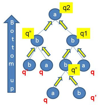
In contrast, our FTA technique does not require unrolling, and thus has the potential to create fewer states and lead to a more compact representation. Fig. 20 shows conceptually how the FTA technique works for the same example. In Fig. 20, nodes represent states in the FTA and edges represent transitions. Our technique starts from the input example, i.e., $(2,2)$, computes the reachable values using the GetCell construct, and creates transitions from the input value to the output values. It does so until all possible transitions are added. As we can see, our technique performs FTA construction in a forward manner, and hence it does not require inverse semantics. Furthermore, it does not require unrolling and results in a more compact FTA representation in this example.

References

- (1)
- Abdulla et al. (2008) Parosh A Abdulla, Ahmed Bouajjani, Lukáš Holík, Lisa Kaati, and Tomáš Vojnar. 2008. Composed bisimulation for tree automata. In International Conference on Implementation and Application of Automata. Springer, 212–222.
- Albarghouthi et al. (2013) Aws Albarghouthi, Sumit Gulwani, and Zachary Kincaid. 2013. Recursive Program Synthesis (CAV). Springer-Verlag, 934–950.
- Alur et al. (2015) Rajeev Alur, Pavol Černỳ, and Arjun Radhakrishna. 2015. Synthesis through unification. In International Conference on Computer Aided Verification. Springer, 163–179.
- Bornholt et al. (2016) James Bornholt, Emina Torlak, Dan Grossman, and Luis Ceze. 2016. Optimizing Synthesis with Metasketches (POPL). ACM, 775–788.
- Comon et al. (2007) H. Comon, M. Dauchet, R. Gilleron, C. Löding, F. Jacquemard, D. Lugiez, S. Tison, and M. Tommasi. 2007. Tree Automata Techniques and Applications. Available on: http://www.grappa.univ-lille3.fr/tata. (2007). release October, 12th 2007.
- Cristau et al. (2005) Julien Cristau, Christof Löding, and Wolfgang Thomas. 2005. Deterministic Automata on Unranked Trees (FCT’05). Springer-Verlag, 68–79.
- Feser et al. (2015) John K. Feser, Swarat Chaudhuri, and Isil Dillig. 2015. Synthesizing Data Structure Transformations from Input-output Examples (PLDI). ACM, 229–239.
- Gulwani (2011) Sumit Gulwani. 2011. Automating String Processing in Spreadsheets Using Input-output Examples (POPL). ACM, 317–330.
- Hosoya and Pierce (2003) Haruo Hosoya and Benjamin C. Pierce. 2003. XDuce: A Statically Typed XML Processing Language. ACM Trans. Internet Technol. 3, 2 (2003), 117–148.
- Kafle and Gallagher (2015) Bishoksan Kafle and John P. Gallagher. 2015. Tree Automata-Based Refinement with Application to Horn Clause Verification (VMCAI 2015). Springer-Verlag New York, Inc., 209–226.
- Knight and May (2009) Kevin Knight and Jonathan May. 2009. Applications of weighted automata in natural language processing. In Handbook of Weighted Automata. Springer, 571–596.
- Lau et al. (2003) Tessa Lau, Steven A. Wolfman, Pedro Domingos, and Daniel S. Weld. 2003. Programming by Demonstration Using Version Space Algebra. Mach. Learn. 53, 1-2 (2003), 111–156.
- Lezama (2008) A Solar Lezama. 2008. Program synthesis by sketching. Ph.D. Dissertation.
- Madhusudan (2011) Parthasarathy Madhusudan. 2011. Synthesizing Reactive Programs. In Computer Science Logic. 428–442.
- Martens and Niehren (2005) Wim Martens and Joachim Niehren. 2005. Minimizing Tree Automata for Unranked Trees. Springer Berlin Heidelberg, 232–246.
- May and Knight (2008) Jonathan May and Kevin Knight. 2008. A Primer on Tree Automata Software for Natural Language Processing. (2008).
- Mitchell (1982) Tom M Mitchell. 1982. Generalization as search. Artificial intelligence 18, 2 (1982), 203–226.
- Osera and Zdancewic (2015) Peter-Michael Osera and Steve Zdancewic. 2015. Type-and-example-directed Program Synthesis (PLDI). ACM, 619–630.
- Pardowitz et al. (2007) Michael Pardowitz, Bernhard Glaser, and Rüdiger Dillmann. 2007. Learning Repetitive Robot Programs from Demonstrations Using Version Space Algebra. In Proceedings of the 13th IASTED International Conference on Robotics and Applications (RA). ACTA Press, 394–399.
- Polikarpova et al. (2016) Nadia Polikarpova, Ivan Kuraj, and Armando Solar-Lezama. 2016. Program Synthesis from Polymorphic Refinement Types (PLDI). ACM, 522–538.
- Polozov and Gulwani (2015) Oleksandr Polozov and Sumit Gulwani. 2015. FlashMeta: A Framework for Inductive Program Synthesis (OOPSLA). ACM, 107–126.
- Schkufza et al. (2013) Eric Schkufza, Rahul Sharma, and Alex Aiken. 2013. Stochastic Superoptimization (ASPLOS ’13). 305–316.
- Singh and Gulwani (2012) Rishabh Singh and Sumit Gulwani. 2012. Synthesizing number transformations from input-output examples (CAV). Springer, 634–651.
- Smith and Albarghouthi (2016) Calvin Smith and Aws Albarghouthi. 2016. MapReduce Program Synthesis (PLDI). ACM, 326–340.
- Solar-Lezama et al. (2007) Armando Solar-Lezama, Gilad Arnold, Liviu Tancau, Rastislav Bodik, Vijay Saraswat, and Sanjit Seshia. 2007. Sketching Stencils (PLDI). ACM, 167–178.
- Solar-Lezama et al. (2005) Armando Solar-Lezama, Rodric Rabbah, Rastislav Bodík, and Kemal Ebcioğlu. 2005. Programming by Sketching for Bit-streaming Programs (PLDI). ACM, 281–294.
- Solar-Lezama et al. (2006) Armando Solar-Lezama, Liviu Tancau, Rastislav Bodik, Sanjit Seshia, and Vijay Saraswat. 2006. Combinatorial Sketching for Finite Programs (ASPLOS). ACM, 404–415.
- Thatcher and Wright (1968) James W Thatcher and Jesse B Wright. 1968. Generalized finite automata theory with an application to a decision problem of second-order logic. Theory of Computing Systems 2, 1 (1968), 57–81.
- Udupa et al. (2013) Abhishek Udupa, Arun Raghavan, Jyotirmoy V. Deshmukh, Sela Mador-Haim, Milo M. K. Martin, and Rajeev Alur. 2013. TRANSIT: specifying protocols with concolic snippets (PLDI). 287–296.
- Wang et al. (2016) Xinyu Wang, Sumit Gulwani, and Rishabh Singh. 2016. FIDEX: Filtering Spreadsheet Data using Examples (OOPSLA). ACM, 195–213.
- Yaghmazadeh et al. (2016) Navid Yaghmazadeh, Christian Klinger, Isil Dillig, and Swarat Chaudhuri. 2016. Synthesizing Transformations on Hierarchically Structured Data (PLDI). ACM, 508–521.