Abstract

We analyse, in NLO, the physical properties of the discrete eigenvalue solution for the BFKL equation. We show that a set of eigenfunctions with positive eigenvalues, $\omega$, together with a small contribution from a continuum of eigenfunctions with negative $\omega$, provide an excellent description of high-precision HERA $F_{2}$ data in the region, $x<0.001$, $Q^{2}>6$ GeV². The phases of the eigenfunctions can be obtained from a simple parametrisation of the pomeron spectrum, which has a natural motivation within BFKL. The data analysis shows that the first eigenfunction decouples completely or almost completely from the proton. This suggests that there exist an additional ground state, which is naturally saturated and may have the properties of the soft pomeron.

Oct 2017

1 Introduction

Figure 1: Evaluation of $F_{2}$ in $\gamma^{*}$ p scattering using the BFKL Green Function

The aim of this paper is to apply, for the first time, the complex BFKL Green Function approach developed in our two previous papers [1, 2] to the analysis of HERA data,. The new approach, although seemingly equivalent to the discrete BFKL solution developed in our previous papers [3, 4], exhibits some differences. The most important of which is that the normalisation of the eigenfunctions is now determined analytically instead of being determined only numerically, as was the case in ref. [3, 4]. As shown in [2], this seemingly minor technical difference has an important consequence: the convergence of the eigenfunctions is now much more rapid than previously. Instead of using O(100) eigenfunctions, as in ref. [3, 4], we need to use only O(10) eigenfunctions to properly represent the Green Function. This constrains substantially the new BFKL solution, exhibits more clearly its physical properties, and leads to new results.

To obtain a good description of the HERA $F_{2}$ data it is necessary to define a non-perturbative boundary condition defined in terms of phases of eigenfunctions at low gluon transverse momenta $k$, close to $k\sim\Lambda_{QCD}$. Since in [3, 4] we were using a large number of eigenfunctions, O(100), it was easy to find a simple, ad hoc, parametrisation for these phases. However, this parametrisation had no physical interpretation.

The first task of this paper is to find a simple parametrisation for the phases of much fewer eigenfunctions, O(10). In the search for such a condition we are guided by the principle of simplicity and some analogy to the Balmer series. In the QCD version of Regge theory developed in our papers, the BFKL equation is considered to be analogous to the Schrödinger equation for the wavefunction of the pomeron. The BFKL kernel corresponds to the Hamiltonian and the eigenvalues $\omega$ to the energy eigenvalues. In this paper, we find that we can specify the boundary condition in terms of a relation between the eigenvalues $\omega_{n}$ of the BFKL operator and the principal quantum number $n$. This relation then determines the boundary condition in terms of the phases $\eta_{n}$ of the eigenfunctions, close to the non-perturbative region, $k\sim\Lambda_{\rm QCD}$. In addition, the relation between $\omega$ and $n$ is very simple and, for large $n$, has a good physical motivation within the context of the BFKL formalism.

We show in this paper that this new approach leads to unexpected results and gives a new insight into the role of gluon density. We recall that the BFKL Green Function is directly related to the gluon density (see below). The properties of this gluon density are very interesting for the LHC and cosmic ray physics. They are also interesting in themselves, because in contrast to the DGLAP evolution [5], the BFKL equation describes a system of quasi-bound self-interacting gluons. Such a system is sensitive to confinement effects and also has some sensitivity to Super-Symmetry effects (in the gluon sector), as was first observed in ref. [3, 4] and is also valid in the present approach.

The paper is organised as follows: In Section 2 we recall the main properties of the BFKL Green Function and of their eigenfunctions, determined in our last papers [1, 2]. We also indicate here the differences between the approach of ref. [3, 4] and our present approach. In Section 3 we introduce the NLO corrections to BFKL and evaluate the properties of eigenvalues and eigenfunctions at NLO. In Section 4 we apply this formalism to HERA data and describe the search for a proper boundary condition and the new results. Finally, in Section 5 we summarise the results and conclude.

2 BFKL Green Function

The Green Function approach considered here is highly appropriate since it does not require any cutoff on the BFKL dynamics and provides a direct relation to the measurements at low-$x$. Thus, the deep inelastic structure function $F_{2}(x,Q^{2})$ can be directly calculated as a convolution of the Green function with impact factors that encode the coupling of the Green function to the external particles that participate in that process.

$$F_{2}(x,Q^{2})\ =\ \int dtdt^{\prime}\Phi_{\gamma}(Q^{2},t){\cal G}(t,t^{\prime},Y)\Phi_{P}(t^{\prime}),$$ (2.1)

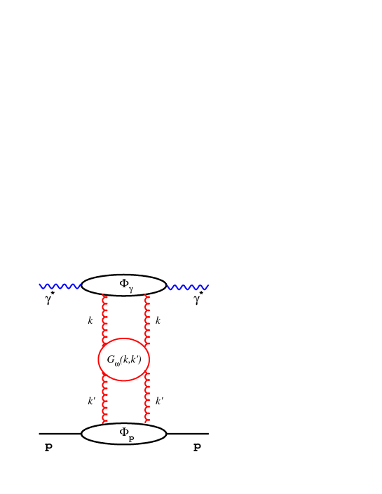
where, $Y=\ln(1/x)$, $t=\ln(k^{2}/\Lambda_{QCD}^{2}),\ t^{\prime}=\ln(k^{\prime\,2}/\Lambda_{QCD}^{2})$; $k,\ k^{\prime}$ being the transverse momenta of the gluons entering the BFKL amplitude. $\Phi_{DIS}(Q^{2},t)$ describes the (perturbativly calculable) coupling of the gluon with transverse momentum $k$ to a photon of virtuality $Q^{2}$ and $\Phi_{P}(t^{\prime})$ describes the coupling of a gluon of transverse momentum $k^{\prime}$ to the target proton, see Fig.1.

In  [1] we determined the BFKL Green Function ${\cal G}_{\omega}(t,t^{\prime})$ (in Mellin space) from the equation

$$\left(\omega-\hat{\Omega}(t,\hat{\nu})\right){\cal G}_{\omega}(t,t^{\prime})\ =\ \delta(t-t^{\prime}),$$ (2.2)

where $\hat{\Omega}$ denotes the BFKL operator, which was given in terms of the LO characteristic function, $\chi(\alpha_{s}(t),\nu)$, by

$$\hat{\Omega}\ =\ \sqrt{\overline{\alpha}_{s}(t)}\left(2\Psi(1)-\Psi\left(\frac{1}{2}+\frac{\partial}{\partial t}\right)-\Psi\left(\frac{1}{2}-\frac{\partial}{\partial t}\right)\right)\sqrt{\overline{\alpha}_{s}(t)},$$ (2.3)

with $\overline{\alpha}_{s}\,\equiv\,C_{A}\alpha_{s}/\pi$. By placing $\sqrt{\overline{\alpha}_{s}(t)}$ on either side of the differential operator we assured the hermiticity of the whole operator.

We have shown in [1, 2] that the Green Function determined in this way has poles on the positive real axis of the $\omega$ plane and a cut along the negative $\omega$ axis. Therefore it can be constructed from the complete set of eigenfunctions of the BFKL operator in the usual way

$${\cal G}(t,t^{\prime},Y)\ =\ \sum_{n=1}^{\infty}x^{-\omega_{n}}f_{\omega_{n}}((t)f^{*}_{\omega_{n}}(t^{\prime})+\lim_{\omega_{min}\to-\infty}\int_{\omega_{min}}^{0}d\omega x^{-\omega}f_{-|\omega|}(t)f_{-|\omega|}(t^{\prime}).$$ (2.4)

The spectrum of the eigenvalues $\omega_{n}$ was found to be discrete for positive values of $\omega$ and continuous for negative value of $\omega$. The complete set of eigenfunctions with positive and negative eigenvalues $\omega$ was found to satisfy the closure relation and the orthonormality condition. In addition, the Green Function converges rapidly so it was sufficient to use only O(10) discrete eigenfunctions (see the discussion below eq.(2.17)) to describe properly the gluon density, as compared to our previous work [3, 4], where we needed more than 100 eigenfunctions.

2.1 Eigenvalues and eigenfunctions

In LO BFKL [14], with fixed QCD coupling constant $\alpha_{S}$, the eigenfunctions have a simple oscillatory behaviour in terms of the gluon transverse variable $t$,

$$f_{\omega}(k)\ \sim\ \exp(\pm i\nu t),$$ (2.5)

The frequency $\nu$ of these oscillations is connected to the eigenvalue $\omega$ by the characteristic equation

$$\omega\ =\overline{\alpha}_{S}\,\chi_{0}(\nu),$$ (2.6)

with

$$\chi_{0}(\nu)\ \equiv\ 2\Psi(1)-\Psi\left(\frac{1}{2}+i\nu\right)-\Psi\left(\frac{1}{2}-i\nu\right).$$ (2.7)

With fixed $\overline{\alpha}_{S}$ the frequency $\nu$ is a one-to-one function of $\omega$. However, when $\alpha_{S}$ is running $\nu$ becomes a function of $t$, $\nu_{\omega}(t)$, in order to compensate the $t$ variation of $\overline{\alpha}_{S}$. For sufficiently large values of $t$ there is no real solution for $\nu_{\omega}(t)$ of eq.(2.6). The transition from the real to imaginary values of $\nu_{\omega}(t)$ singles out a special value of $t=t_{c}$ for which

$$\nu_{\omega}(t_{c})=0.$$ (2.8)

For values of $t$ below the critical point $t_{c}$ the behaviour of the eigenfunction remains oscillatory, but above it becomes exponentially attenuated. This fixes the phase of the eigenfunction at $t=t_{c}$ and together with some fixed non-perturbative phase $\eta_{np}$ leads to quantisation, i.e to a discrete set of eigenfunctions.

To analyse the behaviour of the BFKL equation in the neighbourhood of the turning point, $t_{c}$, it is convenient to define first two related variables, $s_{\omega}(t)$ and $z(t)$. The variable $s_{\omega}(t)$ gives the phase shift from the turning point $t_{c}$ to the point $t$ and corresponds to the argument of the wave function of eq.(2.5). It is defined as

$$s_{\omega}(t)\ =\ \int_{t}^{t_{c}}dt^{\prime}\,\nu_{\omega}(t^{\prime})\,$$ (2.9)

and the ($\omega$ dependent) variable $z(t)$ is defined as

$$z(t)=-\left(\frac{3}{2}s_{\omega}(t)\right)^{\frac{2}{3}}.$$ (2.10)

Using these variables we have shown in [1] that the BFKL operator, $\hat{\Omega}$, can be related to the “generalized Airy operator” as

$$\left(\omega-\hat{\Omega}\left(t,-i\frac{\partial}{\partial t}\right)\right)\ \approx\ \frac{1}{N_{\omega}(t)}\left(\dot{z}z-\frac{\partial}{\partial t}\frac{1}{\dot{z}}\frac{\partial}{\partial t}\right)\frac{1}{N_{\omega}(t)}.$$ (2.11)

In this derivation the diffusion approximation was used in the vicinity of the turning point and the semi-classical approximation far away from it. Using these approximations we have shown [2, 1] that the most general solution to equation 2.11 is given by the Green Function

$${\cal G}_{\omega}(t,t^{\prime})\ =\ \pi N_{\omega}(t)N_{\omega}(t^{\prime})\left[Ai(z(t))\overline{Bi}(z(t^{\prime})\theta(t-t^{\prime})+t\leftrightarrow t^{\prime}\right],$$ (2.12)

with

$$\overline{Bi}(z(t))\ =\ Bi(z(t))+\cot\left(\phi(\omega)\right)Ai(z(t)).$$ (2.13)

Here $Ai(z)$ and $Bi(z)$ denote the two independent Airy functions. The function $\phi(\omega)$ is defined as

$$\phi(\omega)\ =\ s_{\omega}(t_{0})+\frac{\pi}{4}-\eta_{np}(\omega,t_{0})\,$$ (2.14)

with $\eta_{np}(\omega)$ being a non-perturbative phase, fixed at some small $t_{0}$. From 2.12 and 2.13 it follows, as discussed in ref. [1], that the BFKL Green function has poles when

$$\phi(\omega)=n\pi,\ \ n=\ 0,\ 1,\ 2,\ 3\ ...\ .$$ (2.15)

The equations 2.15 and 2.14 define the eigenvalues $\omega_{n}$, which are a function of the non-perturbative boundary condition $\eta_{np}(n)$.

Furthermore, in [1] we have shown that, in case of positive $\omega_{n}$, the eigenfunctions of the BFKL operator are given by

$$f_{\omega_{n}}(t)\ =\ \sqrt{\frac{\pi}{\phi^{\prime}(\omega_{n})}}N_{\omega_{n}}(t)Ai(z(t)),$$ (2.16)

whith $N_{\omega_{n}}(t)$ being the normalisation factor, which is given by

$$N_{\omega_{n}}(t)\ =\ \frac{|z(t)|^{1/4}}{\sqrt{\frac{1}{2}\overline{\alpha}_{s}(t)\chi^{\prime}\left(\nu_{\omega_{n}}(t)\right)}}\ .$$ (2.17)

Here $\chi$ denotes the BFKL characteristic function which in LO is simply equal to $\chi_{0}$ but is more complicated in NLO.

The above expression is similar to the eigenfunctions used in ref. [3, 4] with the difference that the normalisation factor, $N_{\omega_{n}}$, was not $t$ dependent and was determined by numerical integration. In the first paper, in which we developed our new approach [1], we argued that this difference is not very important because the $t$ dependence of the normalisation factor is very slow and would not sizeably change the shape of the eigenfunctions. Whereas this is correct for the shapes in the physical region, it is not true for the normalisation. The numerical integration, which determines the normalisation factor, extends to very large $t$ regions (given by $t_{c}$, see Fig. 3), much above the physical region. Therefore, enhanced $t$ dependence in [3, 4] has a substantial effect when integrated over large $t$ regions. As explained in [2] the eigenfunction of eq.(2.16) converge as $1/n^{2}$, whereas these of ref. [3, 4] converge on a much slower pace, as $1/n$.

To understand the physical meaning of the function $\phi$ it is useful to asymptotically expand the Airy function of eq.(2.16), around $t=t_{0}$ (but far away from $t_{c}$),

$$f_{\omega_{n}}(t_{0})\ \propto\ Ai(z(t_{0}))\ \approx\ \frac{1}{\sqrt{\pi}\ |z(t)|^{1/4}}\sin\left(s_{\omega}(t_{0})+\frac{\pi}{4}\right).$$ (2.18)

This means that the function $\phi$ is the difference between the perturbative and non-perturbative phases of the wave function, which should not depend on $t_{0}$. 

For negative values of $\omega$ eq.(2.8) has no solution, i.e. there is no critical point and no quantization of eigenvalues. The negative $\omega$ eigenfunctions were derived in [2] and are given by

$$f_{-|\omega|}(t)\ =\ \sqrt{\frac{2}{\pi}}\frac{1}{\sqrt{\overline{\alpha}_{s}(t)\chi^{\prime}\left(\nu_{\omega}(t)\right)}}\sin\left(\int_{t_{0}}^{t}\nu_{\omega}(t^{\prime})dt^{\prime}+\eta_{np}\right).$$ (2.19)

The eigenfunctions defined by eq.(2.16) and (2.19) fulfil the completeness relation

$$\lim_{\omega_{min}\to-\infty}\int_{\omega_{min}}^{0}d\omega f_{-|\omega|}(t)f_{-|\omega|}^{*}(t^{\prime})+\sum_{n=1}^{\infty}f_{\omega_{n}}(t)f_{\omega_{n}}(t^{\prime})\ =\ \delta(t-t^{\prime})$$ (2.20)

and are orthonormal, as shown in [2].

3 NLO evaluation

To obtain the eigenfunctions of the BFKL equation in NLO we just need to replace eq.(2.6) by its NLO counterpart

$$\omega\ =\ \overline{\alpha}_{s}\chi_{0}(\nu)+\overline{\alpha}_{s}^{2}\chi_{1}(\nu)+{\cal O}(\overline{\alpha}_{s}^{3})$$ (3.1)

where $\chi_{0}(\nu)$ and $\chi_{1}(\nu)$ are the LO and NLO characteristic functions respectively. The NLO value of $\alpha_{s}$ was fixed by measurement at $Z^{0}$ pole. In our numerical analysis, we modify $\chi_{1}$ following the method of Salam [8] in which the collinear contributions are resummed, leaving a remnant which is accessible to a perturbative analysis. For the analysis of this paper we use Scheme 3 of ref. [8] (see Appendix A).

To create the eigenfunctions we have chosen the value of $t_{0}$ equivalent to $k_{0}=1$ GeV, close to $\Lambda_{QCD}$ but still in the perturbative region, with $\overline{\alpha}_{s}(k_{0})=0.50$. To be able to describe the measured structure function $F_{2}$, which has a changing slope $\lambda$, $\eta_{np}$ should vary with $n$ and the value of the non-perturbative phase $\eta_{np}$ for the leading eigenfunctions should be close to zero (see the discussion in Sections 4.1 and 4.3). We have therefore adopted the convention that $n$ in eq.(2.15) should be counted from 1 and $\eta_{np}$ should be confined to the interval between $+\pi/4$ and $-3\pi/4$. The values of $\eta_{n}$ and the corresponding eigenfunctions, used later in the fit, are not limited to this interval. They are obtained from the periodicity of $\eta_{n}$, i.e. by adding (or subtracting) multiples of $\pi$ on both sides of eq.(2.14). In the following we will label the eigenvalues and eigenfunctions with $n\geq 1$ and denote the $n$ dependent phase $\eta_{np}(n)$ simply by $\eta_{n}$.

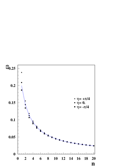
In Fig. 2 we display the eigenvalues $\omega_{n}$ obtained from eq.(3.1), using three different non-perturbative phases, $\eta_{n}=0,\pi/4,-\pi/4$. The dotted line shows, as an example the $\eta_{n}=0$ case, that the dependence of $\omega_{n}$ values from $n$ (for $n>1$) can be simply parametrised by

$$\omega\ =\ \frac{A}{n+B}\ ,$$ (3.2)

as noticed already in [6]. For $\eta_{n}=0$ we found in NLO, that A = 0.52223, B= 1.62001. Since we apply this parametrisation below to describe data we recall its derivation given in ref. [6]. In LO we can integrate $s_{\omega}(t_{0})$ by parts

$$s_{\omega}(t_{0})\ =\ \int_{t_{0}}^{t_{c}}\nu_{\omega}(t^{\prime})dt^{\prime}=-\nu_{\omega}(t_{0})t_{0}+\frac{1}{\bar{\beta_{0}}\omega}\int_{0}^{\nu_{\omega}(t_{0})}\chi_{0}(\nu^{\prime})d\nu^{\prime},$$ (3.3)

where in the last step we used the LO relation $t=\chi_{0}(\nu)/\bar{\beta_{0}}\omega$. For $\omega$ values approaching 0, we have

$$\chi_{0}\left(\nu_{\omega}(t)\right)\ =\ \frac{\omega}{\overline{\alpha}_{s}(t)}\rightarrow 0$$ (3.4)

Therefore, for small $\omega$ and small $t_{0}$, $\nu_{\omega}$ is quickly approaching its asymptotic value, $\nu_{0}$, with $\chi_{0}(\nu_{0})=0$. In this limit $\int_{0}^{\nu_{\omega}(t_{0})}\chi_{0}(\nu^{\prime})d\nu^{\prime}$ and $\nu_{\omega}(t_{0})$ become independent of $\omega$ and eq.(2.14) implies that

$$n\pi\ =a+\frac{b}{\bar{\beta_{0}}\omega}+\frac{\pi}{4}-\eta_{n},$$ (3.5)

where $a,b$ are constants independent of $\omega$. This leads to the relation 3.2. In NLO this relation is satisfied already for $n\geq 2$, since $\nu_{\omega}(t_{0})$ is less dependent on $\omega$ than in LO. The relation 3.2 indicates also that for large $n$, $t_{c}=\chi_{0}(0)/\bar{\beta_{0}}\omega_{n}$ should grow almost linearly with $n$. This is also a feature of the NLO computation, see Fig.3. The value of $t_{c}$ is related to the value of the critical momenta $k_{c}$ by $t_{c}=\ln k_{c}^{2}/\Lambda_{QCD}^{2}$ with $\Lambda_{QCD}=275$ MeV.

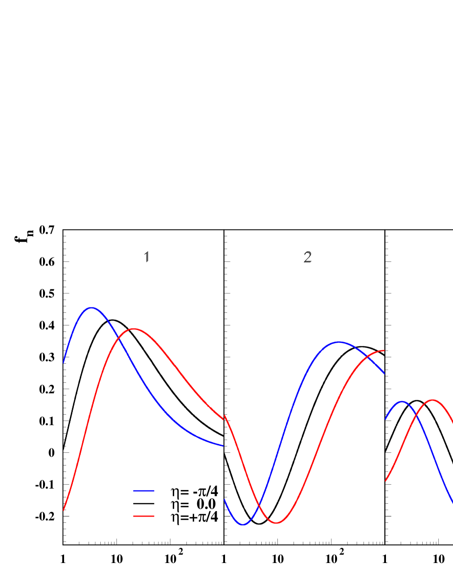
In Fig. 4 we show as example the first three different eigenfunctions 1,2 and 3, computed from eqs.(2.16) and (3.1), at phases $\eta_{n}=0,\pi/4,-\pi/4$.

Figure 2: Eigenvalues $\omega_{n}$ determined in NLO for three fixed non-perturbative phases, $\eta_{n}$. The dotted line shows a simple parametrisation described in the text.

Figure 3: The critical momenta $t_{c}$ determined in NLO for three fixed non-perturbative phases, $\eta_{n}$. $t_{c}=\ln k_{c}^{2}/\Lambda_{QCD}^{2}$ with $\Lambda_{QCD}=275$ MeV.

Figure 4: The first three eigenfunctions computed for three fixed non-perturbative phases, $\eta_{n}$.

4 Application to data

To apply the BFKL Green Function to data, we express the low-$x$ structure function of the proton, $F_{2}(x,Q^{2})$, in terms of the discrete BFKL eigenfunctions by

$$F_{2}(x,Q^{2})\ =\ \int_{x}^{1}d\zeta\int\frac{dk}{k}\Phi_{\gamma}(\zeta,Q,k)xg\left(\frac{x}{\zeta},k\right),$$ (4.1)

where $xg\left(\frac{x}{\zeta},k\right)$ denotes the unintegrated gluon density

$$xg(x,k)\ =\ \int\frac{dk^{\prime}}{k^{\prime}}\Phi_{p}(k^{\prime})\left(\frac{k^{\prime}\,x}{k}\right)^{-\omega_{n}}k^{2}\left(\sum_{n}f^{*}_{\omega_{n}}(k^{\prime})f_{\omega_{n}}(k)+\int_{-\infty}^{0}d\omega x^{-\omega}f_{-|\omega|}(t)f_{-|\omega|}(t^{\prime})\right)$$ (4.2)

and $\Phi_{p}(k)$ denotes the impact factor that describes how proton couples to the BFKL amplitudes at zero momentum transfer. The impact factor, $\Phi_{\gamma}(\zeta,Q,k)$, which describes the coupling of the virtual photon to the eigenfunctions is given in [7]; the dependence on $\zeta$ reflects the fact that beyond the leading logarithm approximation, the longitudinal momentum fraction, $x$, of the gluon differs from the Bjorken-value, determined by $Q^{2}$. $\Phi_{\gamma}(\zeta,Q,k)$ of Ref. [7] is determined taking into account kinematical constraints allowing for non-zero quark masses. The $(k^{\prime}/k)^{\omega_{n}}$ factor arises from a mismatch between the “rapidity”, $Y$, of the forward gluon-gluon scattering amplitude used in the BFKL approach

$$Y\ =\ \ln\left(\frac{s}{kk^{\prime}}\right)$$

and the logarithm of Bjorken $x$, which is given by

$$\ln\left(\frac{1}{x}\right)\ =\ \ln\left(\frac{s}{k^{2}}\right).$$

This ambiguity has no effect in LO but in NLO it can be compensated by replacing the LO characteristic function $\chi_{0}(\nu)$ by $\chi_{0}(\omega/2,\nu)$, which modifies the NLO characteristic function $\chi_{1}$ (see Appendix A).

The proton impact factor is determined by the confining forces. It is therefore barely known, besides the fact that it should be concentrated at the values of $k<{\cal O}(1)$ GeV. We use here a simple parametrisation in the form

$$\Phi_{p}(\mathbf{k})\ =\ A\,k^{2}e^{-bk^{2}},$$ (4.3)

which vanishes as $k^{2}\,\to\,0$, as a consequence of colour transparency and is everywhere positive. The value of $b$ should be around 13 GeV^-2, i.e of the inverse square of $\Lambda_{QCD}=275$ MeV. This is much higher than the value of $b$ determined from data for the proton form factor, $b\approx 4$ GeV^-2. Since the range of the proton impact factor is much smaller than the oscillation period of the BFKL eigenfunctions we do not expect that the results should have substantial sensitivity to a value of $b$. Therefore we performed the investigation assuming two very different values of the impact factor, $b=10$ and $b=20$ GeV^-2, corresponding to $\Lambda_{QCD}\approx 320$ or 220 MeV. We also used, as a check, an extreme proton impact factor, $\Phi_{p}(\mathbf{k})=A\,\delta(k-k_{0})$.

4.1 Properties of HERA data

The HERA $F_{2}$ data in the low $x$ region can be simply parametrised by $F_{2}=c\ (1/x)^{\lambda}$, with the constants $c$ and $\lambda$ being functions of $Q^{2}$, see e.g. [10]. As $Q^{2}$ increases from 4 GeV² to 100 GeV² $\lambda$ changes from about 0.15 to 0.3. The BFKL evaluation of $F_{2}$, which assumes that $\eta_{n}$ is independent of $n$, would predict that $\lambda$ is a constant, $independent$ of $Q^{2}$ with $\lambda\approx\omega_{1}$, since it is the first pole which dominates $F_{2}$, when the value of $\eta_{n}$ is fixed. Therefore, the only way that $\lambda$ can depend on $Q^{2}$ is if the infrared phases, $\eta_{n}$, depend on $n$. Otherwise, the predicted value of $\lambda$ will be about 0.25, $independent$ of $Q^{2}$ (see Fig.2) in clear contradiction with HERA data.

The fits utilize the highest precision HERA data [9] given in terms of reduced cross sections from which we extracted the $F_{2}$ values, using the assumption that $F_{L}$ is proportional to $F_{2}$. We also limit the $y$ range in order to avoid possible complications of a larger contribution from $F_{L}$ (see e.g. [10]). Since we are focusing on the comparison with the $F_{2}$ measurements, we only use the 920 GeV data set of [9]. We also limited the comparison with data to the region $x<0.001$ and $Q^{2}>6$ GeV² since the BFKL equation is valid at very low $x$ only. The $Q^{2}$ cut was chosen to be relatively high to avoid any complications due to possible saturation corrections [11]. The number of experimental points used for fits was then $N_{p}=51$. (It represents around 1/3 of the whole low $x$ data sample, defined as $x<0.01,\ \ Q^{2}>3$ GeV²).

For this investigation we have taken the uncorrelated errors, obtained by adding in quadrature all the correlated errors of ref. [9]. From the data analysis of ref. [11] we know that the uncorrelated errors overestimate the error sizeably, so that the $\chi^{2}/N_{df}$ of a good fit should be around 0.7, instead of about 1 as in case of correlated errors (see also [13]).

4.2 Boundary condition

The major challenge in confronting the BFKL predictions with data is the determination of the infrared boundary condition. i.e. finding the relation between the infrared phases, $\eta_{n}$ and the eigenfunction number $n$ which generates a precise description of the data. At the beginning we tried to parametrise $\eta$ as a function of $n$, using polynomial or other functional dependences. This failed because we were not able to find any functional dependence which would lead to $\chi^{2}<O(500)$. In the next step we tried to find a set of $\eta_{n}$ (with $n=1,2,3...10$) values using only some assumptions of local continuity. This was essentially a 10 parameter fit, with some limitations. After a longer search, using permutational methods to avoid any pre-conceptional bias on the form of $\eta-n$ relation, we found a set of 10 $\eta_{n}$ values which gave an acceptable $\chi^{2}\approx 40$. Studying this set we noticed that it can be well parametrised by an $\omega-n$ relation, similar to eq.(3.2),

$$\omega\ =\ \frac{A}{n+B}+C\ ,$$ (4.4)

with a value of $C$ which is very small, but nevertheless non-zero. The $\eta_{n}$ values were then obtained from eqs.(2.14) and (2.15), by

$$\eta_{n}\ =\ s_{\omega_{n}}(t_{0})+\frac{\pi}{4}-n\pi.$$ (4.5)

The parameters $A$, $B$ and $C$, together with $\eta_{neg}$, the phase of the negative omega contribution, were considered as free parameters of the fit, which we call in the following the ABC-Fit. In addition to these four parameters the overall normalisation was also fitted to data.

As we observed that the system was exhibiting a multitude of local optima, we used the Bayesian Analysis Toolkit (BAT) [12] to find the global optimum. BAT generates samples in parameter space via Markov chain Monte Carlo (MCMC), distributed according to the posterior probability of the parameters. The best fit value is the parameter set with the highest posterior probability, corresponding to the lowest $\chi^{2}$-value. Fig. 5 shows a marginalised distribution of the $ABC$-Fit, for the variables, $B$ and $C$.

Figure 5: Probability density of the $ABC$ fit as a function of the B and C parameters. The legend shows the probability scale in arbitrary units

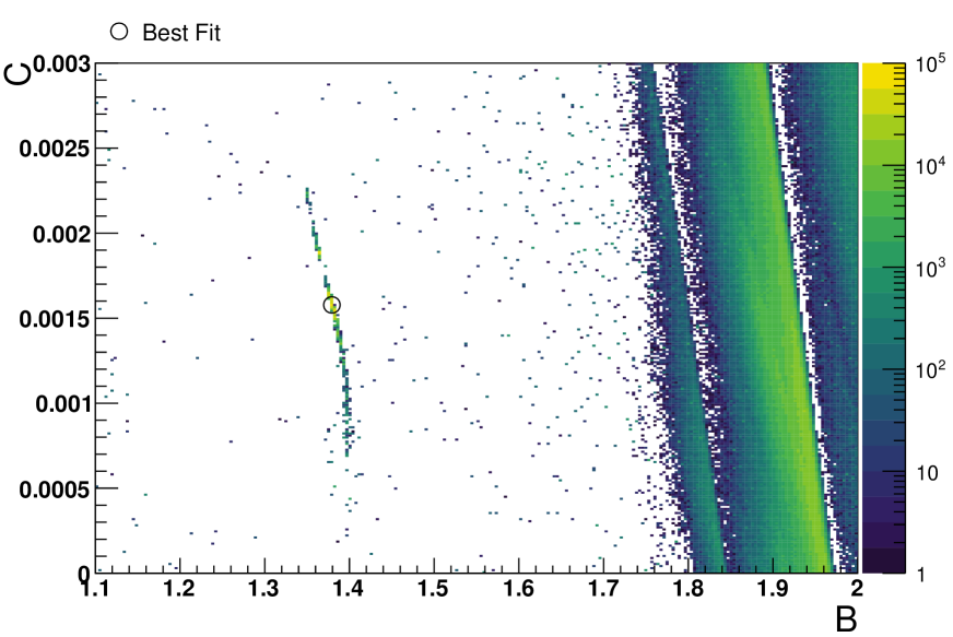
The regions of higher probability are shown as coloured areas, with probability increasing as the colour changes from blue over green to yellow. The small circle shows the position of the best fit, given in Table 1. The complicated structure of the probability distribution is also seen as a function of $A$ and $B$ variables, (see Fig. 6)

Figure 6: Probability density of the $ABC$-Fit as a function of the B and A parameters. The legend shows the probability scale in arbitrary units

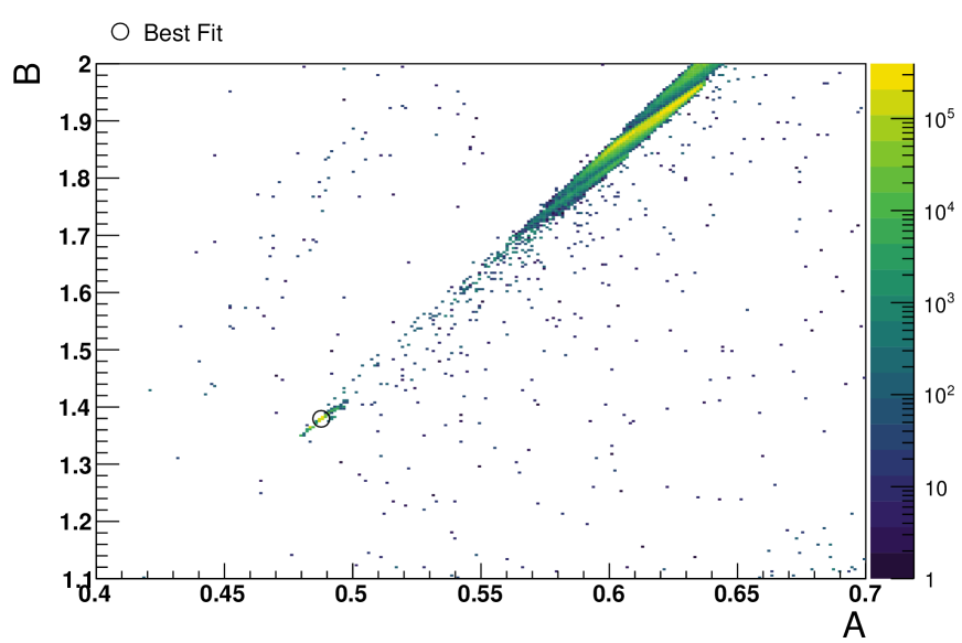
Fig.s 5 and 6 show that the distribution of probability has a complicated structure; there are several extended regions of higher probability, which are completely disconnected. In this situation the usual fitting methods, based on MINUIT, work poorly, since they assume a smooth increase in probability towards the real minimum.

Using the BAT together with the above parametrisation we found an excellent agreement with data, $\chi^{2}/N_{df}\approx 33/46$. We performed this fit for several specific values of the parameters $b$ of $\Phi_{p}$ and found that the $\chi^{2}$ values were the same, within the computational precision of the fit, $\Delta\chi^{2}=\pm 1$. For each value of $b$ the values of the fit parameters, $A,B,C$ and $\eta_{neg}$, were somewhat different and compensated the change of $b$ (see for example Table 1).

$b$ (GeV-2)	10	20
$A$	0.48771	0.47905
$B$	1.37933	1.34020
$C$	0.001578	0.002424
$\eta_{neg}$	-0.0754	-0.0518
$\chi^{2}$	32.9	33.1

Table 1: Results of the ABC-Fit to 51 data points with $x<0.001$ and $Q^{2}>6$ GeV².

The values of the $A$ and $B$ parameters are in the usual range, $A\approx 0.5$, $B\approx 1.5$, similar to the values at fixed phase, $\eta$, (see eq.(3.2) and below). The third parameter, $C$, is very small, O($10^{-3}$), i.e. much smaller than the value of the smallest eigenvalue, $\omega_{20}\approx 0.025$, used in the fit.

In spite of the fact that $C$ is very small, it is impossible to put its value to zero without seriously deteriorating the quality of the $ABC$ fit (to $\chi^{2}\approx 150$). In standard QCD we should expect $C$ to be zero so that $\omega_{n}\rightarrow 0$ when $n\rightarrow\infty$, as in the LO calculation discussed above. However, we noticed, that the parameter $C$ can to be set to zero if we let $\eta_{1}$, the phase of the first eigenfunction, to be a free parameter, instead of $C$. The fits obtained in this way are of the same quality as the $ABC$ fits, they have however an unexpected property; the value of the $\eta_{1}$ parameter is always chosen such that the first eigenfunction decouples (or nearly decouples) from the proton. This means that its overlap with the proton form-factor becomes zero (or nearly zero), independent of the choice of $b$. Therefore, we determined the phase $\eta_{1}$ solely from the requirement that the first eigenfunction should be orthogonal to the proton impact factor (in this way the parameters A and B are correlated, for a given impact factor, with the value of the phase $\eta_{1}$). We call this fit the AB-Fit and give its results in Table 2, for two values of $b$ as example. In the AB-Fit the first eigenfunction is not used since it is decoupling from the proton. In addition, we note that an approximate decoupling happens also in the ABC-Fit, where the contribution of the first pole is much smaller than that of the second one, by more than a factor of 10. Finally we note that in fits of Table 1 and 2 we used 20 eigenfunctions, to see the convergence (see below).

$b$ (GeV-2)	10	20
$A$	0.51844	0.51913
$B$	1.58697	1.58657
$\eta_{neg}$	-0.0911	-0.0550
$\chi^{2}$	33.9	33.3

Table 2: Results of the AB-Fit to 51 data points with $x<0.001$ and $Q^{2}>6$ GeV².

The assumption of the decoupling of the first eigenfunction, together with the AB-relation of eq.(3.2), leads to a much simpler probability structure, (see Fig. 7), with a steady increase of probability towards one minimum, i.e., without a multitude of local minima.

Figure 7: Probability density of the $AB$-Fit as a function of the B and A parameters. The legend shows the probability scale in an arbitrary units

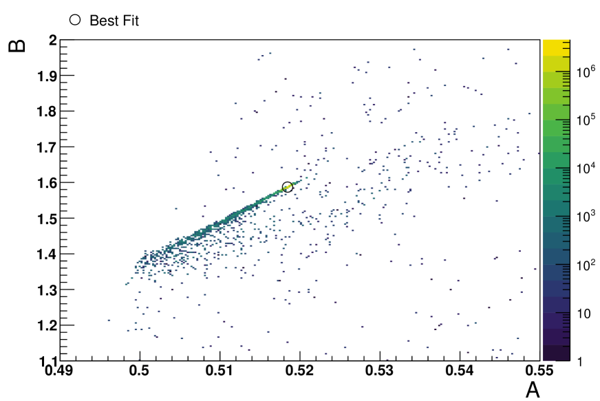
In Fig. 8 we show the $\eta-n$ relation as computed from the parameters $A,B$ of the AB-Fit for two values of $b$. Note that $\eta-n$ relation is visibly different in the two cases, although the parameters $A,B$ differ by a fraction of per mill only. In Fig. 9 we show the same relation as computed from the parameters $A,B,C$ of the ABC-Fit for the same two values of $b$. Note that the $\eta-n$ relation is simpler in the AB-Fit than in the ABC-Fit.

In general, we observe that the AB and ABC parameterisations are characterised by a high sensitivity to the values of $\omega$. The values of the parameters $A,B$ for the case of constant $\eta$, given below eq.(3.2), differ only by about a percent from the values in Table 2, and yet produce a very different $\eta-n$ relation. A fit to data with constant $\eta$ would give $\chi^{2}\approx 3000$!

Figure 8: $\eta-n$ relation as computed from the parameters $A,B$ of the AB-Fit.

Figure 9: $\eta-n$ relation as computed from the parameters $A,B,C$ of the ABC-Fit.

4.3 Fit results

Figure 10: Comparison of the $AB$ fit results with data

Figure 11: Comparison of the $\lambda$ parameter, obtained in the $AB$ fit, with data.

Figure 12: Eigenfunctions 1, 2, 3, and 7, 8 and 9 in the $k$ region accessible to experiments. The eigenfunctions are plotted with the $\eta_{n}$ phases given by the $AB$ fit, performed with the $b$ value of the proton impact factor equal to $10$ GeV^-2 . The first eigenfunction is plotted with the phase which decouples it from the proton.

Figure 13: Eigenfunctions 1, 2, 3, in the $k$ region close to $k_{0}$. The eigenfunctions are plotted with the $\eta_{n}$ phases given by the $AB$ fit. The first eigenfunction is plotted with the phase which gives zero overlap with the proton impact factor. The fits were performed with the $b$-value of the proton impact factor given by $10$ GeV² (full lines) and $20$ GeV² (dotted lines)

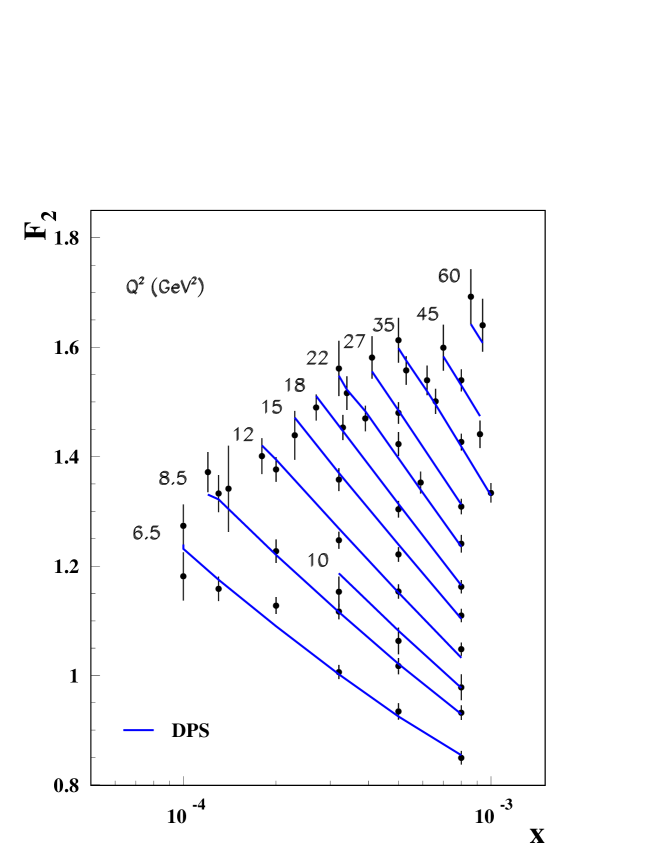
In Fig. 10 we show the comparison of the AB-Fit results with data (with $b=10$ GeV²). Fig. 10 shows a very good agreement, corresponding to the excellent $\chi^{2}$ value. The results obtained with different choices of parameter $b$, or with ABC-Fit, would look the same in this figure.

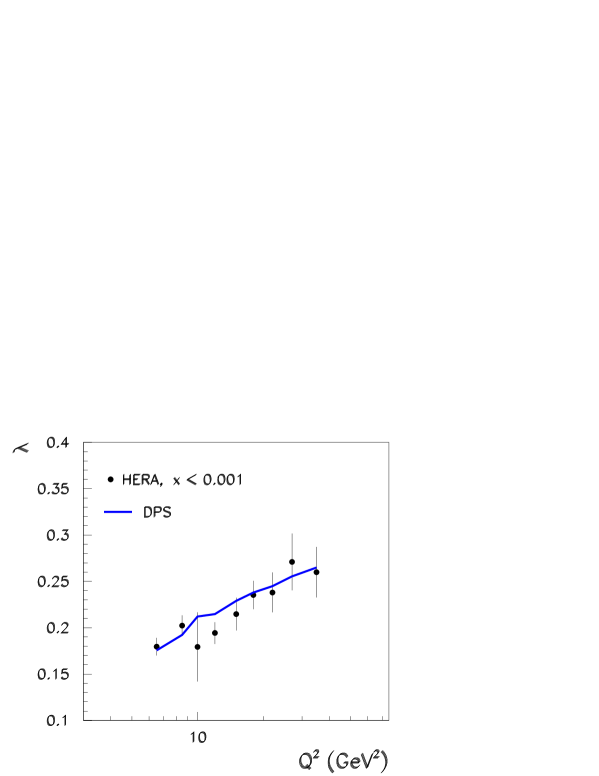
The BFKL Green Function, determined in our approach, is able to describe the $Q^{2}$ dependence of the data, given by the $F_{2}$ values or by the slope $\lambda$, although neither the eigenvalues nor the AB(C)-parameters are $Q^{2}$ dependent. In Fig. 11 we show the comparison of the $\lambda$ parameter obtained from the AB-Fit with data. The $\lambda$ parameter was determined in the very low $x<0.001$ region and in the $Q^{2}$ range between 6.5 and 35 GeV². The $Q^{2}$ dependence enters indirectly because the eigenfunctions depend on the transverse momentum $k$, which in the convolution with the photon impact factor, leads to a $Q^{2}$ dependence .

4.4 Discussion of the phase tuning mechanism

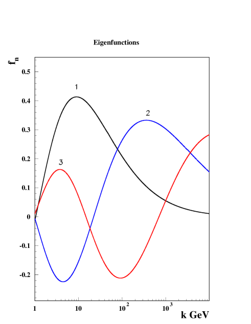
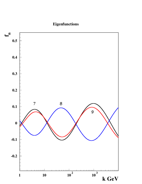
The choice of the $\omega-n$ relation determines the set of phases $\eta_{n}$ which tune the contributions of the individual eigenfunctions to describe the data. To see how this happens we display in Fig. 12 the eigenfunctions 1, 2, 3, and as an example of subleading ones the eigenfunctions 7, 8, 9, as a function of $k$. The eigenfunctions are plotted with the $\eta_{n}$ phases, for $n\geq 2$, given by the AB-Fit. The first eigenfunction has the phase $\eta_{1}$, which suppresses its overlap with the proton impact factor. The figure shows that the leading eigenfunctions 2 and 3 have the values $f_{n}(k_{0})\approx 0$, whereas the eigenfunctions 7, 8 and 9, have the values at $k_{0}$ which are substantially different from zero.

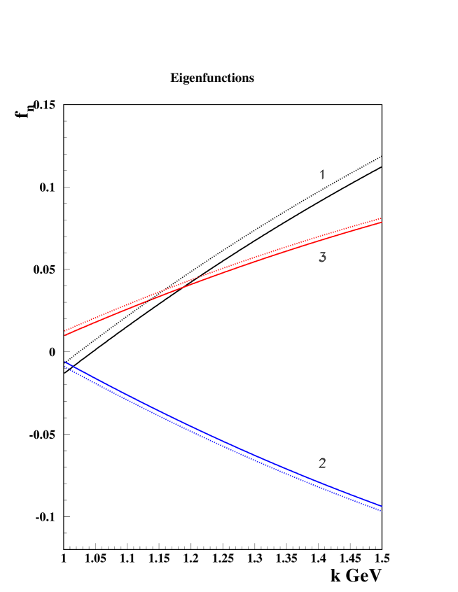
To see more precisely how the phases determine the overlaps, we display in Fig. 13 the eigenfunctions 1, 2 and 3 in the region close to $k_{0}$, for the fits with $b=10$ (full lines) and 20 (dotted lines) GeV². We see that, in both cases, the eigenfunction 1 starts negative at $k_{0}=1$ GeV but then crosses zero at $k_{0}\approx 1.05$ and becomes positive. This small negative region is sufficient to suppress the overlap with the proton impact factor and effectively cancel its contribution to $F_{2}$. The eigenfunction 2 and 3 do not cross zero, and in both cases the overlap with the proton and DIS impact factors have the same signs. They give, therefore, large contributions to $F_{2}$. The contributions of the subleading eigenfunctions 7, 8 and 9 are also significant because $\eta_{n}$ values are substantially different than zero, $\eta_{7}=0.23$, $\eta_{8}=0.32$ and $\eta_{9}=0.42$. This leads to large overlaps with the proton and photon impact factor, but in this case they have have opposite signs. Their contributions to $F_{2}$ are therefore relatively large and have negative sign so that they can generate a $Q^{2}$ dependence in the slope $\lambda$.

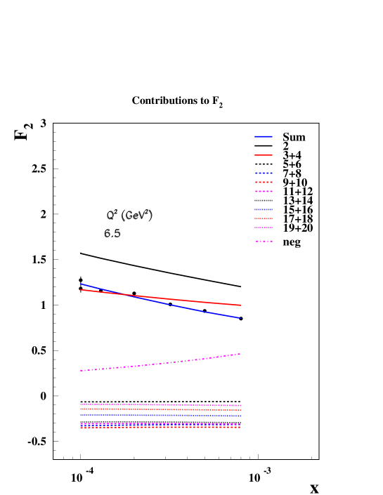
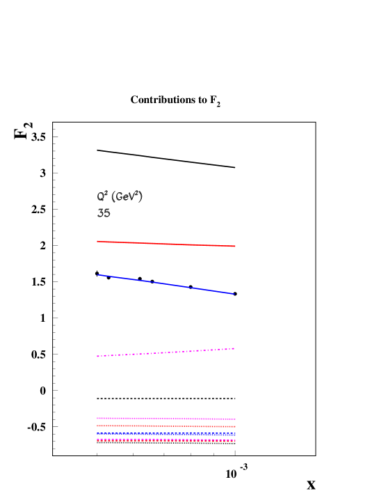
Fig. 14 shows the contributions to $F_{2}$ from individual eigenfunctions, on the samples of results at $Q^{2}=6.5$ and 35 GeV². The larger dots show the measured points, the full blue lines show the BFKL prediction for $F_{2}$, similar to Fig. 10. Other lines show the contributions of eigenfunctions specified in the legend, i.e. the terms

$$F_{2}^{(n)}(x,Q^{2})\ =\ \int_{x}^{1}d\zeta\int\frac{dk}{k}\Phi_{\mathrm{DIS}}(\zeta,Q,k)\int\frac{dk^{\prime}}{k^{\prime}}\Phi_{p}(k^{\prime})\left(\frac{k^{\prime}\,x}{k}\right)^{-\omega_{n}}k^{2}f^{*}_{\omega_{n}}(k^{\prime})f_{\omega_{n}}(k)$$ (4.6)

With exception of the contributions of the second and of the continuous negative $\omega$ terms, the contributions of other eigenfunctions are displayed as a sum of two eigenfunctions, (3+4), (5+6), … (19+20), to simplify the picture. The black full line shows the contribution of the second, leading eigenfunction, which is substantially larger than $F_{2}$.

The contribution of the second eigenfunction, together with the contribution (3+4) and the contribution from the continuum with negative $\omega$, is positive. The contributions of the eigenfunctions 5 to 20 are all negative. The negative contributions correct the positive one to reproduce precisely the measured $F_{2}$. In this way the effective slope is also changed; the contribution of the dominating, second term, which has $\omega_{2}=0.144$, is modified to $\lambda=0.176$ at $Q^{2}=6.5$ GeV² and $\lambda=0.265$ at $Q^{2}=35$ GeV², in agreement with data. Note that the contributions from the subleading eigenfunctions are much larger at $Q^{2}=35$ GeV² than at $Q^{2}=6.5$ GeV² due to the increased overlap with the DIS impact factor. Note also that the variation of the non-perturbative phases leads to a slower convergence of the sub-leading terms than in the case of a constant $\eta$, studied in ref.[2]. This is expected because the contribution of the subleading terms has to be large enough to substantially correct the leading terms in order to reproduce the data. Nevertheless, we see from Fig. 14 that the contributions of eigenfunctions with $n>16$ start to approach zero., i.e. show convergence.

Figure 14: Contributions to $F_{2}$ of individual eigenfunctions. The dots show the measured points at $Q^{2}=6.5$ and 35 GeV², The full blue line shows the BFKL prediction at these $Q^{2}$’s, other lines show the contributions of eigenfunctions specified in the legend. With exception of the second eigenfunction and the continuous negative $\omega$ contributions, the contributions of the eigenfunctions are displayed as a sum of two eigenfunctions, (3+4), (5+6), … (19+20).

Summarising we can confirm that an excellent description of data is achieved by a fine tune of the non-perturbative phases $\eta_{n}$. This phase tune is a result of a simple $\omega-n$ relation which is well motivated in BFKL and is determined by only two or three parameters.

4.5 Decoupling of the first eigenfunction and its consequences

The decoupling or near decoupling of the first eigenfunction is an unexpected and puzzling feature of this investigation. The decoupling is not connected to a particular value of the proton impact factor or to its form. The fits of Tables 1 and 2 together with the example of Fig. 13 show that when we substantially change the value of the proton impact factor, from $b=10$ GeV² to $b=20$ GeV², the values of the fit parameters are re-tuned such that the resulting phases, although sightly changed, reproduce the data very well and again lead to the decoupling of the leading eigenfunction. Note, that these re-tunes hardly change the physical properties of the solution, i.e. the position of the poles, owing to the interplay between the phases eigenfunctions and the parameters AB(C). A similar result is obtained when we choose a completely different impact factor, given by a delta function, $\Phi_{p}=A\,\delta(k-k_{0})$. Although this is not a realistic impact factor, the results are similar; the fit selects the phase of the first eigenfunction such that $f_{\omega_{1}}(k_{0})=0$. The other parameters are re-tuned so that the fit reproduce the data with a $\chi^{2}$ value close to 33, as in the fits of Tables 1 and 2.

From the technical point of view this decoupling occurs because the position of the critical point of the first eigenfunction is relatively close to the physical region, $k_{c}(1)\approx 50$ GeV, whereas the critical point of the subsequent eigenfunctions is far away from it, $k_{c}(2)\approx 3,3$ TeV, $k_{c}(3)\approx 270$ TeV, $k_{c}(4)\approx 20000$ TeV, etc. Therefore, the first eigenfunction varies more quickly near $k_{0}$ than the subsequent ones, so that a very small change in the phase, $\eta_{1}$, leads to a large change of the first contribution.

We have also checked that the results do not depend on the number of eigenfunction used in the fit, provided this number exceeds 10. In Table 3 we show the results of fits made with the first 20, 16, 12 and 10 eigenfunctions. All the fits were made with the ABC relation and in all cases the fit has chosen a phase which decouples the first eigenfunction from the proton.

$N_{ef}$	20	16	12	10
$A$	0.51768	0.47904	0.44987	0.42753
$B$	1.58209	1.32672	1.16597	1.95858
$C$	0.000037	0.002092	0.00431	0.00586
$\eta_{neg}$	-0.0895	-0.0723	-0.0738	-0.0770
$\chi^{2}$	33.4	34.0	34.4	34.7

Table 3: Results of the ABC-Fit performed with different number of eigenfunctions, $N_{ef}$. All fits were using the same 51 data points, with $x<0.001$ and $Q^{2}>6$ GeV². The value of the proton impact factor was $b=10$ GeV².

We conclude therefore that the decoupling or near decoupling of the first eigenfunction is a genuine property of this analysis, independent of the choice of the proton impact factor or the number of eigenfunctions used in the fit.

It is obvious, that this decoupling can only happen because the leading eigenfunction makes a transition from the negative to positive values in a region close to the starting point $k_{0}$. Such a transition is an indication that the first eigenfunction, as chosen by the fit, cannot be a wave function of a ground state because the ground state has to be completely positive, see Appendix B. Therefore, the decoupling of the first eigenfunction should be interpreted as an indication that there exist an additional ground state, corresponding to $n=0$.

Our computation gives us some hints about the properties of such a state. From the values of the turning points, $t_{c}(n)$, which grows almost linearly with $n$, Fig. 3, we can estimate the $k_{c}$ value of the ground state, $n=0$, as being around 700 MeV , just below our starting value of $k_{0}=1$ GeV. Such a state would have a high intercept, $\omega_{0}\approx 0.3$, and would not have any oscillations above $k_{0}$, it would just decay exponentially with increasing $\ln(k)$.

As example of such a state we show in Fig.15 the momentum distribution of a state which could be similar to the real ground state and which exists in our computation. It has $k_{c}=1.05$ GeV, $\omega=0.37$ and $\eta=-2.35$.

Figure 15: Momentum distribution of a state similar to the real ground state, with $k_{c}=1.05$ GeV, $\omega=0.37$ and $\eta=-2.35$.

Indeed, the $k_{c}$ value of the additional ground state, of around 700 MeV, lays right in the middle of the saturation region [16, 17, 18, 19, 20, 21, 22, 23], where multiple pomeron exchanges should dominate [24]. In our approach, these exchanges would almost entirely involve the interaction of the low $k_{c}$ ground state with itself, since its size is much larger than the size of higher eigenfunctions and the eigenfunctions are orthogonal to each other. This will lead to unitarisation (saturation) corrections which would substantially affect the properties of the ground state. The momentum distribution will be shifted towards the lower $k$ values and therefore its overlap with the photon impact factor should diminish quickly with increasing $Q^{2}$. In addition, the saturation correction will damp the effective exponent of the first eigenfunction, $\omega\approx 0.3$, to a value which is compatible with the non-perturbative pomeron state, $\lambda\approx 0.1$.

It was already pointed out by Gribov [15], in the framework of the reggeon calculus, that the soft pomeron could be given by the renormalised, bare pomeron. The renormalisation procedure should take into account the corrections due to multiple interactions. This is somewhat similar to the picture emerging from our analysis. Of course, the soft pomeron discussed by Gribov, was essentially a non-perturbative state, determined mostly by nuclear forces. In our case, the bare ground state is, however, a perturbative state and its multiple interaction are also of perturbative origin. Its properties are thought determined, to large extent, by the non-perturbative, nuclear forces which enter into our analysis through the choice of the non-perturbative phase $\eta$.

4.6 $Q^{2}$ dependence

In Table 4 we show the AB-Fit results for different $Q^{2}$ regions, $Q^{2}>4,\ 6$ and 9 GeV², for $b=10$ GeV^-2 as an example. The fits with $b=20$ GeV² and/or the $ABC$ fits show very similar results.

$Q^{2}$ cut (GeV2)	4	6	9
$A$	0.51852	0.51844	0.51818
$B$	1.58847	1.58697	1.58356
$\eta_{neg}$	-0.0911	-0.0911	-0.0911
$N_{p}$	59	51	37
$\chi^{2}$	68.5	33.9	17.4
$\chi^{2}/N_{df}$	1.25	0.72	0,52

Table 4: Results of the AB-Fit with $x<0.001$ and $b=10$ GeV^-2.

The fit with $Q^{2}>4$ GeV² of Table 4 has a substantially lower quality than the one with $Q^{2}>6$ GeV². Also the fit with $Q^{2}>6$ GeV² is significantly worse than the $Q^{2}>9$ GeV² one. Therefore, it is possible that the worsening of the fit quality with decreasing $Q^{2}$ cut is due to the presence of the hypothetical ground state discussed above.

4.7 Extrapolation to very low $x$

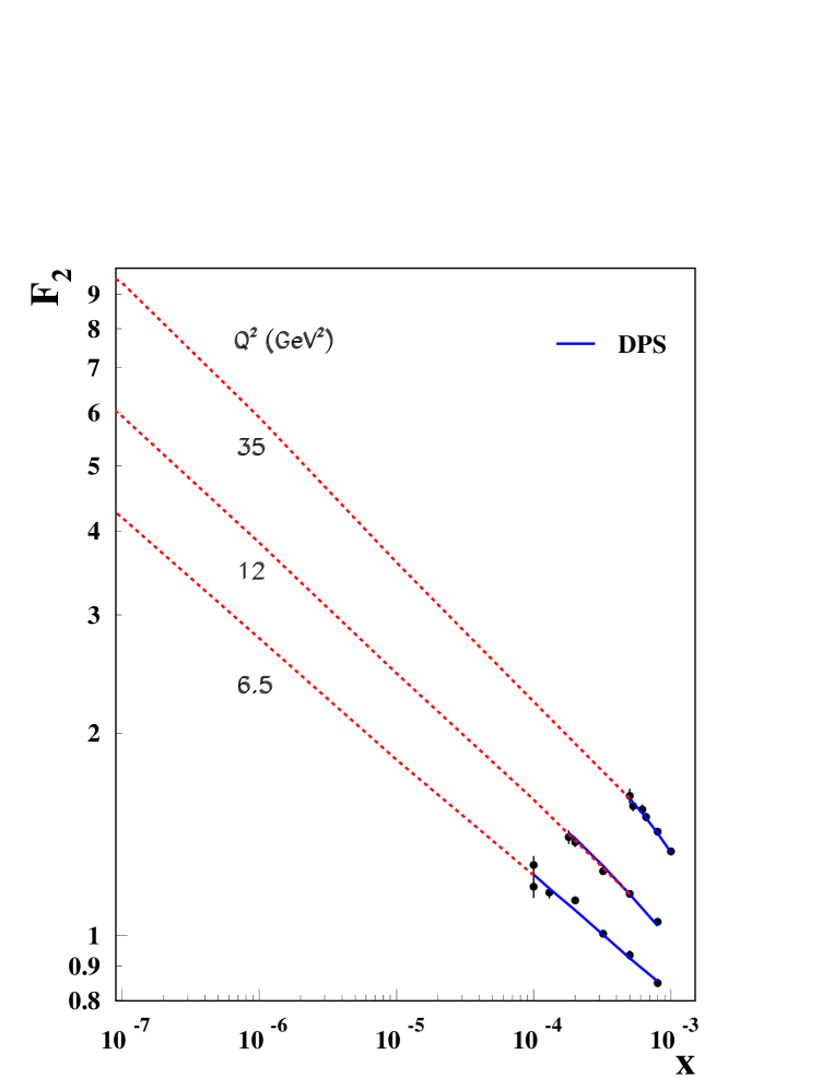
In Fig. 16 we show the extrapolation of the $AB$ fit to very low $x$ values, which can be possibly achieved in some future $ep$ collider like VHEeP or LHeC. We see that at very large energies the increase of $F_{2}$ shows similar slopes at different $Q^{2}$ values, unlike at HERA. This is due to the dominance of the leading trajectory at very low $x$ values.

Figure 16: Extrapolation of the AB fit results to very low $x$

5 Conclusions and Outlook

We have shown here that there exists an infrared boundary condition, which leads to a precise description of HERA $F_{2}$ data, for $x<0.001$. We formulated it in terms of a relation between the eigenvalues, $\omega_{n}$, and the eigenfunction number, $n$. It has a simple form $\omega_{n}=A/(B+n)$ or $\omega_{n}=A/(B+n)+C$, called here $AB$ or $ABC$ relations respectively. Both relations are well motivated in BFKL, for larger $n$. The $\omega-n$ relation determines, within the BFKL Green Function solution, the values of the phases of the eigenfunctions, $\eta_{n}$, close to the non-perturbative region, at small $k\sim\Lambda_{\rm QCD}$. The fits using both relations give an excellent description of data with similar $\chi^{2}$ values.

The fits lead to the unexpected result that the first eigenfunction decouples or nearly decouples. This means that the overlap of the first eigenfunction with the proton impact factor is very small or even zero, due to the fact that the first eigenfunction has a transition region from negative to positive values, i.e. a node. Therefore, the first eigenfunction chosen by the fit cannot be a ground state. This suggests, as a consequence, the existence of a multiply interacting ground state which may have properties of the soft pomeron. The contributions of such a state would be rapidly attenuated as $Q^{2}$ increases. However, at low $Q^{2}$, it should dominate the $F_{2}$ and diffractive processes. A particularly good place to study its effects should be the exclusive diffractive vector meson production, $\rho$, $\phi$ and $J/\psi$, because in this reaction the value of the Regge slope, $\alpha^{\prime}$, is also measured. We may try to learn more about it in our forthcoming paper by focusing the investigation on the region closer to $\Lambda_{QCD}$, by varying $k_{0}$ and, last but not least, using the complete information concerning the errors of HERA data [13].

The present BFKL fits to HERA data predict that in the very low $x$ region, $x<<10^{-4}$, $Q^{2}>6$ GeV², $F_{2}$ should grow with a slope $\lambda$ which is close to the eigenvalue of the second eigenfunction and which is $Q^{2}$ independent. This prediction is possible because there is no interference between the ground state and the second eigenfunction, since they are orthogonal to each other and have very different support. The $\omega$ value of the second eigenfunction could be easily measured on some future $ep$ collider, such as VHEeP [26] or LHeC [25].

Finally, let us note that the AB(C) fits, should be affected by supersymmetry or other physics beyond the standard model (BSM), as discussed in our previous papers [3, 4]. This is because (at least at LO) the constant $A$ is proportional to the beta function, which changes its value drastically once the threshold for the production of gluimos or other BSM particles is crossed. The decoupling of the leading eigenfunctions makes the analysis of BSM physics simpler, especially on the future VHeP or LHeC colliders. This is because the ground state is now very well constrained, the value of the $\omega_{2}$ can be directly measured, and the values of the higher intercepts, $\omega_{n>2}$, can be parametrised reliably.

6 Appendix A

We rephrase here the original derivation of the BFKL resummation given in ref. [8]. It is convenient to write

$$\chi_{0}(\nu)\ \equiv\chi(0,\nu)$$

where

$$\chi(a,\nu)\ \equiv\ 2\Psi(1)-\Psi\left(\frac{1}{2}+a+i\nu\right)-\Psi\left(\frac{1}{2}+a-i\nu\right)$$ (6.1)

and

$$\dot{\chi}(a,\nu)\equiv\ \frac{d}{da}\chi(a,\nu)\ =\ -\Psi^{\prime}\left(\frac{1}{2}+a+i\nu\right)-\Psi^{\prime}\left(\frac{1}{2}+a-i\nu\right)$$ (6.2)

If $a$ is small then up to order $a$ we have

$$\chi(a,\nu)\ =\ \chi(0,\nu)+a\dot{\chi}(0,\nu)+{\cal O}\left(a^{2}\right),$$ (6.3)

We may write $\chi_{1}(\nu)$ (defining a quantity $\chi_{1}^{reg}(\nu)$ ) as

$$\chi_{1}(\nu)\ \equiv\ -A\chi(0,\nu)+B\dot{\chi}(0,\nu)+\frac{1}{2}\chi(0,\nu)\dot{\chi}(0,\nu)+\chi_{1}^{reg}(\nu)$$ (6.4)

By a suitable choice of the constants $A$ and $B$, we can arrange for $\chi_{1}^{reg}(\nu)$ to be free of singularities as $\nu\,\to\pm\frac{i}{2}$.

In this limit we have

$$\chi(0,\nu)\stackrel{{\scriptstyle\nu\to\pm i/2}}{{\longrightarrow}}\frac{1}{\left(\frac{1}{2}\pm i\nu\right)}+{\cal O}\left(\frac{1}{2}\pm i\nu\right)$$ (6.5)

and

$$\dot{\chi}(0,\nu)\stackrel{{\scriptstyle\nu\to\pm i/2}}{{\longrightarrow}}-\frac{1}{\left(\frac{1}{2}\pm i\nu\right)^{2}}+\frac{\pi^{2}}{3}+{\cal O}\left(\frac{1}{2}\pm i\nu\right)$$ (6.6)

So that

$$\chi_{1}(\nu)\stackrel{{\scriptstyle\nu\to\pm i/2}}{{\longrightarrow}}-\frac{1}{2\left(\frac{1}{2}\pm i\nu\right)^{3}}-\frac{B}{\left(\frac{1}{2}\pm i\nu\right)^{2}}-\left(A+\frac{\pi^{2}}{6}\right)\frac{1}{\left(\frac{1}{2}\pm i\nu\right)}$$ (6.7)

Therefore the constants $A$ and $B$ are selected to match the single and double poles respectively of the function $\chi_{1}(\nu)$ and in that way $\chi_{1}^{reg}$ is free from such singularities.

in ref,[8] it is pointed out that the correction due to $\chi_{1}^{reg}$ is genuinely negligible and the entire large correction to the characteristic function come from the terms which are singular as $\nu\to\pm i/2$.

Now let us consider another function $\tilde{\omega}(\nu)$ which is defined as the solution to the transcendental (implicit) equation

$$\tilde{\omega}(\nu)\ \equiv\overline{\alpha}_{s}(1-\overline{\alpha}_{s}A)\chi\left(\frac{\tilde{\omega}}{2}+\overline{\alpha}_{s}B,\nu\right)+\overline{\alpha}_{s}^{2}\chi_{1}^{reg}(\nu)$$ (6.8)

Solving to leading order in $\overline{\alpha}_{s}$ we have

$$\tilde{\omega}\ =\ \overline{\alpha}_{s}\chi(0,\nu)+{\cal O}\left(\overline{\alpha}_{s}^{2})\right).$$ (6.9)

Expanding $\tilde{\omega}(\nu)$ up to order $\overline{\alpha}_{s}^{2}$, and using (6.3) we obtain

$$\tilde{\omega}(\nu) = \overline{\alpha}_{s}(\chi(0,\nu)\ +\ \overline{\alpha}_{s}^{2}\left[-A\chi(0,\nu)+B\dot{\chi}(0,\nu)+\frac{1}{2}\chi(0,\nu)\dot{\chi}(0,\nu)+\chi_{1}^{reg}(\nu)\right]+{\cal O}\left(\overline{\alpha}_{s}^{3}\right)$$ (6.10)

$$= \overline{\alpha}_{s}(\chi_{0}(\nu)+\overline{\alpha}_{s}^{2}\chi_{1}(\nu)+{\cal O}\left(\overline{\alpha}_{s}^{3}\right)$$

Thus we see that up to order $\overline{\alpha}_{s}^{2}$, the quantities $\omega(\nu)$ and $\tilde{\omega}(\nu)$ are identical so that up to that accuracy we may replace the usual perturbative expression given in (3.1) by $\tilde{\omega}(\nu)$.

On the other hand, the quantity $\tilde{\omega}(\nu)$ does not contain any singularities as $\nu\,\to\,\pm\frac{i}{2}$. The singularities we see in eq(6.10) are only present as a result of an expansion. They are therefore an artifact of this expansion and are not present for the entire function. Since it is these singular terms that give rise to the large NLO corrections found in $\chi_{1}(\nu)$ we may consider the quantity $\tilde{\omega}(\nu)$ to be the expression in which all of these large corrections have been resummed.

For the case of the third order pole, this has been established exactly, since we know what the origin of the triple pole is. In rev[8] it is explained that this arises from a mismatch between the “rapidity”, $Y$, of the forward gluon-gluon scattering amplitude used in the BFKL approach

$$Y\ =\ \ln\left(\frac{s}{kk^{\prime}}\right)$$

For the resummation of the double and single poles, this is not known uniquely and there are an infinit enumber of possible resummation schemes, of which one is described here, and three oithers are discusswd in ref.[8]. All these reummation schemes have in common the fact that they resum all the collinear singularities (i.e. all poles as $\nu\,\to\,\pm\frac{i}{2}$ and they are all equivalent to the ordinary pertubative expansion for $\omega$ up to order $\overline{\alpha}_{s}^{2}$. They, of course, differ, in the terms proportional to $\overline{\alpha}_{s}^{3}$ and higher - but we have no reason to select one of these schemes above another in the absence of the NNLO calculation of the characteristic function. Scheme 3, which is the scheme considered here is the most convenient for our purposes.

7 Appendix B

Absence of nodes in the wave function of a ground state

One can define the kinetic energy, $\widetilde{T}[\psi]$, as

$$\widetilde{T}[\psi]=-\frac{1}{2m}\,\int_{-\infty}^{\infty}\psi(x)\,\psi^{\prime\prime}(x)dx.$$ (7.1)

Integrating by parts we obtain

$$T[\psi]=\frac{1}{2m}\,\int_{-\infty}^{\infty}((\psi^{\prime}(x))^{2}dx,$$ (7.2)

provided the wave function $\psi(x)$ is continuous and has continuous first derivatives. (The transition from (7.1) to (7.2) is not valid for the continuous wave functions which do not have a fully continuous first derivatives, like e.g. $\psi(x)\sim\alpha|x|$ or $\psi(x)\sim\exp(-\alpha|x|)$.) In the following, we prefer to use for kinetic energy the expression (7.2) since, in contrast to (7.1), it is always positive.

Let us first consider the case of the one-dimensional Schrödinger equation and define the total energy as a functional

$$E[\psi]=T[\psi]+V[\psi]=\frac{1}{2m}\,\int_{-\infty}^{\infty}(\psi^{\prime}(x))^{2}dx+\int_{-\infty}^{\infty}(\psi(x))^{2}V(x)\,dx\,.$$ (7.3)

In the case of a ground state of energy $E_{0}$, the functional $E[\psi]$ takes the minimal value calculated on all possible normalized wave functions

$$E_{0}=\min_{\psi}\,\frac{E(\psi)}{||\psi||^{2}}\,,\,\,||\psi||^{2}\equiv\int_{-\infty}^{\infty}(\psi(x))^{2}\,dx\,.$$ (7.4)

Let us assume, that the $\psi$-function changes its sign, for example, $\psi(x)|_{x\rightarrow 0}\sim x$, and prove, that there is a positive function $\chi(x)$ with $\chi(0)\neq 0$, which has a smaller energy $E$. It would mean, that the wave function $\psi$ with a node at $x=0$ cannot be the wave function of the ground state.

We choose the trial wave function $\chi(x)$ in the form

$$\chi(x)|_{{}_{|x|>\epsilon}}\equiv|\psi(x)|\,,\,\,\chi(x)|_{{}_{|x|<\epsilon}}\equiv\frac{|\psi^{\prime}(0)|}{2|\epsilon|}\,\left(x^{2}+\epsilon^{2}\right)\,,\,\,\psi(x)|_{{}_{|x|<\epsilon}}\approx|\psi^{\prime}(0)|\,x\,,$$ (7.5)

where $\epsilon\rightarrow 0$. Note, that $\chi(x)$ is a continuous function having also continuous derivatives at $x=\pm\epsilon$. One can neglect small corrections $\sim\epsilon^{3}$ to the normalisation integral and to the potential energy $V(\chi)$. The main contribution to $\delta E(\chi)$ is obtained from the kinetic energy

$$\delta E=T(\chi)-T(\psi)=\frac{1}{2m}\int_{-\epsilon}^{\epsilon}(\psi^{\prime}(0))^{2}\left(x^{2}/\epsilon^{2}-1\right)dx=-\frac{2(\psi^{\prime}(0))^{2}\epsilon}{3m}\,.$$ (7.6)

Because $\delta E<0$ we conclude that, in case of the Schrödinger equation, the ground state wave function cannot have nodes.

Let us turn now to the BFKL equation with the running coupling constant. In the leading logarithmic approximation we have

$$-\omega\,f=H_{BFKL}\,f\,,$$ (7.7)

with

$$H_{BFKL}=\sqrt{\alpha_{s}(t)}\,\left(\Psi\left(\frac{1}{2}+i\nu\right)+\Psi\left(\frac{1}{2}-i\nu\right)-2\Psi\left(1\right)\right)\,\sqrt{\alpha_{s}(t)}\,,$$ (7.8)

where

$$\alpha_{s}(t)=\frac{1}{\bar{\beta}_{0}t}\,,\,\,t=\ln\frac{|k_{\perp}|^{2}}{\Lambda^{2}_{QCD}}\,.$$ (7.9)

Here $E=-\omega$ plays the role of the total energy in the Schrödinger equation. The operator $\nu$ denotes the momentum canonically conjugated to the coordinate $t$,

$$[\nu,t]=i\,.$$ (7.10)

As usual in QCD, one can use the perturbative hamiltonian $H$ for large $t>t_{0}>0$ only. For $t<t_{0}$ it should be substituted by an hermitian non-perturbative hamiltonian $\widetilde{H}$ and the corresponding wave functions and their derivatives are matched at $t=t_{0}$.

We prove now that the ground state wave function $f_{0}$, with energy $E_{0}$, cannot have a node at $t=t_{1}>t_{0}$. For this purpose, as in the above case of the usual quantum mechanics, we use a simple trial function $\chi(t)$, which is different from $|f(t)|$ (with $f(t_{1})=0$) only in the small region $\sim\epsilon$ around $t=t_{1}$

$$\chi(t)|_{{}_{|t-t_{1}|<\epsilon}}\equiv\frac{|f^{\prime}(t_{1})|}{2|\epsilon|}\,\left((t-t_{1})^{2}+\epsilon^{2}\right)\,,\,\,f(t)|_{{}_{|t-t_{1}|<\epsilon}}\approx|f^{\prime}(t_{1})|(t-t_{1})\,,\,\,\epsilon\ll 1\,.$$ (7.11)

Note, that for the BFKL hamiltonian, which has a non-linear dependence from $\nu^{2}$, it would be natural to introduce a trial function $\chi$ with continuous higher derivatives in the points $t-t_{1}=\pm\epsilon$. But in the correction to the total energy, expressed in terms of the functional

$$E=\int dt\,f(t)\,H\,f(t)\,,\,\,||f||=1$$ (7.12)

with the substitution $f(t)\rightarrow|f(t)|\rightarrow\chi(t)$, the contribution from the region $|t-t_{1}|>\epsilon$ will ramain unchanged. In the region $|t-t_{1}|<\epsilon$, the higher derivatives of the BFKL hamiltonian $H$, acting on the simple polynomial functions $\chi(t)$ and $f(t)$, should be neglected. Note that this corresponds to the diffusion approximation, because only terms proportional to $\nu^{2}$, in the expansion of the hamiltonian $H$, should be taken into account.

As above, corrections to the normalisation condition and to the running coupling factors $\sqrt{\alpha_{s}(t)}$ are small. Thus, the main correction to the total energy of the trial function can be written as

$$\delta E=\int_{t_{1}-\epsilon}^{t_{1}+\epsilon}\alpha_{s}(t_{1})\,14\zeta(3)\,(\chi^{\prime\,2}(t)-f^{\prime\,2}(t))dt=-14\zeta(3)\,\alpha_{s}(t_{1})\,f^{\prime\,2}(t_{1})\frac{4\epsilon}{3}\,,$$ (7.13)

when $\epsilon\rightarrow 0$. Because this correction is negative we conclude that the ground state wave function for the BFKL pomeron cannot have nodes.

Acknowlegments

We are grateful to Jochen Bartels, Al Mueller, Agustin Sabio-Vera, Anna Stasto and Gia Dvali for useful conversations. One of us (LL) would like to thank the State University of St. Petersburg for the grant SPSU 11.38.223.2015 and the grant RFBI 16-02-01143 for support. One of us (DAR) wishes to thank the Leverhulme Trust for an Emeritus Fellowship.

References

- [1] L. N. Lipatov, H. Kowalski, and D. A. Ross, Eur.Phys.J. C74 (2014) 2919
- [2] H. Kowalski, L.N. Lipatov, D. A. Ross, Eur. Phys. J C76 (2016) 3
-
[3]
H. Kowalski, L.N. Lipatov, D. A. Ross, and G. Watt
Eur. Phys. J C70 (2010) 983;
Nucl. Phys A854 (2011) 45 - [4] H. Kowalski, L.N. Lipatov,and D. A. Ross, Phys. Part. Nucl. 44 (2013) 547
[5]
V.N. Gribov and L.N. Lipatov, Sov. Nucl. Phys. 15 (1972) 438
G. Altarelli and G. Parisi, Nucl. Phys. B126 (1977) 298
Yu. L. Dokshitzer, Sov. Phys. JETP 46 (1977) 46
- [6] L. N. Lipatov, Sov. Phys. JETP 63 (1986) 904.
- [7] J. Kwiecinski, A. D. Martin and A. M. Stasto, Phys. Rev. D 56 (1997) 3991.
- [8] G. P. Salam, JHEP 9807 (1998) 019.
- [9] H. Abramowicz et al. [H1 and ZEUS Collaborations], Eur. Phys. J. C75 (2015) nb.12.
- [10] A. Caldwell, “Behavior of at Large Coherence Lengths”, axXiv:0802.0769 (2008)
- [11] A. Luszczak and H. Kowalski, Phys.Rev. D95 (2017) no.1, 014030
- [12] A. Caldwell, D. Kollar, K. Kr ninger, BAT - The Bayesian Analysis Toolkit, Comput. Phys. Commun. 180 (2009) 2197-2209 (ScienceDirect) [arXiv:0808.2552]
- [13] S. Alekhin et al., Eur.Phys.J. C75 (2015) no.7, 304
- [14] I. I. Balitsky and L. N. Lipatov, Sov. J. Nucl. Phys. 28 (1978) 822; E. A. Kuraev, L. N. Lipatov and V. S. Fadin, Sov. Phys. JETP 44 (1976) 443; V. S. Fadin, E. A. Kuraev and L. N. Lipatov, Phys. Lett. B 60 (1975) 50.
- [15] V.N. Gribov, ZhETF 53, (1967) 654.
- [16] L.V. Gribov, E.M. Levin, M.G. Ryskin, Phys.Rept. 100 (1983) 1-150
- [17] L. McLerran, R. Venugopalan, Phys.Rev. D49 (1994) 2233; D49 (1994) 3352; D50 (1994) 2225.
- [18] A.H. Mueller, D.N. Triantafyllopoulos, Nucl.Phys. B640 (2002) 331.
- [19] K. Golec-Biernat, M. Wuesthoff, Phys. Rev. D59, 014017 (1999); Phys. Rev. D60, 114023 (1999).
- [20] S. Munier, A. M. Staśto and A. H. Mueller, Nucl. Phys. B 603 (2001) 427.
- [21] J. Bartels, K. Golec-Biernat and H. Kowalski, Phys. Rev. D 66 (2002) 014001.
- [22] H. Kowalski and D. Teaney, Phys. Rev. D68 (2003) 114005.
- [23] H. Kowalski, L. Motyka and G. Watt, Phys. Rev. D74 (2006) 074016.
- [24] Yu.V. Kovchegov, Phys. Rev. D60 (1999) 034008; D61 (2000) 074018.
- [25] A Large Hadron Electron Collider at CERN: Report on the Physics and Design Concepts for Machine and Detector, arXiv:1206.2913 (2012)
- [26] A. Caldwell and M. Wing , “VHEeP: A very high energy electron proton collider based on proton-driven plasma wakefield acceleration”, axXiv:1509.00235 (2015)