Full street simplified three player Kuhn poker

John Billingham
School of Mathematical Sciences,
The University of Nottingham,
Nottingham NG7 2RD, UK
Abstract

We study a simplified version of full street, three player Kuhn poker, in which the weakest card, J, must be checked and/or folded by a player who holds it. The number of nontrivial betting frequencies that must be calculated is thereby reduced from 23 to 11, and all equilibrium solutions can be found analytically. In particular, there are three ranges of values of the pot size, P𝑃P, for which there are three distinct, coexisting equilibrium solutions. We also study an ordinary differential equation model of repeated play of the game, which we expect to be at least qualitatively accurate when all players both adjust their betting frequencies sufficiently slowly and have sufficiently short memories. We find that none of the equilibrium solutions of the game is asymptotically stable as a solution of the ordinary differential equations. Depending on the pot size, the solution may be periodic, close to periodic or have long chaotic transients. In each case, the rates at which the players accumulate profit closely match those associated with one of the equilibrium solutions of the game.

1 Introduction

In [1], we studied a simplified version of one-third street, three player Kuhn poker that has three distinct equilibrium solutions. We also studied the dynamics of two models of repeated play of this game. One undesirable feature of the game studied in [1] is that the restrictions on play are somewhat artificial. Another is that the play is over just one-third of a street. In this paper, we study a different simplification of three player Kuhn poker that retains more of the complexity of the full game, but is simple enough that its equilibrium solutions can be found analytically when it is played as a full street game. The simplification is that, of the four cards in the deck, only A, K and Q are active; a J must be checked and/or folded by a player who holds it111This could be enforced in practice by imposing a large penalty on any player who is revealed to have bet with J when her card is shown down.. This means that the dynamics of the game involve sandbagging with A, bluffing with Q and bluff-catching with K222These terms will be explained below.. This is complex enough to lead to an interesting and nontrivial equilibrium solution structure. In the full game, bluffing can be with either J or Q and bluff-catching with either Q or K, and overcalling with K may be profitable, which makes the task of finding the equilibrium solutions significantly more challenging.

We begin in SectionΒ 2 where we outline the rules of the game and describe the eleven nontrivial betting frequencies controlled by the players. In SectionΒ 3 we derive the equilibrium solutions for all Pβ‰₯2𝑃2P\geq 2. Finally, in SectionΒ 4, we study an ordinary differential equation model of repeated play of the game, and find that the dynamic behaviour is strongly dependent on the pot size, P𝑃P, and never leads to a steady, equilibrium solution.

2 Simplified three player Kuhn poker

The deck contains four cards, A >> K >> Q >> J, and each of the three players is dealt a single card at random. There is a pot of Pβ‰₯2𝑃2P\geq 2 units. If P<2𝑃2P<2 there is no incentive for any player to bet or call with worse than A, so we exclude this case from the outset. The first decision is made by Player 1, who must choose whether to check or bet one unit. If Player 1 bets, Players 2 and 3 must decide in turn whether to call or fold. If Player 1 checks, the decision passes to Player 2, and play proceeds in the same way. If the action is check/check/check or a bet is called, there is a showdown of the unfolded cards at which the player with the highest ranked card wins the pot and all the bets. If two players fold, the remaining player wins the pot. The full decision tree is shown in FigureΒ LABEL:fig_decision.

The crucial difference between this game and standard Kuhn poker is that J is a dead card. A player who is dealt J must check and/or fold at each of their decision points. In this way, the game is reduced to a form more similar to two player Kuhn poker. The three players must decide whether to: (i) bet with A, hoping to be called by K, or check and hope a player with Q bluffs so that they can call and win an extra bet (known as sandbagging); (ii) bet with Q and hope both that A has not been dealt and that the player who holds K folds (bluffing); (iii) call a bet with K hoping that the bet was a bluff with Q (bluff-catching). The card J is in the deck simply to make the game nontrivial, since a three card deck always deals a winning A to one of the players. There are just eleven nontrivial betting frequencies that must be chosen by the players. As we shall see, we are able to determine all of the equilibrium solutions analytically. In contrast, there are 23 nontrivial betting frequencies in standard three player Kuhn poker, in which bluffing can be with J or Q, bluffcatching with Q or K and a player may wish to overcall with K, which makes the equilibria of the game much harder to find analytically. The only published equilibrium solution is for P=3𝑃3P=3, described in [5].

Note that in our simplified game: (i) betting with K is dominated by checking for every player, because two thirds of the time one of the remaining players will hold A and call; (ii) after a bet and a call, the remaining player will call only with A. Our notation for the non-trivial betting frequencies of Player i𝑖i is bisubscript𝑏𝑖b_{i} for betting with Q (her bluffing frequency), cisubscript𝑐𝑖c_{i} for calling with K after a bet, disubscript𝑑𝑖d_{i} for calling with K after a bet and a fold, and aisubscriptπ‘Žπ‘–a_{i} for betting with A3331βˆ’ai1subscriptπ‘Žπ‘–1-a_{i} is her sandbagging frequency.. After Players 1 and 2 check, betting with A dominates checking for Player 3, so a3=1subscriptπ‘Ž31a_{3}=1. There are therefore eleven frequencies to be determined.

3 Equilibrium solutions

By considering each of the 24 distinct deals of three of the four cards and the probabilities of each outcome, we find that the expected profits of the three players, Eisubscript𝐸𝑖E_{i} for i=1𝑖1i=1, 222 and 333, are given by

24​E1={βˆ’2​b2+2​c2βˆ’2​b3+2​d3βˆ’b2​c3}​a1+{2​Pβˆ’4βˆ’(P+1)​(c2+d3)}​b1+{b2βˆ’2+(P+a2)b3)}c1+{(P+1)b2βˆ’2a2}d1+(2βˆ’P)b3+(2+c3βˆ’P)b2,24E_{1}=\left\{-2b_{2}+2c_{2}-2b_{3}+2d_{3}-b_{2}c_{3}\right\}a_{1}+\left\{2P-4-\left(P+1\right)\left(c_{2}+d_{3}\right)\right\}b_{1}\\ +\left\{b_{2}-2+\left(P+a_{2}\right)b_{3}\right)\}c_{1}+\left\{\left(P+1\right)b_{2}-2a_{2}\right\}d_{1}+\left(2-P\right)b_{3}+\left(2+c_{3}-P\right)b_{2}, (1)
24​E2={2​d1+2​c3βˆ’2​b3βˆ’c1​b3βˆ’b1​c3}​a2+{2​Pβˆ’4+2​a1βˆ’(P+1)​(c3+d1)}​b2+{P​b1βˆ’2​a1}​c2+{(P+1)​b3βˆ’2+b1}​d2+(2βˆ’P+c1)​b3+(2βˆ’P)​b1,24subscript𝐸22subscript𝑑12subscript𝑐32subscript𝑏3subscript𝑐1subscript𝑏3subscript𝑏1subscript𝑐3subscriptπ‘Ž22𝑃42subscriptπ‘Ž1𝑃1subscript𝑐3subscript𝑑1subscript𝑏2𝑃subscript𝑏12subscriptπ‘Ž1subscript𝑐2𝑃1subscript𝑏32subscript𝑏1subscript𝑑22𝑃subscript𝑐1subscript𝑏32𝑃subscript𝑏124E_{2}=\left\{2d_{1}+2c_{3}-2b_{3}-c_{1}b_{3}-b_{1}c_{3}\right\}a_{2}+\left\{2P-4+2a_{1}-\left(P+1\right)\left(c_{3}+d_{1}\right)\right\}b_{2}\\ +\left\{Pb_{1}-2a_{1}\right\}c_{2}+\left\{\left(P+1\right)b_{3}-2+b_{1}\right\}d_{2}+\left(2-P+c_{1}\right)b_{3}+\left(2-P\right)b_{1}, (2)
24​E3={2​Pβˆ’4+2​a1+2​a2βˆ’(P+1)​(c1+d2)}​b3+{(P+a1)​b2βˆ’(2βˆ’b1)​a2}​c3+{(P+1)​b1βˆ’2​a1}​d3+(2βˆ’Pβˆ’c1)​b2+2​c1+(2βˆ’P+c2βˆ’d2)​b1+2​d2.24subscript𝐸32𝑃42subscriptπ‘Ž12subscriptπ‘Ž2𝑃1subscript𝑐1subscript𝑑2subscript𝑏3𝑃subscriptπ‘Ž1subscript𝑏22subscript𝑏1subscriptπ‘Ž2subscript𝑐3𝑃1subscript𝑏12subscriptπ‘Ž1subscript𝑑32𝑃subscript𝑐1subscript𝑏22subscript𝑐12𝑃subscript𝑐2subscript𝑑2subscript𝑏12subscript𝑑224E_{3}=\left\{2P-4+2a_{1}+2a_{2}-\left(P+1\right)\left(c_{1}+d_{2}\right)\right\}b_{3}+\left\{\left(P+a_{1}\right)b_{2}-\left(2-b_{1}\right)a_{2}\right\}c_{3}+\\ \left\{\left(P+1\right)b_{1}-2a_{1}\right\}d_{3}+\left(2-P-c_{1}\right)b_{2}+2c_{1}+\left(2-P+c_{2}-d_{2}\right)b_{1}+2d_{2}. (3)

Since Player i𝑖i chooses aisubscriptπ‘Žπ‘–a_{i}, bisubscript𝑏𝑖b_{i}, cisubscript𝑐𝑖c_{i} and disubscript𝑑𝑖d_{i} to maximise Eisubscript𝐸𝑖E_{i}, the eleven conditions that must be satisfied by an equilibrium solution are:

  1. 1.
    1. (a)

      b1>2​a1/Psubscript𝑏12subscriptπ‘Ž1𝑃b_{1}>2a_{1}/P & c2=1subscript𝑐21c_{2}=1,

    2. (b)

      b1<2​a1/Psubscript𝑏12subscriptπ‘Ž1𝑃b_{1}<2a_{1}/P & c2=0subscript𝑐20c_{2}=0,

    3. (c)

      b1=2​a1/Psubscript𝑏12subscriptπ‘Ž1𝑃b_{1}=2a_{1}/P.

  2. 2.
    1. (a)

      b1>2​a1/(P+1)subscript𝑏12subscriptπ‘Ž1𝑃1b_{1}>2a_{1}/(P+1) & d3=1subscript𝑑31d_{3}=1,

    2. (b)

      b1<2​a1/(P+1)subscript𝑏12subscriptπ‘Ž1𝑃1b_{1}<2a_{1}/(P+1) & d3=0subscript𝑑30d_{3}=0,

    3. (c)

      b1=2​a1/(P+1)subscript𝑏12subscriptπ‘Ž1𝑃1b_{1}=2a_{1}/(P+1).

  3. 3.
    1. (a)

      c2+d3<(2​Pβˆ’4)/(P+1)subscript𝑐2subscript𝑑32𝑃4𝑃1c_{2}+d_{3}<(2P-4)/(P+1) & b1=1subscript𝑏11b_{1}=1,

    2. (b)

      c2+d3>(2​Pβˆ’4)/(P+1)subscript𝑐2subscript𝑑32𝑃4𝑃1c_{2}+d_{3}>(2P-4)/(P+1) & b1=0subscript𝑏10b_{1}=0,

    3. (c)

      c2+d3=(2​Pβˆ’4)/(P+1)subscript𝑐2subscript𝑑32𝑃4𝑃1c_{2}+d_{3}=(2P-4)/(P+1).

  4. 4.
    1. (a)

      c2+d3>b3+(1+12​c3)​b2subscript𝑐2subscript𝑑3subscript𝑏3112subscript𝑐3subscript𝑏2c_{2}+d_{3}>b_{3}+(1+\frac{1}{2}c_{3})b_{2} & a1=1subscriptπ‘Ž11a_{1}=1,

    2. (b)

      c2+d3<b3+(1+12​c3)​b2subscript𝑐2subscript𝑑3subscript𝑏3112subscript𝑐3subscript𝑏2c_{2}+d_{3}<b_{3}+(1+\frac{1}{2}c_{3})b_{2} & a1=0subscriptπ‘Ž10a_{1}=0,

    3. (c)

      c2+d3=b3+(1+12​c3)​b2subscript𝑐2subscript𝑑3subscript𝑏3112subscript𝑐3subscript𝑏2c_{2}+d_{3}=b_{3}+(1+\frac{1}{2}c_{3})b_{2} .

  5. 5.
    1. (a)

      b2>(2βˆ’b1)​a2/(P+a1)subscript𝑏22subscript𝑏1subscriptπ‘Ž2𝑃subscriptπ‘Ž1b_{2}>(2-b_{1})a_{2}/(P+a_{1}) & c3=1subscript𝑐31c_{3}=1,

    2. (b)

      b2<(2βˆ’b1)​a2/(P+a1)subscript𝑏22subscript𝑏1subscriptπ‘Ž2𝑃subscriptπ‘Ž1b_{2}<(2-b_{1})a_{2}/(P+a_{1}) & c3=0subscript𝑐30c_{3}=0,

    3. (c)

      b2=(2βˆ’b1)​a2/(P+a1)subscript𝑏22subscript𝑏1subscriptπ‘Ž2𝑃subscriptπ‘Ž1b_{2}=(2-b_{1})a_{2}/(P+a_{1}).

  6. 6.
    1. (a)

      b2>2​a2/(P+1)subscript𝑏22subscriptπ‘Ž2𝑃1b_{2}>2a_{2}/(P+1) & d1=1subscript𝑑11d_{1}=1,

    2. (b)

      b2<2​a2/(P+1)subscript𝑏22subscriptπ‘Ž2𝑃1b_{2}<2a_{2}/(P+1) & d1=0subscript𝑑10d_{1}=0,

    3. (c)

      b2=2​a2/(P+1)subscript𝑏22subscriptπ‘Ž2𝑃1b_{2}=2a_{2}/(P+1).

  7. 7.
    1. (a)

      c3+d1<(2​Pβˆ’4+2​a1)/(P+1)subscript𝑐3subscript𝑑12𝑃42subscriptπ‘Ž1𝑃1c_{3}+d_{1}<(2P-4+2a_{1})/(P+1) & b2=1subscript𝑏21b_{2}=1,

    2. (b)

      c3+d1>(2​Pβˆ’4+2​a1)/(P+1)subscript𝑐3subscript𝑑12𝑃42subscriptπ‘Ž1𝑃1c_{3}+d_{1}>(2P-4+2a_{1})/(P+1) & b2=0subscript𝑏20b_{2}=0,

    3. (c)

      c3+d1=(2​Pβˆ’4+2​a1)/(P+1)subscript𝑐3subscript𝑑12𝑃42subscriptπ‘Ž1𝑃1c_{3}+d_{1}=(2P-4+2a_{1})/(P+1).

  8. 8.
    1. (a)

      c3+d1>12​c3​b1+(1+12​c1)​b3subscript𝑐3subscript𝑑112subscript𝑐3subscript𝑏1112subscript𝑐1subscript𝑏3c_{3}+d_{1}>\frac{1}{2}c_{3}b_{1}+(1+\frac{1}{2}c_{1})b_{3} & a2=1subscriptπ‘Ž21a_{2}=1,

    2. (b)

      c3+d1<12​c3​b1+(1+12​c1)​b3subscript𝑐3subscript𝑑112subscript𝑐3subscript𝑏1112subscript𝑐1subscript𝑏3c_{3}+d_{1}<\frac{1}{2}c_{3}b_{1}+(1+\frac{1}{2}c_{1})b_{3} & a2=0subscriptπ‘Ž20a_{2}=0,

    3. (c)

      c3+d1=12​c3​b1+(1+12​c1)​b3subscript𝑐3subscript𝑑112subscript𝑐3subscript𝑏1112subscript𝑐1subscript𝑏3c_{3}+d_{1}=\frac{1}{2}c_{3}b_{1}+(1+\frac{1}{2}c_{1})b_{3} .

  9. 9.
    1. (a)

      b3>(2βˆ’b2)/(P+a2)subscript𝑏32subscript𝑏2𝑃subscriptπ‘Ž2b_{3}>(2-b_{2})/(P+a_{2}) & c1=1subscript𝑐11c_{1}=1,

    2. (b)

      b3<(2βˆ’b2)/(P+a2)subscript𝑏32subscript𝑏2𝑃subscriptπ‘Ž2b_{3}<(2-b_{2})/(P+a_{2}) & c1=0subscript𝑐10c_{1}=0,

    3. (c)

      b3=(2βˆ’b2)/(P+a2)subscript𝑏32subscript𝑏2𝑃subscriptπ‘Ž2b_{3}=(2-b_{2})/(P+a_{2}).

  10. 10.
    1. (a)

      b3>(2βˆ’b1)/(P+1)subscript𝑏32subscript𝑏1𝑃1b_{3}>(2-b_{1})/(P+1) & d2=1subscript𝑑21d_{2}=1,

    2. (b)

      b3<(2βˆ’b1)/(P+1)subscript𝑏32subscript𝑏1𝑃1b_{3}<(2-b_{1})/(P+1) & d2=0subscript𝑑20d_{2}=0,

    3. (c)

      b3=(2βˆ’b1)/(P+1)subscript𝑏32subscript𝑏1𝑃1b_{3}=(2-b_{1})/(P+1).

  11. 11.
    1. (a)

      c1+d2<(2​Pβˆ’4+2​a1+2​a2)/(P+1)subscript𝑐1subscript𝑑22𝑃42subscriptπ‘Ž12subscriptπ‘Ž2𝑃1c_{1}+d_{2}<(2P-4+2a_{1}+2a_{2})/(P+1) & b3=1subscript𝑏31b_{3}=1,

    2. (b)

      c1+d2>(2​Pβˆ’4+2​a1+2​a2)/(P+1)subscript𝑐1subscript𝑑22𝑃42subscriptπ‘Ž12subscriptπ‘Ž2𝑃1c_{1}+d_{2}>(2P-4+2a_{1}+2a_{2})/(P+1) & b3=0subscript𝑏30b_{3}=0,

    3. (c)

      c1+d2=(2​Pβˆ’4+2​a1+2​a2)/(P+1)subscript𝑐1subscript𝑑22𝑃42subscriptπ‘Ž12subscriptπ‘Ž2𝑃1c_{1}+d_{2}=(2P-4+2a_{1}+2a_{2})/(P+1).

At least one of the subconditions labelled (a), (b) and (c) must be satisfied for each of the eleven conditions. There are however several possibilities that we can eliminate.

  • β€’

    3.(a) cannot hold. (b1β‰ 1subscript𝑏11b_{1}\not=1)

    3.(a) ⟹b1=1absentsubscript𝑏11\implies b_{1}=1. Then 1. ⟹c2=1absentsubscript𝑐21\implies c_{2}=1 and 2. ⟹d3=1absentsubscript𝑑31\implies d_{3}=1. This means that c2+d3=2>(2​Pβˆ’4)/(P+1)subscript𝑐2subscript𝑑322𝑃4𝑃1c_{2}+d_{3}=2>(2P-4)/(P+1), in contradiction with 3.(a).

  • β€’

    7.(a) cannot hold. (b2β‰ 1subscript𝑏21b_{2}\not=1)

    7.(a) ⟹\implies b2=1subscript𝑏21b_{2}=1. Then 5. ⟹c3=1absentsubscript𝑐31\implies c_{3}=1 and 6. ⟹d1=1absentsubscript𝑑11\implies d_{1}=1. This means that c3+d1=2>(2​Pβˆ’4+2​a1)/(P+1)subscript𝑐3subscript𝑑122𝑃42subscriptπ‘Ž1𝑃1c_{3}+d_{1}=2>(2P-4+2a_{1})/(P+1), in contradiction with 7.(a).

  • β€’

    Neither 11.(a) nor 11.(b) can hold. (0<b3<10subscript𝑏310<b_{3}<1)

    11.(a) ⟹\implies b3=1subscript𝑏31b_{3}=1. Then 9. ⟹c1=1absentsubscript𝑐11\implies c_{1}=1 and 10. ⟹d2=1absentsubscript𝑑21\implies d_{2}=1. This means that c1+d2=2>(2​Pβˆ’4+2​a1+2​a2)/(P+1)subscript𝑐1subscript𝑑222𝑃42subscriptπ‘Ž12subscriptπ‘Ž2𝑃1c_{1}+d_{2}=2>(2P-4+2a_{1}+2a_{2})/(P+1), in contradiction with 11.(a).

    11.(b) ⟹b3=0absentsubscript𝑏30\implies b_{3}=0. Then 9. ⟹c1=0absentsubscript𝑐10\implies c_{1}=0 and 10. ⟹d2=0absentsubscript𝑑20\implies d_{2}=0. This means that c1+d2=0<(2​Pβˆ’4+2​a1+2​a2)/(P+1)subscript𝑐1subscript𝑑202𝑃42subscriptπ‘Ž12subscriptπ‘Ž2𝑃1c_{1}+d_{2}=0<(2P-4+2a_{1}+2a_{2})/(P+1), in contradiction with 11.(b).

  • β€’

    Either a1=b1=0subscriptπ‘Ž1subscript𝑏10a_{1}=b_{1}=0 or both a1>0subscriptπ‘Ž10a_{1}>0 and b1>0subscript𝑏10b_{1}>0.

    If a1=0subscriptπ‘Ž10a_{1}=0 and b1>0subscript𝑏10b_{1}>0, then 1. and 2. show that c2=d3=1subscript𝑐2subscript𝑑31c_{2}=d_{3}=1, and hence c2+d3=2>(2​Pβˆ’4)/(P+1)subscript𝑐2subscript𝑑322𝑃4𝑃1c_{2}+d_{3}=2>(2P-4)/(P+1), in contradiction with 3. If a1>0subscriptπ‘Ž10a_{1}>0 and b1=0subscript𝑏10b_{1}=0, then 1. and 2. show that c2=d3=0subscript𝑐2subscript𝑑30c_{2}=d_{3}=0, and hence c2+d3=0<(2​Pβˆ’4)/(P+1)subscript𝑐2subscript𝑑302𝑃4𝑃1c_{2}+d_{3}=0<(2P-4)/(P+1), in contradiction with 3.

  • β€’

    Either a2=b2=0subscriptπ‘Ž2subscript𝑏20a_{2}=b_{2}=0 or both a2>0subscriptπ‘Ž20a_{2}>0 and b2>0subscript𝑏20b_{2}>0.

    If a2=0subscriptπ‘Ž20a_{2}=0 and b2>0subscript𝑏20b_{2}>0, then 5. and 6. show that c3=d1=1subscript𝑐3subscript𝑑11c_{3}=d_{1}=1, and hence c3+d1=2>(2​Pβˆ’4+2​a1)/(P+1)subscript𝑐3subscript𝑑122𝑃42subscriptπ‘Ž1𝑃1c_{3}+d_{1}=2>(2P-4+2a_{1})/(P+1), in contradiction with 7. If a2>0subscriptπ‘Ž20a_{2}>0 and b2=0subscript𝑏20b_{2}=0, then 5. and 5. show that c3=d1=0subscript𝑐3subscript𝑑10c_{3}=d_{1}=0, and hence c2+d3=0<(2​Pβˆ’4+2​a1)/(P+1)subscript𝑐2subscript𝑑302𝑃42subscriptπ‘Ž1𝑃1c_{2}+d_{3}=0<(2P-4+2a_{1})/(P+1), in contradiction with 3.

In poker terms, we have shown that no player has a range strong enough that they should always bluff with Q, and also that any value bet with A must be balanced by bluffs with Q and vice versa.

  1. 1.
    1. (a)

      a1=0subscriptπ‘Ž10a_{1}=0 & b1=0subscript𝑏10b_{1}=0 & c2+d3β‰₯(2​Pβˆ’4)/(P+1)subscript𝑐2subscript𝑑32𝑃4𝑃1c_{2}+d_{3}\geq(2P-4)/(P+1),

    2. (b)

      b1=2​a1/Psubscript𝑏12subscriptπ‘Ž1𝑃b_{1}=2a_{1}/P & c2=(Pβˆ’5)/(P+1)subscript𝑐2𝑃5𝑃1c_{2}=(P-5)/(P+1) & d3=1subscript𝑑31d_{3}=1 & 0<a1<10subscriptπ‘Ž110<a_{1}<1 & 0<b1<10subscript𝑏110<b_{1}<1 & Pβ‰₯5𝑃5P\geq 5,

    3. (c)

      b1=2​a1/(P+1)subscript𝑏12subscriptπ‘Ž1𝑃1b_{1}=2a_{1}/(P+1) & c2=0subscript𝑐20c_{2}=0 & d3=(2​Pβˆ’4)/(P+1)subscript𝑑32𝑃4𝑃1d_{3}=(2P-4)/(P+1) & 0<a1<10subscriptπ‘Ž110<a_{1}<1 & 0<b1<10subscript𝑏110<b_{1}<1 & P≀5𝑃5P\leq 5,

  2. 2.
    1. (a)

      c2+d3>b3+(1+12​c3)​b2subscript𝑐2subscript𝑑3subscript𝑏3112subscript𝑐3subscript𝑏2c_{2}+d_{3}>b_{3}+(1+\frac{1}{2}c_{3})b_{2} & a1=1subscriptπ‘Ž11a_{1}=1,

    2. (b)

      c2+d3<b3+(1+12​c3)​b2subscript𝑐2subscript𝑑3subscript𝑏3112subscript𝑐3subscript𝑏2c_{2}+d_{3}<b_{3}+(1+\frac{1}{2}c_{3})b_{2} & a1=0subscriptπ‘Ž10a_{1}=0,

    3. (c)

      c2+d3=b3+(1+12​c3)​b2subscript𝑐2subscript𝑑3subscript𝑏3112subscript𝑐3subscript𝑏2c_{2}+d_{3}=b_{3}+(1+\frac{1}{2}c_{3})b_{2} .

  3. 3.
    1. (a)

      b2>(2βˆ’b1)​a2/(P+a1)subscript𝑏22subscript𝑏1subscriptπ‘Ž2𝑃subscriptπ‘Ž1b_{2}>(2-b_{1})a_{2}/(P+a_{1}) & c3=1subscript𝑐31c_{3}=1,

    2. (b)

      b2<(2βˆ’b1)​a2/(P+a1)subscript𝑏22subscript𝑏1subscriptπ‘Ž2𝑃subscriptπ‘Ž1b_{2}<(2-b_{1})a_{2}/(P+a_{1}) & c3=0subscript𝑐30c_{3}=0,

    3. (c)

      b2=(2βˆ’b1)​a2/(P+a1)subscript𝑏22subscript𝑏1subscriptπ‘Ž2𝑃subscriptπ‘Ž1b_{2}=(2-b_{1})a_{2}/(P+a_{1}).

  4. 4.
    1. (a)

      b2>2​a2/(P+1)subscript𝑏22subscriptπ‘Ž2𝑃1b_{2}>2a_{2}/(P+1) & d1=1subscript𝑑11d_{1}=1,

    2. (b)

      b2<2​a2/(P+1)subscript𝑏22subscriptπ‘Ž2𝑃1b_{2}<2a_{2}/(P+1) & d1=0subscript𝑑10d_{1}=0,

    3. (c)

      b2=2​a2/(P+1)subscript𝑏22subscriptπ‘Ž2𝑃1b_{2}=2a_{2}/(P+1).

  5. 5.
    1. (a)

      c3+d1>(2​Pβˆ’4+2​a1)/(P+1)subscript𝑐3subscript𝑑12𝑃42subscriptπ‘Ž1𝑃1c_{3}+d_{1}>(2P-4+2a_{1})/(P+1) & b2=0subscript𝑏20b_{2}=0,

    2. (b)

      c3+d1=(2​Pβˆ’4+2​a1)/(P+1)subscript𝑐3subscript𝑑12𝑃42subscriptπ‘Ž1𝑃1c_{3}+d_{1}=(2P-4+2a_{1})/(P+1).

  6. 6.
    1. (a)

      c3+d1>12​c3​b1+(1+12​c1)​b3subscript𝑐3subscript𝑑112subscript𝑐3subscript𝑏1112subscript𝑐1subscript𝑏3c_{3}+d_{1}>\frac{1}{2}c_{3}b_{1}+(1+\frac{1}{2}c_{1})b_{3} & a2=1subscriptπ‘Ž21a_{2}=1,

    2. (b)

      c3+d1<12​c3​b1+(1+12​c1)​b3subscript𝑐3subscript𝑑112subscript𝑐3subscript𝑏1112subscript𝑐1subscript𝑏3c_{3}+d_{1}<\frac{1}{2}c_{3}b_{1}+(1+\frac{1}{2}c_{1})b_{3} & a2=0subscriptπ‘Ž20a_{2}=0,

    3. (c)

      c3+d1=12​c3​b1+(1+12​c1)​b3subscript𝑐3subscript𝑑112subscript𝑐3subscript𝑏1112subscript𝑐1subscript𝑏3c_{3}+d_{1}=\frac{1}{2}c_{3}b_{1}+(1+\frac{1}{2}c_{1})b_{3} .

  7. 7.
    1. (a)

      b3>(2βˆ’b2)/(P+a2)subscript𝑏32subscript𝑏2𝑃subscriptπ‘Ž2b_{3}>(2-b_{2})/(P+a_{2}) & c1=1subscript𝑐11c_{1}=1,

    2. (b)

      b3<(2βˆ’b2)/(P+a2)subscript𝑏32subscript𝑏2𝑃subscriptπ‘Ž2b_{3}<(2-b_{2})/(P+a_{2}) & c1=0subscript𝑐10c_{1}=0,

    3. (c)

      b3=(2βˆ’b2)/(P+a2)subscript𝑏32subscript𝑏2𝑃subscriptπ‘Ž2b_{3}=(2-b_{2})/(P+a_{2}).

  8. 8.
    1. (a)

      b3>(2βˆ’b1)/(P+1)subscript𝑏32subscript𝑏1𝑃1b_{3}>(2-b_{1})/(P+1) & d2=1subscript𝑑21d_{2}=1,

    2. (b)

      b3<(2βˆ’b1)/(P+1)subscript𝑏32subscript𝑏1𝑃1b_{3}<(2-b_{1})/(P+1) & d2=0subscript𝑑20d_{2}=0,

    3. (c)

      b3=(2βˆ’b1)/(P+1)subscript𝑏32subscript𝑏1𝑃1b_{3}=(2-b_{1})/(P+1).

  9. 9.

    c1+d2=(2​Pβˆ’4+2​a1+2​a2)/(P+1)subscript𝑐1subscript𝑑22𝑃42subscriptπ‘Ž12subscriptπ‘Ž2𝑃1c_{1}+d_{2}=(2P-4+2a_{1}+2a_{2})/(P+1).

Table 1: The nine conditions that must be satisfied by an equilibrium solution. For each of conditions 1 to 8, at least one of the subconditions (a), (b) and (c) must hold.

Finally, when a1>0subscriptπ‘Ž10a_{1}>0 and b1>0subscript𝑏10b_{1}>0, by considering 1. and 2., noting that 2​a1/P>2​a1/(P+1)2subscriptπ‘Ž1𝑃2subscriptπ‘Ž1𝑃12a_{1}/P>2a_{1}/(P+1), we can deduce that

b1=2​a1P+1,c2=0,d3=2​Pβˆ’4P+1​forΒ P≀5,formulae-sequencesubscript𝑏12subscriptπ‘Ž1𝑃1formulae-sequencesubscript𝑐20subscript𝑑32𝑃4𝑃1forΒ P≀5,b_{1}=\frac{2a_{1}}{P+1},~{}~{}c_{2}=0,~{}~{}d_{3}=\frac{2P-4}{P+1}~{}~{}\mbox{for $P\leq 5$,}
b1=2​a1P,c2=Pβˆ’5P+1,d3=1​forΒ Pβ‰₯5.formulae-sequencesubscript𝑏12subscriptπ‘Ž1𝑃formulae-sequencesubscript𝑐2𝑃5𝑃1subscript𝑑31forΒ Pβ‰₯5.b_{1}=\frac{2a_{1}}{P},~{}~{}c_{2}=\frac{P-5}{P+1},~{}~{}d_{3}=1~{}~{}\mbox{for $P\geq 5$.} (4)

Note that a similar argument does not work immediately for a2>0subscriptπ‘Ž20a_{2}>0 and b2>0subscript𝑏20b_{2}>0 since the size of (2βˆ’b1)/(P+a1)2subscript𝑏1𝑃subscriptπ‘Ž1(2-b_{1})/(P+a_{1}) relative to 2/(P+1)2𝑃12/(P+1) depends on a1subscriptπ‘Ž1a_{1} and b1subscript𝑏1b_{1}.

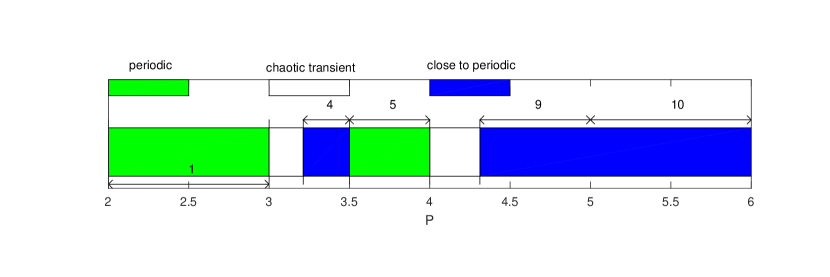
It is now helpful to rewrite the conditions in the more convenient form shown in TableΒ 1. We used the computer algebra package Mathematica to simplify each of the 2.37=4374superscript2.3743742.3^{7}=4374 combinations of subcases of the nine conditions shown in TableΒ 1 and thereby determined all possible equilibrium solutions analytically444The code and output has been deposited as ancillary material on arXiv.. The calculation took about 25 minutes on a single core of a standard desktop computer and the solutions found were then checked by hand. In total we find that there are ten distinct solutions that are valid in the ranges shown in FigureΒ 1, along with specific solutions when P=2𝑃2P=2, 333, 7/2727/2 and 555, which we label separately.

Refer to caption
Figure 1: The ranges of validity of the ten equilibrium solutions.

This illustrates the fact that there are three ranges of values of the pot size, P𝑃P, for which three equilibrium solutions coexist.

The equilibrium solutions are:

Solution 1a:​a1=b1=a2=b2=0,0≀b3≀23,c1=d2=0,formulae-sequenceSolution 1a:subscriptπ‘Ž1subscript𝑏1subscriptπ‘Ž2subscript𝑏200subscript𝑏323subscript𝑐1subscript𝑑20\mbox{\bf Solution 1a:}~{}~{}a_{1}=b_{1}=a_{2}=b_{2}=0,~{}~{}0\leq b_{3}\leq\frac{2}{3},~{}~{}c_{1}=d_{2}=0,
c3+d1≀b3,c2+d3≀b3,𝐏=𝟐.formulae-sequencesubscript𝑐3subscript𝑑1subscript𝑏3formulae-sequencesubscript𝑐2subscript𝑑3subscript𝑏3𝐏2c_{3}+d_{1}\leq b_{3},~{}~{}c_{2}+d_{3}\leq b_{3},~{}~{}{\bf P=2}.~{}~{} (5)
Solution 1:​a1=b1=a2=b2=0,b3=2P+1,c1=0,d2=2​Pβˆ’4P+1,formulae-sequenceSolution 1:subscriptπ‘Ž1subscript𝑏1subscriptπ‘Ž2subscript𝑏20formulae-sequencesubscript𝑏32𝑃1formulae-sequencesubscript𝑐10subscript𝑑22𝑃4𝑃1\mbox{\bf Solution 1:}~{}~{}a_{1}=b_{1}=a_{2}=b_{2}=0,~{}~{}b_{3}=\frac{2}{P+1},~{}~{}c_{1}=0,~{}~{}d_{2}=\frac{2P-4}{P+1},
2​Pβˆ’4P+1≀c3+d1≀2P+1,2​Pβˆ’4P+1≀c2+d3≀2P+1,πŸβ‰€πβ‰€πŸ‘.formulae-sequence2𝑃4𝑃1subscript𝑐3subscript𝑑12𝑃12𝑃4𝑃1subscript𝑐2subscript𝑑32𝑃12𝐏3\frac{2P-4}{P+1}\leq c_{3}+d_{1}\leq\frac{2}{P+1},~{}~{}\frac{2P-4}{P+1}\leq c_{2}+d_{3}\leq\frac{2}{P+1},~{}~{}{\bf 2\leq P\leq 3}.~{}~{} (6)
Solution 2a:​a1=b1=0,b2=12​a2,a2≀12,b3=12,formulae-sequenceSolution 2a:subscriptπ‘Ž1subscript𝑏10formulae-sequencesubscript𝑏212subscriptπ‘Ž2formulae-sequencesubscriptπ‘Ž212subscript𝑏312\mbox{\bf Solution 2a:}~{}~{}a_{1}=b_{1}=0,~{}~{}b_{2}=\frac{1}{2}a_{2},~{}~{}a_{2}\leq\frac{1}{2},~{}~{}b_{3}=\frac{1}{2},
c1=0,d2=12​(1+a2),c3=0,d1=12,12≀c2+d3≀12+b2,𝐏=πŸ‘.formulae-sequenceformulae-sequencesubscript𝑐10formulae-sequencesubscript𝑑2121subscriptπ‘Ž2formulae-sequencesubscript𝑐30formulae-sequencesubscript𝑑11212subscript𝑐2subscript𝑑312subscript𝑏2𝐏3c_{1}=0,~{}~{}d_{2}=\frac{1}{2}(1+a_{2}),~{}~{}c_{3}=0,~{}~{}d_{1}=\frac{1}{2},~{}~{}\frac{1}{2}\leq c_{2}+d_{3}\leq\frac{1}{2}+b_{2},~{}~{}{\bf P=3}.~{}~{} (7)
Solution 2:​a1=b1=0,a2=12,b2=1P+1,b3=2P+1,formulae-sequenceSolution 2:subscriptπ‘Ž1subscript𝑏10formulae-sequencesubscriptπ‘Ž212formulae-sequencesubscript𝑏21𝑃1subscript𝑏32𝑃1\mbox{\bf Solution 2:}~{}~{}a_{1}=b_{1}=0,~{}~{}a_{2}=\frac{1}{2},~{}~{}b_{2}=\frac{1}{P+1},~{}~{}b_{3}=\frac{2}{P+1},
c1=2​Pβˆ’6,d2=3+6​Pβˆ’2​P2P+1,c3=0,d1=2​Pβˆ’4P+1,formulae-sequencesubscript𝑐12𝑃6formulae-sequencesubscript𝑑236𝑃2superscript𝑃2𝑃1formulae-sequencesubscript𝑐30subscript𝑑12𝑃4𝑃1c_{1}=2P-6,~{}~{}d_{2}=\frac{3+6P-2P^{2}}{P+1},~{}~{}c_{3}=0,~{}~{}d_{1}=\frac{2P-4}{P+1}, (8)
2​Pβˆ’4P+1≀c2+d3≀3P+1,πŸ‘β‰€πβ‰€ππŸ’β‰‘πŸπŸβ€‹(πŸ‘+πŸπŸ“)β‰ˆ3.43.formulae-sequence2𝑃4𝑃1subscript𝑐2subscript𝑑33𝑃13𝐏subscript𝐏4123153.43~{}~{}\frac{2P-4}{P+1}\leq c_{2}+d_{3}\leq\frac{3}{P+1},~{}~{}{\bf 3\leq P\leq P_{4}\equiv\frac{1}{2}\left(3+\sqrt{15}\right)\approx 3.43}.
Solution 3:​a1=b1=0,a2=12​(4βˆ’P2+P4βˆ’4​P3+4​P2+12​P+12),b2=2​a2P+1,formulae-sequenceSolution 3:subscriptπ‘Ž1subscript𝑏10formulae-sequencesubscriptπ‘Ž2124superscript𝑃2superscript𝑃44superscript𝑃34superscript𝑃212𝑃12subscript𝑏22subscriptπ‘Ž2𝑃1\mbox{\bf Solution 3:}~{}~{}a_{1}=b_{1}=0,~{}~{}a_{2}=\frac{1}{2}\left(4-P^{2}+\sqrt{P^{4}-4P^{3}+4P^{2}+12P+12}\right),~{}~{}b_{2}=\frac{2a_{2}}{P+1},
b3=2βˆ’b2P+a2,c1=2​Pβˆ’4+2​a2P+1,d2=0,c3=0,d1=2​Pβˆ’4P+1,formulae-sequencesubscript𝑏32subscript𝑏2𝑃subscriptπ‘Ž2formulae-sequencesubscript𝑐12𝑃42subscriptπ‘Ž2𝑃1formulae-sequencesubscript𝑑20formulae-sequencesubscript𝑐30subscript𝑑12𝑃4𝑃1b_{3}=\frac{2-b_{2}}{P+a_{2}},~{}~{}c_{1}=\frac{2P-4+2a_{2}}{P+1},~{}~{}d_{2}=0,~{}~{}c_{3}=0,~{}~{}d_{1}=\frac{2P-4}{P+1}, (9)
2​Pβˆ’4P+1≀c2+d3≀b2+b3,ππŸ‘β‰‘πŸπŸ’β€‹(πŸ‘+πŸ—πŸ•)β‰ˆ3.21β‰€πβ‰€ππŸ’β‰‘πŸπŸβ€‹(πŸ‘+πŸπŸ“)β‰ˆ3.43.formulae-sequence2𝑃4𝑃1subscript𝑐2subscript𝑑3subscript𝑏2subscript𝑏3subscript𝐏3143973.21𝐏subscript𝐏4123153.43\frac{2P-4}{P+1}\leq c_{2}+d_{3}\leq b_{2}+b_{3},~{}~{}{\bf P_{3}\equiv\frac{1}{4}\left(3+\sqrt{97}\right)\approx 3.21\leq P\leq P_{4}\equiv\frac{1}{2}\left(3+\sqrt{15}\right)\approx 3.43}.
Solution 4:​a1=b1=0,a2=12​(5βˆ’P),b2=5βˆ’PP+1,b3=4​(Pβˆ’2)3​(P+1),formulae-sequenceSolution 4:subscriptπ‘Ž1subscript𝑏10formulae-sequencesubscriptπ‘Ž2125𝑃formulae-sequencesubscript𝑏25𝑃𝑃1subscript𝑏34𝑃23𝑃1\mbox{\bf Solution 4:}~{}~{}a_{1}=b_{1}=0,~{}~{}a_{2}=\frac{1}{2}(5-P),~{}~{}b_{2}=\frac{5-P}{P+1},~{}~{}b_{3}=\frac{4(P-2)}{3(P+1)},
c1=1,d2=0,c3=0,d1=2​Pβˆ’4P+1,formulae-sequencesubscript𝑐11formulae-sequencesubscript𝑑20formulae-sequencesubscript𝑐30subscript𝑑12𝑃4𝑃1c_{1}=1,~{}~{}d_{2}=0,~{}~{}c_{3}=0,~{}~{}d_{1}=\frac{2P-4}{P+1}, (10)
2​Pβˆ’4P+1≀c2+d3≀P+73​(P+1),ππŸ‘β‰‘πŸπŸ’β€‹(πŸ‘+πŸ—πŸ•)β‰ˆ3.21β‰€πβ‰€πŸ•πŸ.formulae-sequence2𝑃4𝑃1subscript𝑐2subscript𝑑3𝑃73𝑃1subscript𝐏3143973.21𝐏72\frac{2P-4}{P+1}\leq c_{2}+d_{3}\leq\frac{P+7}{3(P+1)},~{}~{}{\bf P_{3}\equiv\frac{1}{4}\left(3+\sqrt{97}\right)\approx 3.21\leq P\leq\frac{7}{2}}.
Solution 5a:​a1=b1=0,b2=49​a2,a2β‰₯34,b3=49,formulae-sequenceSolution 5a:subscriptπ‘Ž1subscript𝑏10formulae-sequencesubscript𝑏249subscriptπ‘Ž2formulae-sequencesubscriptπ‘Ž234subscript𝑏349\mbox{\bf Solution 5a:}~{}~{}a_{1}=b_{1}=0,~{}~{}b_{2}=\frac{4}{9}a_{2},~{}~{}a_{2}\geq\frac{3}{4},~{}~{}b_{3}=\frac{4}{9},
c1=1,d2=49​a2βˆ’13,c3=0,d1=23,formulae-sequencesubscript𝑐11formulae-sequencesubscript𝑑249subscriptπ‘Ž213formulae-sequencesubscript𝑐30subscript𝑑123c_{1}=1,~{}~{}d_{2}=\frac{4}{9}a_{2}-\frac{1}{3},~{}~{}c_{3}=0,~{}~{}d_{1}=\frac{2}{3}, (11)
23≀c2+d3≀49​(1+a2),𝐏=πŸ•πŸ.formulae-sequence23subscript𝑐2subscript𝑑3491subscriptπ‘Ž2𝐏72\frac{2}{3}\leq c_{2}+d_{3}\leq\frac{4}{9}(1+a_{2}),~{}~{}{\bf P=\frac{7}{2}}.
Solution 5:​a1=b1=0,a2=1,b2=2P+1,b3=2P+1,formulae-sequenceSolution 5:subscriptπ‘Ž1subscript𝑏10formulae-sequencesubscriptπ‘Ž21formulae-sequencesubscript𝑏22𝑃1subscript𝑏32𝑃1\mbox{\bf Solution 5:}~{}~{}a_{1}=b_{1}=0,~{}~{}a_{2}=1,~{}~{}b_{2}=\frac{2}{P+1},~{}~{}b_{3}=\frac{2}{P+1},
c1=1,d2=Pβˆ’3P+1,c3=0,d1=2​Pβˆ’4P+1,formulae-sequencesubscript𝑐11formulae-sequencesubscript𝑑2𝑃3𝑃1formulae-sequencesubscript𝑐30subscript𝑑12𝑃4𝑃1c_{1}=1,~{}~{}d_{2}=\frac{P-3}{P+1},~{}~{}c_{3}=0,~{}~{}d_{1}=\frac{2P-4}{P+1}, (12)
2​Pβˆ’4P+1≀c2+d3≀4P+1,πŸ•πŸβ‰€πβ‰€πŸ’.formulae-sequence2𝑃4𝑃1subscript𝑐2subscript𝑑34𝑃172𝐏4\frac{2P-4}{P+1}\leq c_{2}+d_{3}\leq\frac{4}{P+1},~{}~{}{\bf\frac{7}{2}\leq P\leq 4}.
Solution 6:​a1=(4βˆ’P)​(P+1),b1=2​(4βˆ’P),a2=1,b2=2P+1,formulae-sequenceSolution 6:subscriptπ‘Ž14𝑃𝑃1formulae-sequencesubscript𝑏124𝑃formulae-sequencesubscriptπ‘Ž21subscript𝑏22𝑃1\mbox{\bf Solution 6:}~{}~{}a_{1}=(4-P)(P+1),~{}~{}b_{1}=2(4-P),~{}~{}a_{2}=1,~{}~{}b_{2}=\frac{2}{P+1},
b3=2​(Pβˆ’3)P+1,c1=1,d2=5+7​Pβˆ’2​P2P+1,c3=0,d1=4+8​Pβˆ’2​P2P+1,formulae-sequencesubscript𝑏32𝑃3𝑃1formulae-sequencesubscript𝑐11formulae-sequencesubscript𝑑257𝑃2superscript𝑃2𝑃1formulae-sequencesubscript𝑐30subscript𝑑148𝑃2superscript𝑃2𝑃1b_{3}=\frac{2(P-3)}{P+1},~{}~{}c_{1}=1,~{}~{}d_{2}=\frac{5+7P-2P^{2}}{P+1},~{}~{}c_{3}=0,~{}~{}d_{1}=\frac{4+8P-2P^{2}}{P+1}, (13)
c2=0,d3=2​Pβˆ’4P+1,ππŸ”β‰‘πŸπŸβ€‹(πŸ‘+πŸπŸ‘)β‰ˆ3.90β‰€πβ‰€πŸ’.formulae-sequencesubscript𝑐20formulae-sequencesubscript𝑑32𝑃4𝑃1subscript𝐏6123233.90𝐏4c_{2}=0,~{}~{}d_{3}=\frac{2P-4}{P+1},~{}~{}{\bf P_{6}\equiv\frac{1}{2}\left(3+\sqrt{23}\right)\approx 3.90\leq P\leq 4}.
Solution 7:​a1=12,b1=1P+1,a2=1,b2=2P+1,b3=2​P+1(P+1)2,formulae-sequenceSolution 7:subscriptπ‘Ž112formulae-sequencesubscript𝑏11𝑃1formulae-sequencesubscriptπ‘Ž21formulae-sequencesubscript𝑏22𝑃1subscript𝑏32𝑃1superscript𝑃12\mbox{\bf Solution 7:}~{}~{}a_{1}=\frac{1}{2},~{}~{}b_{1}=\frac{1}{P+1},~{}~{}a_{2}=1,~{}~{}b_{2}=\frac{2}{P+1},~{}~{}b_{3}=\frac{2P+1}{(P+1)^{2}},
c1=1,d2=Pβˆ’2P+1,c3=2​P2βˆ’6​Pβˆ’7P+1,d1=4+8​Pβˆ’2​P2P+1,c2=0,formulae-sequencesubscript𝑐11formulae-sequencesubscript𝑑2𝑃2𝑃1formulae-sequencesubscript𝑐32superscript𝑃26𝑃7𝑃1formulae-sequencesubscript𝑑148𝑃2superscript𝑃2𝑃1subscript𝑐20c_{1}=1,~{}~{}d_{2}=\frac{P-2}{P+1},~{}~{}c_{3}=\frac{2P^{2}-6P-7}{P+1},~{}~{}d_{1}=\frac{4+8P-2P^{2}}{P+1},~{}~{}c_{2}=0, (14)
d3=2​Pβˆ’4P+1,ππŸ”β‰‘πŸπŸβ€‹(πŸ‘+πŸπŸ‘)β‰ˆ3.90β‰€πβ‰€ππŸ—β‰‘πŸπŸ’β€‹(πŸ•+πŸπŸπŸ‘)β‰ˆ4.41.formulae-sequencesubscript𝑑32𝑃4𝑃1subscript𝐏6123233.90𝐏subscript𝐏91471134.41d_{3}=\frac{2P-4}{P+1},~{}~{}{\bf P_{6}\equiv\frac{1}{2}\left(3+\sqrt{23}\right)\approx 3.90\leq P\leq P_{9}\equiv\frac{1}{4}\left(7+\sqrt{113}\right)\approx 4.41}.
Solution 8:​a1=12​(9βˆ’2​P)​(P+1),b1=9βˆ’2​P,a2=1,b2=2P+1,b3=2​Pβˆ’7P+1,formulae-sequenceSolution 8:subscriptπ‘Ž11292𝑃𝑃1formulae-sequencesubscript𝑏192𝑃formulae-sequencesubscriptπ‘Ž21formulae-sequencesubscript𝑏22𝑃1subscript𝑏32𝑃7𝑃1\mbox{\bf Solution 8:}~{}~{}a_{1}=\frac{1}{2}(9-2P)(P+1),~{}~{}b_{1}=9-2P,~{}~{}a_{2}=1,~{}~{}b_{2}=\frac{2}{P+1},~{}~{}b_{3}=\frac{2P-7}{P+1},
c1=1,d2=6+8​Pβˆ’2​P2P+1,c3=1,d1=4+8​Pβˆ’2​P2P+1,c2=0,formulae-sequencesubscript𝑐11formulae-sequencesubscript𝑑268𝑃2superscript𝑃2𝑃1formulae-sequencesubscript𝑐31formulae-sequencesubscript𝑑148𝑃2superscript𝑃2𝑃1subscript𝑐20c_{1}=1,~{}~{}d_{2}=\frac{6+8P-2P^{2}}{P+1},~{}~{}c_{3}=1,~{}~{}d_{1}=\frac{4+8P-2P^{2}}{P+1},~{}~{}c_{2}=0, (15)
d3=2​Pβˆ’4P+1,ππŸ–β‰‘πŸπŸ’β€‹(πŸ•+πŸπŸŽπŸ“)β‰ˆ4.31β‰€πβ‰€ππŸ—β‰‘πŸπŸ’β€‹(πŸ•+πŸπŸπŸ‘)β‰ˆ4.41.formulae-sequencesubscript𝑑32𝑃4𝑃1subscript𝐏81471054.31𝐏subscript𝐏91471134.41d_{3}=\frac{2P-4}{P+1},~{}~{}{\bf P_{8}\equiv\frac{1}{4}\left(7+\sqrt{105}\right)\approx 4.31\leq P\leq P_{9}\equiv\frac{1}{4}\left(7+\sqrt{113}\right)\approx 4.41}.
Solution 9:​a1=1,b1=2P+1,a2=1,b2=2P+1,b3=2​P(P+1)2,formulae-sequenceSolution 9:subscriptπ‘Ž11formulae-sequencesubscript𝑏12𝑃1formulae-sequencesubscriptπ‘Ž21formulae-sequencesubscript𝑏22𝑃1subscript𝑏32𝑃superscript𝑃12\mbox{\bf Solution 9:}~{}~{}a_{1}=1,~{}~{}b_{1}=\frac{2}{P+1},~{}~{}a_{2}=1,~{}~{}b_{2}=\frac{2}{P+1},~{}~{}b_{3}=\frac{2P}{(P+1)^{2}},
c1+d2=2​PP+1,c3=1,d1=Pβˆ’3P+1,c2=0,formulae-sequencesubscript𝑐1subscript𝑑22𝑃𝑃1formulae-sequencesubscript𝑐31formulae-sequencesubscript𝑑1𝑃3𝑃1subscript𝑐20c_{1}+d_{2}=\frac{2P}{P+1},~{}~{}c_{3}=1,~{}~{}d_{1}=\frac{P-3}{P+1},~{}~{}c_{2}=0, (16)
d3=2​Pβˆ’4P+1,ππŸ–β‰‘πŸπŸ’β€‹(πŸ•+πŸπŸŽπŸ“)β‰ˆ4.31β‰€πβ‰€πŸ“.formulae-sequencesubscript𝑑32𝑃4𝑃1subscript𝐏81471054.31𝐏5d_{3}=\frac{2P-4}{P+1},~{}~{}{\bf P_{8}\equiv\frac{1}{4}\left(7+\sqrt{105}\right)\approx 4.31\leq P\leq 5}.
Solution 10a:​a1=1,13≀b1≀25,a2=1,b2=13,b3=518,formulae-sequenceformulae-sequenceSolution 10a:subscriptπ‘Ž1113subscript𝑏125formulae-sequencesubscriptπ‘Ž21formulae-sequencesubscript𝑏213subscript𝑏3518\mbox{\bf Solution 10a:}~{}~{}a_{1}=1,~{}~{}\frac{1}{3}\leq b_{1}\leq\frac{2}{5},~{}~{}a_{2}=1,~{}~{}b_{2}=\frac{1}{3},~{}~{}b_{3}=\frac{5}{18},
c1+d2=53​whenΒ b1=13,c1=23,d2=1​whenΒ b1>13,formulae-sequencesubscript𝑐1subscript𝑑253whenΒ b1=13,formulae-sequencesubscript𝑐123subscript𝑑21whenΒ b1>13,c_{1}+d_{2}=\frac{5}{3}~{}\mbox{when $b_{1}=\dfrac{1}{3}$,}~{}~{}~{}~{}c_{1}=\frac{2}{3},~{}d_{2}=1~{}\mbox{when $b_{1}>\dfrac{1}{3}$,} (17)
c3=1,d1=13,c2=0,d3=1,𝐏=πŸ“.formulae-sequencesubscript𝑐31formulae-sequencesubscript𝑑113formulae-sequencesubscript𝑐20formulae-sequencesubscript𝑑31𝐏5c_{3}=1,~{}~{}d_{1}=\frac{1}{3},~{}~{}c_{2}=0,~{}~{}d_{3}=1,~{}~{}{\bf P=5}.
Solution 10:​a1=1,b1=2P,a2=1,b2=2P+1,b3=2​P(P+1)2,formulae-sequenceSolution 10:subscriptπ‘Ž11formulae-sequencesubscript𝑏12𝑃formulae-sequencesubscriptπ‘Ž21formulae-sequencesubscript𝑏22𝑃1subscript𝑏32𝑃superscript𝑃12\mbox{\bf Solution 10:}~{}~{}a_{1}=1,~{}~{}b_{1}=\frac{2}{P},~{}~{}a_{2}=1,~{}~{}b_{2}=\frac{2}{P+1},~{}~{}b_{3}=\frac{2P}{(P+1)^{2}},
c1=Pβˆ’1P+1,d2=1,c3=1,d1=Pβˆ’3P+1,c2=Pβˆ’5P+1,formulae-sequencesubscript𝑐1𝑃1𝑃1formulae-sequencesubscript𝑑21formulae-sequencesubscript𝑐31formulae-sequencesubscript𝑑1𝑃3𝑃1subscript𝑐2𝑃5𝑃1c_{1}=\frac{P-1}{P+1},~{}~{}d_{2}=1,~{}~{}c_{3}=1,~{}~{}d_{1}=\frac{P-3}{P+1},~{}~{}c_{2}=\frac{P-5}{P+1}, (18)
d3=1,𝐏β‰₯πŸ“.formulae-sequencesubscript𝑑31𝐏5d_{3}=1,~{}~{}{\bf P\geq 5}.

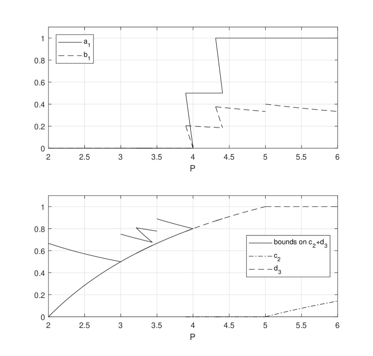
FigureΒ 2 shows the equilibrium frequencies at which Player 1 bets and Players 2 and 3 call. For small enough P (P<P6β‰ˆ3.9𝑃subscript𝑃63.9P<P_{6}\approx 3.9), Player 1 neither bets with A nor bluffs with Q at equilibrium. For these values of P𝑃P, the solid lines in the lower graph show the bounds between which c2+d3subscript𝑐2subscript𝑑3c_{2}+d_{3} must lie at equilibrium. For values above the upper bound, Player 1 can exploit her opponents by always betting with A; for values below the lower bound, by always bluffing with Q. For larger values of P𝑃P, Player 1 has nonzero betting and bluffing frequencies at equilibrium, including two ranges of P𝑃P with multiple solutions. Only Player 3 catches Player 1’s bluffs for P<5𝑃5P<5, whilst for P>5𝑃5P>5, Player 1 always calls with K and Player 2 also catches bluffs with K at a nonzero frequency (d3=1subscript𝑑31d_{3}=1, c2>0subscript𝑐20c_{2}>0).

Refer to caption
Figure 2: Player 1’s equilibrium betting frequencies and the consequent calling frequencies.

FigureΒ 3 shows the equilibrium frequencies at which Player 2 bets and Players 3 and 1 call. For P<3𝑃3P<3, Player 2 does not bet at equilibrium, and there are upper and lower bounds on c3+d1subscript𝑐3subscript𝑑1c_{3}+d_{1}. For P>3𝑃3P>3, Player 2 bets at equilibrium, with one range of multiple solutions. Players 3 and 1 have calling frequencies that have a rather unintuitive structure at equilibrium. For small enough P𝑃P, Player 1 is the bluffcatcher, but as P𝑃P increases, Player 3 develops a nonzero equilibrium calling frequency. For large enough P𝑃P, Player 3 always calls with K and Player 1 has a nonzero calling frequency. This is in contrast to the frequencies shown in FigureΒ 2, where the player who acts immediately after the original bettor (Player 2) does not call with K for small enough values of P𝑃P, but the next player to act (Player 3) does.
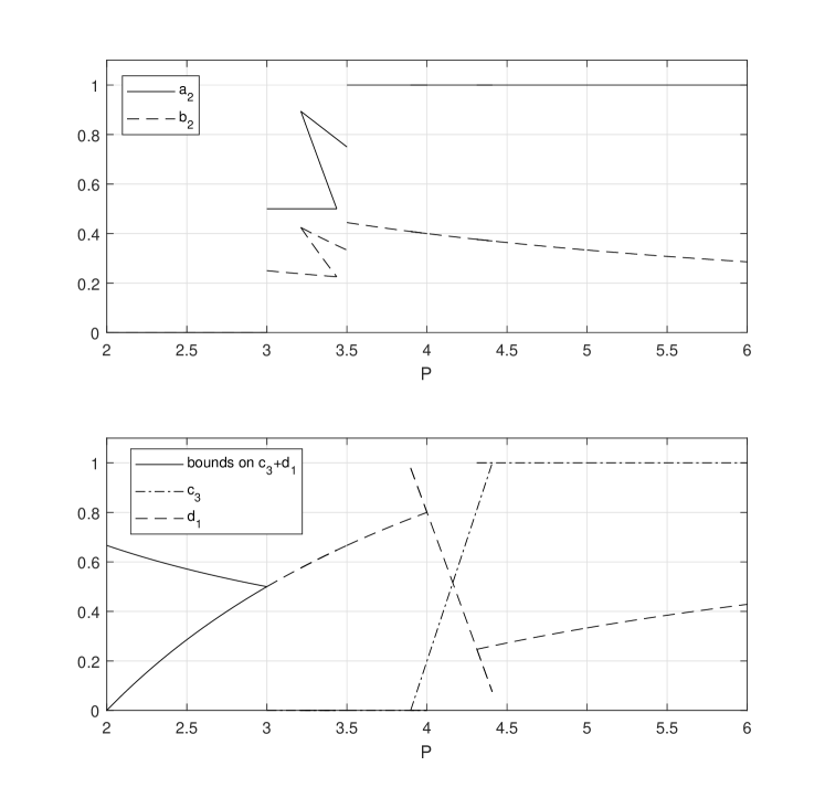
Refer to caption
Figure 3: Player 2’s equilibrium betting frequencies and the consequent calling frequencies.

FigureΒ 4 shows the equilibrium frequencies at which Player 3 bluffs and Players 1 and 2 call. Since Player 3 always bets with A, she has a nonzero bluffing frequency for all P𝑃P, which generally decreases as P𝑃P increases, with some irregular behaviour in the regions where three equilibrium solutions exist. The most notable feature of the calling frequencies of Players 1 and 2 is that there is a set of values of P𝑃P for which Player 1 always calls with K (c1=1subscript𝑐11c_{1}=1), followed by a region where there is a range of possible values of c1subscript𝑐1c_{1} and d1subscript𝑑1d_{1}, bounded by the solid lines, followed for large enough P𝑃P by a set of values for which Player 2 always calls with K (d2=1subscript𝑑21d_{2}=1). It is hard to interpret these equilibrium solutions, in particular the peculiar way in which the calling frequencies vary with P𝑃P, either mathematically or in terms of poker concepts.
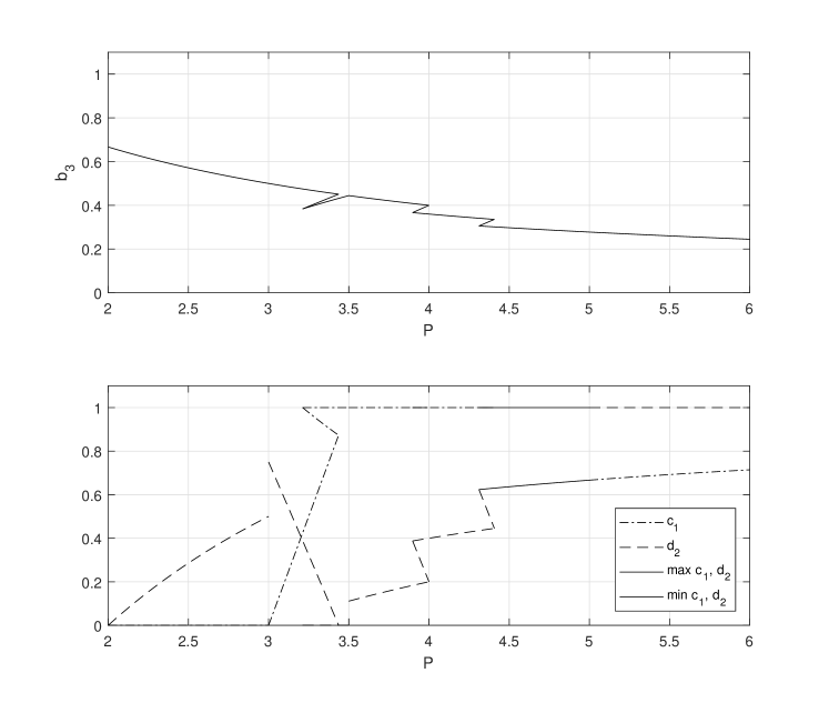
Refer to caption
Figure 4: Player 3’s equilibrium bluffing frequency and the consequent calling frequencies.

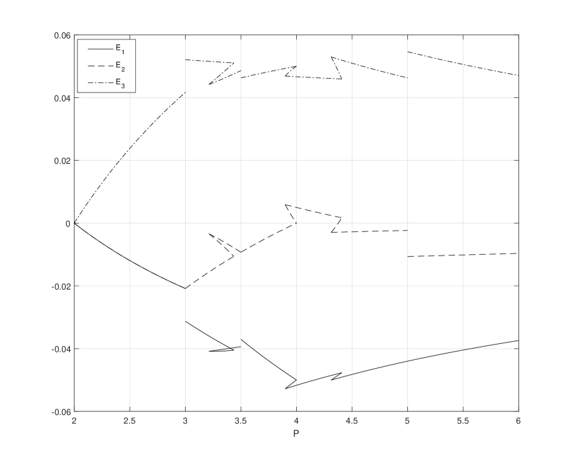
The expected profits of each player can be calculated using (1) to (3), and are shown in FigureΒ 5.

Refer to caption
Figure 5: The expected profits at equilibrium.

Although the existence of multiple equilibrium solutions makes the structure of these curves quite irregular, Player 3 always has the largest expected profit, because she acts last, whilst for P>3𝑃3P>3, when Player 2 develops a nonzero equilibrium betting frequency, Player 2 has a larger expected profit than Player 1, because she acts after Player 1.

It is also of interest to consider the expected profits for Solutions 2a, 5a and 10a, which are

Solution 2a (P=3):​24​E1=βˆ’12βˆ’12​a2,24​E2=βˆ’12,24​E3=1+12​a2,a2≀12.formulae-sequenceSolution 2a (P=3):24subscript𝐸11212subscriptπ‘Ž2formulae-sequence24subscript𝐸212formulae-sequence24subscript𝐸3112subscriptπ‘Ž2subscriptπ‘Ž212\mbox{\bf Solution 2a ($P=3$):}~{}24E_{1}=-\frac{1}{2}-\frac{1}{2}a_{2},~{}~{}24E_{2}=-\frac{1}{2},~{}~{}24E_{3}=1+\frac{1}{2}a_{2},~{}~{}a_{2}\leq\frac{1}{2}. (19)
Solution 5a (P=72):​24​E1=βˆ’109+29​a2,24​E2=βˆ’29,24​E3=43βˆ’29​a2​a2β‰₯34.formulae-sequenceSolution 5a (P=72):24subscript𝐸110929subscriptπ‘Ž2formulae-sequence24subscript𝐸22924subscript𝐸34329subscriptπ‘Ž2subscriptπ‘Ž234\mbox{\bf Solution 5a ($P=\dfrac{7}{2}$):}~{}24E_{1}=-\frac{10}{9}+\frac{2}{9}a_{2},~{}~{}24E_{2}=-\frac{2}{9},~{}~{}24E_{3}=\frac{4}{3}-\frac{2}{9}a_{2}~{}~{}a_{2}\geq\frac{3}{4}. (20)
Solution 10a (P=5):​24​E1=βˆ’1918,24​E2=1718βˆ’3​b1,24​E3=19+3​b1,13≀b1≀25.formulae-sequenceSolution 10a (P=5):24subscript𝐸11918formulae-sequence24subscript𝐸217183subscript𝑏1formulae-sequence24subscript𝐸3193subscript𝑏113subscript𝑏125\mbox{\bf Solution 10a ($P=5$):}~{}24E_{1}=-\frac{19}{18},~{}~{}24E_{2}=\frac{17}{18}-3b_{1},~{}~{}24E_{3}=\frac{1}{9}+3b_{1},~{}~{}\frac{1}{3}\leq b_{1}\leq\frac{2}{5}. (21)

In Solutions 2a and 5a, Player 2 can transfer profit between Players 1 and 3 at no cost to herself, although it should be noted that for Solution 5a, with P=72𝑃72P=\frac{7}{2}, the equilibrium solution is not unique. In Solution 10a, Player 1 can transfer profit between Players 2 and 3 at no cost to herself. In each case, this can be seen as points of discontinuity in the expected profits plotted in FigureΒ 5. This may have implications for repeated play of the game at these pot sizes, as discussed for the one-third street game in [1] and [5].

In two player, zero sum games, such as two player Kuhn poker, all equilibrium solutions have the same expected profit. This is not the case for the three player zero sum game that we study here. Moreover, although finding the equilibrium solutions is important, it is the dynamics of the play of the game, which may or may not lead the players towards an equilibrium solution, that determine the outcome of repeated play.

4 An ordinary differential equation model of repeated play

In [1] we studied an ordinary differential equation model of a simplified version of one-third street Kuhn poker. The dynamics are always oscillatory, with only one player bluffcatching, and the identity of that player determined by the initial betting frequencies. We also showed that a more realistic model, which is based on repeated play of the game, has similar dynamics, provided that the players neither adjust their frequencies too rapidly nor have too long a memory. In this section we will study an ordinary differential equation model of the dynamics of repeated play of the simplified full street game. We find that a wider range of dynamics is available than was possible for the system studied in [1].

4.1 The ordinary differential equation model

We assume that Player i𝑖i controls the four frequencies ai​(t)subscriptπ‘Žπ‘–π‘‘a_{i}(t), bi​(t)subscript𝑏𝑖𝑑b_{i}(t), ci​(t)subscript𝑐𝑖𝑑c_{i}(t) and di​(t)subscript𝑑𝑖𝑑d_{i}(t) (three frequencies for Player 3, since betting with A is the dominant strategy, which means that a3=1subscriptπ‘Ž31a_{3}=1) in order to try to maximise their expected value. For example, we model the behaviour of Player 1’s betting frequency, a1​(t)subscriptπ‘Ž1𝑑a_{1}(t), using

d​a1d​t=24​k1​a1​(1βˆ’a1)β€‹βˆ‚E1βˆ‚a1≑k1​a1​(1βˆ’a1)​(βˆ’2​b2+2​c2βˆ’2​b3+2​d3βˆ’b2​c3),𝑑subscriptπ‘Ž1𝑑𝑑24subscriptπ‘˜1subscriptπ‘Ž11subscriptπ‘Ž1subscript𝐸1subscriptπ‘Ž1subscriptπ‘˜1subscriptπ‘Ž11subscriptπ‘Ž12subscript𝑏22subscript𝑐22subscript𝑏32subscript𝑑3subscript𝑏2subscript𝑐3\frac{da_{1}}{dt}=24k_{1}a_{1}\left(1-a_{1}\right)\frac{\partial E_{1}}{\partial a_{1}}\equiv k_{1}a_{1}\left(1-a_{1}\right)\left(-2b_{2}+2c_{2}-2b_{3}+2d_{3}-b_{2}c_{3}\right), (22)

where k1subscriptπ‘˜1k_{1} is a positive constant555The factor of 24 is purely for computational convenience. It has no effect on the qualitative nature of the dynamics of the system.. Each frequency fisubscript𝑓𝑖f_{i} satisfies

d​fid​t=24​kj​fi​(1βˆ’fi)β€‹βˆ‚Eiβˆ‚fi,𝑑subscript𝑓𝑖𝑑𝑑24subscriptπ‘˜π‘—subscript𝑓𝑖1subscript𝑓𝑖subscript𝐸𝑖subscript𝑓𝑖\frac{df_{i}}{dt}=24k_{j}f_{i}\left(1-f_{i}\right)\frac{\partial E_{i}}{\partial f_{i}}, (23)

where kjsubscriptπ‘˜π‘—k_{j} are positive constants. The term fi​(1βˆ’fi)subscript𝑓𝑖1subscript𝑓𝑖f_{i}(1-f_{i}) constrains fisubscript𝑓𝑖f_{i} to lie in [0,1]01[0,1], and also means that, since d​fi/d​t=0𝑑subscript𝑓𝑖𝑑𝑑0df_{i}/dt=0 when fi=0subscript𝑓𝑖0f_{i}=0 or fi=1subscript𝑓𝑖1f_{i}=1, all of the equilibrium solutions of the game discussed in SectionΒ 3 are also equilibrium solutions of the system of eleven nonlinear ordinary differential equations defined by (23). There also exist equilibrium solutions of the differential equations that are not equilibrium solutions of the game because they do not satisfy one of the constraints on the sign of βˆ‚Ei/βˆ‚fisubscript𝐸𝑖subscript𝑓𝑖\partial E_{i}/\partial f_{i} (see TableΒ 1). However, for precisely this reason, these equilibrium solutions are unstable with respect to the dynamics imposed by the differential equations.

From this point onwards, we will fix kj=1subscriptπ‘˜π‘—1k_{j}=1 for j=1𝑗1j=1, 222 …111111 to reduce the complexity of the system. The dynamics of this system can be either periodic, close to periodic or have a long, chaotic transient before being attracted to the boundary of the phase space (fi=0subscript𝑓𝑖0f_{i}=0 or fi=1subscript𝑓𝑖1f_{i}=1 for i=1𝑖1i=1, 222, 333), depending on the size, P𝑃P, of the pot. The solution does not asymptote to a steady, stable equilibrium state for any nonequilibrium initial conditions or pot size P𝑃P for which we solved the equations. We find, through numerical computation of the eigenvalues of each of the equilibrium points given by (6) to (18), that Solutions 2, 3, 6, 7 and 8 are unstable. None of Solutions 1, 4, 5, 9 and 10 are asymptotically stable, because each has a centre manifold, but numerical solutions suggest that they are all Lyapunov stable. In other words, solutions that start close to these equilibrium points remain nearby, but do not asymptote to equilibrium as tβ†’βˆžβ†’π‘‘t\to\infty. Instead, the solutions are attracted to the centre manifold, where the dynamics are oscillatory. The oscillatory part of the centre manifold has either two dimensions (Solution 1), four dimensions (Solutions 4 and 5), or six dimensions (Solutions 9 and 10). This will become apparent in the nature of the solutions that we discuss below. The increase in the dimensionality of the oscillatory part of the centre manifold reflects the fact that as the pot size, P𝑃P, increases, Player 2, and then for larger P𝑃P, Player 1, has a nonzero bluffing frequency. For 3<P<P3β‰ˆ3.213𝑃subscript𝑃33.213<P<P_{3}\approx 3.21 and 4<P<P8β‰ˆ4.314𝑃subscript𝑃84.314<P<P_{8}\approx 4.31 all equilibrium points are unstable, and we observe long chaotic transients before the solution asymptotes to the boundary of the phase space, with each betting frequency close to zero or one. Finally, we note that, unlike the ordinary differential equation model studied in [1], where the initial betting frequencies determined which of two qualitatively different types of periodic solution emerged as the long time solution, only one type of behaviour is observed for each P𝑃P that we studied, but with amplitude dependent on the initial betting frequencies.

4.2 Numerical solution

In order to solve (23) accurately when the betting frequencies are close to zero and one, we solved for the dependent variables Fi≑log⁑{fi/(1βˆ’fi)}subscript𝐹𝑖subscript𝑓𝑖1subscript𝑓𝑖F_{i}\equiv\log\left\{f_{i}/\left(1-f_{i}\right)\right\} instead of fisubscript𝑓𝑖f_{i}, in terms of which (23) take the simpler form

d​Fid​t=24​kjβ€‹βˆ‚Eiβˆ‚fi.𝑑subscript𝐹𝑖𝑑𝑑24subscriptπ‘˜π‘—subscript𝐸𝑖subscript𝑓𝑖\frac{dF_{i}}{dt}=24k_{j}\frac{\partial E_{i}}{\partial f_{i}}. (24)

We solved the system of equations (24) using the fifth order Runge-Kutta solver ode45 in MATLAB. FigureΒ 6 shows schematically how the qualitative nature of the dynamics of solutions of (23) varies with pot size, P𝑃P. We will give an example of a typical solution from each of these six ranges of values of P𝑃P. We refer to some of the transient behaviour of the solutions as ’chaotic’, but note that we have not attempted to study the nature of this in any detail. Our study of this model is only meant to illustrate that the dynamics can be far more complex than those of repeated two player, zero sum games.
Refer to caption
Figure 6: The Lyapunov stable equilibrium solutions, 1, 4, 5, 9 and 10 along with color codes for the behaviour of solutions. Green = periodic; White = chaotic transient; Blue = close to periodic.

4.2.1 Case 1: 2<P<32𝑃32<P<3

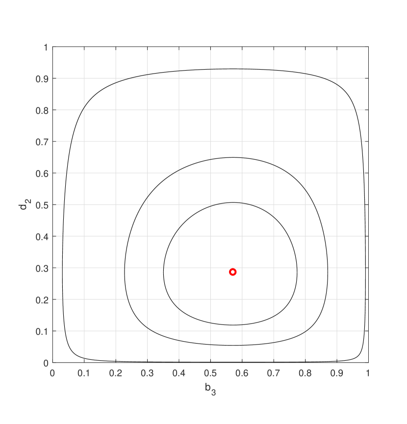
In this case a1β†’0β†’subscriptπ‘Ž10a_{1}\to 0, a2β†’0β†’subscriptπ‘Ž20a_{2}\to 0 and c1β†’0β†’subscript𝑐10c_{1}\to 0 as tβ†’βˆžβ†’π‘‘t\to\infty. The only nontrivial betting frequencies are b3subscript𝑏3b_{3} and d2subscript𝑑2d_{2}, which vary periodically with amplitude depending on the initial conditions, as shown in FigureΒ 7 for P=2.5𝑃2.5P=2.5 and three different values of the initial betting frequencies. The centre manifold of Solution 1 attracts the solution. Player 3’s bluffing frequency rises and falls, and Player 2, who does the bluff catching, adjusts her calling frequency in response. This behaviour is typical of solutions for 2<P<32𝑃32<P<3 and is the only case for which the dynamics are similar to those of the system studied in [1].
Refer to caption
Figure 7: The behaviour of Player 3’s bluffing frequency and Player 2’s calling frequency for three different sets of initial betting frequencies when P=2.5𝑃2.5P=2.5. Solution 1 is marked with a red circle.

4.3 Case 2: 3<P<P3β‰ˆ3.213𝑃subscript𝑃33.213<P<P_{3}\approx 3.21

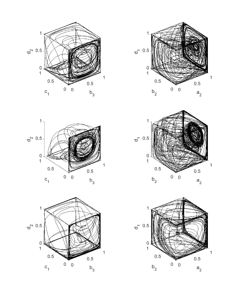
In this case, all equilibrium solutions are unstable. Although a1β†’0β†’subscriptπ‘Ž10a_{1}\to 0, b1β†’0β†’subscript𝑏10b_{1}\to 0 and c3β†’0β†’subscript𝑐30c_{3}\to 0 as tβ†’βˆžβ†’π‘‘t\to\infty, the dynamics of b3subscript𝑏3b_{3}, c1subscript𝑐1c_{1}, d2subscript𝑑2d_{2}, a2subscriptπ‘Ž2a_{2}, b2subscript𝑏2b_{2} and d1subscript𝑑1d_{1} are complicated, and strongly dependent on the initial betting frequencies, as shown in FigureΒ 8 for P=3.1𝑃3.1P=3.1 and three different values of the initial betting frequencies. Although the initial transient behaviour appears chaotic and typically lasts until t𝑑t is between 103superscript10310^{3} and 104superscript10410^{4}, the solution eventually asymptotes to the boundary of the phase space, with each betting frequency close to zero or one. This is likely to be an artefact of the way we have chosen the differential equations (specifically the fi​(1βˆ’fi)subscript𝑓𝑖1subscript𝑓𝑖f_{i}(1-f_{i}) terms), and we should simply take it as an indication that the dynamics are nontrivial for this range of pot sizes, for which this behaviour is typical. Similar comments apply in Cases 5 and 6 below.
Refer to caption
Figure 8: Chaotic transient behaviour when P=3.1𝑃3.1P=3.1 for three different initial conditions.

4.4 Case 3: P3β‰ˆ3.21<P<3.5subscript𝑃33.21𝑃3.5P_{3}\approx 3.21<P<3.5

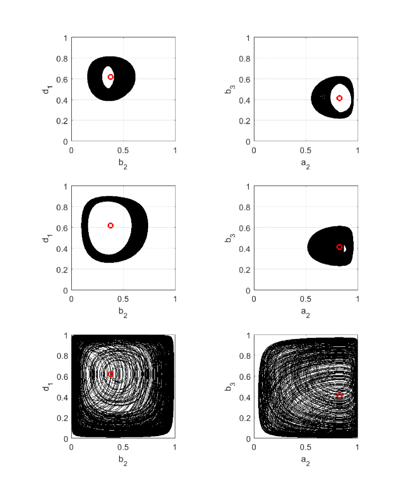
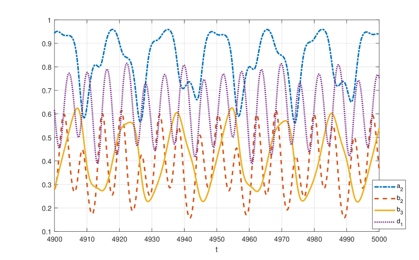
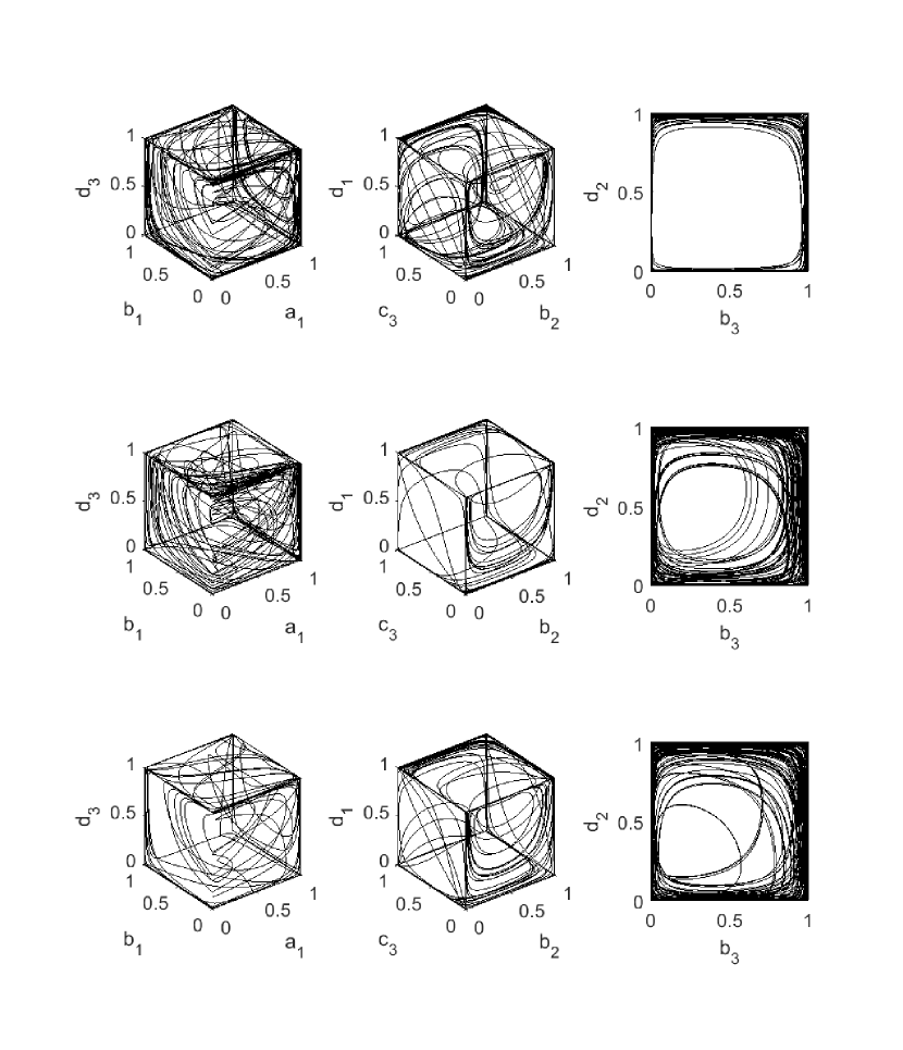
Solution 4 is Lyapunov stable, but not asymptotically stable, and solutions are attracted to its centre manifold, the oscillatory part of which is four-dimensional. The nontrivial betting frequencies are a2subscriptπ‘Ž2a_{2}, b2subscript𝑏2b_{2}, d1subscript𝑑1d_{1} and b3subscript𝑏3b_{3}, consistent with the local behaviour of the centre manifold. Some typical solutions are shown in FiguresΒ 9 andΒ 10. Note that a2subscriptπ‘Ž2a_{2}, b2subscript𝑏2b_{2} and d1subscript𝑑1d_{1} are related to adjustments in Player 2’s betting and bluffing frequencies and Player 1’s associated calling frequency (c3β†’0β†’subscript𝑐30c_{3}\to 0). However, c1β†’1β†’subscript𝑐11c_{1}\to 1 and d2β†’0β†’subscript𝑑20d_{2}\to 0, so the variations in b3subscript𝑏3b_{3} are related indirectly to variations in Player 2’s betting frequency a2subscriptπ‘Ž2a_{2}, which determines how likely she is to have an A with which to call Player 3’s bluff. This behaviour is representative of solutions with P3<P<72subscript𝑃3𝑃72P_{3}<P<\frac{7}{2}.

Refer to caption
Figure 9: Typical solutions when P=3.35𝑃3.35P=3.35 for three different initial conditions. The red circles indicate the location of Solution 4.
Refer to caption
Figure 10: Time series of a typical solution when P=3.35𝑃3.35P=3.35.

4.5 Case 4: 3.5<P<43.5𝑃43.5<P<4

In this case, as for P3<P<3.5subscript𝑃3𝑃3.5P_{3}<P<3.5, the solution is attracted to the centre manifold of Solution 5 the oscillatory part of which is four-dimensional, but in this case leads to purely periodic solutions, as shown in FigureΒ 11. Note that a2β†’1β†’subscriptπ‘Ž21a_{2}\to 1, c1β†’1β†’subscript𝑐11c_{1}\to 1 and c3β†’0β†’subscript𝑐30c_{3}\to 0 as tβ†’βˆžβ†’π‘‘t\to\infty. This is typical of solutions with 72<P<472𝑃4\frac{7}{2}<P<4.

Refer to caption
Figure 11: Periodic behaviour when P=3.75𝑃3.75P=3.75 for three different initial conditions. The red circles indicate the location of Solution 5.

4.6 Case 5: 4<P<P8β‰ˆ4.314𝑃subscript𝑃84.314<P<P_{8}\approx 4.31

In this case, all of the equilibrium solutions are unstable, and the dynamics are similar to those for 3<P<P33𝑃subscript𝑃33<P<P_{3}. Although c1β†’1β†’subscript𝑐11c_{1}\to 1, a2β†’1β†’subscriptπ‘Ž21a_{2}\to 1 and c3β†’0β†’subscript𝑐30c_{3}\to 0, there is a complicated initial transient, strongly dependent on the initial betting frequencies, as shown in FigureΒ 12 for P=4.15𝑃4.15P=4.15 and three different values of the initial betting frequencies. However, the solution eventually asymptotes to the boundary of the phase space, with each betting frequency close to zero or one. This behaviour is representative of solutions with 4<P<P84𝑃subscript𝑃84<P<P_{8}.

Refer to caption
Figure 12: Chaotic transient behaviour when P=4.15𝑃4.15P=4.15 for three different initial conditions

4.7 Case 6: P>P8β‰ˆ4.31𝑃subscript𝑃84.31P>P_{8}\approx 4.31

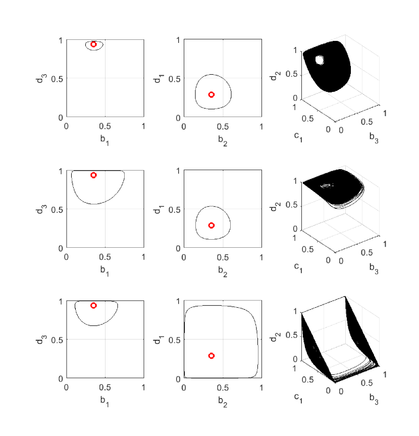
In this case, Solution 9 has a seven dimensional centre manifold with six purely imaginary eigenvalues, and a zero eigenvalue associated with the indeterminacy in c1subscript𝑐1c_{1} and d2subscript𝑑2d_{2} (see (16)). As shown in FigureΒ 13, b1subscript𝑏1b_{1} and d3subscript𝑑3d_{3}, and b2subscript𝑏2b_{2} and d1subscript𝑑1d_{1} behave periodically. The remaining frequencies, b3subscript𝑏3b_{3}, c1subscript𝑐1c_{1} and d2subscript𝑑2d_{2}, which are associated with Player 3 bluffing and Players 1 and 2 calling, have a long, close to periodic transient, but are eventually attracted to the boundary of the phase space. For P>5𝑃5P>5, qualitatively similar behaviour occurs around Solution 10.
Refer to caption
Figure 13: Periodic and close to periodic behaviour when P=4.65𝑃4.65P=4.65. The red circles indicate the location of Solution 9.

In each case, we can also calculate each Player’s profit, pisubscript𝑝𝑖p_{i}, by solving

d​pid​t=Ei,𝑑subscript𝑝𝑖𝑑𝑑subscript𝐸𝑖\frac{dp_{i}}{dt}=E_{i},

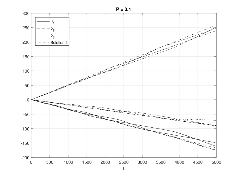
with the expected profit per game Eisubscript𝐸𝑖E_{i} given by (1) to (3). In each of the cases discussed above, each Player’s profit remains close to that given by the Lyapunov stable equilibrium solution if one exists, close to Solution 2 for 3<P<P33𝑃subscript𝑃33<P<P_{3} and close to Solution 7 for 4<P<P84𝑃subscript𝑃84<P<P_{8}. Even when the solution has a chaotic transient, as shown in FigureΒ 8, the profits pisubscript𝑝𝑖p_{i} shown in FigureΒ 14 for these three solutions, closely match the profits associated with Solution 2.
Refer to caption
Figure 14: The profits associated with the three solutions for P=3.1𝑃3.1P=3.1 shown in FigureΒ 8, along with the profit associated with Solution 2.

5 Conclusions

In this paper we studied a simplified version of three player Kuhn poker, [5], in which the card J is only in the deck so that there are more cards than players, making the game nontrivial. Each player must decide whether to bet with A, whether to bluff with Q and whether to catch bluffs with K. This leads to eleven nontrivial betting frequencies. We found that there are three ranges of values of the pot size, P𝑃P, for which there are three equilibrium solutions. The full structure of the equilibrium solutions was found using the computer algebra package, Mathematica.

We also studied an ordinary differential equation model of repeated play of the game, in which each player controls their own betting frequencies and tries to increase the rate at which they increase their profit, assuming perfect knowledge of all betting frequencies of every player. Our study of an even simpler game, [1], suggests that this gives some insight into the dynamics of repeated play provided that the players adjust their betting frequencies sufficiently slowly, and do not remember the play of the game for too long. We found that the betting frequencies never asymptote to one of the equilibrium solutions, and that the qualitative nature of the solutions depends on the pot size in a manner that is not at all intuitive. Periodic solutions, close to periodic solutions, and solutions with a long chaotic transient are all possible. This illustrates the fact that repeated three player poker games, even games as simple as the one studied here, can have very complex dynamics when the players try to maximise their profit over repeated play of the game, and concepts of balance and equilibrium, much studied by modern professional poker players (referred to as ’GTO’ play, [2]), may not be as relevant as they think in games with more than two players (but see also [3]).

Finally, we also note that the underlying idea of our ordinary differential equation model, namely that players try to maximise their profits, does not take into account the possibility of cooperation and alliances forming between the players. Although explicit collusion is banned in real world poker games, implicit collusion, in which the players signal to each other within the rules of the game, and no profit is shared outside the game, can occur, and may have a part to play in games such as the one studied in this paper. For an example of how this works in another three player game, see [4].

References

  • [1] John Billingham. Simplified three player Kuhn poker, 2017, arXiv:1704.08124.
  • [2] Doug Polk. GTO vs Exploitative Play: Which is the Better Strategy? https://www.youtube.com/watch?v=diNJ2gY2n7Q. Accessed: 2017-05-26.
  • [3] Alex Sutherland. GTO Poker outside of Heads Up - What it solves and what it does not. http://blog.gtorangebuilder.com/2014/03/gto-poker-outside-of-heads-up-what-it.html. Accessed: 2017-06-12.
  • [4] AdamΒ M. Sykulski, Archie Chapman, Enrique Munoz de Cote, and NicholasΒ R. Jennings. Ea2: The winning strategy for the inaugural lemonade stand game tournament. In Proceedings of the 2010 European Conference on Artificial Intelligence (ECAI), pages 209–214, 2010.
  • [5] Duane Szafron, Richard Gibson, and Nathan Sturtevant. A parameterized family of equilibrium profiles for three-player Kuhn poker. In Proceedings of the 2013 International Conference on Autonomous Agents and Multi-agent Systems, AAMAS ’13, pages 247–254, Richland, SC, 2013. International Foundation for Autonomous Agents and Multiagent Systems.