A SITELLE view of M31’s central region – I: Calibrations and radial velocity catalogue of nearly 800 emission-line point-like sources

Abstract

We present a detailed description of the wavelength, astrometric and photometric calibration plan for SITELLE, the imaging Fourier transform spectrometer attached to the Canada-France-Hawaii telescope, based on observations of a red (647 - 685 nm) data cube of the central region (11${}^{\prime}\times 11^{\prime}$) of M 31. The first application, presented in this paper, is a radial-velocity catalogue (with uncertainties of $\sim 2-6$ km/s) of nearly 800 emission-line point-like sources, including $\sim$ 450 new discoveries. Most of the sources are likely planetary nebulae, although we also detect five novae (having erupted in the first 8 months of 2016) and one new supernova remnant candidate.

1 Introduction

Aiming at characterizing the nearest liner, at the core of M 31, by studying line ratios and kinematics of the diffuse gas surrounding it (Melchior et al., in preparation), we have obtained a medium resolution (R $\sim$ 5000) data cube in the H$\alpha$–[N ii]–[S ii] range (649–684 nm) of a large section around the galaxy nucleus with the imaging Fourier transform spectrometer (iFTS) SITELLE.

This instrument, described in Baril et al. (2016); Drissen et al. (2010); Grandmont et al. (2012); Drissen et al. (in prep.), consists of a Michelson interferometer inserted into the collimated beam of an astronomical camera system, equipped with two fast-readout, low noise, deep depletion e2v CCD detectors ($2048\times 2048$, $0.32^{\prime\prime}$ pixels) providing a total field of view of $11^{\prime}\times 11^{\prime}$. The spectral range of a given data cube is selected by inserting the desired filter, chosen from a list covering the entire visible range, from 350 nm to 850 nm, in front of the collimator. SITELLE’s spectral resolution is very flexible, ranging from R = 1 (panchromatic) to R = 20 000. Details on data acquisition, and the process of transforming the two initial interferometric cubes into a single, calibrated spectral cube, are presented below.

The detection of several hundred H$\alpha$-emitting point sources in our M31 cube, some of which being new discoveries, has motivated the creation of a catalogue and, for this purpose, a significant improvement of the calibration methods used for SITELLE’s first data release (Martin & Drissen 2016, Martin et al. in preparation).

After a brief description of the instrument and the observations, Section 2 of this paper describes in details the wavelength, astrometric, and flux calibration of SITELLE data. Section 3 presents the method used to detect the H$\alpha$-emitting point sources before introducing the catalogue and a comparison with previous work based on narrow-band imagery and multi-object dispersive spectroscopy.

2 Observations and Data Calibration

2.1 Observations

The data cube was obtained on August 24, 2016, with SITELLE attached to the Canada-France-Hawaii telescope, and the SN3 filter (647–685 nm), designed to detect the H$\alpha$ line as well as the [N ii] 6548, 6584 and [S ii] 6717,6731 doublets in Milky Way H ii regions and nearby galaxies up to z=0.017. Parameters of the observations are listed in Table 1. The duration of the cube was 4.1 hours, including the 3.8-s overhead per step (CCD readout and mirror displacement and stabilization) giving a total on-source exposure time of 3.2 hours; sky was photometric and the median seeing, $0.9\,\arcsec$, was well sampled by the $0.32\,\arcsec$ CCDs attached to both output ports of the interferometer. The target resolution was 5000 on the interferometer axis giving a resolution of 4900 at the center of the field of view (at an incident angle of 15.4^∘). As we have not measured emission lines with a broadening significantly smaller than $\sim$20 km s^-1, we consider that this may be due to a loss of resolution of 1.7 %, i.e. an effective resolution of 4800. The data has been reduced with ORBS (Martin et al., 2012, 2015; Martin, 2015). Wavelength calibration has been performed with a method developed for ORCS (Martin et al., 2015) and described in details in section 2.2.1.

Although SITELLE was designed to reach higher spectral resolutions and that we have demonstrated that it can also reach this resolution during Commissioning and Science verification phases (Drissen et al., in prep.), this is only the second time that such a long scan has been obtained with the instrument. It was therefore an ideal opportunity to improve SITELLE’s calibration routine and compare our data with independent studies, all the more so that a large number of H$\alpha$-emitting point sources, most of which had previously published coordinates and radial velocities, were easily detected in the cube.

Table 1: Observation parameters of M 31. R is the effective resolution measured at the center of the data cube at the wavelength of H$\alpha$.

Filter	Exposure	Folding	Step	Step	ZPD	R
	time/step	order	size	nb.
SN3	13.7 s	8	2943 nm	840	168	4800

2.2 Wavelength calibration

SITELLE’s observation method is described in detail in Drissen et al. 2010 and Martin et al. 2016. An interferometric cube is obtained by moving one of the interferometer’s mirrors, while keeping the other one at a fixed position. The optical path difference (OPD) between the two interfering beams thus changes and modulates the intensity measured at the output port of the interferometer.

SITELLE is based on an off-axis interferometer configuration in order to collect the entire flux from the source from the combination of two complementary output ports instead of one in the classical Michelson configuration. The center of the field of view is thus 15.5^o away from the interferometer axis. On an interferometric image, each pixel measures the flux at a given incident angle $\theta$, with respect to the interferometer axis where $\theta=0$. Because of the off-axis configuration, $\theta$ varies between 11.8^o and 19.6^o (Fig. 1).

During a scan, the moving mirror is moved away from its original position, the Zero Path Difference (ZPD), where the OPD is null, by steps of equal size. At each step, an interferometric image is recorded on each output port with two 2k$\times$2k deep-depletion e2v CCD detectors (named Cam1 and Cam2). The image recorded on Cam2 is aligned with the image on Cam1 and both images are combined during the reduction process.

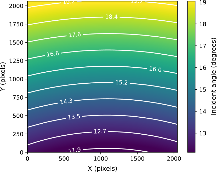
Figure 1: Incident angle ($\theta$) in the interferometer at each pixel. This angle was determined from the central wavelength of a HeNe (543 nm) laser as measured in SITELLE with a high resolution data cube; it varies between 11.8^∘ and 19.6^∘. The “observed” wavelength of the laser thus varies between  555 nm (543 nm / cos[11.8^∘]) and  576 nm (543 nm / cos[19.6^∘]).

When the interferogram recorded by one pixel is Fourier transformed to a spectrum, the knowledge of the exact incident angle is enough to produce the absolute wavelength calibration (Martin & Drissen 2016, Martin et al. in preparation). Indeed, as long as the interferogram is equally sampled, there is no uncertainty on the relative wavelength calibration. This assertion holds if the distribution of the sampling error has a mean of zero and its standard deviation is much smaller than the step size (Martin et al. in preparation). With SITELLE, wavelength calibration relies on a high resolution cube of a laser source obtained with the telescope pointing at zenith. The laser source is a green He-Ne laser at 543.5 nm. The exact wavelength of the laser is not very well known and is subject to drift with time. The absolute calibration of the whole cube is thus subject to a systematic bias but the relative, pixel-to-pixel, calibration is not affected. However, the relative calibration will show some distortions from a perfect model due to aberrations and deformations in the optical structure.

Even though a lot of efforts have been put on its robustness to temperature variations and changes of the direction of the gravity vector, the structure is still not ideal. By obtaining laser cubes in different directions with a zenithal angle of 47 ^∘ (corresponding to an airmass of 1.5), we have assessed during SITELLE’s commissioning, that the deformation of the optical structure could lead to relative velocity errors of up to 15 km s^-1, depending on the location of the target in the sky. The difference between the mean direction of the observed target and the zenith calibration laser cube being always smaller than 47 ^∘, the errors on the velocity measurements are expected to be less than 15 km s^-1, even with this basic calibration procedure. It is possible to refine this calibration by measuring the velocity of the night sky emission lines, when present in the filter bandpass. In particular, the SN3 filter (647 – 685 nm), which has so far been used to obtain the highest spectral resolution cubes with SITELLE, includes numerous Meinel OH bands. We have implemented a method in ORCS, SITELLE’s dedicated data analysis software, (Martin et al., 2015) to compute a map of the sky lines velocity in the field of view which has already been used to improve the wavelength calibration of other data sets (Martin et al., 2016; Shara et al., 2016). We have refined this method to calibrate the data obtained on M 31. Details are provided in the next section.

2.2.1 Method

Up to now, measuring sky lines velocity has proven to be the best way to calibrate a cube, both relatively and absolutely, regardless of the initial wavelength calibration. But this method has always been used on spectral cubes where the sky lines are detected with a decent SNR over the whole field of view. In those cases, sky spectra are extracted everywhere in the field and, eventually, a bi-spline model is fitted to interpolate the velocity at each pixel of the cube (see section 2.2.3).

However, in the case of M 31, the high level of continuum near the center of the object enhanced by the multiplex disadvantage of the FTS technique (Drissen et al., 2012; Drissen et al., 2014; Maillard et al., 2013), combined with the short exposure time per step, strongly reduces the SNR and prevents any precise ($\leq 2$ km/s) measurement of the sky lines centroid in the center of the field of view (FOV). Nevertheless, on the border of the FOV, the level of continuum is low enough to provide accurate measurements of the sky lines velocity (see Figure 4). Since the wavelength calibration is strongly tied to the optical structure of the interferometer, we can model the wavelength calibration map from a small set of instrumental parameters and fit the known velocity points (i.e. on the border of the FOV) to estimate the velocity where no reliable measure of the sky lines can be made (i.e. at the center FOV). It is then possible to compute the correct wavelength calibration everywhere in the FOV with precision.

This improved calibration method involves:

1. Computation of a set of initial parameters from the calibration laser map measured at zenith;

2. Measurement of the velocity of the sky lines, which translates directly into a wavelength calibration error since this velocity must be 0;

3. Modeling of a new calibration laser map with a new set of parameters which fit the measured velocity of the sky lines.

We will now describe the model of the calibration laser map we have developed to relate the deformation of the optical structure to the value of the incident angle at each pixel of the FOV. Note that the calibration laser map is taken at zenith. The fit of this calibration laser map with the model permits to define an initial set of parameters which can eventually be changed to model what would be the real calibration laser map in the direction of the target (here M 31).

2.2.2 Calibration laser map modelling

The best way to fit a calibration laser map is to construct a model $M$ defined as a function of instrumental parameters $p$, which permits to calculate $\sigma$, the measured laser wavenumber related to the wavelength $\lambda$ via $\sigma=1/\lambda$, at any given pixel position ($x$, $y$).

$$\sigma(x,y)=M(x,y,p)\;,$$ (1)

Recalling that the angle between the interferometer axis and the detector pixel is $\theta$, we can start by providing the relation between the measured velocity error $\epsilon_{v}$ and the error $\epsilon_{\theta}$ made on the calculated value of the incident angle $\theta$. Indeed, following the equation 29, any error on $\theta$ translates into an error on the measured wavenumber, $\sigma$, with respect to the real wavenumber $\sigma_{0}$,

$$\sigma=\frac{\sigma_{0}}{\cos(\theta+\epsilon_{\theta})}\;.$$ (2)

This error will in turn result in an error on the measured velocity,

$$\epsilon_{v}=c\left(\frac{1}{\cos(\theta+\epsilon_{\theta})}-\frac{1}{\cos(\theta)}\right)\;,$$ (3)

where $c$ is the speed of light.

If the optics in front of the detector are not taken into account, i.e. the computed distances are not corrected for the optical magnification, an idealized structural model can be deduced from simple geometrical considerations (the optics and the detector are also considered distortion free). The detector is considered as a perfect plane perpendicular to the direction of the incoming beam at a distance $d$ from the beamsplitter. Projected into spherical coordinates, as shown in Fig. 2, this angle is defined by its longitude $\lambda$ and its latitude $\varphi$. The angles that define the direction from the origin to the center of the detector (the detector axis) are $\lambda_{\text{c}}$ and $\varphi_{\text{c}}$.

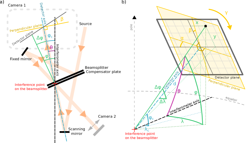
Figure 2: Idealized model of the interferometer structure. a) 2D projection of the whole interferometer structure. The off-axis configuration, with a beamsplitter tilted with respect to the classical 45^∘ configuration, appears clearly. Some of the indications shown in the complete 3D figure (b) are reported. The nominal incident angle $\theta$ at the center of the detector is 15.5^∘. By projection the angles $\theta$ and $\varphi$ seem to be the same but they are not. Note that the optics of the cameras, in front of the detector plane, are not taken into account in the model. b) 3D representation of the model of the interferometer. The equator plane (or reference plane) and the pole direction of the spherical coordinates system are indicated in grey. The origin is the point on the beamsplitter where the detector axis crosses the semi-transparent coating.

To calculate the incident angle of any pixel on the detector, one can first determine the angles $\Delta\lambda$ and $\Delta\varphi$ of this pixel with respect to the detector axis (the direction which points from the origin to the center of the detector). Since the physical size of the pixel $p$ is known (15 $\mu$m), the physical position of a pixel on the detector ($x$, $y$) can be simply related to its index ($i_{x}$, $i_{y}$)

$$x=p\,i_{x}$$ (4)

$$y=p\,i_{y}$$ (5)

The rotation of the detector by an angle $\gamma$ can be taken into account with a rotation matrix

$$x=p\,i_{x}\cos(\gamma)+p\,i_{y}\sin(\gamma)$$ (6)

$$y=p\,i_{y}\cos(\gamma)-p\,i_{x}\sin(\gamma)$$ (7)

The plane of the detector can also be tilted with respect to the plane perpendicular to the detector axis (tip-tilt angles $\alpha$ and $\beta$). The angle $\Delta\lambda$ and $\Delta\varphi$ are computed with the classical tangent law

$$\Delta\lambda=\arctan\left(\frac{x-d}{x+d}\frac{1}{\tan(0.5(\alpha+\pi/2))}\right)-\frac{\alpha}{2}+\frac{\pi}{4}$$ (8)

$$\Delta\varphi=\arctan\left(\frac{y-d}{y+d}\frac{1}{\tan(0.5(\beta+\pi/2))}\right)-\frac{\beta}{2}+\frac{\pi}{4}$$ (9)

The direction of the pixel with respect to the interferometer axis is thus

$$\lambda=\lambda_{c}+\Delta\lambda$$ (10)

$$\varphi=\varphi_{c}+\Delta\varphi$$ (11)

and the incident angle $\theta$ can finally be derived with Vincenty’s formula (Vincenty, 1975),

$$\theta=\arctan\left(\frac{\sqrt{(\cos(\varphi)\sin(\lambda))^{2}+\sin(\varphi)^{2}}}{\cos(\varphi)\cos(\lambda)}\right)\;.$$ (12)

Finally, from equation 25, we can compute the measured wavenumber of the laser source of nominal wavenumber $\sigma_{0}$ at a given incident angle $\theta$ (we recall the equation here for clarity)

$$\sigma_{\theta}=\sigma_{0}\cos(\theta)\;.$$ (13)

This model provides a good description of the measurement of the incident angle that can be done via the observation of a calibrated laser source. If we look at the typical values of the parameters returned by a fit of an arbitrary calibration laser map we find a distance $d$ of $\sim$23.5 cm (depending on the chosen wavelength of the calibration laser), which, magnified by 3.3 (the magnification of the camera optics), gives a real distance of $\sim$76 cm: a few centimeters larger than the real distance from the dielectric coating to the detector surface. Tip-tilt angles are also generally small which appears mechanically correct.

However,this model does not take into account the distortions produced by the optics which slightly changes the position where the light at a given incident angle is measured on the detector (see Fig. 3).

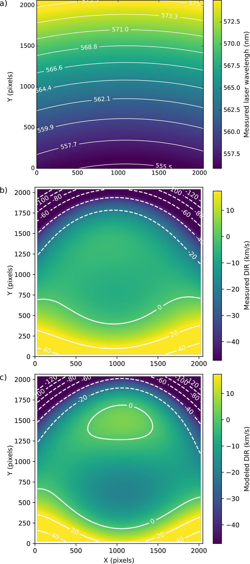
Figure 3: a) Calibration laser map. The real wavelength of the calibration laser is 543.5 nm. The measured wavelength depends on the incident angle $\theta$ of the incoming light with respect to the interferometer axis (see Fig. 1). b) Distortion Induced Residual once the structural model is subtracted. The wavelength error is given in terms of velocity error at H$\alpha$. c) Modeled DIR computed with the astrometric distortion model. Contours are solid when the value is positive and dashed when negative.

If we assume that our model is correct in first approximation, the residual from the fit on the measured calibration laser map must come from optical aberrations, such as distortions and wavefront errors, with some normally distributed noise, $\mathcal{N}$, that can be reduced by fitting the residual with an appropriate model (Zernike polynomials in this case), i.e., from equation 1:

$$\sigma_{\text{observed}}(x,y)=M(x,y,p)+DIR(x,y)+\mathcal{N}\;,$$ (14)

DIR$(x,y)$ being the Distortion Induced Residual, as the optical distortions are a major contributor to this residual. Indeed, we can use the distortion model obtained from the astrometric calibration (see section 2.3) and try to model what would be the observed DIR (see Fig. 3). We can see that, even if small features are not perfectly reproduced, most of the measured DIR can be explained by optical distortions, especially in the corners. Note also that we are using a distortion model calculated in the red part of the spectrum (the SN3 filter is centered at 666 nm) while the calibration laser map is observed at 543.5 nm and that distortions are likely to be chromatic. A more careful study of the relation between the residual and the astrometric distortion pattern still needs to be done but is beyond the scope of this paper.

The idea that a complete model of the calibration map is the sum of a geometrical model of the interferometer that changes with the direction of the gravity vector plus a constant DIR (see equation 14) is confirmed by the comparison of the DIRs computed from the fit of 5 calibrations laser maps obtained at different telescope pointings. During the commissioning, 4 calibration laser maps have been obtained at an angle of 47 ^∘ in 4 different directions (north, south, east, west). They have been compared with a calibration laser map obtained at zenith. We have found that the difference between the DIRs computed with the fit of each of these 5 calibration laser maps was always smaller than 1 km s^-1. However, the difference between the geometrical models $M(x,y,p)$ can reach 20 km s^-1. Note that the final residual made on each fit (which, from equation 14, must be noise only) is a perfect Gaussian distribution with a standard deviation of 0.5 km s^-1. We conclude that, as long as the optics are not changed, the DIR remains stable and the real calibration map of a target observed in a direction different from the zenith only depends on the instrumental parameters $p$ of the geometrical model $M(x,y,p)$. Note that a standard deviation of 0.5 km s^-1 on the fit of the calibration laser map does not mean that our precision on the wavelength calibration will be the same. This result better gives a lower limit on the calibration precision. The wavelength calibration of the actual data is discussed in the next section.

2.2.3 Fit of the sky velocity

We have measured the velocity of the sky lines over the whole field of view by extracting 1600 spectra at each point of a 40$\times$40 grid. Each sky spectrum was integrated over a 30$\times$30 pixels box to improve its signal-to-noise ratio. But, as explained in section 2.2.1 the high level of continuum near the center of the galaxy prevents any precise measure over a large part around the center of the field (see Fig. 4). We have thus used the model described in the previous section to compute the real instrumental parameters during the observation of M 31 by fitting our model to the measured velocity of the sky lines (Table 2). Note that the rotation angle has been fixed at 0 because there is a strong degeneracy between the rotation angle and $\varphi_{c}$ which leads to unphysical values of the structural parameters without giving an appreciable difference in the precision of the fit.

With this method we have been able to estimate the sky lines velocity in the central region of the field of view where no sky lines could be measured and reduce the initial velocity gradient of more than 15 km s^-1 (Fig. 4) down to a much flatter error with a standard deviation of 2.21 km s^-1 (Fig. 5). This is considered to be our systematic uncertainty and has been added to all the estimations of the uncertainty on the velocity measurements.

Nevertheless we must admit that, the standard deviation is still higher than the 0.5 km s^-1 obtained with the direct fit of the calibration laser map (see section 2.2.2). We see two possibilities regarding the accuracy of the DIR. First, the stability of the DIR, which is not recomputed (only the instrumental parameters can be fitted), is ensured as long as the optics are not touched. Sadly, no calibration laser cube has been taken during the night of the observation, which was the first night of the run. The next night, one of the two cameras (Cam1) was removed to perform some tests and was put back in place but with a rotation of 0.8 ^∘ (this rotation corresponds to the angle $\theta$ in the model described in section 2.2.2), making the measurement of the DIR from the calibration laser, obtained after the changes on Cam1, much less precise. We have tried to simulate the real calibration laser map (and thus the real DIR) at the date when M 31 was observed by rotating Cam1 on the calibration data obtained a few days after with no real success. That’s why, even if this possibility cannot be discarded, we do not believe that the difference we see is due to the camera change. The other possibility comes from the fact that our model has only been tested with green laser cubes (543.5 nm) and it is possible that the DIR calculated at 543.5 nm may not be exactly the same in the SN3 filter (i.e. around 660 nm). If we consider that a deviation of 1 pixel in the distortion pattern can account for up to 6 km s^-1, small variations of the refractive index of the beamsplitter could explain why the error is structured and has a higher than expected standard deviation (Fig. 5).

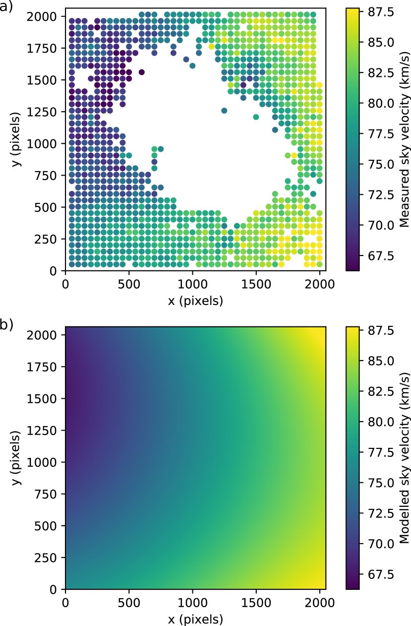
Figure 4: a) Measured velocity of the sky lines in the SN3 filter on integrated spectra of 30$\times$30 pixels in SITELLE’s field of view. The points where no sky lines could be measured and the points having an uncertainty greater than 1.7 km s^-1are not displayed (and were not used for the fit). The white area (depopulated from reliable measurements) corresponds to the central region, where the continuum flux is very high. The main goal of the fitted model shown below is to give an estimate of the sky velocity in this area (b) b) Velocity model of the sky lines computed from the calibration laser map model and fitted over the velocity points shown in (a). Fitted parameters of the model are reported in Table 2 and residuals of the fit are shown in Figure 5.

Table 2: Fitted parameters of the calibration laser map model for the wavelength calibration of M 31 based on the measured sky lines velocity. The reference camera is Cam1.

Beamplitter-detector distance($d$)	23.8 cm
X angle from the optical axis to the center($\lambda_{c}$)	-0.47 ∘
Y angle from the optical axis to the center($\varphi_{c}$)	15.44 ∘
Tip-tilt angle of the detector along X ($\alpha$)	0.25 ∘
Tip-tilt angle of the detector along Y ($\beta$)	-0.43 ∘
Rotation angle of the detector ($\gamma$)	0 ∘ (fixed)
Calibration laser wavelength	543.37 nm

Figure 5: a) Map of the residual error on the velocity calibration after the computed model is removed. b) Histogram of the residual error on the velocity calibration corresponding to the map presented above. The median of the distribution is 0.25 km s^-1 and its standard deviation is 2.21 km s^-1. This systematic uncertainty has been added to all velocity measurements.

2.3 Astrometric calibration

The astrometric calibration model can be divided into three levels of refinement. The first level starts with the determination of 5 general registration parameters: the target coordinates in the image, its celestial coordinates and the angle between the image’s Y axis and the North. This rough model is arguably more precise near the center of the frame, where the effects of the optical distortions are minimal. Indeed, the second level includes a distortion model based on the Simple Image Polynomial (SIP) convention (Hook et al., 2008). All the parameters estimated for the first and the second levels of astrometric calibration can be written into any FITS header (Hanisch et al., 2001) and interpreted with most FITS viewers (e.g. SAO Image DS9). But, even with a SIP distortion model, the calibration error can be as large as 1.5 ″in the corners of the image (Fig. 6 and Fig. 7). The third level of refinement relies on two distortion maps (one for each axis of the image) which are computed from the residual between the SIP calibration model and the real position of the stars in the image; an error on the calibration smaller than 0.3 ″(1 image pixel) is then reached. While the first level only requires a few stars to get an acceptable calibration, the other two require the observation of a densely populated star field to precisely determine the distortion model.

2.3.1 First level: general registration parameters

The coordinates at the center of the field of view are generally known with an uncertainty smaller than 15 ″and the rotation angle cannot vary by more than 5 ^∘. Many optical modifications between each run since SITELLE’s commissioning explain this large uncertainty on the rotation angle from one observation to another; these are expected to be much less numerous from now on. Nevertheless, a good and robust estimate of the general parameters is obtained with a two step registration process.

1. A first reduction of the uncertainty is made from the correlation of the 2D histogram of the real list of positions of all the stars visible in the image and the positions of the stars found in a catalogue. In the case of M 31, we have used the Gaia DR1 catalogue(Gaia Collaboration et al., 2016a, b). With this method, the two lists do not need to contain exactly the same stars. The peak of the correlation image will provide the shift between both lists with an uncertainty which depends on the size of the 2D histogram bins (generally of the order of 10 pixels, i.e. 3 ″). Note that a brute force search, which consists in a systematic search along a range of possible angles, must first be used to find the rotation angle that maximizes the amplitude of the histogram peak.

2. A brute force method, which consists in a systematic search through all the possible sets of parameters – each parameter being explored over a given range of possible values, is used to find the set of parameters which maximizes the total flux measured in the image at the positions projected from the catalogue. When a maximum of stars are present at those positions the total flux is a its highest.

2.3.2 Second level: SIP distortion model

Once the general registration parameters are known, it is possible to match the position projected from a catalogue with the stars on the image, especially near the center where the error is less than a few pixels. The parameters of a fourth order SIP distortion model are found with a least-square Levenberg-Marquardt minimization algorithm (Levenberg, 1944; Marquardt, 1963) to reduce as much as possible the distance between both lists (which now must contain the same stars). As the number of suitable stars in M 31’s central region is small, we have used an image of a field in NGC 6960, obtained the same night, to compute the SIP parameters.

2.3.3 Third level: residual distortion maps

Even if the SIP model performs remarkably well at describing the distortions of the field of view, the error can be as large as 1.5 ″, especially in the corners of the field where distortions are the strongest (Fig. 6). Primarily because of SITELLE’s optics which aberrations are radially dependant and secondarily because of the image quality which is severely degraded in the corners for reasons still unknown. To reduce this error down to less than one pixel, we have no choice but to compute two distortion maps, one for each axis (shown on Fig. 8). The interpolation of the displacement along both axes between the stars is modelled with Zernike polynomials which are well suited to model wavefront distortions.

The resulting calibration must have a precision better than one pixel (0.32 ″), everywhere in the field. It seems difficult to compare with other catalogues since the catalogue we use (Gaia DR1) is, by far, the one which contains the more stars with the highest precision. A comparison of our catalogue of emission-line point-like sources (see section 3) with another catalogue is made in section 3.4. It suggests an upper-limit uncertainty of 0.21 ″on our calibration which supports our calibration.

Figure 6: a) Histogram of the position error after the first calibration level. The median of the error is around 2 ″and can be as large as 14 ″in the corners of the image. b) Histogram of the position error after the second calibration level. The median of the error is now smaller than 0.3 ″which is more than 6 times better than the first level median error. The histograms of the stars in the corners, defined as having a radius with respect to the center of the field greater than 1000 pixels, i.e. 5.35 ′, are shown in blue. The cumulative histograms are shown in light grey.

Figure 7: Position error in one region of the field of view of M 31 taken far from the center where the distortions are the most important. The crosses indicate the computed position of the stars after the first calibration step, in red, the second calibration step, in orange, and the third calibration step, in green.

Figure 8: Residual distortion maps along the Y (a) and X (b) axes used for the third level of astrometric calibration. The position error is given in pixels. One pixel has a dimension of 0.32 ″.

2.4 Flux calibration

The flux calibration was performed from two calibration sources: 1) The spectrum of the spectrophotometric standard star GD71 (Bohlin, 2003), obtained in January 2016, which is used to eliminate as much as possible any strong wavelength dependence ; 2) the median combination of a set of 10 images of the standard star HZ 4 (Bohlin et al., 2001) obtained right after the end of the cube observation with photometric conditions similar to the observation conditions. The exact value of the interferometer’s modulation efficiency (ME), which acts essentially as an additional throughput loss, is the major source of uncertainty on the absolute flux calibration Martin & Drissen (2016). Interferometric images of the laser source have been obtained before and after the observation of the target in order to measure the variation of ME at the calibration laser wavelength (543.5 nm) with respect to its nominal value (85 %). We have measured a loss of 11.7 %. The initial flux calibration of M 31 in the SN3 filter has been corrected for this loss (thus multiplied by a factor 1.13). But given the possible uncertainty on this estimate, we have double-checked it using Hubble Space Telescope (HST) narrowband images of the target. The advantage of HST’s narrowband filters is that they can easily be simulated by integrating the spectral cube over the filter’s well-known transmission curve. As SITELLE’s cube flux is expressed in erg cm^-2 s^-1 Å^-1 and given the filter transmission curve $F(\sigma)$, the integrated flux $\tilde{\phi}_{F}$, expressed in erg cm^-2 s^-1 Å^-1, is

$$\tilde{\phi}_{F}=\frac{\int_{-\infty}^{+\infty}\phi(\sigma)F(\sigma)d\sigma}{\int_{-\infty}^{+\infty}F(\sigma)d\sigma}\;.$$ (15)

If one converts the flux in terms of surface brightness, expressed in erg cm^-2 s^-1 Å^-1 per HST pixel surface ($S_{\text{HSTCamera}}$), i.e.

$$\tilde{B}_{F}=\frac{\tilde{\phi}_{F}}{S_{\text{SITELLE}}}S_{\text{HSTCamera}}\;,$$ (16)

with $S_{\text{SITELLE}}=0.32^{2}$ arcsec², the image $\tilde{B}_{F}$, once properly aligned, can be directly compared with the HST frame. We have made this comparison for three different regions of the field of view (called WFC3, ACS1, ACS2, shown in Fig. 9) and four different filters (F656N, F658N, F665N, F660N). Histograms of the flux ratio between the integrated frames and the HST frames are presented in Fig. 10 and the first moments of their distributions are listed in Table 3.

2.4.1 Relative flux calibration

We can estimate the pixel-to-pixel relative uncertainty from the flux ratio maps. But we must be careful with the absolute calibration of the Hubble images. Indeed, the average sky background intensity reported in the WFC3 Instrument Handbook is $3.8\times 10^{-18}$ erg cm^-2 s^-1 Å^-1 arcsec^-2 at 6000 Å that must be compared to the surface brightness of M 31 which ranges in our field of view from $5\times 10^{-17}$ to $5\times 10^{-15}$erg cm^-2 s^-1 Å^-1 arcsec^-2 accounting for 1.4 % in the WFC3 field and around 7 % in the ACS fields. Also, from the WFC3 Instrument Handbook the quoted photometry accuracy is around 2–3%. This uncertainty alone is sufficient to explain the difference in the median ratio in the different fields especially the 7 % difference between the F656N filter and the F658N and F665N filters obtained in the same region at the center of the field. It is thus difficult to assert that there is no gradient in the absolute flux calibration smaller than 8 %. In the ACS fields a higher limit of 4 % on the relative calibration can be deduced from the standard deviation of the ratio histograms. In the central region the smaller standard deviation is around 2 % which sets the higher limit on the relative flux calibration in this region.

2.4.2 Absolute flux calibration

To get the most conservative estimate on the absolute flux calibration correction we have computed the mean of the 5 median values of the flux ratios (considered with their uncertainty) to obtain a mean flux ratio of $96.9\pm 1.4$ % which has been used to correct the flux calibration of our data.

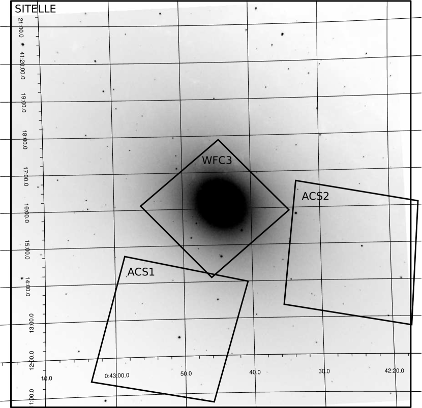
Figure 9: Positions of the HST fields over SITELLE’s field of view used to refine the flux calibration.

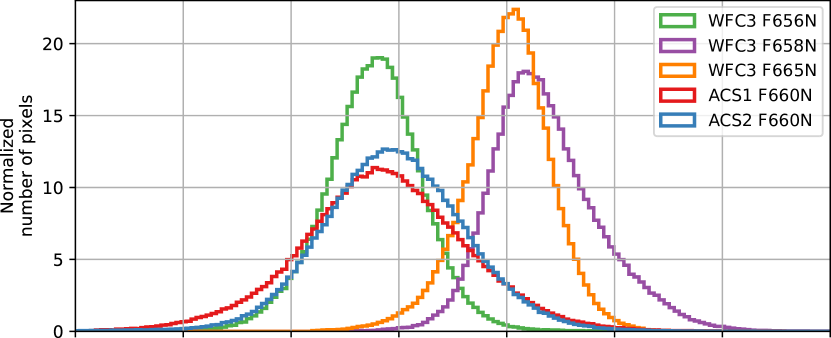
Figure 10: Histograms of the flux ratio between the integrated frames (which simulate HST frames) and the real HST frames. The median and standard deviation of theses distributions are reported in Table 3

Table 3: Median and standard deviation of the histograms of the flux ratios shown in Figure 10. $\lambda_{\text{mean}}$ is the pivot wavelength of the HST filters.

Instrument	Filter	$\lambda_{\text{mean}}$	Field	Median [Std]
		(in nm)		(in %)
WFC3 UVIS1	F656N	656.15	WFC3	93.8 [2.3]
WFC3 UVIS1	F658N	658.56	WFC3	101.5 [2.6]
WFC3 UVIS1	F665N	665.60	WFC3	100.1 [2.1]
ACS WFC	F660N	659.95	ACS1	94.3 [4.0]
ACS WFC	F660N	659.95	ACS2	94.7 [4.1]

3 Emission line sources near the center of M 31

While the main objective of the SN3 data cube was to study the diffuse gas around M31’s nucleus, we were delighted to see a very large number of point-like sources appearing as we scanned the reduced cube. Since the brightest of them could likely be used to assess the validity of our calibrations, we put some efforts into the systematic detection and characterization of point-like emission-line sources in this cube. The following section thus describes the detection technique, the catalogue resulting from this analysis and comparisons with previous catalogues, as well as a discussion of some interesting sources.

3.1 Source detection

The relatively large velocity range ($\sim 800$ km s^-1) due to galactic rotation near the center of M31 requires a dedicated algorithm to detect emission-line sources. We devised such an algorithm, which aims at detecting an excess of flux in at least one spectral channel for a given pixel with respect to its surroundings. First, the spectrum of this pixel is replaced by the median spectrum of the 3$\times$3 pixels box centered on it (matching the mean seeing during the observations). The median spectrum of a 9$\times$9 pixels box (excluding the central 3$\times$3 pixels) is then subtracted. The maximum flux of this background-subtracted spectrum is then stored in a detection map at the location of the pixel under investigation (see Fig. 11). This map, which therefore provides the level of emission of each pixel above its surrounding background, highlights numerous point sources, the brightest foreground stars and some very bright portions of the filaments of diffuse gas around the core of the galaxy. Finally we have checked this detection map by eye for the presence of point-like sources which spectra have been extracted and fitted manually.

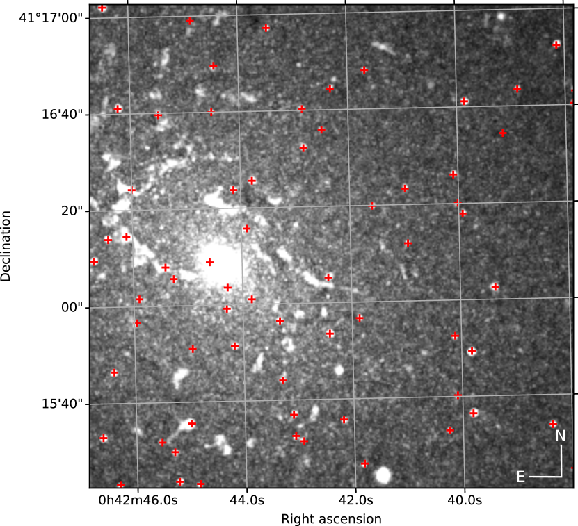
Figure 11: Cropped region of the detection frame around the center of M 31. Red crosses indicate the positions of the sources of the catalogue.

3.2 Extraction and fit of the sources

Once the identification of candidates was completed, the backround-subtracted spectrum of each candidate has been integrated in a 3$\times$3 pixels box around the central pixel. This time, the background spectrum was chosen to be the median spectrum of a 30$\times$30 pixels box (excluding the central 3$\times$3 box), which was found to be the optimal setting to maximize the signal-to-noise in the whole galaxy though it might not be optimal near the very center of M 31 where there is an important background gradient.

The spectrum was then fitted with a model made of 5 emission lines (H$\alpha$, [N ii] $\lambda 6548$, [N ii] $\lambda 6584$, [S ii] $\lambda 6717$, [S ii] $\lambda 6731$) plus a flat background. Note that the HeI $\lambda 6678$ line was not detected anywhere. The analytic model describing the line spread function of the emission lines is the convolution of a sinc, the instrumental line shape, and a Gaussian, an approximation of the real line shape (see Fig. 12). The line model, described in details in Martin et al. (2016), has 3 varying parameters: amplitude, velocity and broadening of the Gaussian; the FWHM of the sinc line is known and fixed as it depends only on the maximum OPD of the interferogram (see equation 5 of Martin et al. 2016). All the 5 emission lines were considered to share the same velocity and the same broadening.

We have chosen to integrate the source spectrum into a 3$\times$3 box in order to maximize the signal-to-noise ratio of our spectrum. But the PSF clearly extends beyond this limit, so the flux must be corrected for this aperture loss. We have simulated our integration model on a synthetic star with a Moffat point spread function (Moffat, 1969). The real center of the synthetic star was randomly positioned, with a uniform distribution, in the central pixel to mimic the fact that the real center of the integrated source can be anywhere in the central pixel of the 3$\times$3 box. The shape parameters of the synthetic star (width and the Moffat parameter $\beta$) were taken from a fit of multiple stars in the deep frame of the cube (the deep frame represents the integral of the cube along the spectral axis). From the analysis of 100 000 trials we can conclude that the measured flux must be multiplied by 1.88 $\pm 0.07$.

The final correction made on the measured flux is the product of the modulation efficiency loss, the flux calibration obtained from the comparison with Hubble images and the computed PSF loss which gives a final correction factor FC:

$$\text{FC}=1.13\,\times\frac{1}{0.969\pm 0.014}\,\times 1.88\pm 0.07=2.199\pm 0.088\;.$$ (17)

The systematic relative uncertainty made on the measured flux, independently of the uncertainty due to the SNR of the fitted spectra, is thus 4 %.

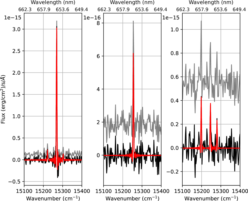
Figure 12: Examples of extracted spectra. The raw spectrum is in gray, the background corrected spectrum in black and the fit in red. Only the region around the H$\alpha$ line is shown.

3.3 Description of the catalogue

We have detected and catalogued a total of 797 H$\alpha$ emitting sources in our field of view (see Table 7). The radial velocity and the broadening of the lines as well as the flux of H$\alpha$, [N ii] $\lambda 6584$, and the combined flux of [S ii] $\lambda 6717$ and [S ii] $\lambda 6731$ have been reported in the catalogue with their corresponding uncertainty. When the SNR of a line was smaller than 5 and thus not clearly detected, we have reported an estimation of the upper limit of the flux. This upper limit was considered to be the minimum value between the estimated amplitude plus 3 times its uncertainty or 5 times the uncertainty. As the lines are modeled with the same velocity, the [S ii] and [N ii] lines are always present in the fit results but the amplitude uncertainty might be much higher than its measured value (as already mentioned a line was considered detected for a SNR higher than 5). In this case, the uncertainty used to calculate the upper limit on the [S ii] or the [N ii] flux is strongly related to the background noise.

Examples of spectra are shown in Figure 12. The reported SNR is the maximum intensity attained by the spectrum (i.e. by the H$\alpha$ or [N ii] $\lambda 6584$ line) corrected for the background and the median intensity and divided by the standard deviation of the residual of the fit (see section 3.2).

We have cross-matched our sources with the catalogues of Halliday et al. (2006) and Merrett et al. (2006), aimed at the detection and characterization of planetary nebulae specifically targeting the [O iii] $\lambda 5007$ line, and reported the corresponding ID in Table 7. We have detected 304 of the 332 sources detected in [O iii] by Merrett et al. (2006) (a 91.5% completeness) and 149 of the 154 sources observed by Halliday et al. (2006) a 96.8% completeness). A comparison of our measured velocity with the velocity reported by Halliday et al. (2006) is made in section 3.4.

Supernovae remnants and novae were detected but have been removed from the catalogue, the first ones because they are not point-like and the second ones because of their transient nature. They are discussed independently in section 3.6.

3.3.1 Luminosity function and completness

The luminosity function, uncorrected for extinction, of the sources in the catalogue is shown in Figure 13 and has been calculated with the relation

$$L_{H\alpha}=4\pi D^{2}F(H\alpha)\;,$$ (18)

$D$ being the distance to the center of M 31 assumed to be 0.783 Mpc (Mochejska et al., 1999).

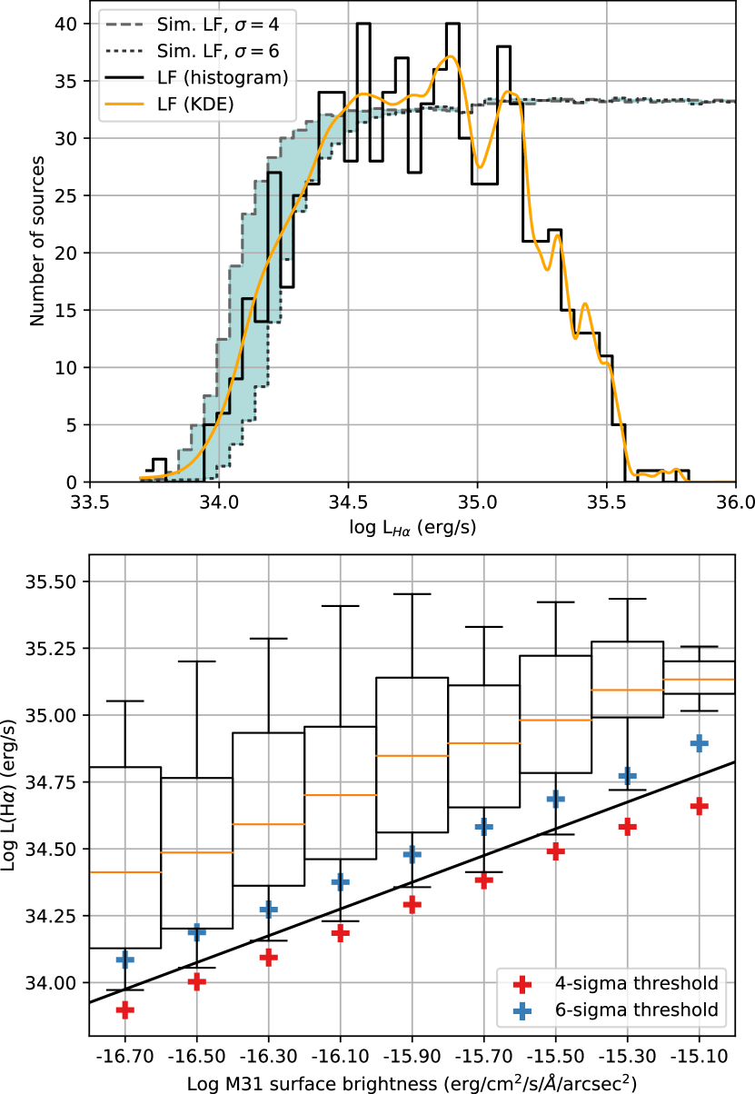
Figure 13: Top: H$\alpha$ luminosity function $L_{H\alpha}$ of the catalogued sources, uncorrected for extinction. The kernel density estimation (Rosenblatt, 1956; Parzen, 1962) of the luminosity function is also plotted as an orange line. The histograms simulated for a detection threshold at $4\sigma$ and $6\sigma$ are shown. The blue region between both simulated histograms indicates where the luminosity function should fall for a detection threshold between $4\sigma$ and $6\sigma$. Bottom: Simulated 90 %-completness (luminosity under which the completness is smaller that 90 %) with respect to the background flux for a detection threshold at $4\sigma$ and $6\sigma$. The function from equation 19 is drawn in solid black. The box and whiskers plot represents the distribution of the luminosity of the catalogued sources per bins of the underlying galaxy’s surface brightness. Whiskers are set at the 5th and 95th percentiles of the distributions.

Note that, from (Azimlu et al., 2011; Walterbos & Braun, 1992) maximum luminosity of planetary nebulae is $\sim 5\;10^{35}$ erg s^-1 which is the case of 99.6 % of our sources. Our detectability limit in terms of flux $F(H\alpha)$ is around $10^{-16}$ erg s^-1 with 4.1 hours of integration over the very bright background of M 31 which is certainly one of the worst case scenario for a Fourier transform spectrometer.

We have verified the completeness of our sample by simulating the detection of 10 million randomly positioned emission-line point-sources in one channel of a spectral cube. Considering only the photon noise contribution, the noise is the same in every channel and its amplitude is the square root of the total number of counts accumulated in each pixel (Drissen et al., 2012; Drissen et al., 2014; Maillard et al., 2013). Starting with a map of the total number of counts in each pixel we can add a group of randomly positioned sources with a log-uniform flux distribution and compute its square root to obtain a map of the photon noise. Each source has its flux concentrated in only one pixel and one channel which greatly simplify the simulation of the detection process. The noise is multiplied by $\sqrt{9}$ to simulate the 3$\times$3 binning used for the detection and the extraction of the spectra. The flux of the one-pixel star is divided by 1.88 to simulate the loss of flux in the wings of the point spread function. It is also divided by 1.25 to simulate the fact that its real flux is distributed as a sinc line spread function with a width of 1.25 channels . All the pixels showing a value above the background level plus a given number of times the calculated noise $\sigma$ are considered as detected sources. Note that the 10 millions sources were simulated by sets of a thousand sources in a SITELLE frame of 4 million pixels. So that the probability of having multiple sources at the same pixel is negligible. The histograms of the detected sources for a threshold at 4$\sigma$ and 6$\sigma$ are shown in Figure 13. They reproduce well the slope of the luminosity function at low luminosity level, confirming that the completeness is good at a detection threshold of $\sim 5\sigma$.

In terms of homogeneity of the completness in the field of view, it is clear that the level of detectability changes with the surface brightness of M 31. We have used the results of the simulation detailed above to compute the 90 %-completness (i.e. the limit luminosity under which the completness falls under 90 %) with respect to M 31’s surface brightness $B$ for a detection threshold of $4\sigma$ and $6\sigma$ (see Fig. 13). The function which best fits the mean of the simulated data is

$$\log(L_{\text{H$\alpha$}})=0.5\log(B)+42.325\;.$$ (19)

We have also reported in Figure 13 a box and whisker plot representing the distribution of the luminosity of the catalogued sources per bins of the underlying galaxy’s surface brightness. Whiskers are set at the 5th and 95th percentiles of the distributions. If we examine closely the whiskers corresponding to the 5th percentile of the luminosity distribution we can see that they nearly all fall between the $4\sigma$ and $6\sigma$ simulations, except for the highest brightness bin which contains much less sources than the others. This result confirms the adopted simulation process.

3.3.2 LGGS cross-match

Table 4: Results of the detection of our sources in the LGGS ratio frames when they are considered together and independently (see text for details). Detection is said non-applicable (N/A) when the source is situated in the saturated region near the centre of M 31 (in at least one of the frame when frames are considered together). A source is considered undetected in both frames if it is not detected in any of the frames and if it is not situated in a saturated region. A source is considered detected in both frames when it is detected in at least one of the frames.

LGGS ratio frame	detected	undetected	N/A
H$\alpha$/R	533	147	117
[O iii]/B	389	376	32
H$\alpha$/R or [O iii]/B	595	117	85

We have verified if our sources were also detectable in the images of the Local Group Galaxies Survey (LGGS, Massey et al. 2006; field F5). To do so, we have divided the narrowband images centered on H$\alpha$ and [O iii] $\lambda 5007$ by their corresponding broad-band images R and B and checked by eye if a source could be seen at the location of our emission-line sources. Note that a region of 2.5 arc-minutes and 15 arc-seconds at the center of M 31 in, respectively, the R and B images is saturated and cannot be studied; sources in this region are marked with “N/A” in the corresponding columns. We report in table 4 the number of detected and undetected sources in each ratio image. A total of 595 of our sources were detected in at least one of the LGGS ratio images while 117 were clearly not detected ; 85 are not detected in one of the frame but are situated in a saturated region in the other frame, in which case the non-detection is less clear. If, in most cases, those undetected sources have a relatively low SNR (which may explain the non-detection), with a median of 5, seven of them have a SNR larger than 7 and should have shown up in the LGGS ratio images. It indicates that they could display new or variable emission lines (the field F5 of the LGGS data has been obtained the 22th of September 2001). Another interesting fact is that all those objects share a similar spectral morphology, namely that they display a broad H$\alpha$ emission line (broader than the instrumental resolution) with no sign of [N ii] (see Fig. 14). From the histogram shown in Fig. 14 it appears that this broadening is significantly larger than that of the vast majority of the catalogued sources.

The histogram of Figure 14 shows an apparent bimodality (with two peaks at 22 and 0 km s^-1) which is an artefact of the fitting algorithm that can be reproduced when fitting low signal-to-noise ratio lines. The bimodality beeing clearly separated at 4 km s^-1(with no values of the broadening at 4 km s^-1) all the measured broadening values smaller than 4 km s^-1have been removed from the catalogue.

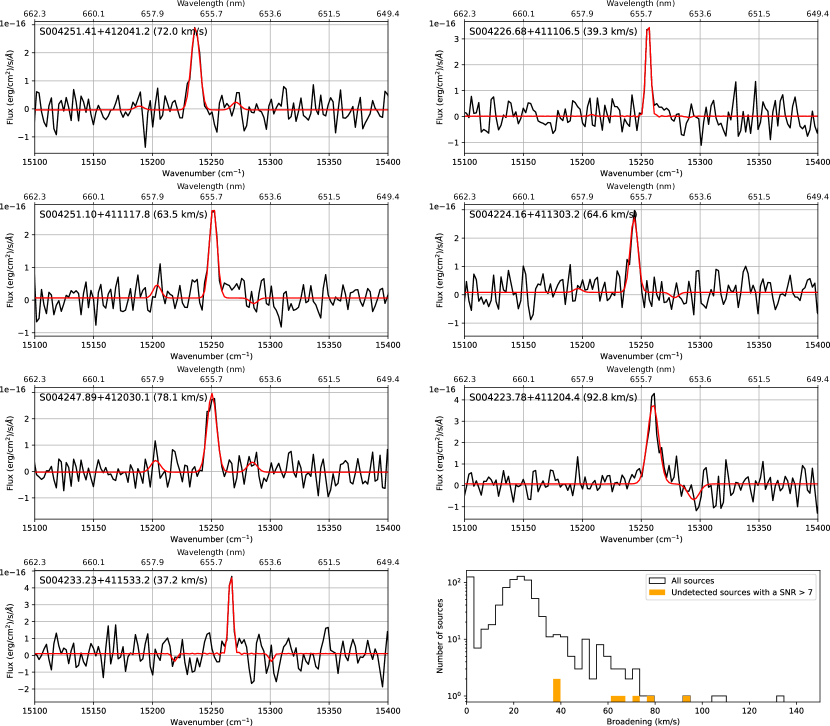
Figure 14: Spectra, cropped around the H$\alpha$ lines and the [N ii] doublet, of the seven sources having a SNR greater or equal to 7 and undetected in the LGGS ratio images (see text for details). The fit of the 3 lines is shown in solid red. The source id, as well as the width of the H$\alpha$ line are indicated above each spectrum. At the bottom-right, we show the histogram of the line broadening of all the sources (black line) and the broadening of the seven displayed sources (orange bars). Two of the three objects with a broadening larger than 100 km/s have a split profile (see section 3.3.3). The apparent bimodality of the histogram (with two peaks at 22 and 0 km s^-1) is an artefact of the fitting algorithm which can be reproduced when fitting low signal-to-noise ratio lines (see text for details).

3.3.3 Split profiles

Four sources are displaying split profiles which are shown in Figure 15. They have been added the commentary “Split” in the catalogue. The first object (S004306.42+411637.5) is clearly an expanding nebula with a velocity difference of 90.7$\pm$1.4 km s^-1 between the two components. The second object (S004243.28+411158.2) could also be seen as a single line with two satellites lines or a broadened line with some absorption (like a PCygni profile). No [S ii] lines are detected in its spectrum, and no stellar source is seen in the deep SN3 image. The three others show a broad, split H$\alpha$ line, with no evidence for forbidden lines. A relatively bright point source is visible in the deep SN3 image in all cases.

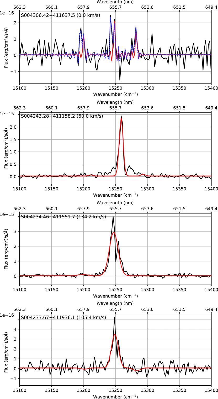
Figure 15: Spectra of sources showing split profile. The observed spectrum is displayed in black. We can clearly see the departure from the fitted model, in red. The measured broadening of the lines is reported in parenthesis. The top spectrum is clearly an expanding shell. The red-shifted and the blue-shifted components have been fitted together. The resulting fit is plotted in dotted blue. The measured expansion velocity is 90.7$\pm$1.4 km s^-1. As it was fitted with a sinc model the broadening of the lines is, by definition, 0 km s^-1.

3.3.4 Elongated PSF

A non negligible fraction of the outer portion of the field of view shows an elongated point spread function. The origin of the elongation is still unknown and could be related to an error in the model of the telescope or the optics of SITELLE (Drissen et al. in preparation). The 89 sources found in the affected region were marked with the commentary “elongated PSF”. As 90 % of the flux is concentrated in the principal lobe of the PSF the effect on the completeness is likely to be under 10–15 %. The computed flux is also likely to be underestimated by the same amount. The measured velocity suffers the same bias as the sky lines and as thus been calibrated. No velocity bias should be observed.

3.4 Comparison with the catalogue of Halliday et al. (2006)

Halliday et al. (2006) (henceforth Ha06) have measured the radial velocity of 723 planetary nebulae in M 31, 154 of which are present in the field observed with SITELLE. We have detected 148 of them (96 %) which is an excellent completeness rate considering the fact that our detection is based on the H$\alpha$ while theirs is based on the usually brighter [O iii] line.

We have plotted their velocities against ours and found that they fall very near the one-to-one line (Fig. 16). The histogram of the velocity difference with Ha06 is also shown in Fig. 16. The median difference is 1.8 km s^-1 and the standard deviation is 6.1 km s^-1. If we quadratically sum the uncertainty reported by Ha06 and ours, the median uncertainty on the velocity difference is 5.6 km s^-1. These results confirms at the same time their calibration and ours as long as both quoted uncertainties are correct. Because we could not have any precise measurement of the OH lines velocity in the center of the field of view, we have been using a model to estimate the velocity correction in the center based on the values obtained on the borders of field (see section 2.2 and Fig. 4). Any error on the model would translate into a correlation between the velocity difference and the radius with respect to the center of the image. This is not the case (see Fig. 17). We have also checked that there was no correlation with the velocity and that the difference was getting smaller at higher flux (Fig. 17). Note that Ha06 are measuring the [O iii] lines while we are providing the flux in H$\alpha$; those two properties are only partially correlated.

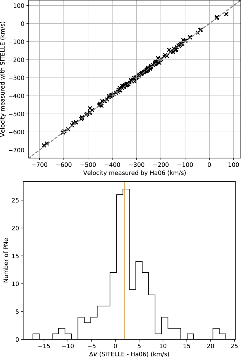
Figure 16: Top: Velocity measured with SITELLE vs. velocity measured by Ha06. The one-to-one line is shown in dotted grey. Bottom: Histogram of the velocity difference with Ha06. The median of the distribution is shown in orange.

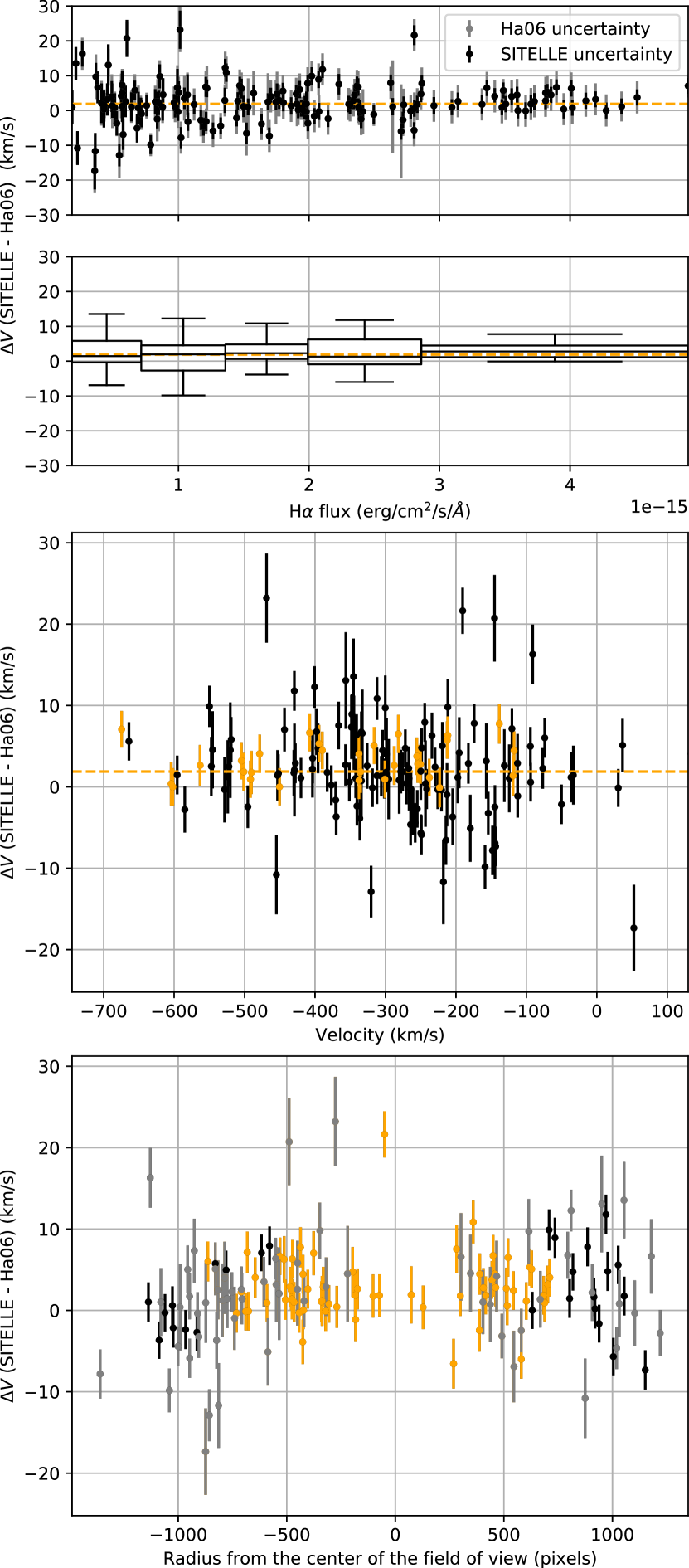
Figure 17: Top: Velocity difference with Ha06 vs. H$\alpha$ flux. The box plot represents the distribution of the difference by bins of equal number of data points. Center: Velocity difference with Ha06 vs. velocity. The 10 % most luminous sources are shown in orange Bottom: Velocity difference with Ha06 vs. radius with respect to the center of the field of view (the radius is set negative when the distance along the declination axis, i.e. the y axis, is negative). The sources in orange are situated in the region where the sky lines velocity could not be measured. Their calibration thus heavily rely on the model described in section 2.2.1.

When comparing the position of our sources with the position reported by Ha06, we find a median difference of $0.46\,\arcsec$ (Ha06 quote an absolute uncertainty of $1\,\arcsec$, with a relative uncertainty of $0.4\,\arcsec$ on their positions), with a standard deviation of $0.21\,\arcsec$, which is smaller than one SITELLE pixel and very similar to our estimate of the uncertainty (see Fig. 18).

The comparison with the catalogue of Ha06 therefore confirms the quality of our wavelength and astrometric calibration.

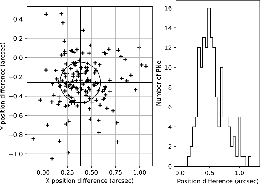
Figure 18: Left: Scatter of the position differences along the X and Y axes of the image of the sources compared with Ha06. The vertical and the horizontal black lines indicate the median of the differences in X and Y respectively. A circle represents the standard deviation. Right: Histogram of the position differences with Ha06.

3.5 Comparison with the catalogue of Merrett et al. (2006)

Merrett et al. (2006) (henceforth Me06) have measured the radial velocity of 2615 planetary nebulae in M 31, 330 of which are present in the field observed with SITELLE. We have detected 305 of them (92 %) which is a good completeness rate considering the fact that our detection is based on the H$\alpha$ while theirs is based on the usually brighter [O iii] line. The quoted uncertainty on their measurement is 17 km s^-1 with a systematic error around 5–10 km s^-1 which is much higher than the uncertainty of Ha06’s catalog. The distribution of the velocity difference with their catalogue is shown in Figure 19. This distribution’ standard deviation of 16 km s^-1 is strongly dominated by the uncertainty of their measurement and confirms their estimation. The distribution is also biased by 16 km s^-1 which is also consistent with the comparison they made with the data of Ha06 (they found a systematic difference of 17 km s^-1).

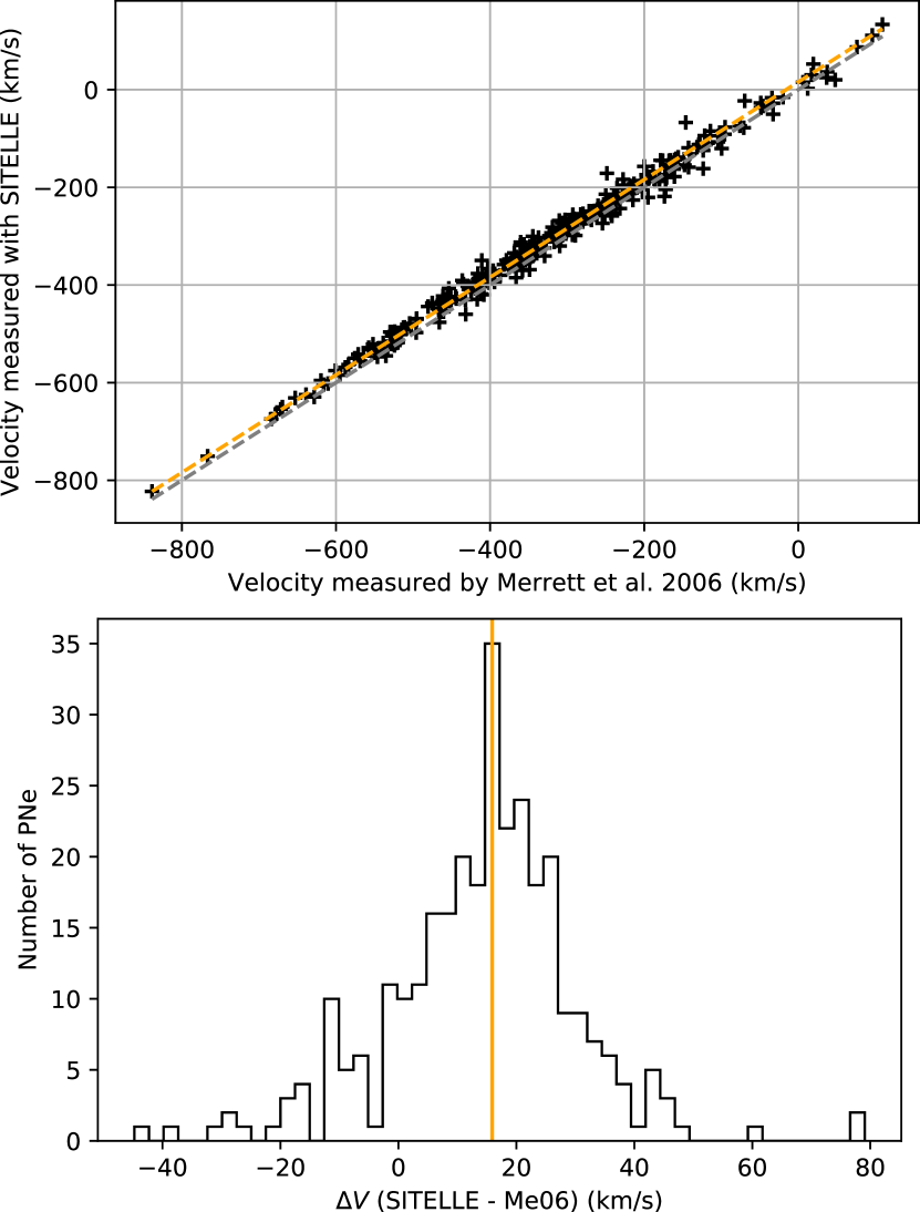
Figure 19: Top: Velocity measured with SITELLE vs. velocity measured by Me06. The one-to-one line is shown in dotted grey. The same line corrected for the median of the distribution of the velocity difference (see bottom histogram) is shown in dotted orange. Bottom: Histogram of the velocity difference with Me06. The median of the distribution is shown in orange.

We can further check the quality of our photometry by comparing the flux ratio F([O iii])/F(H$\alpha$ + [N ii]) with respect to the relative m₅₀₀₇ magnitude reported in their catalogue. Note that the [O iii]flux also comes from their value of $m_{5007}$ since Me06:

$$m_{5007}=-2.5\log\left(F(\textup{[O\,{iii}]})\right)-13.74\;.$$ (20)

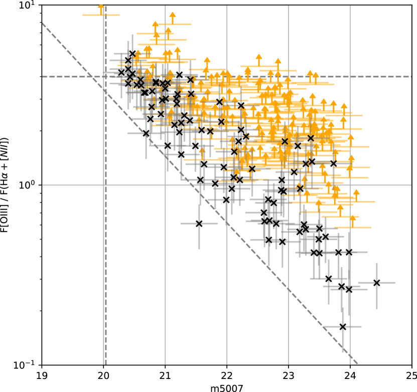
Figure 20: Flux ratio F([O iii])/F(H$\alpha$ + [N ii]) with respect to the relative m₅₀₀₇ magnitude from Me06. The sources which [N ii] line flux could only be given an upper limit are plotted in orange. The other are plotted with black crosses. The error bars are also shown. The region in this graph where all the planetary nebulae are supposed to be is defined by the 3 dotted gray lines. The vertical line corresponds to the planetary nebulae luminosity function zero-point quoted by Ciardullo et al. (2002) and the two others are defined in Herrmann et al. (2008).

We can see that most of our common sources fall in the wedge-like zone where we can find all the planetary nebulae of the Local Group Galaxies M31 and M33 (Schönberner et al., 2010). This zone is located between the lines defined by Herrmann et al. (2008):

$$\log\left(\frac{F(\text{{[O\,{iii}]}})}{F(\text{{H}$\alpha$}+\text{{[N\,{ii}]}})}\right)=-0.37M(\textup{[O\,{iii}]})-1.16\;,$$ (21)

and

$$\log\left(\frac{F(\text{{[O\,{iii}]}})}{F(\text{{H}$\alpha$}+\text{{[N\,{ii}]}})}\right)\simeq 4\;,$$ (22)

where $M(\textup{[O\,{iii}]})$ is the absolute magnitude in the [O iii]$\lambda 5007$ line which has been computed from the relation

$$M(\textup{[O\,{iii}]})=m_{5007}-A_{V}-\mu\;,$$ (23)

considering the values of the reddening $E(B-V)=0.062$ mag (Schlegel et al., 1997) and a distance $D$ to M 31 of 750 kpc (Freedman et al., 2000) which translate to an interstellar extinction $A_{V}=3.1E(B-V)=0.19$ mag and a distance modulus $\mu=5\log(D)-5=24.38$ mag. We have chosen here the same references as Ciardullo et al. (2002) to keep its value of the planetary nebulae luminosity function zero-point $M_{\star}=-4.53$ mag which is also reported in Figure 20.

3.6 Objects not listed in the catalogue

3.6.1 Novae

Between 65 and 100 novae erupt each year in M31 (Darnley et al., 2006; Chen et al., 2016; Soraisam et al., 2016), about a third of which are detected. Between January 11 (first nova detected in 2016) and August 24 (the day of our observations), seven nova candidates were detected in SITELLE’s field of view but only two of them (Nova M31 2016-08d and 05b) have been spectroscopically confirmed, both as type FeII novae. Spectra of five of our sources displayed an excessive broadening compared to all other objects (see the lower right panel of Fig. 14): all of them were indeed in the list of nova candidates. These objects are listed in Table 5 but not in the catalogue because of their transient nature; their spectra are shown in Figure 21. We therefore confirm the nova nature of three previously unconfirmed candidates (2016-03b, 03c and 03d) whereas two candidates (2016-06b and 03e) do not display obvious nova signature in our data.

Table 5: Novae visible in our data. The associated spectra are shown in Figure 21.

ID	Detection date	Atel #	Type	Coordinates	Reference
M31N 2016-03b	2016 Feb. 26.737 UT	#8785	—	0:42:19.54 +41:11:14.0	Hornoch & Kucakova (2016)
M31N 2016-03c	2016 Feb. 7.753 UT	#8787	—	0:42:49.25 +41:16:40.16	Hornoch et al. (2016)
M31N 2016-03d	2016 Mar. 17.768 UT	#8838	—	0:43:01.58 +41:14:08.7	Hornoch & Vrastil (2016)
M31N 2016-05b	2016 May 28.046 UT	#9098	Fe II	0:42:42.88 +41:15:27.1	Darnley & Williams (2016)
M31N 2016-08d	2016 Aug. 17.102 UT	#9388	Fe II	0:42:23.53 +41:17:19.8	Williams et al. (2016)

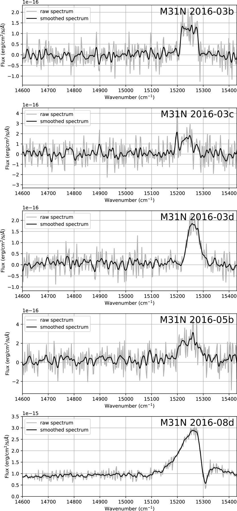
Figure 21: Novae spectra extracted from the data cube. Note that the integration region is smaller than the object size to enhance the SNR. The real flux of the nova should be considered as a lower limit and may be up to 50% higher. The background-subtracted spectrum is plotted in grey and the fit is plotted in black.

3.6.2 Supernova remnants

Three supernova remnants (SNR) were previously known in SITELLE’s field (Lee & Lee, 2014; Williams et al., 2004; Sasaki et al., 2012). These SNR are all presumably from Type Ia events since there is no signature of recent star formation in our field of view: recent studies found no H ii regions (Azimlu et al., 2011) or young clusters ($<1$ Gy) (Kang et al., 2011) and the dust seems to be only heated by the old stellar population (Viaene et al., 2014).

They clearly stand out in our cube, and we have detected one more (labeled SNR2). We have used the same criteria as Lee & Lee (2014), based on Braun & Walterbos (1993), to classify this supernova remnant: an [SII]/H$\alpha$ ratio greater than 0.4 (0.464$\pm$0.086 in our case) and the absence of a blue star. The basic characteristics of these four supernova remnants are presented in table 6. The corresponding spectra are shown in Figure 22.

Table 6: Characteristics of the observed supernova remnants.

ID	other ID	Coordinates	Radial velocity (km/s)	Broadening (km/s)
SNR1	1050b	0:42:50.50 +41:15:56.19	-320.5 $\pm$ 3.0	58.4$\pm$2.1
SNR2	—	0:42:25.07 +41:17:34.79	-429.5 $\pm$ 4.9	59.2$\pm$4.6
SNR3	#41a, r2-57c	0:42:24.68 +41:17:30.79	-101.0 $\pm$ 3.8	47.2$\pm$3.1
SNR4	#43a	0:42:25.67 +41:17:49.19	-351.5 $\pm$ 3.7	37.3$\pm$3.3
a Lee & Lee (2014).
b Stiele et al. (2011) and Sasaki et al. (2012).
c Williams et al. (2004).

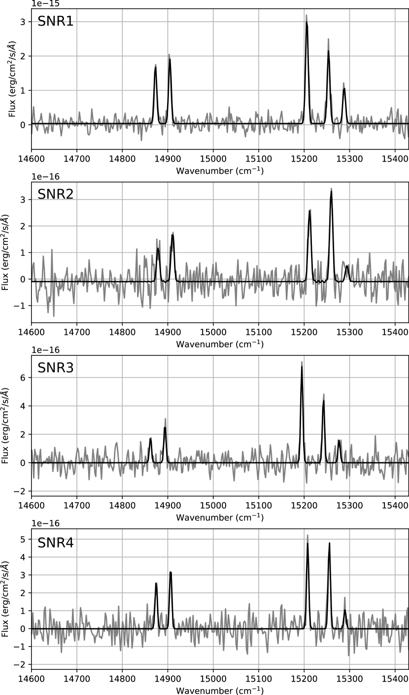
Figure 22: Integrated spectra of the supernovae remnants. The spectrum of the SNR3 has not been integrated over the whole visible region but only on its brightest knot. The background-subtracted spectrum is plotted in grey and the fit is plotted in black.

SNR1

SNR1 is clearly present in the H$\alpha$ and [S ii] images (field 5) provided by the Local Group Survey (Massey et al., 2006) and it is classified as a SNR by Sasaki et al. (2012) but it has not been selected as a supernova remnant candidate by the team, although our spectrum clearly shows strong [S ii] lines; all its lines are broader than the instrumental resolution. A detailed analysis of this object, #1050 in the catalogue of Stiele et al. (2011), in the X-ray and optical wavelengths can be found in Sasaki et al. (2012). They report an H$\alpha$ flux of 7.5 $10^{-15}$$\pm$4.4 $10^{-16}$ erg cm^-2 s^-1 and a mean [S ii] flux of 7.7 $10^{-15}$$\pm$1.5 $10^{-15}$ erg cm^-2 s^-1 which compares well with our fluxes of 6.8 $10^{-15}$$\pm$4.7 $10^{-16}$ erg cm^-2 s^-1 for H$\alpha$ and 5.8 $10^{-15}$$\pm$3.2 $10^{-16}$ erg cm^-2 s^-1 for [S ii] measured on the integrated spectrum shown in figure 22. Images of its spatially resolved emission in H$\alpha$, [N ii] and [S ii] are shown in Figure 23.

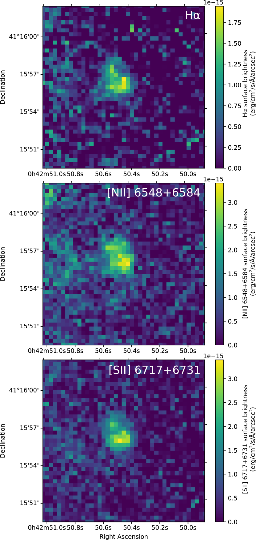
Figure 23: Flux maps in H$\alpha$, [N ii] and [S ii] of the supernova remnant SNR1. It is catalogued as the X-ray source 1050 in Stiele et al. (2011). It has been classified as a SNR and studied in details by Sasaki et al. (2012).

SNR2, SNR3 and SNR4

Three of of the four SNRs in SITELLE’s field (Lee & Lee 41 and 43, as well as our new SNR2) are within 30$\,\arcsec$ of each other (see figure 24). If SNR3 shows a velocity much different from SNR2 and SNR4, the latter have a velocity difference of only 80 km s^-1 (see Table 6), suggesting that they could be related to the same event making the remnant 60 pc wide which is a little larger than the galactic supernova remnant NGC 6960. The detection map, which shows the highest intensity in the spectrum of each pixel relatively to its neighbourhood is shown in Figure 24. A detailed study of the SNR3 (named r2-57 in their article) in the X-ray, optical and radio wavelengths can be found in Williams et al. (2004). In their Figure 3, the [S ii] emission of the SNR2 can also be seen but nothing’s found in the [O iii] image of the LGGS (Massey et al., 2006) while the SNR3 is clearly visible.

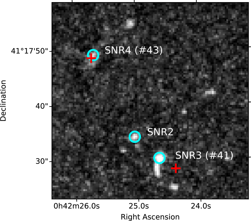
Figure 24: Small part of the detection map (see section 3.1) showing the proximity of 3 of the 4 supernovae remnants detected in the central region of M 31. Red crosses show the position of the center of the remnants reported in the catalogue of Lee & Lee (2014). Blue circles indicate the regions integrated to compute the spectra shown in figure 22. Note that we have chosen the brightest node of the remnant which has no reason to be the same as the central position reported by Lee & Lee (2014).

The H$\alpha$ surface brightness map of SNR2 and the [N ii] surface brightness map of SNR4 (Lee & Lee 43), the most extended of all four SNRs in our field ($8\,\arcsec\sim 30$ pc), are shown in Figure 25.

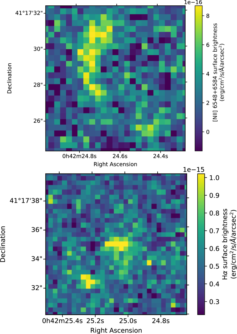
Figure 25: Top: [N ii] surface brightness map of the supernova remnant SNR3 (#41 of Lee & Lee 2014, r2-57 in Williams et al. 2004). Bottom: H$\alpha$ surface brightness map of the newly discovered supernova remnant SNR2.

4 Conclusions

We have documented and demonstrated the quality of a set of general calibration methods for SITELLE which has been applied to a spectral cube covering the center of M 31 in the H$\alpha$–[N ii]–[S ii] range (649–684 nm). Although the main target of this dataset was to study line ratios and kinematics of the diffuse gas surrounding the core of M 31 (Melchior et al., in preparation), one of the first side effects of this project is the publication of the larger and the most precise catalogue of the H$\alpha$-emitting point sources in the central region where the background flux is so high that emission-line sources are less detectable than on the outskirt. This is also a very interesting test since the detection of these sources has been made in the worst possible conditions for a Fourier transform spectrometer considering the very high continuum background of the target. Nevertheless, the number of known emission-line point-sources in this region is more than two times larger than the previously published catalogues, 5 novae spectra have been obtained as long as spatially resolved data of 4 supernovae remnants, one of them being a new discovery. Great care was taken to compare the obtained data with the best catalogues (Merrett et al., 2006; Halliday et al., 2006) and images (Massey et al., 2006) of this region which demonstrate the quality of the calibration as long as the completeness of the catalogue. A deeper analysis of this catalogue combined with the data obtained in the [O iii]–H$\beta$ range will be made in the subsequent articles. We believe that the quality of the calibration made will prove useful for all the other studies made with this data cube.

Appendix A Relation between the incident angle and the measured wavenumber

When light enters a Michelson interferometer at a null incident angle (see Figure 26), the optical path difference (OPD) $x$ is simply two times the mechanical distance $\Delta x$ between the actual position of the moving mirror and the position where both mirrors are at the same distance of the beamsplitter (known as the zero path difference position, ZPD):

$$x=2\Delta x$$ (24)

When the incident angle $\theta$ is different from 0 the OPD is known to be (see e.g. Davis et al. 2001 p. 70)

$$OPD=x\cos(\theta)$$ (25)

For the sake of clarity and for future reference we reproduce here the demonstration of this relation as given in the thesis of Grandmont (2006).

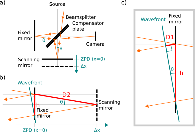
Figure 26: a) Optical path of the light at an incident angle $\theta$ in a classical Michelson interferometer. b) Superposition of the optical path followed by the light in the fixed mirror arm and the moving mirror arm. The moving mirror is at a mechanical distance $\Delta x$ from the ZPD (the position where both mirrors are at the same distance of the beamsplitter). $D2$ is the optical distance crossed by light along the moving mirror path. c) Zoomed-in portion of figure b) showing the optical distance $D1$ crossed by light along the fixed mirror path.

The OPD at any given incident angle is, by definition, the difference between the distance crossed by light in the fixed mirror arm ($D1$) and the moving mirror arm ($2\times D2$) measured on the wavefront, i.e. perpendicularly to the light direction:

$$OPD=2\times D2-D1\;.$$ (26)

A superposition of both optical paths is shown on Figure 26. From simple geometrical consideration we can deduce that $D2=\Delta x/\cos(\theta)$, $h=2\,D2\,\sin(\theta)$ and $D1=h\sin(\theta)$ from which it follows that

$$D1=2\,D2\,\sin(\theta)^{2}\;.$$ (27)

We can finally write

$$OPD=2\frac{\Delta x}{\cos(\theta)}\left(1-\sin(\theta)^{2}\right)=2\Delta x\cos(\theta)=x\cos(\theta)$$ (28)

The effect on the measured wavenumber $\sigma$ of a single emission-line of real wavenumber $\sigma_{0}$ is illustrated on Figure 27. As the OPD of the light coming with an incident angle is smaller, the interferogram of the source is sampled at shorter steps. If the centroid of the line is calculated considering the step size measured on-axis by the mirror controller the same emission-line will thus see its observed wavenumber increased by a factor $1/\cos(\theta)$ i.e.:

$$\sigma=\frac{\sigma_{0}}{\cos\theta}$$ (29)

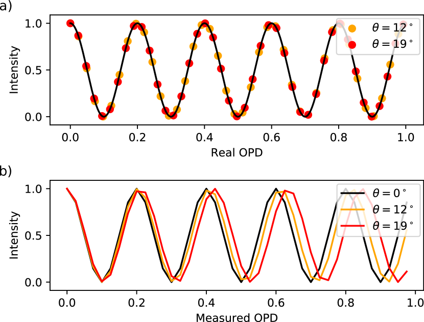
Figure 27: Effect of the incident angle $\theta$ on the sampling step-size and the measured frequency of an emission-line. a) Positions of the recorded samples of the interferogram of a monochromatic line at two incident angles 12^∘ and 19^∘ (corresponding roughly to the top and bottom pixels of the field of view). b) Recorded interferograms at three different incident angles (on-axis and at 12^∘ and 19^∘). The measured OPD of each sample, which differs from the real OPD, is the on-axis OPD i.e. the target OPD of the mirror controller. The variation of the measured wavelength of the emission line appears clearly.

Appendix B Excerpt from the catalogue

Table 7: Excerpt from the catalogue.

ID

$\alpha_{2000}$

$\delta_{2000}$

$V$a

$\epsilon_{V}$a

$\sigma$a

$\epsilon_{\sigma}$a

$F$(H$\alpha$)b

$\epsilon_{F(\text{H}\alpha)}$b

$F(\text{{[N\,{ii}]}{}}\,\lambda 6584$)b

$\epsilon_{F(\text{{[N\,{ii}]}{}}\,\lambda 6584)}$b

$F(\text{{[S\,{ii}]}{}}$)b

$\epsilon_{F(\text{{[S\,{ii}]}{}})}$b

Me06c

Ha06d

Ma06 H$\alpha$e

Ma06 [O iii]e

Comments

S004236.99+411209.3

00 42 36.99

+41 12 09.3

-0595.6

+0002.4

+0032.9

+0001.0

2.35e-15

1.23e-16

1.78e-15

1.00e-16

<4.1e-16

—

2806

P69

Sat.

Sat.

—

S004239.81+411641.5

00 42 39.81

+41 16 41.5

-0175.5

+0002.5

+0020.0

+0001.9

2.30e-15

1.64e-16

1.73e-15

1.41e-16

<6.3e-16

—

—

—

Sat.

Sat.

—

S004241.24+411909.5

00 42 41.24

+41 19 09.5

-0144.7

+0002.7

+0011.6

+0004.1

8.51e-16

7.13e-17

<1.2e-16

—

<2.1e-16

—

802

P105

Sat.

Sat.

—

S004254.20+411336.8

00 42 54.20

+41 13 36.8

-0341.0

+0002.5

+0020.6

+0001.9

1.24e-15

8.20e-17

<2.2e-16

—

<1.5e-16

—

1241

P475

Sat.

Sat.

—

S004242.16+411820.3

00 42 42.16

+41 18 20.3

+0045.4

+0004.2

+0057.4

+0003.6

2.25e-15

2.08e-16

<5.1e-16

—

<2.6e-16

—

—

—

Sat.

Sat.

—

S004229.73+411351.8

00 42 29.73

+41 13 51.8

-0504.5

+0002.3

+0022.4

+0000.8

4.26e-15

1.96e-16

1.55e-15

9.51e-17

<5.0e-16

—

1131

P98

Sat.

Sat.

—

S004254.94+411257.2

00 42 54.94

+41 12 57.2

-0438.5

+0002.3

+0023.1

+0001.0

1.80e-15

9.47e-17

1.48e-15

8.20e-17

<3.2e-16

—

—

—

Sat.

Sat.

—

S004244.51+411813.4

00 42 44.51

+41 18 13.4

-0022.9

+0002.5

+0017.1

+0002.1

1.86e-15

1.24e-16

7.56e-16

8.11e-17

<3.4e-16

—

3029

—

Sat.

Sat.

—

S004302.60+411558.3

00 43 02.60

+41 15 58.3

-0040.2

+0002.3

+0019.4

+0001.2

1.74e-15

9.89e-17

1.79e-15

1.01e-16

<4.1e-16

—

—

—

Sat.

Sat.

—

S004235.97+411410.5

00 42 35.97

+41 14 10.5

-0280.7

+0002.6

+0019.9

+0002.2

1.29e-15

1.04e-16

9.87e-16

9.10e-17

<2.7e-16

—

1205

—

Sat.

Sat.

—

S004257.87+411243.4

00 42 57.87

+41 12 43.4

-0186.2

+0002.3

+0028.1

+0000.9

2.52e-15

1.23e-16

4.86e-16

5.09e-17

<2.3e-16

—

1232

—

Sat.

Sat.

—

S004257.70+411951.0

00 42 57.70

+41 19 51.0

-0324.2

+0002.3

+0016.5

+0001.4

1.69e-15

9.28e-17

1.00e-15

6.69e-17

<2.8e-16

—

809

—

Sat.

Sat.

—

S004239.73+411839.4

00 42 39.73

+41 18 39.4

-0362.3

+0002.4

+0021.1

+0001.4

1.92e-15

1.10e-16

3.83e-16

5.66e-17

<3.2e-16

—

—

—

Sat.

Sat.

—

S004255.48+411721.1

00 42 55.48

+41 17 21.1

-0287.6

+0002.4

+0034.2

+0000.9

3.79e-15

1.97e-16

2.94e-15

1.63e-16

7.61e-16

1.33e-16

1268

P30

Sat.

Sat.

—

S004245.85+411735.4

00 42 45.85

+41 17 35.4

+0020.3

+0002.6

+0022.9

+0002.0

1.75e-15

1.36e-16

1.37e-15

1.20e-16

<6.4e-16

—

1360

—

Sat.

Sat.

—

S004242.48+411356.4

00 42 42.48

+41 13 56.4

-0413.6

+0002.7

+0029.9

+0001.7

1.90e-15

1.36e-16

1.20e-15

1.05e-16

<5.7e-16

—

1246

—

Sat.

Sat.

—

S004231.48+411614.7

00 42 31.48

+41 16 14.7

-0378.7

+0002.6

+0020.1

+0002.2

1.44e-15

1.07e-16

<3.1e-16

—

<2.3e-16

—

1162

—

Sat.

Sat.

—

S004239.57+411831.6

00 42 39.57

+41 18 31.6

-0261.0

+0002.7

+0021.7

+0002.4

1.23e-15

9.74e-17

<2.9e-16

—

<2.4e-16

—

3270

P102

Sat.

Sat.

—

S004235.29+411446.0

00 42 35.29

+41 14 46.0

-0255.4

+0002.3

+0022.3

+0000.9

4.59e-15

2.21e-16

7.73e-16

8.88e-17

<3.2e-16

—

1139

P53

Sat.

Sat.

—

S004246.10+411516.5

00 42 46.10

+41 15 16.5

-0192.7

+0002.9

+0028.3

+0002.1

2.43e-15

1.92e-16

<4.8e-16

—

<1.9e-16

—

1287

—

Sat.

Sat.

—

S004256.13+411632.5

00 42 56.13

+41 16 32.5

-0172.2

+0002.5

+0020.0

+0001.7

1.57e-15

1.10e-16

1.53e-15

1.09e-16

<3.7e-16

—

—

—

Sat.

Sat.

—

S004305.91+411846.0

00 43 05.91

+41 18 46.0

-0550.1

+0002.5

+0020.1

+0001.7

1.38e-15

8.84e-17

7.63e-16

6.43e-17

<2.8e-16

—

—

—

Sat.

Sat.

—

S004232.73+411916.9

00 42 32.73

+41 19 16.9

-0518.7

+0002.3

+0019.3

+0000.9

2.67e-15

1.25e-16

<2.2e-16

—

<2.0e-16

—

2753

—

Sat.

Sat.

—

S004229.58+411404.3

00 42 29.58

+41 14 04.3

-0275.5

+0002.4

+0022.0

+0001.2

2.34e-15

1.26e-16

9.41e-16

7.36e-17

<3.3e-16

—

1132

P50

Sat.

Sat.

—

S004251.86+411214.7

00 42 51.86

+41 12 14.7

-0555.6

+0002.3

+0025.3

+0000.7

3.53e-15

1.58e-16

<2.3e-16

—

<3.4e-16

—

1225

—

Sat.

Sat.

—

S004302.58+412028.3

00 43 02.58

+41 20 28.3

-0257.9

+0002.4

+0020.5

+0001.5

1.35e-15

7.99e-17

4.76e-16

4.77e-17

<1.9e-16

—

2755

P200

Sat.

Sat.

elongated PSF

a Velocity $V$ and broadening $\sigma$ are expressed in km s-1. The uncertainties are respectively $\epsilon_{V}$ and $\epsilon_{\sigma}$.

b Fluxes are expressed in erg cm-2 s-1. The uncertainties are represented with the letter $\epsilon$. In the case of [S ii], the reported flux is the sum of [S ii] $\lambda 6717$ and [S ii] $\lambda 6731$; in most cases only an upper limit can be given.

c Index of the cross-matched source of Merrett et al. (2006).

d Index of the cross-matched source of Halliday et al. (2006).

e Index of the cross-matched source of Massey et al. (2006) in the [O iii]/B frame or the H$\alpha$/R frame (see text for details). (T) indicates a detection ; (Sat.) indicates a saturated region.

References

- Azimlu et al. (2011) Azimlu M., Marciniak R., Barmby P., 2011, The Astronomical Journal, 142, 139
- Baril et al. (2016) Baril M. R., et al., 2016, in Evans C. J., Simard L., Takami H., eds, Proceedings of SPIE. International Society for Optics and Photonics, p. 990829
- Bohlin (2003) Bohlin R. C., 2003, The 2002 HST Calibration Workshop : Hubble after the Installation of the ACS and the NICMOS Cooling System
- Bohlin et al. (2001) Bohlin R. C., Dickinson M. E., Calzetti D., 2001, The Astronomical Journal, 122, 2118
- Braun & Walterbos (1993) Braun R., Walterbos R. A. M., 1993, Astronomy and Astrophysics Supplement Series, 98, 327
- Chen et al. (2016) Chen H.-L., Woods T. E., Yungelson L. R., Gilfanov M., Han Z., 2016, MNRAS, 458, 2916
- Ciardullo et al. (2002) Ciardullo R., Feldmeier J. J., Jacoby G. H., de Naray R. K., Laychak M. B., Durrell P. R., 2002, The Astrophysical Journal, Volume 577, Issue 1, pp. 31-50., 577, 31
- Darnley & Williams (2016) Darnley M. J., Williams S. C., 2016, The Astronomer’s Telegram, No. 9143, 9143
- Darnley et al. (2006) Darnley M. J., et al., 2006, MNRAS, 369, 257
- Davis et al. (2001) Davis S. P., Abrams M. C., Brault J. W. J. W., 2001, Fourier transform spectrometry. Academic Press, San Diego
- Drissen et al. (2010) Drissen L., Bernier A.-P., Rousseau-Nepton L., Alarie A., Robert C., Joncas G., Thibault S., Grandmont F., 2010, in McLean I. S., Ramsay S. K., Takami H., eds, Vol. 7735, SPIE Astronomical Telescopes + Instrumentation. International Society for Optics and Photonics, pp 77350B–77350B–10
- Drissen et al. (2012) Drissen L., et al., 2012, in McLean ed., Vol. 8446, SPIE - Ground-based and Airborne Instrumentation for Astronomy IV. pp 84463S–84463S–7
- Drissen et al. (2014) Drissen L., Rousseau-Nepton L., Lavoie S., Robert C., Martin T., Martin P., Mandar J., Grandmont F., 2014, Advances in Astronomy, 2014, 1
- Freedman et al. (2000) Freedman W. L., et al., 2000, The Astrophysical Journal, Volume 553, Issue 1, pp. 47-72., 553, 47
- Gaia Collaboration et al. (2016a) Gaia Collaboration G., et al., 2016a, Astronomy & Astrophysics, Volume 595, id.A2, 23 pp., 595
- Gaia Collaboration et al. (2016b) Gaia Collaboration G., et al., 2016b, eprint arXiv:1609.04153, 595
- Grandmont (2006) Grandmont F., 2006, PhD thesis, Université Laval
- Grandmont et al. (2012) Grandmont F., Drissen L., Mandar J., Thibault S., Baril M. R., 2012, in McLean I. S., Ramsay S. K., Takami H., eds, Vol. 8446, SPIE - Ground-based and Airborne Instrumentation for Astronomy IV. p. 84460U
- Halliday et al. (2006) Halliday C., et al., 2006, Monthly Notices of the Royal Astronomical Society, 369, 97
- Hanisch et al. (2001) Hanisch R. J., Farris A., Greisen E. W., Pence W. D., Schlesinger B. M., Teuben P. J., Thompson R. W., Warnock A., 2001, Astronomy and Astrophysics, 376, 359
- Herrmann et al. (2008) Herrmann K. A., Ciardullo R., Feldmeier J. J., Vinciguerra M., 2008, The Astrophysical Journal, Volume 683, Issue 2, article id. 630-643, pp. (2008)., 683
- Hook et al. (2008) Hook R. N., Simple T., Polynomial I., 2008, in Shopbell P., Britton M., Ebert R., eds, Astronomical Society of the Pacific Conference Series Vol. 347, Astronomical Data Analysis Software and Systems XIV. p. 491
- Hornoch & Kucakova (2016) Hornoch K., Kucakova H., 2016, The Astronomer’s Telegram, No. 8785, 8785
- Hornoch & Vrastil (2016) Hornoch K., Vrastil J., 2016, The Astronomer’s Telegram, No. 8838, 8838
- Hornoch et al. (2016) Hornoch K., Kucakova H., Wolf M., 2016, The Astronomer’s Telegram, No. 8787, 8787
- Kang et al. (2011) Kang Y., Rey S.-C., Bianchi L., Lee K., Kim Y., Sohn S. T., 2011, The Astrophysical Journal Supplement, Volume 199, Issue 2, article id. 37, 25 pp. (2012)., 199
- Lee & Lee (2014) Lee J. H., Lee M. G., 2014, The Astrophysical Journal, Volume 786, Issue 2, article id. 130, 18 pp. (2014)., 786
- Levenberg (1944) Levenberg K., 1944, Quarterly of Applied Mathematics, 2, 164
- Maillard et al. (2013) Maillard J. P., Drissen L., Grandmont F., Thibault S., 2013, Experimental Astronomy, 35, 527
- Marquardt (1963) Marquardt D. W., 1963, Journal of the Society for Industrial and Applied Mathematics, 11, 431
- Martin (2015) Martin T., 2015, Phd thesis, Université Laval
- Martin & Drissen (2016) Martin T., Drissen L., 2016, in Reylé C., Richard J., Cambrésy L., Deleuil M., Pécontal E., Tresse L., Vauglin I., eds, Proceedings of the annual meeting of the French Society of Astronomy & Astrophysics Lyon, June 14-17, 2016June 14-17, 2016. No. October in Proceedings of the annual meeting of the French Society of Astronomy & Astrophysics. pp 23–28
- Martin et al. (2012) Martin T., Drissen L., Joncas G., 2012, in Radziwill N. M., Chiozzi G., eds, Vol. 2, SPIE - Software and Cyberinfrastructure for Astronomy II. pp 84513K–84513K–9
- Martin et al. (2015) Martin T., Drissen L., Joncas G., 2015, Astronomical Data Analysis Software an Systems XXIV (ADASS XXIV), 495
- Martin et al. (2016) Martin T. B., Prunet S., Drissen L., 2016, Monthly Notices of the Royal Astronomical Society, 463, 4223
- Massey et al. (2006) Massey P., Olsen K. A. G., Hodge P. W., Strong S. B., Jacoby G. H., Schlingman W., Smith R. C., 2006, The Astronomical Journal, Volume 131, Issue 5, pp. 2478-2496., 131, 2478
- Merrett et al. (2006) Merrett H. R., et al., 2006, Monthly Notices of the Royal Astronomical Society, Volume 369, Issue 1, pp. 120-142., 369, 120
- Mochejska et al. (1999) Mochejska B. J., Macri L. M., Sasselov D. D., Stanek K. Z., 1999, The Astronomical Journal, Volume 120, Issue 2, pp. 810-820., 120, 810
- Moffat (1969) Moffat A. F. J., 1969, Astronomy and Astrophysics, 3
- Parzen (1962) Parzen E., 1962, The Annals of Mathematical Statistics, 33, 1065
- Rosenblatt (1956) Rosenblatt M., 1956, The Annals of Mathematical Statistics, 27, 832
- Sasaki et al. (2012) Sasaki M., Pietsch W., Haberl F., Hatzidimitriou D., Stiele H., Williams B., Kong A., Kolb U., 2012, Astronomy & Astrophysics, 544, A144
- Schlegel et al. (1997) Schlegel D. J., Finkbeiner D. P., Davis M., 1997, The Astrophysical Journal, Volume 500, Issue 2, pp. 525-553., 500, 525
- Schönberner et al. (2010) Schönberner D., Jacob R., Sandin C., Steffen M., 2010, Astronomy and Astrophysics, Volume 523, id.A86, 35 pp., 523
- Shara et al. (2016) Shara M. M., Drissen L., Martin T., Alarie A., Stephenson F. R., 2016, Monthly Notices of the Royal Astronomical Society, 465, 739
- Soraisam et al. (2016) Soraisam M. D., Gilfanov M., Wolf W. M., Bildsten L., 2016, MNRAS, 455, 668
- Stiele et al. (2011) Stiele H., Pietsch W., Haberl F., Hatzidimitriou D., Barnard R., Williams B. F., Kong A. K. H., Kolb U., 2011, Astronomy & Astrophysics, Volume 534, id.A55, 51 pp., 534
- Viaene et al. (2014) Viaene S., et al., 2014, Astronomy & Astrophysics, Volume 567, id.A71, 22 pp., 567
- Vincenty (1975) Vincenty T., 1975, Survey Review, 23, 88
- Walterbos & Braun (1992) Walterbos R. A. M., Braun R., 1992, Astronomy and Astrophysics Supplement Series (ISSN 0365-0138), vol. 92, no. 3, Feb. 1992, p. 625-682., 92, 625
- Williams et al. (2004) Williams B. F., Sjouwerman L. O., Kong A. K. H., Gelfand J. D., Garcia M. R., Murray S. S., 2004, The Astrophysical Journal, 615, 720
- Williams et al. (2016) Williams S. C., Darnley M. J., Thorstensen J. R., Klusmeyer J. A., Shafter A. W., Henze M., Hornoch K., Chinetti K., 2016, The Astronomer’s Telegram, No. 9411, 9411