Sudden Future Singularities in Quintessence and Scalar-Tensor Quintessence Models

Abstract

We demonstrate analytically and numerically the existence of geodesically complete singularities in quintessence and scalar tensor quintessence models with scalar field potential of the form $V(\phi)\sim|\phi|^{n}$ with $0<n<1$. In the case of quintessence, the singularity which occurs at $\phi=0$, involves divergence of the third time derivative of the scale factor (Generalized Sudden Future Singularity (GSFS)), and of the second derivative of the scalar field. In the case of scalar-tensor quintessence with the same potential, the singularity is stronger and involves divergence of the second derivative of the scale factor (Sudden Future Singularity (SFS)). We show that the scale factor close to the singularity is of the form $a(t)=a_{s}+b(t_{s}-t)+c(t_{s}-t)^{2}+d(t_{s}-t)^{q}$ where $a_{s},b,c,d$ are constants obtained from the dynamical equations and $t_{s}$ is the time of the singularity. In the case of quintessence we find $q=n+2$ (i.e. $2<q<3$), while for the case of scalar-tensor quintessence $q=n+1$ ($1<q<2$). We verify these analytical results numerically and extend them to the case where a perfect fluid, with a constant equation of state $w=\frac{p}{\rho}$, is present. The linear and quadratic terms in $(t_{s}-t)$ are subdominant for the diverging derivatives close to the singularity, but can play an important role in the estimation of the Hubble parameter. Using the analytically derived relations between these terms, we derive relations involving the Hubble parameter close to the singularity, which may be used as observational signatures of such singularities in this class of models. For quintessence with matter fluid, we find that close to the singularity $\dot{H}=\frac{3}{2}\Omega_{0m}(1+z_{s})^{3}-3H^{2}$. These terms should be taken into account when searching for future or past time such singularities, in cosmological data.

I Introduction

The fact that the Universe has entered a phase of accelerating expansion ($\ddot{a}>0$) Copeland et al. (2006); Frieman et al. (2008) has created new possibilities in the context of the study of exotic physics on cosmological scales. Cosmological observations of Type Ia supernova Riess et al. (1998), which were later supported by the cosmic microwave backround (CMB) Jaffe et al. (2001) and the large scale structure observations Hawking and Ellis (2011); Davis et al. (1985), are consistent with the existence of a cosmological constant ($\Lambda$CDM model) Bull et al. (2016) as the possible cause of this mysterious phenomenon. Despite the simplicity of $\Lambda$CDM and its consistency with most cosmological observations Riess et al. (1998) the required value of the cosmological constant needs to be fine-tuned in comparison with microphysical expectations. This problem has lead to the consideration of models alternative to $\Lambda$CDM . Such models include modifications of GR Nojiri and Odintsov (2006, 2003), scalar field dark energy (quintessence) Zlatev et al. (1999); Carroll (1998), physically motivated forms of fluids e.g. Chaplygin gas Bento et al. (2002); Bilic et al. (2002) etc.

Some of these dark energy models predict the existence of exotic cosmological singularities, involving divergences of the scalar spacetime curvature and/or its derivatives. These singularities can be either geodesically complete Scherrer (2005); Nesseris and Perivolaropoulos (2004); Perivolaropoulos (2005a); Lykkas and Perivolaropoulos (2016) (geodesics continue beyond the singularity and the Universe may remain in existence) or geodesically incomplete Dabrowski (2014) (geodesics do not continue beyond the singularity and the Universe ends at the classical level). They appear in various physical theories such as superstrings Antoniadis et al. (1994), scalar field quintessence with negative potentialsFelder et al. (2002), modified gravities and others Lykkas and Perivolaropoulos (2016); Barrow (2004); Fernandez-Jambrina and Lazkoz (2004). Violation of the cosmological principle (isotropy-homogeneity) by some cosmological models (e.g. modified gravity Mota and Shaw (2007), quantum effects Onemli and Woodard (2004)), has been shown to eliminate or weaken both geodesically complete and incomplete singularities Fewster and Galloway (2011); Zhang and Sasaki (2012); Bamba et al. (2012a); Nojiri et al. (2011); Bamba et al. (2012b); Barrow et al. (2011); Bouhmadi-Lopez et al. (2010); Bouhmadi-López et al. (2015); Bouhmadi-Lopez et al. (2009); Kamenshchik and Manti (2015, 2013, 2012); Dabrowski et al. (2006, 2014); Fernandez-Jambrina and Lazkoz (2009); Kamenshchik et al. (2007); Nojiri and Odintsov (2008, 2010); Sami et al. (2006); Singh and Vidotto (2011).

Geodesically incomplete singularities include the Big-Bang Penrose (1988), the Big-Rip Briscese et al. (2007); Chimento and Lazkoz (2004) where the scale factor diverges at a finite time due to infinite repulsive forces of phantom dark energy, the Little-Rip Frampton et al. (2012a) and the Pseudo-Rip Frampton et al. (2012b) singularities where the scale factor diverges at a infinite time and the Big-Crunch Felder et al. (2002); Heard and Wands (2002); Elitzur et al. (2002); Giambò et al. (2015); Perivolaropoulos (2005a); Lykkas and Perivolaropoulos (2016) where the scale factor vanishes due to the strong attractive gravity of future envolved dark energy, as e.g. in quintessence models with negative potential.

Geodesically complete singularities include SFS (Sudden Future Singularity) Barrow (2004), FSF (Finite Scale Factor) Bouhmadi-López et al. (2008), BS (Big-Separation) and the w-singularity Fernandez-Jambrina (2010). In these singularities, the cosmic scale factor remains finite but a scale factor’s derivative diverges at a finite time. The singular nature of these “singularities” amounts to the divergence of scalar quantities involving the Riemann tensor and the Ricci scalar $R=6\left(\frac{\ddot{a}}{a}+\frac{\dot{a}^{2}}{a^{2}}+\frac{k}{a^{2}}\right)$, for the FRW metric, where $a(t)$ is the cosmic scale factor Fernandez-Jambrina and Lazkoz (2006). Despite the divergence of the Ricci scalar, the geodesics are well defined at the time of the singularity. The Tipler and Krolak Tipler (1977); Krolak (1986) integrals of the Riemann tensor components along the geodesics are indicators of the strength of these singularities and remain finite in most cases. The Tipler integral Tipler (1977) is defined as

$$\int^{\tau}_{0}d\tau^{\prime}\int^{\tau}_{0}d\tau^{\prime}|R^{i}_{0j0}(\tau^{\prime\prime})|$$ (1)

while the Krolak integral Krolak (1986) is defined as

$$\int^{\tau}_{0}d\tau^{\prime}|R^{i}_{0j0}(\tau^{\prime\prime})|$$ (2)

where $\tau$ is the affine parameter along the geodesic and $R^{i}_{0j0}$ is the Riemann tensor. The components of the Riemann tensor are expressed in a frame that is parallel transported along the geodesics. If the scale factor’s first derivative is finite at the singularity, both integrals are finite (even if the second derivative of the scale factor diverges), since the Riemann tensor components involve up to second order derivatives of the scale factor. If, however, the first derivative of the finite scale factor diverges, then it is easy to see from the above integrals that only the Tipler integral is finite at the singularity, while the Krolak integral diverges. This implies an infinite impulse on the geodesics, which dissociate all bound systems at the time of the singularity Perivolaropoulos (2016); Nesseris and Perivolaropoulos (2004). The singularities that lead to the divergence of the above integrals are defined as strong singularities Rudnicki et al. (2002, 2006).

It is interesting to connect these singularities with the properties of the cosmic energy-momentum tensor. In FRW spacetime with metric

$$ds^{2}=-dt^{2}+a^{2}(t)\bigg{[}\frac{dr^{2}}{1-kr^{2}}+r^{2}(d\theta^{2}+\sin^{2}\theta d\phi^{2})\bigg{]}$$ (3)

we assume standard Einstein-Hilbert action

$$\mathcal{S}=\int\left[\frac{1}{16\pi G}R+\mathcal{L}_{(fluid)}\right]\sqrt{-g}d^{4}x$$ (4)

The Friedmann equations obtained by variation of the above action connect the density and pressure with the cosmic scale factor $a(t)$:

$$\rho(t)=\frac{3}{8\pi G}\left(\frac{\dot{a}^{2}}{a^{2}}+\frac{k}{a^{2}}\right)$$ (5)

$$p(t)=-\frac{1}{8\pi G}\left(2\frac{\ddot{a}}{a}+\frac{\dot{a}^{2}}{a^{2}}+\frac{k}{a^{2}}\right)$$ (6)

where the density and pressure are connected by the continuity equation:

$$\dot{\rho}(t)=-3\frac{\dot{a}}{a}\left[\rho(t)+p(t)\right].$$ (7)

In what follows we set $8\pi G=c=1$ and assume spatial flatness ($k=0$), in agreement with observational results and WMAP Hinshaw et al. (2013).

The divergence of the scale factor and/or its derivatives leads to divergence of scalar quantities like the Ricci scalar thus to different types of singularities or ‘cosmological milestones’ Fernandez-Jambrina and Lazkoz (2006). However geodesics do not necessarily end at these singularities and if the scale factor remains finite they are extended beyond these events Fernandez-Jambrina and Lazkoz (2004) even though a diverging impulse may lead to dissociation of all bound systems in the Universe at the time $t_{s}$ of these eventsPerivolaropoulos (2016).

Thus singularies can be classified Nojiri et al. (2005) according to the behaviour of the scale factor $a(t)$, and/or its derivatives at the time $t_{s}$ of the event or equivalently (according to eqs (5),(6)) and the energy density and pressure of the content of the universe at the time $t_{s}$. A classification of such singularities and their properties is shown in Table 1.

A particularly interesting type of singularity is the Sudden Future Singularity Barrow (2004) which involves violation of the dominant energy condition and divergence of the cosmic pressure, of the Ricci Scalar and of the second time derivative of the cosmic scale factor. The scale factor can be parametrized as

$$a(t)=\left(\frac{t}{t_{s}}\right)^{m}(a_{s}-1)+1-\left(1-\frac{t}{t_{s}}\right)^{q},$$ (8)

where $m,q,t_{s}$ are constants to be determined, $a_{s}$ is the scale factor at the time $t_{s}$ and $1<q<2$. For this range of the parameter $q$, according to eq. (5), $a,\dot{a}$ and $\rho$ remain finite at $t_{s}$. However, from eqs (6), (7) it follows that $p,\dot{\rho}$ and $\ddot{a}$ become infinite. Thus, when the first derivative of the scale factor is finite at the singularity, but the second derivative diverges (SFS singularity Barrow (2004)), the energy density is finite but the pressure diverges.

Geodesically complete singularities where the scale factor behaves like eq. (8), are obtained in various physical models such as, anti-Chaplygin gas Kamenshchik et al. (2015); Keresztes et al. (2012), loop quantum gravity Singh and Vidotto (2011), tachyonic models Gorini et al. (2004); Kamenshchik and Manti (2012, 2013, 2015), brane models Kofinas et al. (2003); Calcagni (2004); Bouhmadi-Lopez et al. (2010) etc. Such singularities however have not been studied in detail in the context of the simplest dark energy models of quintessence and scalar-tensor quintessence (see however Barrow and Graham (2015) for a qualitative analysis in the case of quintessence).

In Ref. Barrow and Graham (2015) it was shown through a qualitative analysis that a singularity of the GSFS type (see Table 1), involving a divergence of the third derivative of the scale factor, occurs generically in quintessence models with potential of the form

$$V(\phi)=A|\phi|^{n},\ \ \ \ \ A>0,$$ (9)

with $0<n<1$ and $A$ a constant parameter. This is in fact the simplest extension of $\Lambda$CDM with geodesically complete cosmic singularities and occurs at the time $t_{s}$ when the scalar field becomes zero ($\phi=0$).

Table 1: Classification and properties of cosmological singularities. The singularities discussed in the present analysis are indicated in bold.

Name	$t_{sing}$	$a(t_{s})$	$\rho(t_{s})$	$p(t_{s})$	$\dot{p}(t_{s})$	$w(t_{s})$	T	K	Geodesically
Big-Bang (BB)	0	0	$\infty$	$\infty$	$\infty$	finite	strong	strong	incomplete
Big-Rip (BR)	$t_{s}$	$\infty$	$\infty$	$\infty$	$\infty$	finite	strong	strong	incomplete
Big-Crunch (BC)	$t_{s}$	0	$\infty$	$\infty$	$\infty$	finite	strong	strong	incomplete
Little-Rip (LR)	$\infty$	$\infty$	$\infty$	$\infty$	$\infty$	finite	strong	strong	incomplete
Pseudo-Rip (PR)	$\infty$	$\infty$	finite	finite	finite	finite	weak	weak	incomplete
Sudden Future (SFS)	$\bf t_{s}$	$\bf a_{s}$	$\bf\rho_{s}$	$\bf\infty$	$\bf\infty$	finite	weak	weak	complete
Finite Sudden Future (FSF)	$t_{s}$	$a_{s}$	$\infty$	$\infty$	$\infty$	finite	weak	strong	complete
Generalized Sudden Future (GSFS)	$\bf t_{s}$	$\bf a_{s}$	$\bf\rho_{s}$	$\bf p_{s}$	$\bf\infty$	finite	weak	strong	complete
Big-Separation (BS)	$t_{s}$	$a_{s}$	0	0	$\infty$	$\infty$	weak	weak	complete
w-singularity (w)	$t_{s}$	$a_{s}$	0	0	0	$\infty$	weak	weak	complete

In the present study we extend the analysis of Barrow and Graham (2015) in the following directions:

1. We verify the existence of the GSFS both numerically and analytically, using a proper generalized expansion ansatz for the scale factor and the scalar field close to the singularity. This generalized ansatz includes linear and quadratic terms, that dominate close to the singularity and cannot be ignored when estimating the Hubble parameter and the scalar field energy density. Thus, they are important when deriving the observational signatures of such singularities.

2. We derive analytical expressions for the power (strength) of the singularity in terms of the power $n$ of the scalar field potential.

3. We extend the analysis to the case of scalar tensor quintessence with the same scalar field potential and derive both analytically and numerically the power of the singularity in terms of the power $n$ of the scalar field potential.

The structure of this paper is the following: In section II we focus on the quintessence model of eq. (9), and investigate the strength of the GSFS both analytically and numerically. In section III we extend the analysis to the case of scalar tensor quintessence and investigate the modification of the strength of the singularity both analytically (using a proper expansion ansatz) and numerically, by explicitly solving the dynamical cosmological equations. Finally, in section IV we summarise our results and discuss possible extensions of the present analysis.

II Sudden Future Singularities in Quintessence Models

II.1 Evolution without perfect fluid

Setting $8\pi G=1$, the most general action, involving gravity, nonminimally coupled with a scalar field $\phi$, and a perfect fluid is

In the special case where $F(\phi)=1$ and in the absence of a perfect fluid, the action (10) reduces to the simple case of quintessece models without a perfect fluid

$$\mathcal{S}=\int\left[\frac{1}{2}R+\frac{1}{2}g^{\mu\nu}\phi_{;\mu}\phi_{;\nu}-V(\phi)\right]\sqrt{-g}d^{4}x$$ (11)

The energy density and pressure of the scalar field $\phi$, may be written as

$\rho_{\phi}=\frac{1}{2}\dot{\phi}^{2}+V(\phi)$   and   $p_{\phi}=\frac{1}{2}\dot{\phi}^{2}-V(\phi)$.

Variation of the action (11) assuming a power law potential (9) leads to the dynamical equations

$$3H^{2}=\frac{1}{2}\dot{\phi}^{2}+V(\phi)$$ (12)

$$\ddot{\phi}=-3H\dot{\phi}-An|\phi|^{n-1}\Theta(\phi)$$ (13)

$$2\dot{H}=-\dot{\phi}^{2},$$ (14)

where $H=\frac{\dot{a}}{a}$ is the Hubble parameter, $0<n<1$ and

$$\Theta(\phi)=\begin{cases}1,&\phi>0\\ -1,&\phi<0\end{cases}$$ (15)

. This class of quintessence models has been studied extensively focusing mostly on the cosmological effects and the dark energy properties that emerge due to the expected oscillations of the scalar field around the minimum of its potential Perivolaropoulos and Sourdis (2002); Perivolaropoulos (2003); Johnson and Kamionkowski (2008); Lima et al. (2014); Dutta and Scherrer (2008). In the present analysis we focus instead on the properties of the cosmological singularity that is induced as the scalar field vanishes periodically during its oscillations. For simplicity, we consider only the first time $t_{s}$ when the scalar field vanishes during its dynamical oscillations.

The dynamical evolution of the scalar field due to the potential shown in Fig. 1 may be qualitatively described as follows Barrow and Graham (2015):

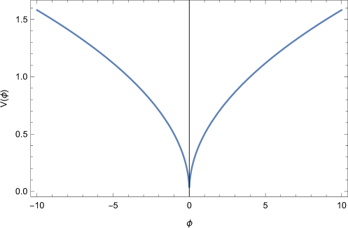
Figure 1: Exponential scalar field potential $V(\phi)=A|\phi|^{n}$

From eqs (12), (14), it follows that when $t\to t_{s}$ ($\phi\to 0$) $H,\dot{H}$ remain finite and so does $\dot{\phi}$. But in eq. (13) there is a divergence of the term $\phi^{n-1}$ for $0<n<1$ and thus $\ddot{\phi}\to\infty$ as $\phi\to 0$. $\ddot{H}$ also diverges at this point due to the divergence of $\ddot{\phi}$, as follows by differentiating eq. (14). This implies that the third derivative of the scale factor diverges, and a GSFS occurs at this point (i.e. $a_{s},\rho_{s},p_{s}$ remain finite but $\dot{p}\to\infty)$. Thus, the constraints on the power exponents $q,r$ of the diverging terms in the expansion of the scale factor ($\sim(t_{s}-t)^{q}$ ) and of the scalar field ($\sim(t_{s}-t)^{r}$ ) are $2<q<3$ and $1<r<2$ respectively (see eqs (16), (17) below).

In what follows we extend the above qualitative analysis to a quantitative level. In particular, we use a new ansatz for the scale factor and the scalar field, containing linear and quadratic terms of $(t_{s}-t)$. These terms play an important role since they dominate in the first and second derivative of the scale factor as the singularity is approached.

Thus, the new ansatz for the scale factor which generalizes (8), by introducing linear and quadratic terms in $(t_{s}-t)$ is of the form

$$a(t)=a_{s}+b(t_{s}-t)+c(t_{s}-t)^{2}+d(t_{s}-t)^{q},$$ (16)

where $b,c,d$ are real constants to be determined, and $2<q<3$ so that $\dddot{a}$ diverges at the GSFS.

The corresponding expansion of the scalar field $\phi(t)$ close to singularity is of the form

$$\phi(t)=f(t_{s}-t)+h(t_{s}-t)^{r}$$ (17)

where $f,h,$ are real constants to be determined, and $1<r<2$ so that $\ddot{\phi}$ diverges at the singularity.

Substituting eqs (16), (17) in eq. (13), we get the equation of the dominant terms

$$\mathcal{A}_{1}(t_{s}-t)^{r-2}=\mathcal{A}_{2}(t_{s}-t)^{n-1}$$ (18)

where the $\mathcal{A}_{1},\mathcal{A}_{2}$, denote constants, which may be expressed in terms of $f,h$ and the constant $A$ (see Appendix). Clearly, both the left and right-hand side of eq. (18) diverge at the singularity for $1<r<2$ and $0<n<1$. Equating the power laws of divergent terms we obtain

$$r=n+1$$ (19)

Similarly, differentiation of eq. (14) with respect to $t$ gives $2\ddot{H}=-2\dot{\phi}\ddot{\phi}$, from which we obtain an equation for the dominant terms using eqs (16), (17)

$$\mathcal{A^{\prime}}_{1}(t_{s}-t)^{q-3}=\mathcal{A^{\prime}}_{1}(t_{s}-t)^{r-2}$$ (20)

where the $\mathcal{A^{\prime}}_{1},\mathcal{A^{\prime}}_{2}$ are constants, which may be expressed in terms of $d,f,h$ (see Appendix). The left and the right-hand side of eq. (20) diverge, and therefore, equating the power laws of diverging terms we obtain

$$q=r+1.$$ (21)

Thus, using (19) and (21) we find the exponent $q$ in terms of $n$ as

$$q=n+2.$$ (22)

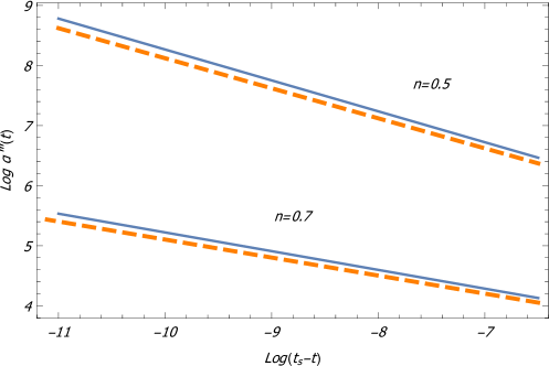
Figure 2: Numerical verification of the $q$-exponent for $n=0.5$ and $n=0.7$. The orange dashed line, denotes the analytical, while the blue line denotes the numerical solution. As expected the slopes for each n are identical.

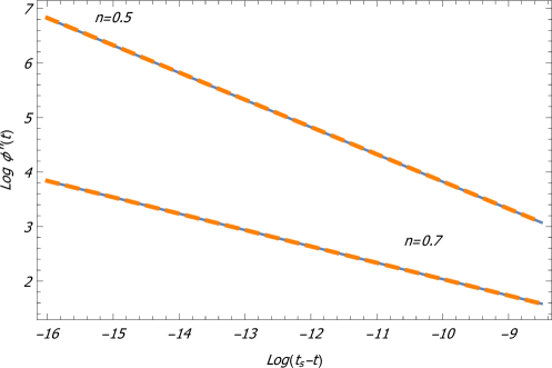
Figure 3: Same as Fig. 2 for the $r$-exponent.

Eqs (19), (22), are consistent with the qualitatively expected range of $r,q$, for $0<n<1$.

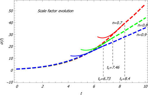
Figure 4: Plot of numerical (dashed) and analytical (line) time evolution of the scale factor, for $n=0.7,0.8,0.9$. The two solutions for each $n$ are consistent close to each singularity.

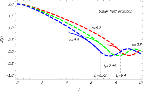
Figure 5: Numerical (dashed line) and analytical (continuous line) time evolution of the scalar field, for $n=0.7,0.8,0.9$. The two solutions for each $n$ are consistent close to each singularity.

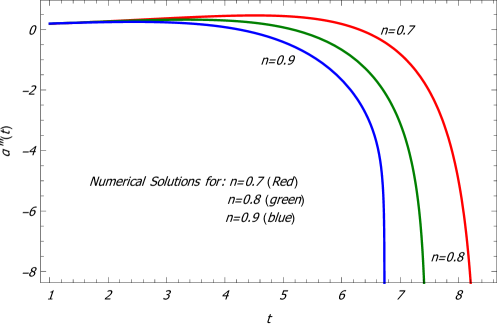
Figure 6: Numerical solutions of the third time derivative of the scale factor for $n=0.7,0.8,0.9$. Notice the divergence at the time of the singularity when the scalar field vanishes ($t_{s}=8.4$ for $n=0.7$, $t_{s}=7.46$ for $n=0.8$, $t_{s}=6.73$ for $n=0.9$).

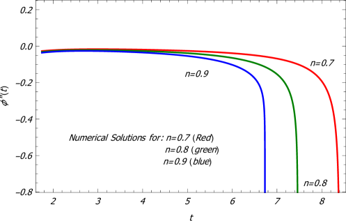
Figure 7: Numerical solutions of the second time derivative of the scalar field for $n=0.7,0.8,0.9$. Notice the divergence at the time of the singularity when the scalar field vanishes ($t_{s}=8.4$ for $n=0.7$, $t_{s}=7.46$ for $n=0.8$, $t_{s}=6.73$ for $n=0.9$).

Substituting the expressions (16), (17), (9) for $a(t),\phi(t)$ and $V(\phi)$ in the dynamical eqs. (12) and (14), it is straightforward to calculate the relations between the coefficients $c,d,f,h$. The form of the relations between the evaluated expansion coefficients, is shown in the Appendix, and has been verified by numerical solution of the dynamical equations.

The additional linear and quadratic terms in $(t_{s}-t)$, in the expression of the scale factor (16), play an important role in the estimation of the Hubble parameter and its derivative as the singularity is aproached.

The relations between these coefficients can lead to relations between the Hubble parameter and its derivative close to the singularity, which in turn correspond to observational predictions that may be used to identify the presence of these singularities in angular diameter of luminosity distance data. For example, the coeficients $b$ and $c$ are related as (see Appendix eq. (58)),

$$c=-\frac{b^{2}}{a_{s}}.$$ (23)

Using this relation, it is easy to show that

$$\dot{H}=-3H^{2}$$ (24)

(see proof in Appendix). This result constitutes an observationally testable prediction of this class of models, which can be used to search for such singularities in our past light cone.

II.2 Numerical analysis

It is straightforward to verify numerically the derived power law dependence of the scale factor and scalar field as the singularity is approached. We thus solve the rescaled, with the present day Hubble parameter $H_{0}$ (setting $H=\bar{H}H_{0}$, $t=\bar{t}/H_{0}$, $V=\bar{V}H^{2}_{0}$ ), coupled system of the cosmological dynamical equations for the scale factor and for the scalar field (13) and (14). We assume initial conditions at early times ($t\ll t_{0}$) when the scalar field is assumed frozen at $\phi(t_{i})=\phi_{i}$ and $\dot{\phi}(t_{i})=0$ due to cosmic friction Caldwell and Linder (2005); Scherrer and Sen (2008). At that time the initial conditions for the scale factor are well approximated by

$$a(t_{i})=\exp\left[\sqrt{\frac{V(\phi_{i})}{3}}t_{i}\right],$$ (25)

$$\dot{a}(t_{i}))=\sqrt{\frac{V(\phi_{i})}{3}}\left[\exp\sqrt{\frac{V(\phi_{i})}{3}}t_{i}\right]$$ (26)

Taking the logarithm of the numerical solution corresponding to the third derivative of the scale factor (16) and to the second derivative of the scalar field (17), we obtain Fig.2 and Fig.3, which show these logarithms as functions of $t_{s}-t$ close to the singularity (continous lines). On these lines we superpose the corresponding analytic expansions (eqs (16) and (17), dashed lines) which, close to the singularity, may be written as

$$\log[|\dddot{a}|]=\log[|d|q(q-1)(q-2)]+(q-3)\log[(t_{s}-t)]$$ (27)

and

$$\log[|\ddot{\phi}|]=\log[|h|r(r-1)]+(r-2)\log[(t_{s}-t)].$$ (28)

In the plots of eqs (27), (28) (dashed lines) we have used the predicted values of the exponents (eqs (19) and (22)) and the analytically predicted values for the coeficients $d$ and $h$ shown in the Appendix. We underline the good agreement in the slopes of the analytically predicted curves and the corresponding numerical results, which confirm the validity of the power law ansatz (16), (17), and the values of the corresponding exponents (19), (22)).

We have also verified this agreement by obtaining the best fit slopes of the numerical solutions of Fig.2, Fig.3 deriving the numerically predicted values of the exponents $q$ and $r$. These numerical best fit values, along with the corresponding analytical predictions, are shown in Table 2 for $n=0.5$ and $n=0.7$, indicating good agreement between the analytical and numerical values of the exponents.

In Fig.4, Fig.5 we show the time evolution (numerical and analytical) of the scale factor and the scalar field respectively. The two curves, for each $n$, are consistent close to each singularity. In Fig.6 and Fig.7 we demonstrate numerically the divergence of the third derivative of the scale factor and of the second derivative of the scalar field. The divergence occurs at the time of the singularity when the scalar field vanishes i.e. $\phi=0$.

	Numerical		Analytical
$n$	$r$	$q$	$r=n+1$	$q=n+2$
$0.5$	$1.5\pm 0.0003$	$2.51\pm 0.0007$	$1.5$	$2.5$
$0.7$	$1.7\pm 0.002$	$2.71\pm 0.004$	$1.7$	$2.7$

Table 2: Numerical and analytical values of the power exponents $r,q$. Clearly, there is consistency between numerical results and analytical expectations.

II.3 Evolution with a perfect fluid

In the presence of a perfect fluid, the action of the theory is obtained from the generalized action (10) with $F(\phi)=1$ as

$$\mathcal{S}=\int\left[\frac{1}{2}R+\frac{1}{2}g^{\mu\nu}\phi_{;\mu}\phi_{;\nu}-V(\phi)+\mathcal{L}_{(fluid)}\right]\sqrt{-g}d^{4}x.$$ (29)

The corresponding dynamical equations are

$$3H^{2}=\frac{3\Omega_{0,m}}{a^{3}}+\frac{1}{2}\dot{\phi}^{2}+V(\phi)$$ (30)

$$\ddot{\phi}=-3H\dot{\phi}-An|\phi|^{n-1}\Theta(\phi)$$ (31)

$$2\dot{H}=-\frac{3\Omega_{0,m}}{a^{3}}-\dot{\phi}^{2}$$ (32)

with $\rho_{m}=\frac{\rho_{0m}}{a^{3}}=\frac{3\Omega_{0,m}}{a^{3}}$ and $\Omega_{0,m}=0.3$. The scale factor (16), in the presence of a perfect fluid is now assumed to be of the form

$$a(t)=1+(a_{s}-1)\left(\frac{t}{t_{s}}\right)^{m}+b(t_{s}-t)+c(t_{s}-t)^{2}+d(t_{s}-t)^{q}$$ (33)

where $m=\frac{2}{3(1+w)}$ and $w$ the state parameter. As in the case of the previous section, from the dynamical equations (30), (32), $H,\dot{H},\dot{\phi}$ still remain finite. Also in eq. (31) there is a divergence of the term $\phi^{n-1}$ for $0<n<1$ and $\ddot{\phi}\to\infty$ as $\phi\to 0$. The third derivative of the scale factor $\dddot{a}$ also diverges due to the divergence of $\ddot{H}$ (differentiation of eq. (14)). Thus, the constraints for $q,r$ are the same as in the absence of the fluid (section II.1), i.e. $2<q<3$ and $1<r<2$ respectively.

Following the steps of section II.1, we rediscover the same values for the exponents i.e. eqs (19) and (22) which imply similar behaviour close to the singularity.

The relations among the expansion coefficients $c,d,f,h$, are shown in the Appendix, and have been verified by numerical solution of the dynamical equations, as in the absence of the fluid (see Appendix). For $\rho_{0m}=0$ all coefficients reduce to those of the no fluid case.

An interesting result arises from the derivation of the relation between the coefficients $b,c$. The relation between $b,c$ in the presence of a fluid is of the form (see Appendix eq. (66)),

$$c=\frac{\rho_{0,m}}{4a^{2}_{s}}-\frac{1}{2}(a_{s}-1)m(m-1)-\frac{[(a_{s}-1)m-b]^{2}}{a_{s}},$$ (34)

Thus, close to the singularity we obtain

$$\dot{H}=\frac{3}{2}\Omega_{0,m}(1+z_{s})^{3}-3H^{2}$$ (35)

where $z_{s}$ is the redshift at the time of the singularity. Clearly eq. (35) reduces to eq. (24) for $\rho_{0,m}=0$ (see proof in Appendix). This result may be used as observational signature of such singularities in this class of models.

III Sudden Future Singularities in Scalar-Tensor Quintessence Models

III.1 Evolution without a perfect fluid

We now consider now scalar-tensor quintessence models without the presence of a perfect fluid. The action of the theory is the generalized action (10), where $\mathcal{L}_{(fluid)}$ is ignored. Therefore, it has the form

$$\mathcal{S}=\int\left[\frac{1}{2}F(\phi)R+\frac{1}{2}g^{\mu\nu}\phi_{;\mu}\phi_{;\nu}-V(\phi)\right]\sqrt{-g}d^{4}x$$ (36)

We assume a nonminimal coupling linear in the scalar field $F(\phi)=1-\lambda\phi$ even though our results about the type of the singularity in this class of models is unaffected by the particular choice of the nonminimal coupling. The dynamical equations are of the form

$$3FH^{2}=\frac{\dot{\phi}^{2}}{2}+V-3H\dot{F}$$ (37)

$$\ddot{\phi}+3H\dot{\phi}-3F_{\phi}\bigg{(}\frac{\ddot{a}}{a}+H^{2}\bigg{)}+An|\phi|^{(n-1)}\Theta(\phi)=0$$ (38)

$$-2F\bigg{(}\frac{\ddot{a}}{a}-H^{2}\bigg{)}=\dot{\phi}^{2}+\ddot{F}-H\dot{F},$$ (39)

where $F_{\phi}=\frac{d}{d\phi}F$. From eq. (37), it is clear that $H,\dot{\phi},F,\dot{F}$ all remain finite when $\phi\to 0$ ($t\to t_{s}$). However, in eq. (38) there is a divergence of the term $V_{\phi}$ for $0<n<1$ and $\ddot{\phi}\to\infty$ as $\phi\to 0$. This means that $\ddot{F}\to\infty$ because of the generation of the second derivative of $\phi$ that leads to a divergence of $\ddot{a}$ in eq. (39). The effective dark energy density and pressure take the form Capozziello et al. (2007); Lykkas and Perivolaropoulos (2016)

$$\rho_{DE}=\frac{\dot{\phi}^{2}}{2}+V-3FH^{2}-3H\dot{F}$$ (40)

$$p_{DE}=\frac{\dot{\phi}^{2}}{2}-V-(2\dot{H}-3H^{2})F+\ddot{F}+2H\dot{F}.$$ (41)

Thus $\rho_{DE}$ remains finite in eq. (40), while $p_{DE}\to\pm\infty$ in eq. (41). Clearly, an SFS singularity (Table 1, see also Dabrowski et al. (2007)) is expected to occur in scalar-tensor quintessence models, as opposed to the GSFS singularity in the corresponding quintessence models. This result will be verified quantitatively in what follows.

Using the ansatz (16), (17) in the dynamical eq. (39) we find that the dominant terms close to the singularity are

$$\mathcal{B}_{1}(t_{s}-t)^{q-2}=\mathcal{B}_{2}(t_{s}-t)^{r-2}$$ (42)

where the $\mathcal{B}_{1},\mathcal{B}_{2}$ are constants, which depend on the coefficient $d,h$ and the $\lambda$ constant, and are shown in the Appendix. It immediately follows from eq. (42) that

$$q=r$$ (43)

Similarly, substituting the ansatz (16), (17) in eq. (38) we find that the dominant terms close to the singularity obey the equation

$$\mathcal{B^{\prime}}_{1}(t_{s}-t)^{r-2}=\mathcal{B^{\prime}}_{2}(t_{s}-t)^{n-1}$$ (44)

where the $\mathcal{B^{\prime}}_{1},\mathcal{B^{\prime}}_{2}$ are constants, which depend on the coefficient $f$ and the constants $A,\lambda$ as shown in the Appendix. Equating the exponents of the divergent terms we find

$$r=n+1,$$ (45)

which leads to

$$q=n+1.$$ (46)

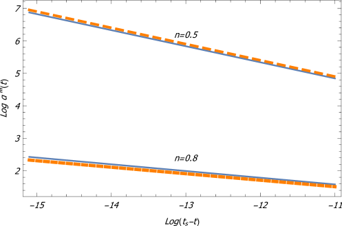
Figure 8: Numerical verification of the $q$-exponent for $n=0.5$ and $n=0.8$. The orange dashed line, denotes the analytical, while the blue line denotes the numerical solution. As expected the slopes for each n are identical, while the small difference is due to the coefficients.

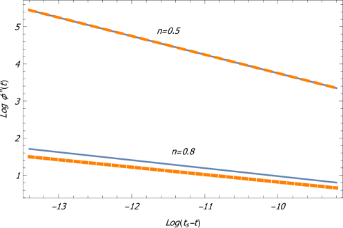
Figure 9: Numerical verification of the $r$-exponent for $n=0.5$ and $n=0.8$. The orange dashed line, denotes the analytical, while the blue line denotes the numerical solution. As expected the slopes for each n are identical, while the small difference is due to the coefficients.

The results (45) and (46) are consistent with the above qualitative discussion for the expected strength of the singularity. Thus in the case of the scalar-tensor theory we have a stronger singularity at $t_{s}$, compared to the singularity that occurs in quintessence models. This is a general result, valid not only for the coupling constant of the form $F=1-\lambda\phi$ but also for other forms of $F(\phi)$ (e.g. $F\sim\phi^{r}$), because the second derivative of $F$ with respect to time, in the dynamical equations, will always generate a second derivative of $\phi$ with divergence, leading to a divergence of $\ddot{a}$.

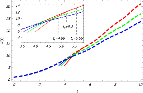
Figure 10: Plot of numerical (dashed) and analytical (line) time evolution of the scale factor, for $n=0.7$ (red), $0.8$ (green), and $0.9$ (blue). The two solutions for each $n$ are consistent close to each singularity.

Figure 11: Plot of numerical (dashed) and analytical (line) time evolution of the scalar field, for for $n=0.7$ (red), $0.8$ (green), and $0.9$ (blue). The two solutions for each $n$ are consistent close to each singularity.

Figure 12: Numerical solutions of the second time derivative of the scale factor for $n=0.7,0.8,0.9$. Notice the divergence at the time of the singularity when the scalar field vanishes ($t_{s}=5.56$ for $n=0.7$, $t_{s}=5.2$ for $n=0.8$, $t_{s}=4.88$ for $n=0.9$).

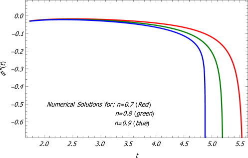
Figure 13: Numerical solutions of the second time derivative of the scalar field for $n=0.7,0.8,0.9$. Notice the divergence at the time of the singularity when the scalar field vanishes ($t_{s}=5.56$ for $n=0.7$, $t_{s}=5.2$ for $n=0.8$, $t_{s}=4.88$ for $n=0.9$).

Using eqs (37), (42), (43), (44) and (45), we calculate relations among the coefficients $c,d,f,h$. The form of these relations, is shown in the Appendix, and has been verified by numerical solution of the dynamical equations. Notice that all coefficients, except $d$, reduce to those of section II.1 for $\lambda=0$.

III.2 Numerical analysis

We now solve the rescaled coupled system of the cosmological dynamical equations for the scale factor and for the scalar field (38) and (39), using the present day Hubble parameter $H_{0}$ (setting $H=\bar{H}H_{0}$, $t=\bar{t}/H_{0}$, $V=\bar{V}H^{2}_{0}$). We assume initial conditions at early times ($t\ll t_{0}$) when the scalar field is assumed frozen at $\phi(t_{i})=\phi_{i}$ and $\dot{\phi}(t_{i})=0$ due to cosmic friction in the context of thawing Caldwell and Linder (2005); Scherrer and Sen (2008) scalar-tensor quintessence Perivolaropoulos (2005b); Nesseris and Perivolaropoulos (2007a, b). At that time the initial conditions for the scale factor are

$$a(t_{i})=\exp\left[\sqrt{\frac{V(\phi_{i})}{3F_{i}}}t_{i}\right],$$ (47)

$$\dot{a}(t_{i}))=\exp\left[\sqrt{\frac{V(\phi_{i})}{3F_{i}}}t_{i}\right]\sqrt{\frac{V(\phi_{i})}{3F_{i}}},$$ (48)

where $F_{i}=1-\lambda\phi_{i}$.

Taking the logarithm of the second derivative of the scale factor (16) and of the scalar field (17), we obtain

$$\log[|\ddot{a}|]=\log[|d|q(q-1)]+(q-2)\log[(t_{s}-t)]$$ (49)

and

$$\log[|\ddot{\phi}|]=\log[|h|r(r-1)]+(r-2)\log[(t_{s}-t)]$$ (50)

The numerical verification of the validity of eqs (45), (46) has been performed similarly to the case of minimally coupled quintessence. In Fig.8 and Fig.9 we show the analytical and numerical solutions, for the logarithm of the diverging terms of the scale factor and the scalar field respectively, as $t\to t_{s}$ from below. The $\log$-plots of the diverging terms of $\ddot{a}$ and $\ddot{\phi}$ are straight lines, indicating a power law behaviour with best fit slopes as shown in Table 3, in good agreement with the analytical expansion expectations (eqs (45), (46). In Figs.10, 11 we show the time evolution (numerical and analytical) of the scale factor and the scalar field respectively. The two curves, for each $n$, are consistent close to each singularity. In Figs.12, 13 we demonstrate numerically the divergence of the second derivarive of the scale factor and of the scalar field. As expected, the divergence occurs at the time of the singularity when the scalar field vanishes.

	Numerical		Analytical
$n$	$r$	$q$	$r=n+1$	$q=n+1$
$0.5$	$1.5\pm 0.0003$	$1.49\pm 0.0002$	$1.5$	$1.5$
$0.8$	$1.8\pm 0.03$	$1.8\pm 0.006$	$1.8$	$1.8$

Table 3: Numerical and analytical values of the power-laws $r,q$. Clearly, there is consistency between numerical results and analytical expectations.

Using eqs (49), (50), it is straightforward to obtain numerically the values of the parameters $h$ of the scalar field, as well as $d$ of the scale factor, and compare with their analytically obtained values shown in the Appendix.

The quadratic term of $(t_{s}-t)$, in the expression of the scale factor (16), is now subdominant as the second derivarive of the scale factor diverges. The only additional term of $(t_{s}-t)$ that can play an important role in the estimation of the Hubble parameter, is the linear term. Clearly, for the first derivative of (16), as $t\to t_{s}$ from below, the linear term dominates over all other terms, while the quadratic term is subdominant in the second derivative in the divergence of the $q$-term. Thus, in the case of the scalar-tensor quintessence models $H$ remain finite and dominated by the term $b(t_{s}-t)$, while $\dot{H}\to\infty$ as $t\to t_{s}$.

III.3 Evolution with a perfect fluid

In the presence of a perfect fluid, the action is now the generalized action (10). The scale factor and the scalar field are of the form (33) and (17) respectively. The dynamical equations in the presence of a relativistic fluid become

$$3FH^{2}=\frac{3\Omega_{0,m}}{a^{3}}+\frac{\dot{\phi}^{2}}{2}+V-3H\dot{F}$$ (51)

$$\ddot{\phi}+3H\dot{\phi}-3F_{\phi}\bigg{(}\frac{\ddot{a}}{a}+H^{2}\bigg{)}+V_{\phi}=0$$ (52)

$$-2F\bigg{(}\frac{\ddot{a}}{a}-H^{2}\bigg{)}=\frac{3\Omega_{0,m}}{a^{3}}+\dot{\phi}^{2}+\ddot{F}-H\dot{F}$$ (53)

The constraints for $r,q$ as $t\to t_{s}$ from below, are the same as in the absence of the fluid i.e. $1<r<2$ and $1<q<2$, and following the steps of the section III.1 we obtain

$$q=r,$$ (54)

$$r=n+1,$$ (55)

and according to eq. (54)

$$q=n+1.$$ (56)

i.e. eqs (43), (45) and (46) respectively. Finally, the form of the evaluated expansion coefficients $c,d,f,h$ is shown in the Appendix, and has been verified by numerical solution of the dynamical equations (see Appendix). As expected, for $\rho_{0m}=0$, all coefficients reduce to the ones of the no fluid case.

IV Conclusion-Discussion

We have derived analytically and numerically the cosmological solution close to a future-time singularity for both quintessence and scalar-tensor quintessence models. For quintessence, we have shown that there is a divergence of $\dddot{a}$ and a GSFS singularity occurs ($a_{s},\rho_{s},p_{s}$ remain finite but $\dot{p}\to\infty)$ , while in the case of scalar-tensor quintessence models there is a divergence of $\ddot{a}$ and an SFS singularity occurs ($a_{s},\rho_{s}$ remain finite but $p_{s}\to\infty$, $\dot{p}\to\infty)$. Importing a perfect fluid in the dynamical equations, in both cases, we have shown that this result is still valid in our cosmological solution.

These are the simplest non-exotic physical models where GSFS and SFS singularities naturally arise. In the case of scalar-tensor quintessence models, there is a divergence of the scalar curvature $R=6\left(\frac{\ddot{a}}{a}+\frac{\dot{a}^{2}}{a^{2}}\right)\to\infty$ because of the divergence of the second derivative of the scale factor. Thus, a stronger singularity occurs in this class of models. Such divergence of the scalar curvature is not present in the simple quintessence case.

We have also shown the important role of the additional linear and quadratic terms of $t_{s}-t$ in the form of the scale factor as $t\to t_{s}$. However, in the scalar-tensor case the quadratic term becomes subdominant close to the singularity.

We have derived explicitly the relations between the coefficients of the linear, quadratic and diverging terms of the scale factor and the scalar field. We have shown that all coefficients of the fluid case (quintessence and scalar-tensor quintessence), reduce to those of the no fluid case for $\rho_{0m}=0$, and all coefficients (except coefficient $d$) of the scalar-tensor models reduce to those of the simple quintessence, in the special case $\lambda=0$ i.e. $F=1$. Moreover, for quintessence models, we derived relations of the Hubble parameter, $\dot{H}=-3H^{2}$ (for the no fluid case) and $\dot{H}=\frac{3}{2}\Omega_{0,m}(1+z_{s})^{3}-3H^{2}$ (for the fluid case), close to the singularity. These relations may be used as observational signatures of such singularities in this class of models.

Interesting extensions of the present analysis include the study of the strength of these singularities in other modified gravity models e.g. string-inspired gravity, Gauss-Bonnet gravity etc Nojiri and Odintsov (2008, 2006) and the search for signatures of such singularities in cosmological luminosity distance and angular diameter distance data.

Numerical Analysis: The Mathematica file that led to the production of the figures may be downloaded from here.

*

appendix

Relations among the expansion coefficients

Quintessence without matter

Substituting the expressions (16), (17), (9) for $a(t),\phi(t)$ and $V(\phi)$ in the dynamical eqs. (12) and (14), it is straightforward to obtain relations among the expansion coefficients as

$$f=\frac{b}{a_{s}}\sqrt{6}$$ (57)

$$c=-\frac{b^{2}}{a_{s}}.$$ (58)

$$h=-\frac{Af^{n-1}}{n+1}$$ (59)

$$d=\frac{Ab\sqrt{6}f^{n-1}}{(n+1)(n+2)}.$$ (60)

Also eq. (18) may be written explicitly as

$$hr(r-1)(t_{s}-t)^{r-2}=-Anf^{n-1}(t_{s}-t)^{n-1}$$

Thus, the constants $\mathcal{A}_{1},\mathcal{A}_{2}$ are

$$\mathcal{A}_{1}=hr(r-1)$$ (61)

$$\mathcal{A}_{2}=-Anf^{n-1}$$ (62)

Similarly eq (20) may be written explicity as

$$\frac{dq(q-1)(q-2)}{a_{s}}(t_{s}-t)^{q-3}=-fhr(r-1)(t_{s}-t)^{r-2}$$

Thus, the constants $\mathcal{A^{\prime}}_{1},\mathcal{A^{\prime}}_{2}$ are of the form

$$\mathcal{A^{\prime}}_{1}=\frac{dq(q-1)(q-2)}{a_{s}}$$ (63)

$$\mathcal{A^{\prime}}_{2}=-fhr(r-1)$$ (64)

Quintessence with matter

As in the previous case from the dynamical equations eq. (30, 32) we find the corresponding expansion coefficients

$$f=\left[6\frac{\left((a_{s}-1)m-b\right)^{2}}{a^{2}_{s}}-2\frac{\rho_{0,m}}{a^{3}_{s}}\right]^{1/2},$$ (65)

$$c=\frac{\rho_{0,m}}{4a^{2}_{s}}-\frac{1}{2}(a_{s}-1)m(m-1)-\frac{[(a_{s}-1)m-b]^{2}}{a_{s}},$$ (66)

$$h=-\frac{Af^{n-1}}{n+1}$$ (67)

$$d=\frac{Af^{n-1}}{(n+1)(n+2)}\sqrt{6[(a_{s}-1)m-b]^{2}-2\frac{\rho_{0,m}}{a_{s}}}.$$ (68)

For $m=\rho_{0m}=0$ t all coefficients reduce to the previous ones of the no fluid case as expected.

Scalar-tensor quintessence without matter

In this case the dynamical equations lead to the following relations among the expansion coefficients

$$f=-\frac{3\lambda b}{a_{s}}\pm\frac{\sqrt{3}\sqrt{b^{2}(2+3\lambda^{2})}}{a_{s}}$$ (69)

$$d=\frac{1}{2}\lambda a_{s}h$$ (70)

$$c=-\frac{b^{2}}{a_{s}}+\frac{5}{4}\lambda bf.$$ (71)

$$h=-\frac{Af^{n-1}}{(n+1)\big{(}1+\frac{3}{2}\lambda^{2}\big{)}}.$$ (72)

We notice that all coefficients except $d$, reduce to those of section II.1 for $\lambda=0$. The reason that the coefficient $d$ differs in scalar-quintessence is because in this case the divergence occurs in the second, instead of the third derivative of the scale factor.

Eq. (42) is written explicitly, keeping only the dominant terms

$$2\frac{dq(q-1)}{a_{s}}(t_{s}-t)^{q-2}=\lambda hr(r-1)(t_{s}-t)^{r-2}$$

Thus, the constants $\mathcal{B}_{1},\mathcal{B}_{2}$ are

$$\mathcal{B}_{1}=2\frac{dq(q-1)}{a_{s}}$$ (73)

$$\mathcal{B}_{2}=\lambda hr(r-1)$$ (74)

Similarly, eq. (44) is written explicitly, keeping only the dominant terms

$$\left(\frac{3}{2}\lambda^{2}+1\right)r(r-1)(t_{s}-t)^{r-2}=-Anf^{n-1}(t_{s}-t)^{n-1}$$

Thus, the constants $\mathcal{B^{\prime}}_{1},\mathcal{B^{\prime}}_{2}$ are

$$\mathcal{B^{\prime}}_{1}=\left(\frac{3}{2}\lambda^{2}+1\right)r(r-1)$$ (75)

$$\mathcal{B^{\prime}}_{2}=-Anf^{n-1}$$ (76)

Scalar-tensor quintessence with matter

As in the previous cases we use the relevant dynamical equation which in this case is eq. (51) to obtain the relations among the expansion coefficients as

$$d=\frac{1}{2}\lambda a_{s}h,$$ (78)

$$h=-\frac{Af^{n-1}}{(n+1)\big{(}1+\frac{3}{2}\lambda^{2}\big{)}}.$$ (80)

Notice that for $\rho_{0,m}=0$, all coefficients reduce to the ones in the absence of the fluid. Comparing them with the coefficients of quintessence models, we see that for $\lambda=0$ they reduce to them except for the coefficient $d$. This occurs because $d$ is the coefficient of the scale factor’s diverging term. In quintessence models we have divergence of the third derivative of the scale factor, while in scalar-tensor models the second derivative of the scale factor diverges.

Proof of eq. (24)

The scale factor and its first and second derivative are

$$a(t)=a_{s}+b(t_{s}-t)+c(t_{s}-t)^{2}+d(t_{s}-t)^{q},$$ (81)

$$\dot{a}=-b-2c(t_{s}-t)-dq(t_{s}-t)^{q-1},$$ (82)

$$\ddot{a}=2c+dq(q-1)(t_{s}-t)^{q-2}.$$ (83)

Close to the singularity eqs (16), (82), (83) become

$$a(t)=a_{s},$$ (84)

$$\dot{a}=-b,$$ (85)

and

$$\ddot{a}=2c$$ (86)

respectively.

Substituting eqs (84), (85), (86) into the Hubble parameter and its derivative we have

$$H=-\frac{b}{a_{s}}$$ (87)

and

$$\dot{H}=\frac{2c}{a_{s}}-\frac{b^{2}}{a^{2}_{s}}$$ (88)

Substituting eqs (87), (88) in eq. (58) we obtain

$$\dot{H}=-3H^{2}.$$ (89)

Proof of eq. (35)

Following the steps of the previous proof, in the absence of the fluid, we have

$$H=\frac{(a_{s}-1)m-b}{a_{s}}$$ (90)

and

$$\dot{H}=\frac{(a_{s}-1)m(m-1)+2c}{a_{s}}-\frac{\left[(a_{s}-1)m-b\right]^{2}}{a^{2}_{s}}$$ (91)

Substituting eqs (66), (90) in eq. (91) we find

$$\dot{H}=\frac{\rho_{0,m}}{2a^{3}_{s}}-3H^{2}.$$ (92)

and as a function of the redshift close to singularity $z_{s}$

$$\dot{H}=\frac{3}{2}\Omega_{0,m}(1+z_{s})^{3}-3H^{2}$$ (93)

References

- Copeland et al. (2006) Edmund J. Copeland, M. Sami, and Shinji Tsujikawa, “Dynamics of dark energy,” Int. J. Mod. Phys. D15, 1753–1936 (2006), arXiv:hep-th/0603057 [hep-th] .
- Frieman et al. (2008) Joshua Frieman, Michael Turner, and Dragan Huterer, “Dark Energy and the Accelerating Universe,” Ann. Rev. Astron. Astrophys. 46, 385–432 (2008), arXiv:0803.0982 [astro-ph] .
- Riess et al. (1998) Adam G. Riess et al. (Supernova Search Team), “Observational evidence from supernovae for an accelerating universe and a cosmological constant,” Astron. J. 116, 1009–1038 (1998), arXiv:astro-ph/9805201 [astro-ph] .
- Jaffe et al. (2001) Andrew H. Jaffe et al. (Boomerang), “Cosmology from MAXIMA-1, BOOMERANG and COBE / DMR CMB observations,” Phys. Rev. Lett. 86, 3475–3479 (2001), arXiv:astro-ph/0007333 [astro-ph] .
- Hawking and Ellis (2011) S. W. Hawking and G. F. R. Ellis, The Large Scale Structure of Space-Time, Cambridge Monographs on Mathematical Physics (Cambridge University Press, 2011).
- Davis et al. (1985) Marc Davis, George Efstathiou, Carlos S. Frenk, and Simon D. M. White, “The Evolution of Large Scale Structure in a Universe Dominated by Cold Dark Matter,” Astrophys. J. 292, 371–394 (1985).
- Bull et al. (2016) Philip Bull et al., “Beyond CDM: Problems, solutions, and the road ahead,” Phys. Dark Univ. 12, 56–99 (2016), arXiv:1512.05356 [astro-ph.CO] .
- Nojiri and Odintsov (2006) Shin’ichi Nojiri and Sergei D. Odintsov, “Introduction to modified gravity and gravitational alternative for dark energy,” Theoretical physics: Current mathematical topics in gravitation and cosmology. Proceedings, 42nd Karpacz Winter School, Ladek, Poland, February 6-11, 2006, eConf C0602061, 06 (2006), [Int. J. Geom. Meth. Mod. Phys.4,115(2007)], arXiv:hep-th/0601213 [hep-th] .
- Nojiri and Odintsov (2003) Shin’ichi Nojiri and Sergei D. Odintsov, “Modified gravity with negative and positive powers of the curvature: Unification of the inflation and of the cosmic acceleration,” Phys. Rev. D68, 123512 (2003), arXiv:hep-th/0307288 [hep-th] .
- Zlatev et al. (1999) Ivaylo Zlatev, Li-Min Wang, and Paul J. Steinhardt, “Quintessence, cosmic coincidence, and the cosmological constant,” Phys. Rev. Lett. 82, 896–899 (1999), arXiv:astro-ph/9807002 [astro-ph] .
- Carroll (1998) Sean M. Carroll, “Quintessence and the rest of the world,” Phys. Rev. Lett. 81, 3067–3070 (1998), arXiv:astro-ph/9806099 [astro-ph] .
- Bento et al. (2002) M. C. Bento, O. Bertolami, and A. A. Sen, “Generalized Chaplygin gas, accelerated expansion and dark energy matter unification,” Phys. Rev. D66, 043507 (2002), arXiv:gr-qc/0202064 [gr-qc] .
- Bilic et al. (2002) Neven Bilic, Gary B. Tupper, and Raoul D. Viollier, “Unification of dark matter and dark energy: The Inhomogeneous Chaplygin gas,” Phys. Lett. B535, 17–21 (2002), arXiv:astro-ph/0111325 [astro-ph] .
- Scherrer (2005) Robert J. Scherrer, “Phantom dark energy, cosmic doomsday, and the coincidence problem,” Phys. Rev. D71, 063519 (2005), arXiv:astro-ph/0410508 [astro-ph] .
- Nesseris and Perivolaropoulos (2004) S. Nesseris and Leandros Perivolaropoulos, “The Fate of bound systems in phantom and quintessence cosmologies,” Phys. Rev. D70, 123529 (2004), arXiv:astro-ph/0410309 [astro-ph] .
- Perivolaropoulos (2005a) Leandros Perivolaropoulos, “Constraints on linear negative potentials in quintessence and phantom models from recent supernova data,” Phys. Rev. D71, 063503 (2005a), arXiv:astro-ph/0412308 [astro-ph] .
- Lykkas and Perivolaropoulos (2016) A. Lykkas and L. Perivolaropoulos, “Scalar-Tensor Quintessence with a linear potential: Avoiding the Big Crunch cosmic doomsday,” Phys. Rev. D93, 043513 (2016), arXiv:1511.08732 [gr-qc] .
- Dabrowski (2014) Mariusz P. Dabrowski, “Are singularities the limits of cosmology?” (2014) arXiv:1407.4851 [gr-qc] .
- Antoniadis et al. (1994) Ignatios Antoniadis, J. Rizos, and K. Tamvakis, “Singularity - free cosmological solutions of the superstring effective action,” Nucl. Phys. B415, 497–514 (1994), arXiv:hep-th/9305025 [hep-th] .
- Felder et al. (2002) Gary N. Felder, Andrei V. Frolov, Lev Kofman, and Andrei D. Linde, “Cosmology with negative potentials,” Phys. Rev. D66, 023507 (2002), arXiv:hep-th/0202017 [hep-th] .
- Barrow (2004) John D. Barrow, “Sudden future singularities,” Class. Quant. Grav. 21, L79–L82 (2004), arXiv:gr-qc/0403084 [gr-qc] .
- Fernandez-Jambrina and Lazkoz (2004) L. Fernandez-Jambrina and Ruth Lazkoz, “Geodesic behaviour of sudden future singularities,” Phys. Rev. D70, 121503 (2004), arXiv:gr-qc/0410124 [gr-qc] .
- Mota and Shaw (2007) David F. Mota and Douglas J. Shaw, “Evading Equivalence Principle Violations, Cosmological and other Experimental Constraints in Scalar Field Theories with a Strong Coupling to Matter,” Phys. Rev. D75, 063501 (2007), arXiv:hep-ph/0608078 [hep-ph] .
- Onemli and Woodard (2004) V. K. Onemli and R. P. Woodard, “Quantum effects can render w ¡ -1 on cosmological scales,” Phys. Rev. D70, 107301 (2004), arXiv:gr-qc/0406098 [gr-qc] .
- Fewster and Galloway (2011) Christopher J. Fewster and Gregory J. Galloway, “Singularity theorems from weakened energy conditions,” Class. Quant. Grav. 28, 125009 (2011), arXiv:1012.6038 [gr-qc] .
- Zhang and Sasaki (2012) Ying-li Zhang and Misao Sasaki, “Screening of cosmological constant in non-local cosmology,” Int. J. Mod. Phys. D21, 1250006 (2012), arXiv:1108.2112 [gr-qc] .
- Bamba et al. (2012a) Kazuharu Bamba, Shinichi Nojiri, Sergei D. Odintsov, and Misao Sasaki, “Screening of cosmological constant for De Sitter Universe in non-local gravity, phantom-divide crossing and finite-time future singularities,” Gen. Rel. Grav. 44, 1321–1356 (2012a), arXiv:1104.2692 [hep-th] .
- Nojiri et al. (2011) Shin’ichi Nojiri, Sergei D. Odintsov, Misao Sasaki, and Ying-li Zhang, “Screening of cosmological constant in non-local gravity,” Phys. Lett. B696, 278–282 (2011), arXiv:1010.5375 [gr-qc] .
- Bamba et al. (2012b) Kazuharu Bamba, Ratbay Myrzakulov, Shin’ichi Nojiri, and Sergei D. Odintsov, “Reconstruction of gravity: Rip cosmology, finite-time future singularities and thermodynamics,” Phys. Rev. D85, 104036 (2012b), arXiv:1202.4057 [gr-qc] .
- Barrow et al. (2011) John D. Barrow, Antonio B. Batista, Julio C. Fabris, Mahouton J. S. Houndjo, and Giuseppe Dito, “Sudden singularities survive massive quantum particle production,” Phys. Rev. D84, 123518 (2011), arXiv:1110.1321 [gr-qc] .
- Bouhmadi-Lopez et al. (2010) Mariam Bouhmadi-Lopez, Yaser Tavakoli, and Paulo Vargas Moniz, “Appeasing the Phantom Menace?” JCAP 1004, 016 (2010), arXiv:0911.1428 [gr-qc] .
- Bouhmadi-López et al. (2015) Mariam Bouhmadi-López, Che-Yu Chen, and Pisin Chen, “Eddington–Born–Infeld cosmology: a cosmographic approach, a tale of doomsdays and the fate of bound structures,” Eur. Phys. J. C75, 90 (2015), arXiv:1406.6157 [gr-qc] .
- Bouhmadi-Lopez et al. (2009) Mariam Bouhmadi-Lopez, Claus Kiefer, Barbara Sandhofer, and Paulo Vargas Moniz, “On the quantum fate of singularities in a dark-energy dominated universe,” Phys. Rev. D79, 124035 (2009), arXiv:0905.2421 [gr-qc] .
- Kamenshchik and Manti (2015) Alexander Kamenshchik and Serena Manti, “Classical and Quantum big Brake Cosmology for Scalar Field and Tachyonic Models,” in Proceedings, 13th Marcel Grossmann Meeting on Recent Developments in Theoretical and Experimental General Relativity, Astrophysics, and Relativistic Field Theories (MG13): Stockholm, Sweden, July 1-7, 2012 (2015) pp. 1646–1648.
- Kamenshchik and Manti (2013) A. Kamenshchik and S. Manti, “Classical and quantum Big Brake cosmology for scalar field and tachyonic models,” Proceedings, Multiverse and Fundamental Cosmology (Multicosmofun’12): Szczecin, Poland, September 10-14, 2012, AIP Conf. Proc. 1514, 179–182 (2013), arXiv:1302.6860 [gr-qc] .
- Kamenshchik and Manti (2012) Alexander Y. Kamenshchik and Serena Manti, “Classical and quantum Big Brake cosmology for scalar field and tachyonic models,” Phys. Rev. D85, 123518 (2012), arXiv:1202.0174 [gr-qc] .
- Dabrowski et al. (2006) Mariusz P. Dabrowski, Claus Kiefer, and Barbara Sandhofer, “Quantum phantom cosmology,” Phys. Rev. D74, 044022 (2006), arXiv:hep-th/0605229 [hep-th] .
- Dabrowski et al. (2014) Mariusz P. Dabrowski, Konrad Marosek, and Adam Balcerzak, “Standard and exotic singularities regularized by varying constants,” Proceedings, Varying fundamental constants and dynamical dark energy: Sesto Pusteria, Italy, July 8-13, 2013, Mem. Soc. Ast. It. 85, 44–49 (2014), arXiv:1308.5462 [astro-ph.CO] .
- Fernandez-Jambrina and Lazkoz (2009) L. Fernandez-Jambrina and Ruth Lazkoz, “Singular fate of the universe in modified theories of gravity,” Phys. Lett. B670, 254–258 (2009), arXiv:0805.2284 [gr-qc] .
- Kamenshchik et al. (2007) Alexander Kamenshchik, Claus Kiefer, and Barbara Sandhofer, “Quantum cosmology with big-brake singularity,” Phys. Rev. D76, 064032 (2007), arXiv:0705.1688 [gr-qc] .
- Nojiri and Odintsov (2008) Shin’ichi Nojiri and Sergei D. Odintsov, “The Future evolution and finite-time singularities in F(R)-gravity unifying the inflation and cosmic acceleration,” Phys. Rev. D78, 046006 (2008), arXiv:0804.3519 [hep-th] .
- Nojiri and Odintsov (2010) Shin’ichi Nojiri and Sergei D. Odintsov, “Is the future universe singular: Dark Matter versus modified gravity?” Phys. Lett. B686, 44–48 (2010), arXiv:0911.2781 [hep-th] .
- Sami et al. (2006) M. Sami, Parampreet Singh, and Shinji Tsujikawa, “Avoidance of future singularities in loop quantum cosmology,” Phys. Rev. D74, 043514 (2006), arXiv:gr-qc/0605113 [gr-qc] .
- Singh and Vidotto (2011) Parampreet Singh and Francesca Vidotto, “Exotic singularities and spatially curved Loop Quantum Cosmology,” Phys. Rev. D83, 064027 (2011), arXiv:1012.1307 [gr-qc] .
- Penrose (1988) R. Penrose, “Singularities and big-bang cosmology,” Q. J. Roy. Astron. Soc. 29, 61–63 (1988).
- Briscese et al. (2007) F. Briscese, E. Elizalde, S. Nojiri, and S. D. Odintsov, “Phantom scalar dark energy as modified gravity: Understanding the origin of the Big Rip singularity,” Phys. Lett. B646, 105–111 (2007), arXiv:hep-th/0612220 [hep-th] .
- Chimento and Lazkoz (2004) Luis P. Chimento and Ruth Lazkoz, “On big rip singularities,” Mod. Phys. Lett. A19, 2479–2484 (2004), arXiv:gr-qc/0405020 [gr-qc] .
- Frampton et al. (2012a) Paul H. Frampton, Kevin J. Ludwick, Shin’ichi Nojiri, Sergei D. Odintsov, and Robert J. Scherrer, “Models for Little Rip Dark Energy,” Phys. Lett. B708, 204–211 (2012a), arXiv:1108.0067 [hep-th] .
- Frampton et al. (2012b) Paul H. Frampton, Kevin J. Ludwick, and Robert J. Scherrer, “Pseudo-rip: Cosmological models intermediate between the cosmological constant and the little rip,” Phys. Rev. D85, 083001 (2012b), arXiv:1112.2964 [astro-ph.CO] .
- Heard and Wands (2002) Imogen P. C. Heard and David Wands, “Cosmology with positive and negative exponential potentials,” Class. Quant. Grav. 19, 5435–5448 (2002), arXiv:gr-qc/0206085 [gr-qc] .
- Elitzur et al. (2002) S. Elitzur, A. Giveon, D. Kutasov, and E. Rabinovici, “From big bang to big crunch and beyond,” JHEP 06, 017 (2002), arXiv:hep-th/0204189 [hep-th] .
- Giambò et al. (2015) Roberto Giambò, John Miritzis, and Koralia Tzanni, “Negative potentials and collapsing universes II,” Class. Quant. Grav. 32, 165017 (2015), arXiv:1506.08162 [gr-qc] .
- Bouhmadi-López et al. (2008) Mariam Bouhmadi-López, Pedro F González-Díaz, and Prado Martín-Moruno, “Worse than a big rip?” Physics Letters B 659, 1–5 (2008).
- Fernandez-Jambrina (2010) L. Fernandez-Jambrina, “-cosmological singularities,” Phys. Rev. D82, 124004 (2010), arXiv:1011.3656 [gr-qc] .
- Fernandez-Jambrina and Lazkoz (2006) L. Fernandez-Jambrina and R. Lazkoz, “Classification of cosmological milestones,” Phys. Rev. D74, 064030 (2006), arXiv:gr-qc/0607073 [gr-qc] .
- Tipler (1977) Frank J. Tipler, “Singularities in conformally flat spacetimes,” Phys. Lett. A64, 8–10 (1977).
- Krolak (1986) A. Krolak, “,” Class. Quan. Grav. 3, 267 (1986).
- Perivolaropoulos (2016) Leandros Perivolaropoulos, “Fate of bound systems through sudden future singularities,” Phys. Rev. D94, 124018 (2016), arXiv:1609.08528 [gr-qc] .
- Rudnicki et al. (2002) Wieslaw Rudnicki, Robert J. Budzynski, and Witold Kondracki, “Generalized strong curvature singularities and cosmic censorship,” Mod. Phys. Lett. A17, 387–397 (2002), arXiv:gr-qc/0203063 [gr-qc] .
- Rudnicki et al. (2006) Wieslaw Rudnicki, Robert J. Budzynski, and Witold Kondracki, “Generalized strong curvature singularities and weak cosmic censorship in cosmological space-times,” Mod. Phys. Lett. A21, 1501–1510 (2006), arXiv:gr-qc/0606007 [gr-qc] .
- Hinshaw et al. (2013) G. Hinshaw et al. (WMAP), “Nine-Year Wilkinson Microwave Anisotropy Probe (WMAP) Observations: Cosmological Parameter Results,” Astrophys. J. Suppl. 208, 19 (2013), arXiv:1212.5226 [astro-ph.CO] .
- Nojiri et al. (2005) Shin’ichi Nojiri, Sergei D. Odintsov, and Shinji Tsujikawa, “Properties of singularities in the (phantom) dark energy universe,” Phys. Rev. D 71, 063004 (2005).
- Kamenshchik et al. (2015) A. Kamenshchik, Zoltàn Keresztes, and László Á. Gergely, “The paradox of soft singularity crossing avoided by distributional cosmological quantities,” in Proceedings, 13th Marcel Grossmann Meeting on Recent Developments in Theoretical and Experimental General Relativity, Astrophysics, and Relativistic Field Theories (MG13): Stockholm, Sweden, July 1-7, 2012 (2015) pp. 1847–1849, arXiv:1302.3950 [gr-qc] .
- Keresztes et al. (2012) Zoltan Keresztes, Laszlo A. Gergely, and Alexander Yu. Kamenshchik, “The paradox of soft singularity crossing and its resolution by distributional cosmological quantitities,” Phys. Rev. D86, 063522 (2012), arXiv:1204.1199 [gr-qc] .
- Gorini et al. (2004) Vittorio Gorini, Alexander Yu. Kamenshchik, Ugo Moschella, and Vincent Pasquier, “Tachyons, scalar fields and cosmology,” Phys. Rev. D69, 123512 (2004), arXiv:hep-th/0311111 [hep-th] .
- Kofinas et al. (2003) Georgios Kofinas, Roy Maartens, and Eleftherios Papantonopoulos, “Brane cosmology with curvature corrections,” Journal of High Energy Physics 2003, 066 (2003).
- Calcagni (2004) Gianluca Calcagni, “Slow roll parameters in braneworld cosmologies,” Phys. Rev. D69, 103508 (2004), arXiv:hep-ph/0402126 [hep-ph] .
- Barrow and Graham (2015) John D. Barrow and Alexander A. H. Graham, “New Singularities in Unexpected Places,” Int. J. Mod. Phys. D24, 1544012 (2015), arXiv:1505.04003 [gr-qc] .
- Perivolaropoulos and Sourdis (2002) L. Perivolaropoulos and C. Sourdis, “Cosmological effects of radion oscillations,” Phys. Rev. D66, 084018 (2002), arXiv:hep-ph/0204155 [hep-ph] .
- Perivolaropoulos (2003) L. Perivolaropoulos, “Equation of state of oscillating Brans-Dicke scalar and extra dimensions,” Phys. Rev. D67, 123516 (2003), arXiv:hep-ph/0301237 [hep-ph] .
- Johnson and Kamionkowski (2008) Matthew C. Johnson and Marc Kamionkowski, “Dynamical and Gravitational Instability of Oscillating-Field Dark Energy and Dark Matter,” Phys. Rev. D78, 063010 (2008), arXiv:0805.1748 [astro-ph] .
- Lima et al. (2014) N. A. Lima, P. T. P. Viana, and I. Tereno, “Constraining Recent Oscillations in Quintessence Models with Euclid,” Mon. Not. Roy. Astron. Soc. 441, 3231–3237 (2014), arXiv:1305.0761 [astro-ph.CO] .
- Dutta and Scherrer (2008) Sourish Dutta and Robert J. Scherrer, “Evolution of Oscillating Scalar Fields as Dark Energy,” Phys. Rev. D78, 083512 (2008), arXiv:0805.0763 [astro-ph] .
- Caldwell and Linder (2005) R. R. Caldwell and Eric V. Linder, “The Limits of quintessence,” Phys. Rev. Lett. 95, 141301 (2005), arXiv:astro-ph/0505494 [astro-ph] .
- Scherrer and Sen (2008) Robert J. Scherrer and A. A. Sen, “Thawing quintessence with a nearly flat potential,” Phys. Rev. D77, 083515 (2008), arXiv:0712.3450 [astro-ph] .
- Capozziello et al. (2007) S. Capozziello, S. Nesseris, and L. Perivolaropoulos, “Reconstruction of the Scalar-Tensor Lagrangian from a LCDM Background and Noether Symmetry,” JCAP 0712, 009 (2007), arXiv:0705.3586 [astro-ph] .
- Dabrowski et al. (2007) Mariusz P. Dabrowski, Tomasz Denkiewicz, and Martin A. Hendry, “How far is it to a sudden future singularity of pressure?” Phys. Rev. D75, 123524 (2007), arXiv:0704.1383 [astro-ph] .
- Perivolaropoulos (2005b) Leandros Perivolaropoulos, “Crossing the phantom divide barrier with scalar tensor theories,” JCAP 0510, 001 (2005b), arXiv:astro-ph/0504582 [astro-ph] .
- Nesseris and Perivolaropoulos (2007a) S. Nesseris and Leandros Perivolaropoulos, “The Limits of Extended Quintessence,” Phys. Rev. D75, 023517 (2007a), arXiv:astro-ph/0611238 [astro-ph] .
- Nesseris and Perivolaropoulos (2007b) S. Nesseris and Leandros Perivolaropoulos, “Crossing the Phantom Divide: Theoretical Implications and Observational Status,” JCAP 0701, 018 (2007b), arXiv:astro-ph/0610092 [astro-ph] .